Moving particle ﬁnite element method with superconvergence · Moving particle ﬁnite element method with superconvergence: Nodal integration formulation and applications q Su Hao

www.elsevier.com/locate/cma

Comput. Methods Appl. Mech. Engrg. 195 (2006) 6059–6072

Moving particle finite element method with superconvergence:Nodal integration formulation and applications q

Su Hao *, Wing Kam Liu

Department of Mechanical Engineering, Northwestern University, 2154 Sheridan Road, Evanston, IL 60208, USA

Received 12 October 2004; received in revised form 23 May 2005; accepted 25 October 2005

Abstract

A new approach of moving particle finite element method has been developed which is capable to gain a global superconvergencethrough solving particle kernel function to satisfy high order consistencies. The nodal-based moving particle finite element method,inconjunction with the proposed superconvergence approach, provides an optimized combination in numerical accuracy and computa-tion efficiency. The three-dimensional engineering scale simulations demonstrate that this scheme is robust and capable to handle high-speed penetration and dynamic crack propagation with intersonic and supersonic speeds.� 2006 Elsevier B.V. All rights reserved.

Keywords: Moving particle finite element; Meshfree; Superconvergence; Reproducing condition; Partition unity; Finite element; Meshfree; RKPM; EFG;SPH; Particle method; Penetration; Dynamic crack growth; Intersonic; Supersonic

1. Introduction

Both finite element method (FEM) [1–4] and Meshless, or meshfree methods [5–9] are recognized as the most popularand successful computational methods, where the former has been widely used in engineering analysis for almost the pasthalf century and the latter was developed during the last decade which demonstrates extraordinary capability in solvinglarge deformation problems.

Although many demonstrated distinct advantages, one drawback that plagues meshfree methods is its deprivation of theKronecker-Delta property and an additional special treatment is necessary for handling essential boundary conditions [10].Also, the nodal-based meshfree algorithm may have spurious modes [11], whereas the discretization error in the algorithmsusing background mesh-based Gauss-quadrature may cause stress oscillation and a considerable loss of accuracy [12].These hamper the further development and application of meshfree methods, see the recent review papers, e.g., [13–15].Due to these problems, much effort has been focused on developing innovative ideas and approaches in the past severalyears [8,11,12,16–27].

The trade-off between solution accuracy and order of interpolation/integrating quadrature is a crucial issue in numericalanalysis. High accuracy usually requires high order interpolation and high order quadrature, which is usually accompaniedwith sophisticated implementation and significant increase in computation time. However, it is well-known that solutionsat certain points within a low order finite element may possess a convergence rate or a derivative convergence rate exceed-ing the global convergence rate that is consistent with the order of interpolation. It has been proven that these kinds ofsuperconvergence points exist in the Galerkin solutions for many problems [28,29]. An example is the midpoint of

0045-7825/$ - see front matter � 2006 Elsevier B.V. All rights reserved.

doi:10.1016/j.cma.2005.10.030

q First presented at the Fifth World Congress on Computational Mechanics, Vienna, Austria, 2002.* Corresponding author. Tel.: +1 8474913046; fax: +1 8477331494.

E-mail addresses: [email protected] (S. Hao), [email protected] (W.K. Liu).

mailto:[email protected]

mailto:[email protected]

6060 S. Hao, W.K. Liu / Comput. Methods Appl. Mech. Engrg. 195 (2006) 6059–6072

one-dimensional linear finite element, which satisfies the second consistence for derivative solution. Challenges remind inobtaining global superconvergence with low order interpolation and integration quadrature for both finite element andmeshfree methods.

Motivated by engineering applications, the moving particle finite element method (MPFEM) has been developed [30–32]. This method can be essentially considered as a methodology to design a particle method-based least-square approachto the finite element interpolation through a proposed ‘‘general shape function’’, so as to satisfy the partition of unity. Asan endeavor to integrate the advantages of both finite element and meshfree methods, the MPFEM possesses the Kro-necker-Delta property while it preserves the robustness and capability to handle large formation problems. This particlefinite element duality enables MPFEM to use either the regular finite element integral quadrature or a nodal integrationalgorithm to gain higher order accuracy without employing high order p-interpolation.

This paper proposes a nodal integral-based scheme of MPFEM, by which we seek the following properties:

1. retaining the continuities for both an approximated solution and its (at least) first order derivative at elementboundaries,

2. capability to gain a global superconvergence for either approximated displacement solution or its derivative in an entiredomain using lower order finite elements,

3. a compact domain of influence is required and no special treatment for essential boundary conditions,4. capability to perform exact integration in Galerkin formulation,5. robustness for large deformation simulation.

This paper is organized as follows: Section 2 introduces the main idea of MPFEM—interpolation over finite elementinterpolation. Section 3 describes the details of the proposed method. Numerical examples are given in Section 4 withone-dimensional convergence study and several multi-dimensional applications examples. Section 5 contains a summaryand conclusions.

Standard notation is used throughout. Boldface symbol denote tensor, the order of which is indicated by the context.Plain symbols denote scalars or a component of a tensor when a subscript is attached. Repeated indices are summed. Fortwo order tensors a and b :a = baijc, b = bbijc :a Æ b = baikbkjc, a :b = baijbijc, and ab = baijbklc.

2. Moving particle finite element methods [30–32]—revisited

2.1. MPFEM approximation

Considering a two-dimensional boundary value problem defined on a solid body X and its boundary oX (X ¼ X [ oX) inFig. 1a, where oX includes tow parts: oXt with nature boundary condition and oXu with essential boundary condition,respectively. Let X be subdivided into ne elements so that X ¼

Snee¼1X

e; it is not necessary that Xe \ Xe0 6¼ 0 (allowingfree-meshing). Let Se denote the node set of an element e of Xe and N e

J ðxÞ be a conventional finite element shape functionfor the node J that belongs to Se. Let XD

x be an open sub-domain of X associated with a point x ðx 2 XDx Þ and Ex be the

element set which contains the finite elements that intersect XDx . For the example shown in Fig. 1c, XD

x is the dark area thatcontains the elements Ee, e = 1,2,3,4,5,6; so Ex ¼

P6e¼1Ee.

Fig. 1. (a) a boundary value problem defined on Xð¼ X [ oXÞ; (b) convergent solution of displacement derivative at x can be obtained from either elementE1 or E2 but a gap exists between the two solutions due to the discontinuity at element edge; (c) MPFEM approximation—an average from thesurrounding elements within the XD

x that is illustrated as the dark area containing element Ee, e = 1,2,3,4,5,6.

S. Hao, W.K. Liu / Comput. Methods Appl. Mech. Engrg. 195 (2006) 6059–6072 6061

When one wants to find, e.g., an approximate derivative solutionduh

idx1

at x{xi} from the sample values of ui at nodes in X,this derivative can be determined through the interpolation within either the finite element E1 or E2 in Fig. 1b, respectively.Both cases lead to a convergent solution when the nodal spacing becomes small enough. However, a gap between the twosolutions always exists as finite element approximation allows a discontinuity at the edge of elements.

MPFEM approximates dependent vector field, e.g., displacement, by

uhðxÞ ¼Xe2Ex

x0eðxÞ

XJ2Se

N̂ eJ ðxÞuJ 8x 2 X; ð1Þ

where the superscript ‘‘h’’ denotes approximate solution, uJ is the vector at node J and N̂ eJ ðxÞ is the ‘‘general shape function

(GSF)’’ of node J; xe(x) is the weight function of element e. The definition of x0eðxÞ will be discussed in the next section.

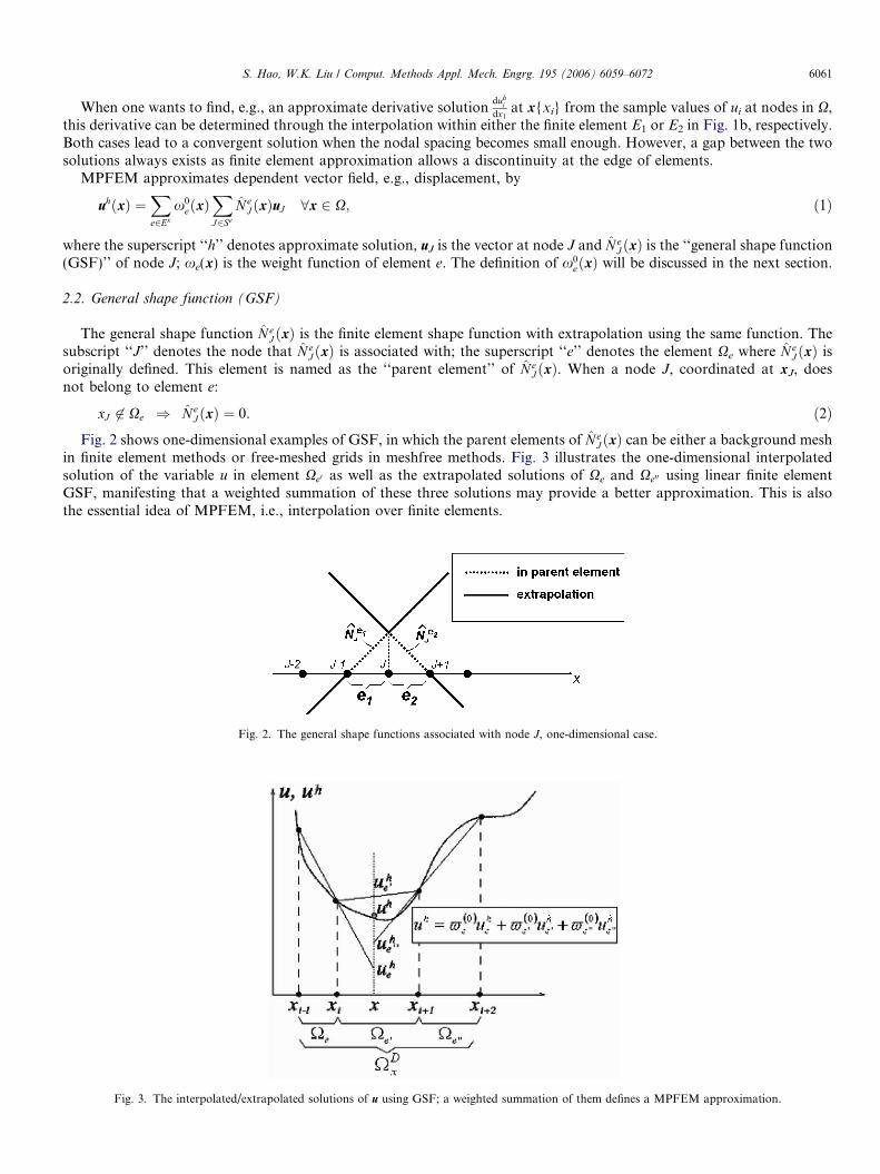
2.2. General shape function (GSF)

The general shape function N̂ eJðxÞ is the finite element shape function with extrapolation using the same function. The

subscript ‘‘J’’ denotes the node that N̂ eJðxÞ is associated with; the superscript ‘‘e’’ denotes the element Xe where N̂ e

J ðxÞ isoriginally defined. This element is named as the ‘‘parent element’’ of N̂ e

JðxÞ. When a node J, coordinated at xJ, doesnot belong to element e:

xJ 62 Xe ) N̂ eJ ðxÞ ¼ 0. ð2Þ

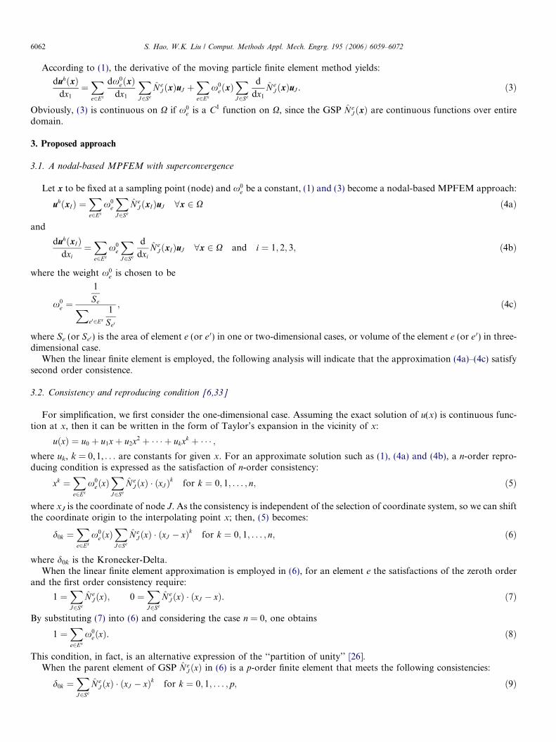
Fig. 2 shows one-dimensional examples of GSF, in which the parent elements of N̂ eJ ðxÞ can be either a background mesh

in finite element methods or free-meshed grids in meshfree methods. Fig. 3 illustrates the one-dimensional interpolatedsolution of the variable u in element Xe0 as well as the extrapolated solutions of Xe and Xe00 using linear finite elementGSF, manifesting that a weighted summation of these three solutions may provide a better approximation. This is alsothe essential idea of MPFEM, i.e., interpolation over finite elements.

Fig. 2. The general shape functions associated with node J, one-dimensional case.

Fig. 3. The interpolated/extrapolated solutions of u using GSF; a weighted summation of them defines a MPFEM approximation.


According to (1), the derivative of the moving particle finite element method yields:

duhðxÞdx1

¼Xe2Ex

dx0eðxÞ

dx1

XJ2Se

N̂ eJ ðxÞuJ þ

Xe2Ex

x0eðxÞ

XJ2Se

d

dx1

N̂ eJ ðxÞuJ . ð3Þ

Obviously, (3) is continuous on X if x0e is a C1 function on X, since the GSP N̂ e

J ðxÞ are continuous functions over entiredomain.

3. Proposed approach

3.1. A nodal-based MPFEM with superconvergence

Let x to be fixed at a sampling point (node) and x0e be a constant, (1) and (3) become a nodal-based MPFEM approach:

uhðxIÞ ¼Xe2Ex

x0e

XJ2Se

N̂ eJ ðxIÞuJ 8x 2 X ð4aÞ

and

duhðxIÞdxi

¼Xe2Ex

x0e

XJ2Se

d

dxiN̂ e

J ðxIÞuJ 8x 2 X and i ¼ 1; 2; 3; ð4bÞ

where the weight x0e is chosen to be

x0e ¼

1

SeXe02Ex

1

Se0

; ð4cÞ

where Se (or Se0) is the area of element e (or e 0) in one or two-dimensional cases, or volume of the element e (or e 0) in three-dimensional case.

When the linear finite element is employed, the following analysis will indicate that the approximation (4a)–(4c) satisfysecond order consistence.

3.2. Consistency and reproducing condition [6,33]

For simplification, we first consider the one-dimensional case. Assuming the exact solution of u(x) is continuous func-tion at x, then it can be written in the form of Taylor’s expansion in the vicinity of x:

uðxÞ ¼ u0 þ u1xþ u2x2 þ � � � þ ukxk þ � � � ;where uk, k = 0,1, . . . are constants for given x. For an approximate solution such as (1), (4a) and (4b), a n-order repro-ducing condition is expressed as the satisfaction of n-order consistency:

xk ¼Xe2Ex

x0eðxÞ

XJ2Se

N̂ eJ ðxÞ � ðxJ Þk for k ¼ 0; 1; . . . ; n; ð5Þ

where xJ is the coordinate of node J. As the consistency is independent of the selection of coordinate system, so we can shiftthe coordinate origin to the interpolating point x; then, (5) becomes:

d0k ¼Xe2Ex

x0eðxÞ

XJ2Se

N̂ eJ ðxÞ � ðxJ � xÞk for k ¼ 0; 1; . . . ; n; ð6Þ

where d0k is the Kronecker-Delta.When the linear finite element approximation is employed in (6), for an element e the satisfactions of the zeroth order

and the first order consistency require:

1 ¼XJ2Se

N̂ eJ ðxÞ; 0 ¼

XJ2Se

N̂ eJ ðxÞ � ðxJ � xÞ. ð7Þ

By substituting (7) into (6) and considering the case n = 0, one obtains

1 ¼Xe2Ex

x0eðxÞ. ð8Þ

This condition, in fact, is an alternative expression of the ‘‘partition of unity’’ [26].When the parent element of GSP N̂ e

J ðxÞ in (6) is a p-order finite element that meets the following consistencies:

d0k ¼XJ2Se

N̂ eJ ðxÞ � ðxJ � xÞk for k ¼ 0; 1; . . . ; p; ð9Þ


then, by substituting (9) into the reproducing condition (6) one can find that the latter has been satisfied for all n 6 p if (8)sustains.

In general, the kth order consistency for the mth order derivatives of MPFEM approximation (1) can be expressed as

m!dmk ¼Xe2Ex

dm

dxmx0

eðxÞXJ2Se

N̂ eJ ðxÞ

!� ðxJ � xÞk for k ¼ 0; 1; 2; . . . ; k P m. ð10Þ

For nodal-base MPFEM it can be proven that (10) can be satisfied for all k 6 p, m 6 k, where p is the order of the parentelement of the general shape function.

3.3. Determination of x0e

Considering the MPFEM as a particle method-based interpolation over finite element approximation, the weight x0e

represents the intersection between the domain of influence of a particle kernel /(x) and the domain of element e

[31,32]. Hence, the determination of x0e is in fact a process to design a kernel /(x) to obtain desirable convergence. Accord-

ing to (1), (4a) and (4b), the number of weight x0e in MPFEM approximation equals the number of elements confined by

Ex. When Ex contains only one element, the approximation (1) degenerates to conventional finite element and the weightx0

e is uniquely determined by (8), i.e., x0e � 1. However, when Ex contains k elements that k > 1, the partition of unity (8)

only defines a constraint of linear dependence for the set fx01;x

02; . . . ;x0

kg. In fact, after the satisfaction of (8), there are stillanother (k � 1) conditions which can be used to uniquely fix the values of all k components of x0

e . In the follows we intro-duce a scheme to determine x0

e by means of the satisfaction of higher order consistencies.In order to illustrate the concept, one-dimensional derivation will be conducted in follows. It will be trivial to extent the

results and conclusions into multi-dimensional cases.A simple choice is applying Shepher’s function:

x0e ¼

SeXe02Ex Se0

; e ¼ 1; 2; . . . ; k. ð11Þ

With this selection the convergence rate of the approximation (1), (3) and (4a), (4b) is essentially determined by the parentfinite element of general shape functions, even though the discontinuity on the finite element edge has been removed.

Not loss of generality, it is assumed that in (1–4) the parent element of general shape function is a p-order finite elementwith m nodes which sustains up to the pth order of consistencies:

xq ¼Xm

J¼1

N̂ eJ ðxÞ � ðxeJ Þq for q ¼ 1; 2; . . . ; p; ð12Þ

where ‘‘e’’ denotes the element e and xeJ is the coordinate of the Jth node in element e.Then the approximation (1) can be expressed as the following matrix form:

uhðxÞ ¼ N �U �W 0; ð13Þwhere

N ¼

N1 0

N2

� � �0 N k

26664

37775; U ¼

U1

U2

� � �Uk

26664

37775; W0 ¼

x01ðxÞ

x02ðxÞ� � �

x0kðxÞ

26664

37775 ð14Þ

and

N e ¼ N̂ e1ðxÞ � � � N̂ e

mðxÞ� �

; Ue ¼ ue1 � � � uem½ �T for e ¼ 1; 2; . . . ; k; ð15Þ

where ue1,ue2, . . . ,uem are the nodal displacements in element e. As an alternative expression of (5), the satisfaction of the(p + j)th consistencies can be written as

xpþj ¼ N � Xpþj �W 0; ð16Þ

where

Xpþj ¼ Xpþj1 � � � Xpþj

k

� �Tand Xpþj

e ¼ xpþje1 � � � xpþj

em

� �T; e ¼ 1; 2; . . . ; k. ð17Þ

By keeping (12) in mind, the weight x0eðxÞ that included by the vector W0 is solved through the satisfactions of (8) and the

(p + 1)th to (p + k � 1)th order of consistencies:


xpþj ¼ N � Xpþj �W 0 for j ¼ 1; 2; . . . ; k þ 1.

Hence,

W0 ¼ ðN � XÞ�1 � Rp; ð18Þwhere

X ¼ Xpþ1 Xpþ2 � � � Xpþk�1� �

; Rp ¼

1

xpþ1

� � �xpþk�1

26664

37775. ð19Þ

Since the interpolating point x is arbitrary, the procedure (12)–(19) is applicable for either nodal-based or Guassian qua-dratural-based MPFEM. Similarly, this scheme can also be applied for any particle method to determine the window (ker-nel) function by assigning p = 0 in (12)–(19).

3.4. Nodal integration

Due to the Kronecker-Delta of the general shape function, the approximation (4a) also possesses Kronecker-Deltaproperty when Ex is a compact domain that contains only the elements adjacent to node I while the partition of unity(8) has been satisfied:

uhðxIÞ ¼Xe2Ex

x0e

XJ2Se

N̂ eJ ðxIÞuJ ¼

Xe2Ex

x0eðdIJ uJ Þ ¼ ðdIJ uJ Þ

Xe2Ex

x0e ¼ uI ; ð20Þ

so the weight x0e is to be determined by the satisfaction of higher order consistence for derivative (4b). Similar to (13), the

matrix form of (4b) is

$uh ¼ $N �U �W 0; ð21Þwhere $ is the gradient operator: $f ¼ of

ox1; of

ox2; . . .

h i; in one-dimensional case: $f ¼ df

dx.

By repeating the procedure (13)–(19), one obtains

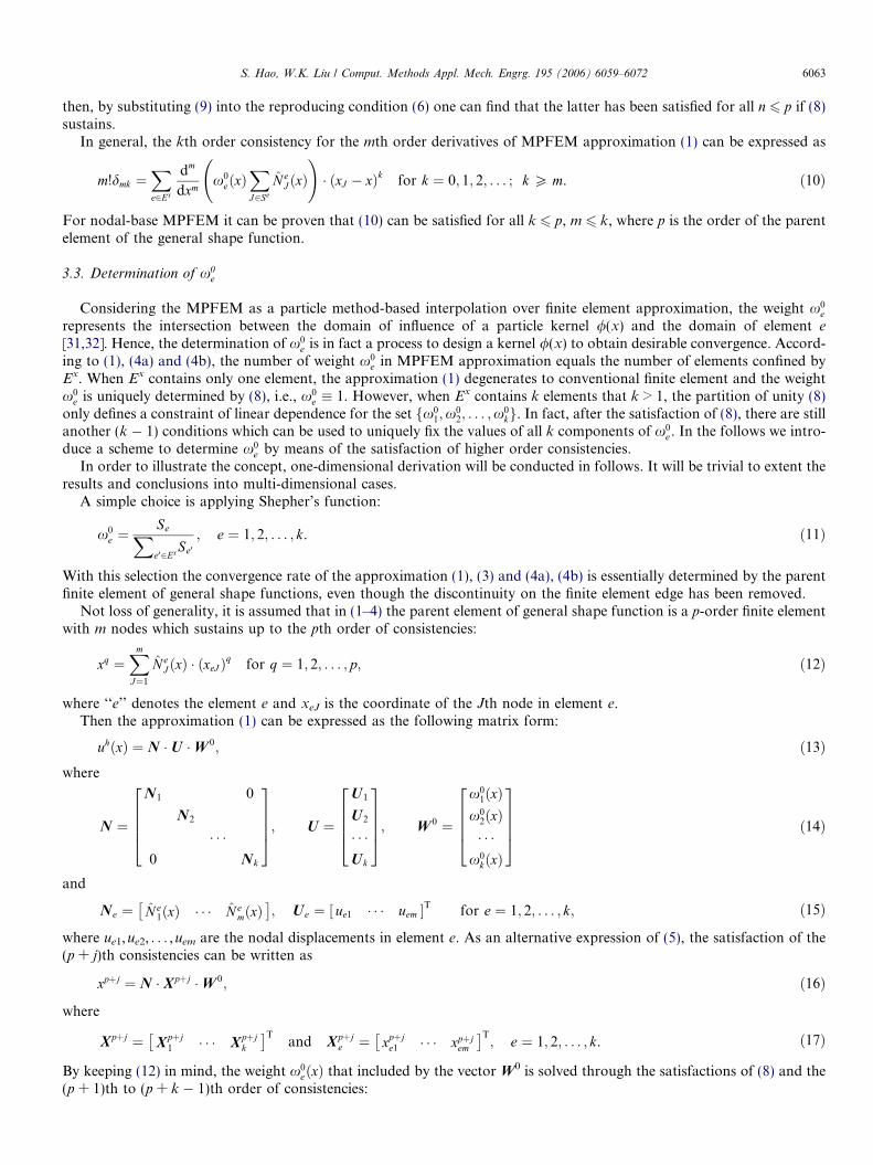
W0 ¼ ð$N � XÞ�1 � Rp. ð22ÞFor the one-dimensional example plotted in Fig. 4 with k = 2, p = 1, (4b), or (21), reads

duhðxÞdx

¼X2

i¼1

xð0ÞeiðxÞ �

X2

a¼1

dN̂ eia ðxÞ

dxua

( )¼

xð0Þe1ðxÞ

x2 � x1

½u2 � u1� þxð0Þe2ðxÞ

x3 � x2

½u3 � u2�. ð23Þ

Let x) x2 and u = x2, then (23) becomes

duhðx2Þdx

¼xð0Þe1

x2 � x1

½x22 � x2

1� þxð0Þe2

x3 � x2

½x23 � x2

2� ¼ 2x2fxð0Þe1þ xð0Þe2

g � ðx2 � x1Þxð0Þe1þ ðx3 � x2Þxð0Þe2

. ð24Þ

The solution of (21), i.e., the satisfactions of the partition of unity (8) and the second order consistence lead to

x2 � x1

x3 � x2

¼xð0Þe2

xð0Þe1

;

which is (4c).

3.5. Convergence at domain boundary

An obvious advantage of MPFEM is the satisfaction of Kronecker-Delta when a compact domain of influence isemployed. However, like the superconvergence in finite element, the above introduced scheme may not bring benefit when

Fig. 4. An one-dimensional example.


an interpolating point is located at boundary of the domain to be dealt with since the adjacent element number k in Ex maydegenerate to one. In the viewpoint of application, this drawback can be solved by implementing high order element atboundary to match the convergence inside the domain.

4. Numerical examples

4.1. 1-D numerical example

Consider the following one-dimensional boundary value problem (BVP) of function u:

o2uox2þ gðxÞ ¼ 0 8x 2 ½0; 1�; u;xn ¼ �t on Ct and u ¼ �u on Cu. ð25Þ

This example has been studied in [12]. Assuming that the ‘‘body force’’ g(x) in (25) has the form

gðxÞ ¼ 6xþ 2

a2� 2x� 2x0

a2

� �2 !

exp � x� x0

a

� �2� �

ð26Þ

and

uð0Þ ¼ exp � x20

a2

� �; ð27Þ

u;xð1Þ ¼ �3� 21� x0

a2

� �exp � 1� x0

a

� �2 !

; ð28Þ

where a is chosen to be small (e.g., a = 0.01) and x0 2 [0,1]. The solution to (25) is then

uðxÞ ¼ �x3 þ exp � x� x0

a

� �2� �

. ð29Þ

Numerical simulation using the proposed method has been conducted, in which the domain [0,1] has been partitioned intofinite element sub-domains separated by particles with spacing from 0.1 (11 particles) to 0.002 (500 particles). The L2 andH1 norms defined in [4] are computed:

ku� uhkL2¼

Z 1

0

ðu� uhÞ2 dx� 1=2

ð30Þ

and

ku� uhkH1¼

Z 1

0

ðu;x � uh;xÞ

2 dx� 1=2

. ð31Þ

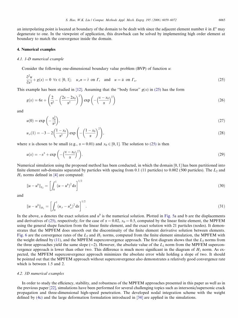
In the above, u denotes the exact solution and uh is the numerical solution. Plotted in Fig. 5a and b are the displacementsand derivatives of (25), respectively; for the case of a = 0.02, x0 = 0.5, computed by the linear finite element, the MPFEMusing the general shape function from the linear finite element, and the exact solution with 21 particles (nodes). It demon-strates that the MPFEM does smooth out the discontinuity of the finite element derivative solution between elements.Fig. 6 are the convergence rates of the L2 and H1 norms, computed from the finite element simulation, the MPFEM withthe weight defined by (11), and the MPFEM superconvergence approach. The first diagram shows that the L2 norms fromthe three approaches yield the same slope (=2). However, the absolute value of the L2 norm from the MPFEM supercon-vergence approach is lower than other two. This difference is much more significant in the diagram of H1 norm. As ex-pected, the MPFEM superconvergence approach minimizes the absolute error while holding a slope of two. It shouldbe pointed out that the MPFEM approach without superconvergence also demonstrates a relatively good convergence ratewhich is between 1.5 and 2.

4.2. 3D numerical examples

In order to study the efficiency, stability, and robustness of the MPFEM approaches presented in this paper as well as inthe previous paper [22], simulations have been performed for several challenging topics such as intersonic/supersonic crackpropagation and three-dimensional high-speed penetration. The developed nodal integration scheme with the weightdefined by (4c) and the large deformation formulation introduced in [34] are applied in the simulations.

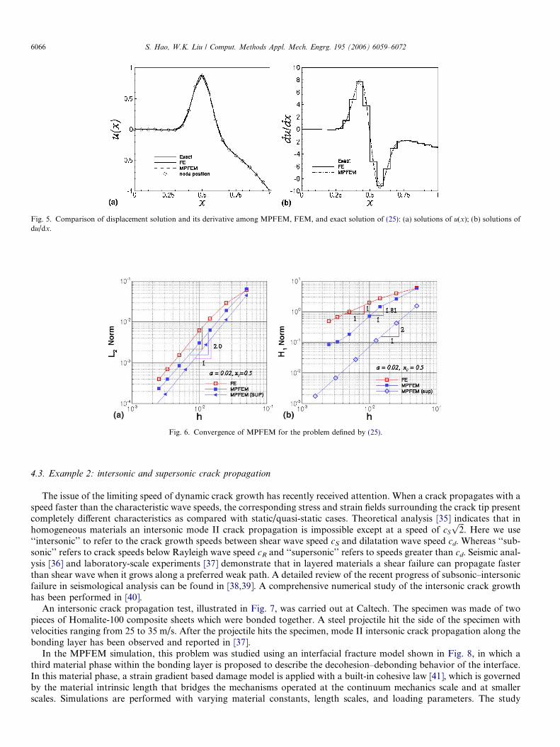
Fig. 5. Comparison of displacement solution and its derivative among MPFEM, FEM, and exact solution of (25): (a) solutions of u(x); (b) solutions ofdu/dx.

Fig. 6. Convergence of MPFEM for the problem defined by (25).


4.3. Example 2: intersonic and supersonic crack propagation

The issue of the limiting speed of dynamic crack growth has recently received attention. When a crack propagates with aspeed faster than the characteristic wave speeds, the corresponding stress and strain fields surrounding the crack tip presentcompletely different characteristics as compared with static/quasi-static cases. Theoretical analysis [35] indicates that inhomogeneous materials an intersonic mode II crack propagation is impossible except at a speed of cS

ffiffiffi2p

. Here we use‘‘intersonic’’ to refer to the crack growth speeds between shear wave speed cS and dilatation wave speed cd. Whereas ‘‘sub-sonic’’ refers to crack speeds below Rayleigh wave speed cR and ‘‘supersonic’’ refers to speeds greater than cd. Seismic anal-ysis [36] and laboratory-scale experiments [37] demonstrate that in layered materials a shear failure can propagate fasterthan shear wave when it grows along a preferred weak path. A detailed review of the recent progress of subsonic–intersonicfailure in seismological analysis can be found in [38,39]. A comprehensive numerical study of the intersonic crack growthhas been performed in [40].

An intersonic crack propagation test, illustrated in Fig. 7, was carried out at Caltech. The specimen was made of twopieces of Homalite-100 composite sheets which were bonded together. A steel projectile hit the side of the specimen withvelocities ranging from 25 to 35 m/s. After the projectile hits the specimen, mode II intersonic crack propagation along thebonding layer has been observed and reported in [37].

In the MPFEM simulation, this problem was studied using an interfacial fracture model shown in Fig. 8, in which athird material phase within the bonding layer is proposed to describe the decohesion–debonding behavior of the interface.In this material phase, a strain gradient based damage model is applied with a built-in cohesive law [41], which is governedby the material intrinsic length that bridges the mechanisms operated at the continuum mechanics scale and at smallerscales. Simulations are performed with varying material constants, length scales, and loading parameters. The study

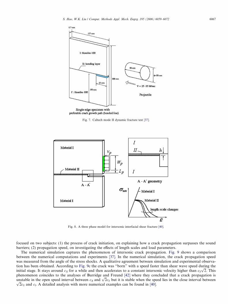
Fig. 7. Caltech mode II dynamic fracture test [37].

Fig. 8. A three phase model for intersonic interfacial shear fracture [40].


focused on two subjects: (1) the process of crack initiation, on explaining how a crack propagation surpasses the soundbarriers; (2) propagation speed, on investigating the effects of length scales and load parameters.

The numerical simulation captures the phenomenon of intersonic crack propagation. Fig. 9 shows a comparisonbetween the numerical computations and experiments [37]. In the numerical simulation, the crack propagation speedwas measured from the angle of the stress shocks. A qualitative agreement between simulation and experimental observa-tion has been obtained. According to Fig. 9c the crack was ‘‘born’’ with a speed faster than shear wave speed during theinitial stage. It stays around cS for a while and then accelerates to a constant intersonic velocity higher than cS

ffiffiffi2p

. Thisphenomenon coincides to the analyses of Burridge and Freund [42] where they concluded that a crack propagation isunstable in the open speed interval between cS and

ffiffiffi2p

cS but it is stable when the speed lies in the close interval betweenffiffiffi2p

cS and cl. A detailed analysis with more numerical examples can be found in [40].

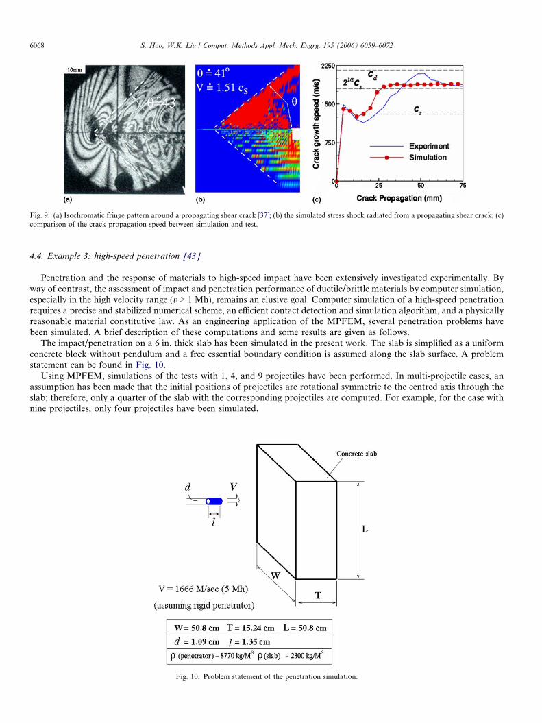
Fig. 9. (a) Isochromatic fringe pattern around a propagating shear crack [37]; (b) the simulated stress shock radiated from a propagating shear crack; (c)comparison of the crack propagation speed between simulation and test.


4.4. Example 3: high-speed penetration [43]

Penetration and the response of materials to high-speed impact have been extensively investigated experimentally. Byway of contrast, the assessment of impact and penetration performance of ductile/brittle materials by computer simulation,especially in the high velocity range (v > 1 Mh), remains an elusive goal. Computer simulation of a high-speed penetrationrequires a precise and stabilized numerical scheme, an efficient contact detection and simulation algorithm, and a physicallyreasonable material constitutive law. As an engineering application of the MPFEM, several penetration problems havebeen simulated. A brief description of these computations and some results are given as follows.

The impact/penetration on a 6 in. thick slab has been simulated in the present work. The slab is simplified as a uniformconcrete block without pendulum and a free essential boundary condition is assumed along the slab surface. A problemstatement can be found in Fig. 10.

Using MPFEM, simulations of the tests with 1, 4, and 9 projectiles have been performed. In multi-projectile cases, anassumption has been made that the initial positions of projectiles are rotational symmetric to the centred axis through theslab; therefore, only a quarter of the slab with the corresponding projectiles are computed. For example, for the case withnine projectiles, only four projectiles have been simulated.

Fig. 10. Problem statement of the penetration simulation.


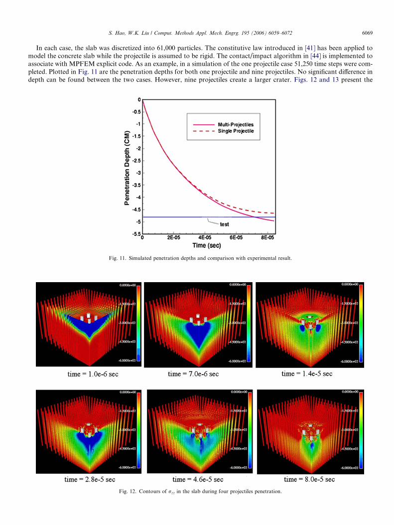
In each case, the slab was discretized into 61,000 particles. The constitutive law introduced in [41] has been applied tomodel the concrete slab while the projectile is assumed to be rigid. The contact/impact algorithm in [44] is implemented toassociate with MPFEM explicit code. As an example, in a simulation of the one projectile case 51,250 time steps were com-pleted. Plotted in Fig. 11 are the penetration depths for both one projectile and nine projectiles. No significant difference indepth can be found between the two cases. However, nine projectiles create a larger crater. Figs. 12 and 13 present the

Fig. 11. Simulated penetration depths and comparison with experimental result.

Fig. 12. Contours of rzz in the slab during four projectiles penetration.

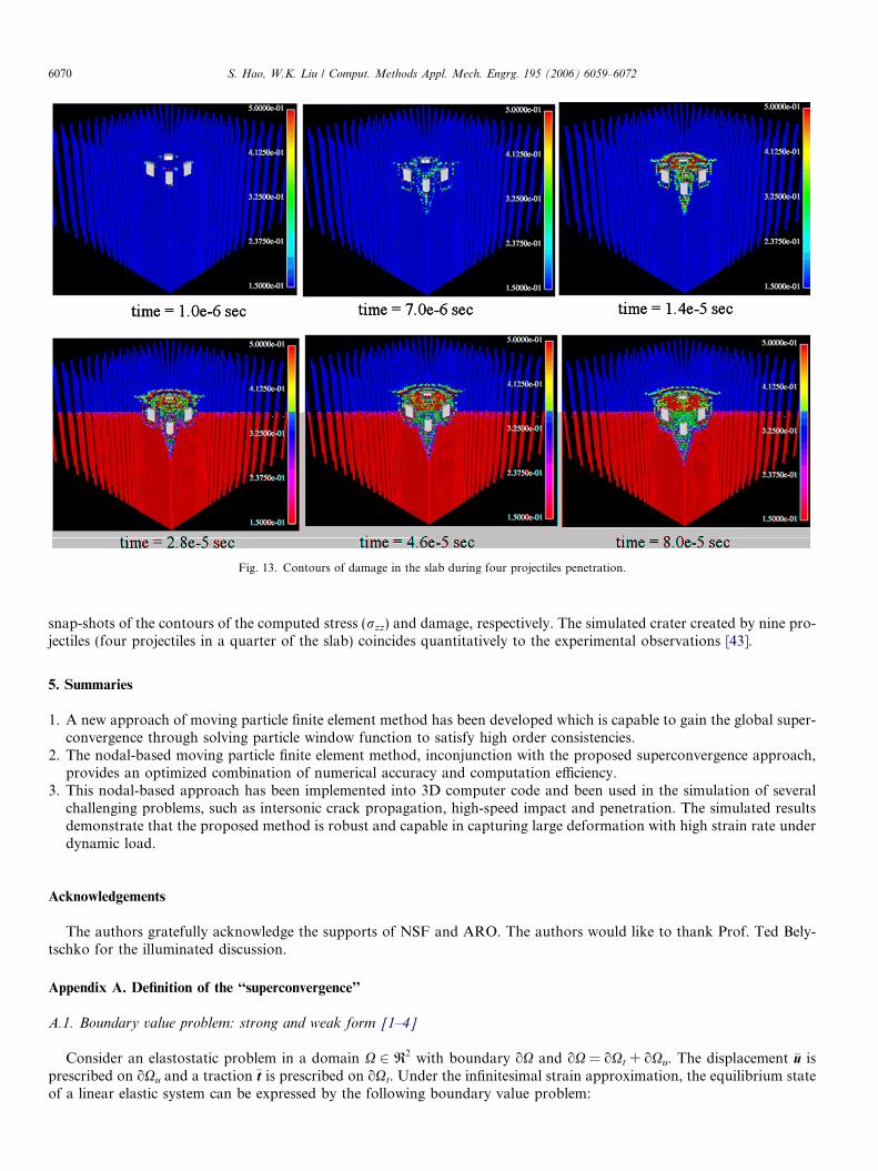
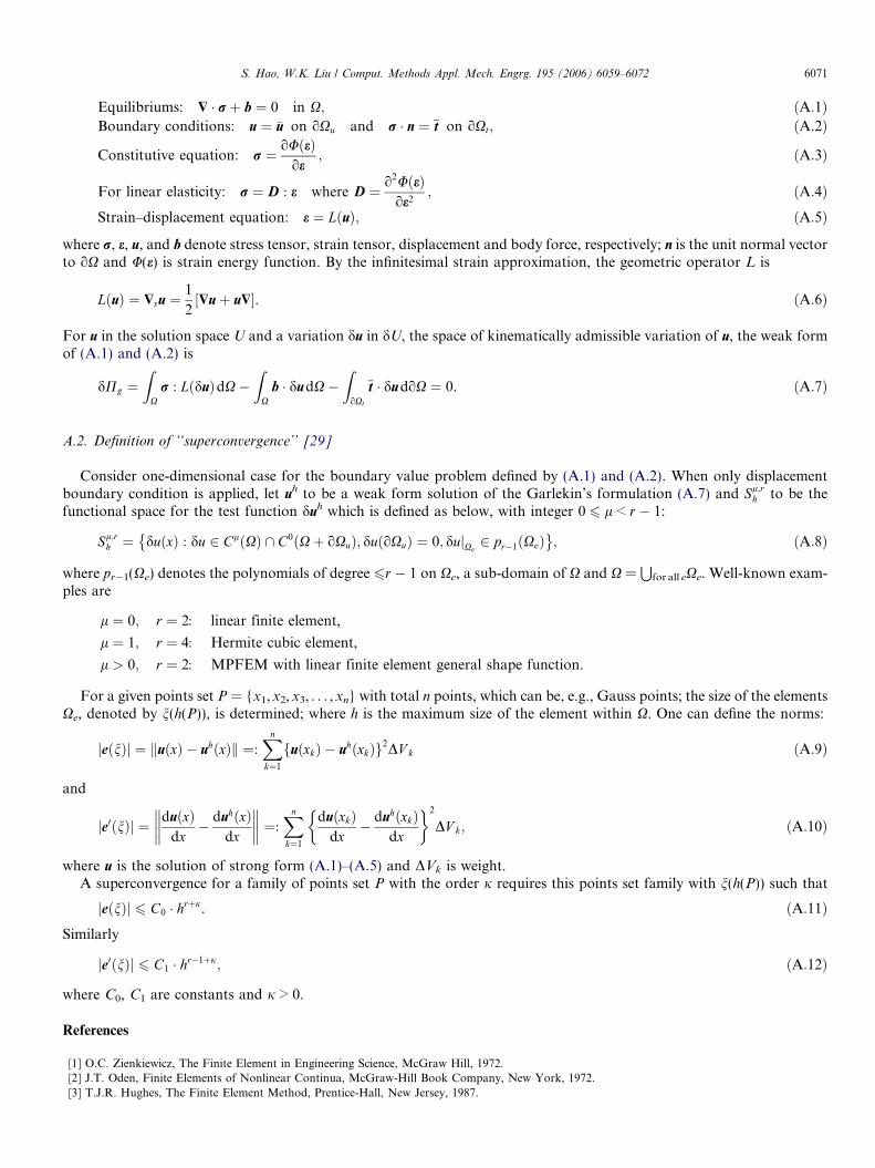
Fig. 13. Contours of damage in the slab during four projectiles penetration.


snap-shots of the contours of the computed stress (rzz) and damage, respectively. The simulated crater created by nine pro-jectiles (four projectiles in a quarter of the slab) coincides quantitatively to the experimental observations [43].

5. Summaries

1. A new approach of moving particle finite element method has been developed which is capable to gain the global super-convergence through solving particle window function to satisfy high order consistencies.

2. The nodal-based moving particle finite element method, inconjunction with the proposed superconvergence approach,provides an optimized combination of numerical accuracy and computation efficiency.

3. This nodal-based approach has been implemented into 3D computer code and been used in the simulation of severalchallenging problems, such as intersonic crack propagation, high-speed impact and penetration. The simulated resultsdemonstrate that the proposed method is robust and capable in capturing large deformation with high strain rate underdynamic load.

Acknowledgements

The authors gratefully acknowledge the supports of NSF and ARO. The authors would like to thank Prof. Ted Bely-tschko for the illuminated discussion.

Appendix A. Definition of the ‘‘superconvergence’’

A.1. Boundary value problem: strong and weak form [1–4]

Consider an elastostatic problem in a domain X 2 R2 with boundary oX and oX = oXt + oXu. The displacement �u isprescribed on oXu and a traction �t is prescribed on oXt. Under the infinitesimal strain approximation, the equilibrium stateof a linear elastic system can be expressed by the following boundary value problem:


Equilibriums: $ � rþ b ¼ 0 in X; ðA:1ÞBoundary conditions: u ¼ �u on oXu and r � n ¼ �t on oXt; ðA:2Þ

Constitutive equation: r ¼ oUðeÞoe

; ðA:3Þ

For linear elasticity: r ¼ D : e where D ¼ o2UðeÞoe2

; ðA:4ÞStrain–displacement equation: e ¼ LðuÞ; ðA:5Þ

where r, e, u, and b denote stress tensor, strain tensor, displacement and body force, respectively; n is the unit normal vectorto oX and U(e) is strain energy function. By the infinitesimal strain approximation, the geometric operator L is

LðuÞ ¼ $su ¼1

2½$uþ u$�. ðA:6Þ

For u in the solution space U and a variation du in dU, the space of kinematically admissible variation of u, the weak formof (A.1) and (A.2) is

dPg ¼Z

Xr : LðduÞdX�

ZX

b � dudX�Z

oXt

�t � dudoX ¼ 0. ðA:7Þ

A.2. Definition of ‘‘superconvergence’’ [29]

Consider one-dimensional case for the boundary value problem defined by (A.1) and (A.2). When only displacementboundary condition is applied, let uh to be a weak form solution of the Garlekin’s formulation (A.7) and Sl;r

h to be thefunctional space for the test function duh which is defined as below, with integer 0 6 l < r � 1:

Sl;rh ¼ duðxÞ : du 2 ClðXÞ \ C0ðXþ oXuÞ; duðoXuÞ ¼ 0; dujXe

2 pr�1ðXeÞ� �

; ðA:8Þ

where pr�1(Xe) denotes the polynomials of degree 6r � 1 on Xe, a sub-domain of X and X =S

for all eXe. Well-known exam-ples are

l ¼ 0; r ¼ 2: linear finite element,

l ¼ 1; r ¼ 4: Hermite cubic element,

l > 0; r ¼ 2: MPFEM with linear finite element general shape function.

For a given points set P = {x1,x2,x3, . . . ,xn} with total n points, which can be, e.g., Gauss points; the size of the elementsXe, denoted by n(h(P)), is determined; where h is the maximum size of the element within X. One can define the norms:

jeðnÞj ¼ kuðxÞ � uhðxÞk ¼:Xn

k¼1

fuðxkÞ � uhðxkÞg2DV k ðA:9Þ

and

je0ðnÞj ¼ duðxÞdx� duhðxÞ

dx

¼:

Xn

k¼1

duðxkÞdx

� duhðxkÞdx

� �2

DV k; ðA:10Þ

where u is the solution of strong form (A.1)–(A.5) and DVk is weight.A superconvergence for a family of points set P with the order j requires this points set family with n(h(P)) such that

jeðnÞj 6 C0 � hrþj. ðA:11ÞSimilarly

je0ðnÞj 6 C1 � hr�1þj; ðA:12Þ

where C0, C1 are constants and j > 0.

References

[1] O.C. Zienkiewicz, The Finite Element in Engineering Science, McGraw Hill, 1972.[2] J.T. Oden, Finite Elements of Nonlinear Continua, McGraw-Hill Book Company, New York, 1972.[3] T.J.R. Hughes, The Finite Element Method, Prentice-Hall, New Jersey, 1987.


[4] T. Belytschko, W.K. Liu, B. Moran, Nonlinear Finite Elements for Continua and Structures, John Wiley & Sons, New York, 2000.[5] T. Belytschko, Y.Y. Lu, L. Gu, Element-free Galerkin methods, Int. J. Numer. Methods Engrg. 37 (1994) 229–256.[6] W.K. Liu, S. Jun, Y.F. Zhang, Reproducing kernel particle methods, Int. J. Numer. Methods Fluids 20 (1995) 1081–1106.[7] J.T. Oden, C.A.M. Duarte, O.C. Zienkiewicz, A new cloud-based hp finite element method, Comput. Methods Appl. Mech. Engrg. 153 (1998) 117–

126.[8] C.A. Duarte, J.T. Oden, An h–p adaptive method using clouds, Comput. Methods Appl. Mech. Engrg. 139 (1–4) (1996) 237–262.[9] P. Randles, L. Libersky, Smoothed particle hydrodynamics: some recent improvements and applications, Comput. Methods Appl. Mech. Engrg. 139

(1996) 375–408.[10] G.J. Wagner, W.K. Liu, Application of essential boundary conditions in mesh-free methods: a corrected collocation method, Int. J. Numer. Methods

Engrg. 47 (2000) 1367–1379.[11] J. Bonet, S. Kulasegaram, Correction and stabilization of smooth particle hydrodynamics methods with applications in metal forming simulations,

Int. J. Numer. Methods Engrg. 47 (2000) 1189–1214.[12] J. Dolbow, T. Belytschko, Numerical integration of the Galerkin weak form in meshfree methods, Comput. Mech. 23 (3) (1999) 219–230.[13] I. Babuska, U. Banerjee, J.E. Osborn, Survey of meshless and generalized finite element methods: a unified approach, Acta Numer. 12 (2003) 1–125.[14] S.F. Li, W.K. Liu, Meshfree and particle methods and their applications, Appl. Mech. Rev. 55 (2002) 1–34.[15] S.F. Li, K. Wing, Meshfree Particle Methods, Springer, 2004.[16] T. Belytschko, T. Black, Elastic crack growth in finite elements with minimal remeshing, Int. J. Numer. Methods Engrg. 45 (5) (1999) 601–620.[17] B. Nayroles, G. Touzot, P. Villon, The diffuse elements method, Comptes Rendus De L Academie Des Sciences Serie Ii 313 (2) (1991) 133–138.[18] N. Sukumar, B. Moran, T. Belytschko, The natural element method in solid mechanics, Int. J. Numer. Methods Engrg. 43 (5) (1998) 839.[19] T. Strouboulis, I. Babuska, K. Copps, The design and analysis of the generalized finite element method, Int. J. Numer. Methods Engrg. 181 (2000)

43–69.[20] A. Huerta, S. Fernandez-Mendez, Enrichment and coupling of the finite element and meshless methods, Int. J. Numer. Methods Engrg. 48 (11) (2000)

1615–1636.[21] J.S. Chen, S.P. Yoon, C.T. Wu, Non-linear version of stabilized conforming nodal integration for Galerkin mesh-free methods, Int. J. Numer.

Methods Engrg. 53 (12) (2002) 2587–2615.[22] S. Hao, W.K. Liu, C.T. Chang, Computer implementation of damage models by finite element and meshfree methods, Comput. Methods Appl.

Mech. Engrg. 187 (2000) 401–440.[23] S.R. De, K.E. Bathe, The method of finite spheres with improved numerical integration, Comput. Struct. 79 (22–25) (2001) 2183–2196.[24] S.N. Atluri, T.L. Zhu, New concepts in meshless methods, Int. J. Numer. Methods Engrg. 47 (1–3) (2000) 537–556.[25] W.K. Liu, S.F. Li, T. Belytschko, Moving least-square reproducing kernel methods. 1. Methodology and convergence, Comput. Methods Appl.

Mech. Engrg. 143 (1–2) (1997) 113–154.[26] I. Babuska, J.M. Melenk, The partition of unity method, Int. J. Numer. Methods Engrg. 40 (1997) 727–758.[27] G. Yagawa, Node-by-node parallel finite elements: a virtually meshless method, Int. J. Numer. Methods Engrg. 60 (1) (2004) 69–102.[28] I. Babuska et al., Computer-based proof of the existence of superconvergence points in the finite element method; superconvergence of the derivative

in finite element solutions of Laplace’s, Poission’s, and the elasticity equations, Numer. Methods Partial Differen. Equat. 12 (1996) 347–392.[29] L.B. Wahlbin, Superconvergence in Galerkin finite element methods, in: F.T. Groningen (Ed.), Lecture Notes in Mathematics, vol. 1605, Springer,

1995.[30] S. Hao, H.S. Park, W.K. Liu, Moving particle finite element method, Int. J. Numer. Methods Engrg. 53 (8) (2002) 1937–1958.[31] S. Hao, Liu, W.K. Revisit of moving particle finite element method, in: Fifth World Congress on Computational Mechanics, Vienna, Austria, 2002.

On-line publication (ISBN 3-9501554-0-6).[32] S. Hao, W.K. Liu, T. Belytschko, Moving particle finite element method with global smoothness, Int. J. Numer. Methods Engrg. 59 (2004) 1007–

1020.[33] T. Belytschko, Y. Krongauz, J. Dolbow, C. Gerlach, On the completeness of meshfree particle methods, Int. J. Numer. Methods Engrg. 43 (5) (1998)

785–812.[34] T.J.R. Hughes, J. Winget, Finite rotation effects in numerical integration of rate constitutive equations arising in large-deformation analysis, Int. J.

Numer. Methods Engrg. 15 (1980) 1862–1867.[35] L.B. Freund, Mechanics of dynamic shear crack-propagation, J. Geophys. Res. 84 (NB5) (1979) 2199–2209.[36] M. Bouchon et al., How fast is rupture during an earthquake? New insights from the 1999 Turkey earthquakes, Geophys. Res. Lett. 28 (14) (2001)

2723–2726.[37] A.J. Rosakis, O. Samudrala, D. Coker, Cracks faster than the shear wave speed, Science 284 (5418) (1999) 1337–1340.[38] R. Dmowska, J.R. Rice, Fracture theory and its seismological application, in: E.R. Teisseyre (Ed.), Continuum Theories in Solid Earth Physics,

Elsevier, 1986.[39] A.J. Rosakis, Intersonic shear cracks and fault ruptures, 2001.[40] S. Hao, W.K. Liu, A. Rosakis, P. Klein, Modeling and simulation of intersonic crack growth, Northwestern University, M. Engineering, 2001.[41] S. Hao, W.K. Liu, P. Klein, Multi-Scale Damage Model, Chicago, IL, USA, IUTAM2000, 2000.[42] C.R.G. Burridge, L.B. Freund, Stability of a rapid mode-II shear crack with finite cohesive traction, J. Geophys. Res. 84 (NB5) (1979) 2210–2222.[43] S. Hao et al., DTRW Reports II, 2000.[44] T. Belytschko, M.O. Neal, Contact-impact by the pinball algorithm with penalty and Lagrangian-methods, Int. J. Numer. Methods Engrg. 31 (3)

(1991) 547–572.

Documents

Moving particle ﬁnite element method with superconvergence · Moving particle ﬁnite element method with superconvergence: Nodal integration formulation and applications q Su Hao