Moving interface problems

for elliptic systems

John Strain

Mathematics Department

UC Berkeley

June 2010

1

ALGORITHMS

Implicit semi-Lagrangian contouring moves interfaces

– with arbitrary topology

– subject to stiff interface velocity

using

∗ implicit interface representation

∗ implicit stiffly-stable time discretization

Locally-corrected spectral methods find velocity from

– overdetermined first-order elliptic systems in bulk phases

– geometric boundary conditions on moving interfaces

using

∗ boundary integral equations

∗ generalized Ewald summation

∗ local correction formulas

∗ geometric nonuniform fast Fourier transforms

2

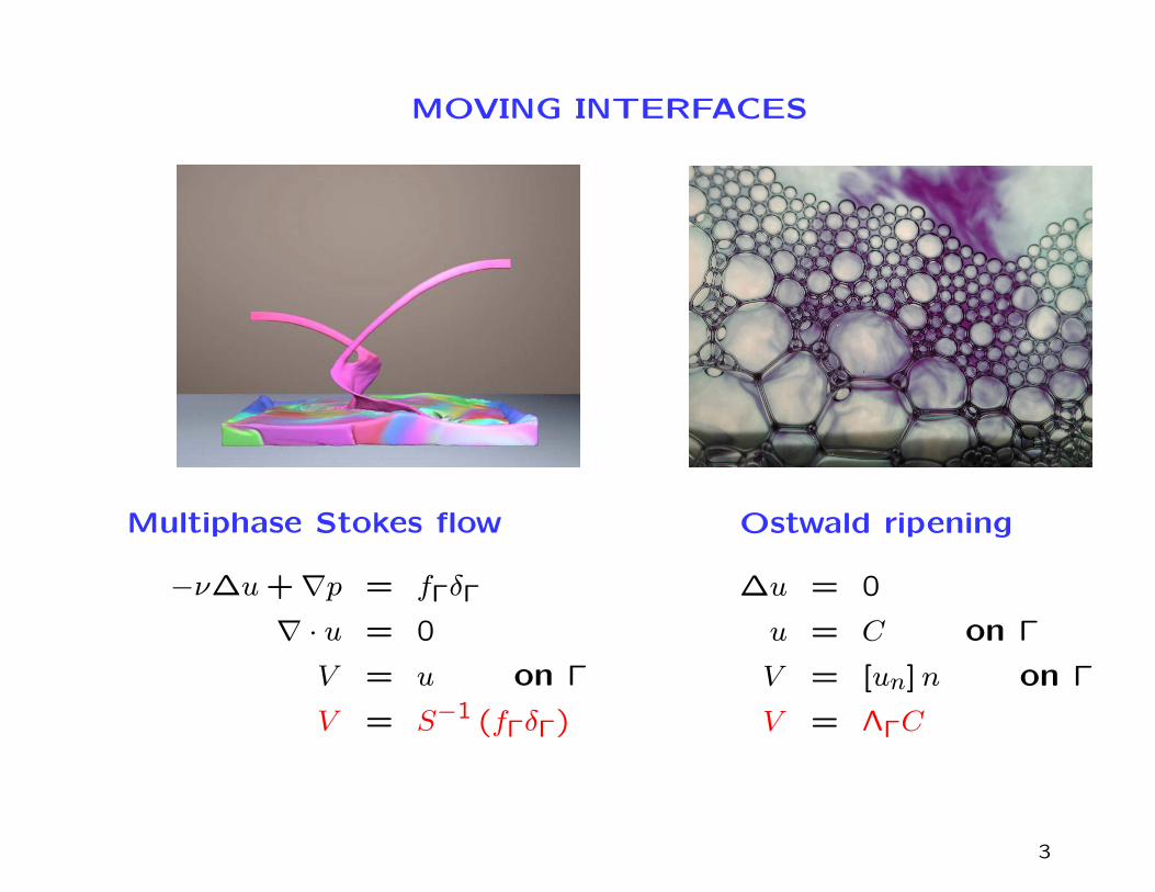
MOVING INTERFACES

Multiphase Stokes flow

−ν∆u+∇p = fΓδΓ

∇ · u = 0

V = u on Γ

V = S−1 (fΓδΓ)

Ostwald ripening

∆u = 0

u = C on Γ

V = [un]n on Γ

V = ΛΓC

3

STIFF INTERFACES

Normal velocity V on Γ(t) depends on

– material properties, experimental parameters, . . .

– interface geometry, topology, dynamics, . . .

Sensitive dependence produces stiff interfaces

Curvature flow

V = C

k = O(h2)

Ostwald ripening

V = ΛΓC

k = O(h3)

Surface diffusion

V = ∆ΓC

k = O(h4)

Computationally expensive dilemma

– explicit methods require tiny time steps

– implicit methods must solve nonlinear systems

4

IMPLICIT CONTOURING APPROACH

Represent interface Γ(t) implicitly as

zero set of signed distance function

d(x) = ± minγ∈Γ(t)

‖x− γ‖

Extend V (γ, t) to fictitious global velocity field W (x, t)

and transport values of d globally with velocity W

Contour: New interface Γ(t+ k) is zero set x|ϕ(x) = 0 of

ϕ(x) = d(x)

where x = c(t) is foot of backward characteristic

c(s) = W (c(s), s) entering x = c(t+ k) at time s = t+ k

5

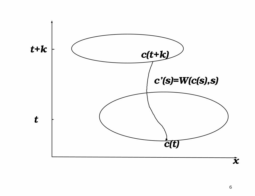
c(t+k)

c(t)

x

c’(s)=W(c(s),s)

t+k

t

6

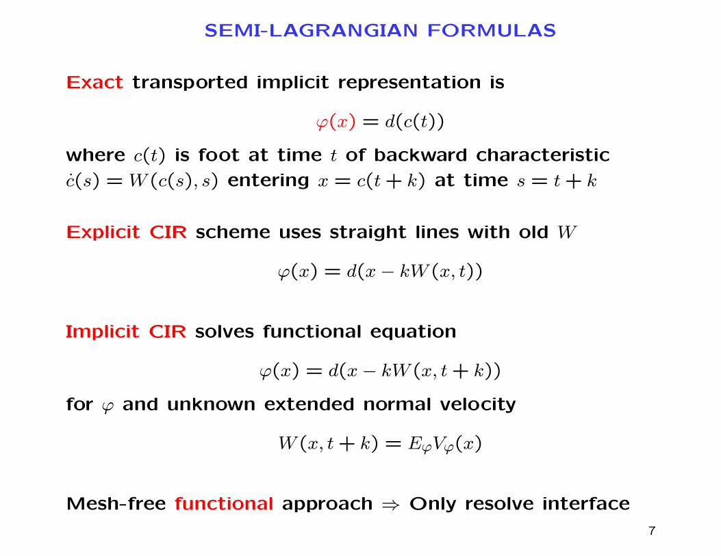
SEMI-LAGRANGIAN FORMULAS

Exact transported implicit representation is

ϕ(x) = d(c(t))

where c(t) is foot at time t of backward characteristic

c(s) = W (c(s), s) entering x = c(t+ k) at time s = t+ k

Explicit CIR scheme uses straight lines with old W

ϕ(x) = d(x− kW (x, t))

Implicit CIR solves functional equation

ϕ(x) = d(x− kW (x, t+ k))

for ϕ and unknown extended normal velocity

W (x, t+ k) = EϕVϕ(x)

Mesh-free functional approach ⇒ Only resolve interface

7

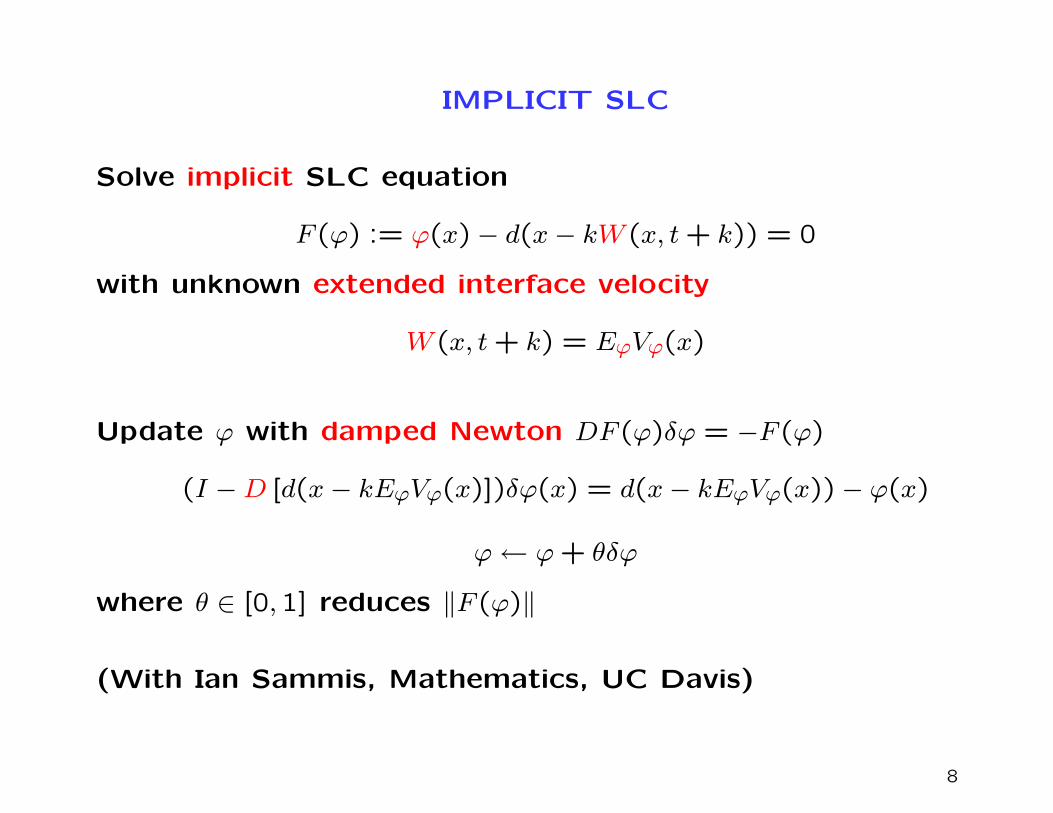
IMPLICIT SLC

Solve implicit SLC equation

F (ϕ) := ϕ(x)− d(x− kW (x, t+ k)) = 0

with unknown extended interface velocity

W (x, t+ k) = EϕVϕ(x)

Update ϕ with damped Newton DF (ϕ)δϕ = −F (ϕ)

(I −D [d(x− kEϕVϕ(x)])δϕ(x) = d(x− kEϕVϕ(x))− ϕ(x)

ϕ← ϕ+ θδϕ

where θ ∈ [0,1] reduces ‖F (ϕ)‖

(With Ian Sammis, Mathematics, UC Davis)

8

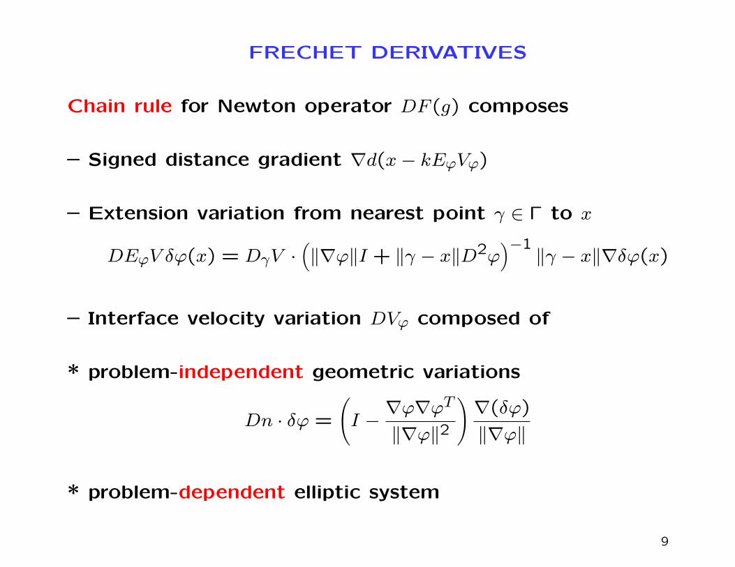
FRECHET DERIVATIVES

Chain rule for Newton operator DF (g) composes

– Signed distance gradient ∇d(x− kEϕVϕ)

– Extension variation from nearest point γ ∈ Γ to x

DEϕV δϕ(x) = DγV ·(‖∇ϕ‖I + ‖γ − x‖D2ϕ

)−1‖γ − x‖∇δϕ(x)

– Interface velocity variation DVϕ composed of

* problem-independent geometric variations

Dn · δϕ =

(I −∇ϕ∇ϕT

‖∇ϕ‖2

)∇(δϕ)

‖∇ϕ‖

* problem-dependent elliptic system

9

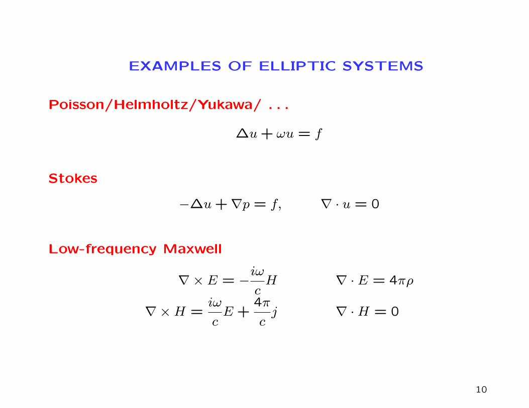
EXAMPLES OF ELLIPTIC SYSTEMS

Poisson/Helmholtz/Yukawa/ . . .

∆u+ ωu = f

Stokes

−∆u+∇p = f, ∇ · u = 0

Low-frequency Maxwell

∇× E = −iω

cH ∇ · E = 4πρ

∇×H =iω

cE +

4π

cj ∇ ·H = 0

10

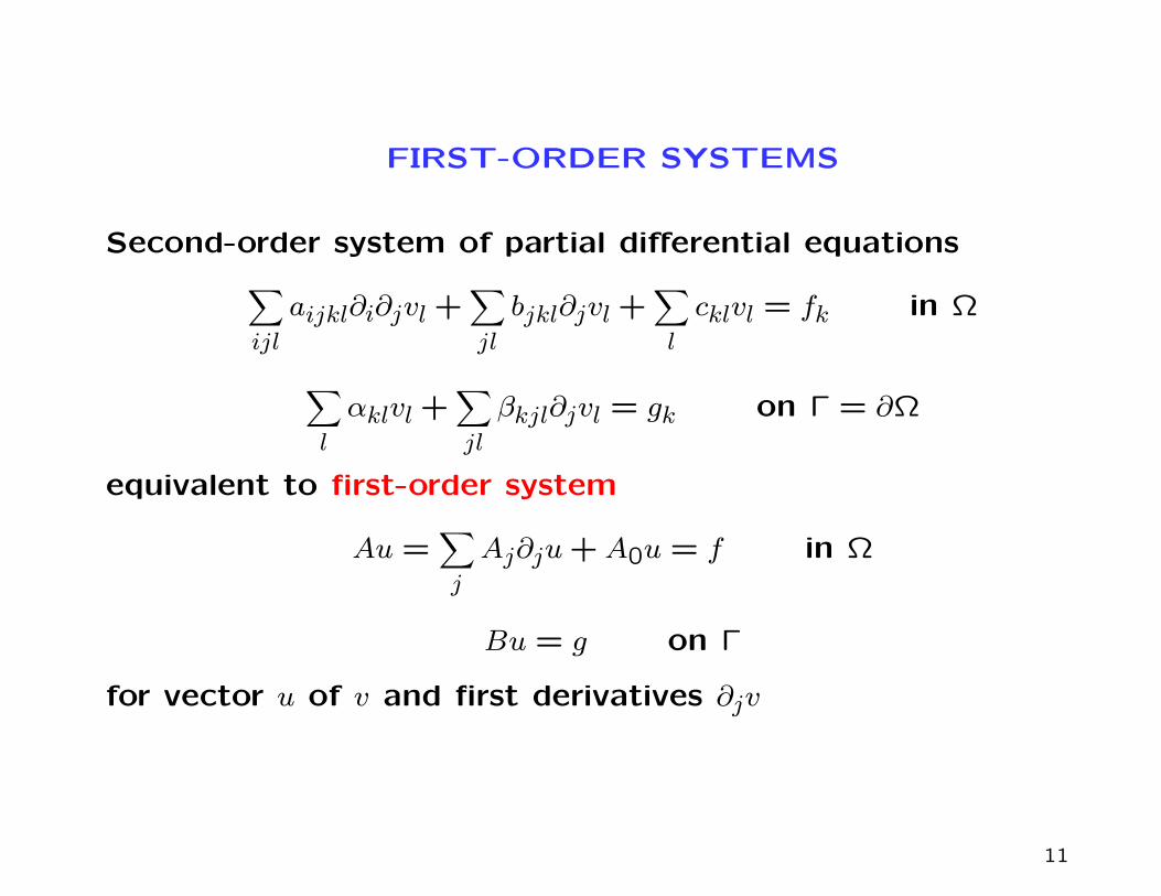
FIRST-ORDER SYSTEMS

Second-order system of partial differential equations∑ijl

aijkl∂i∂jvl +∑jl

bjkl∂jvl +∑l

cklvl = fk in Ω

∑l

αklvl +∑jl

βkjl∂jvl = gk on Γ = ∂Ω

equivalent to first-order system

Au =∑j

Aj∂ju+A0u = f in Ω

Bu = g on Γ

for vector u of v and first derivatives ∂jv

11

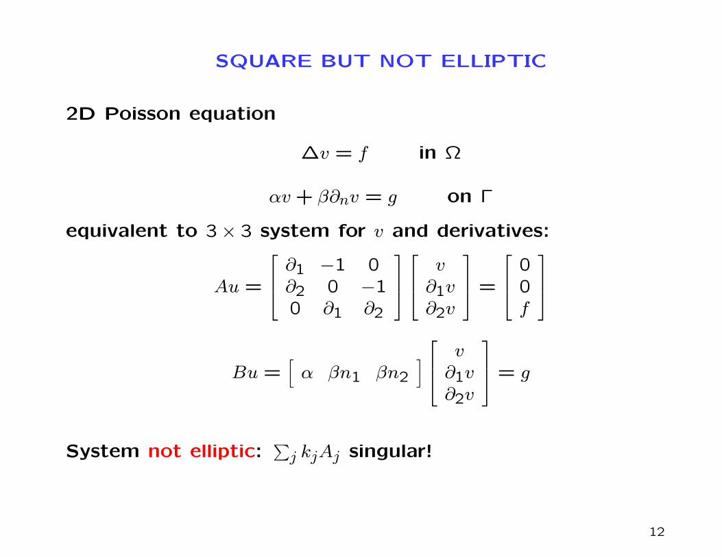
SQUARE BUT NOT ELLIPTIC

2D Poisson equation

∆v = f in Ω

αv + β∂nv = g on Γ

equivalent to 3× 3 system for v and derivatives:

Au =

∂1 −1 0∂2 0 −10 ∂1 ∂2

v∂1v∂2v

=

00f

Bu =[α βn1 βn2

] v∂1v∂2v

= g

System not elliptic:∑j kjAj singular!

12

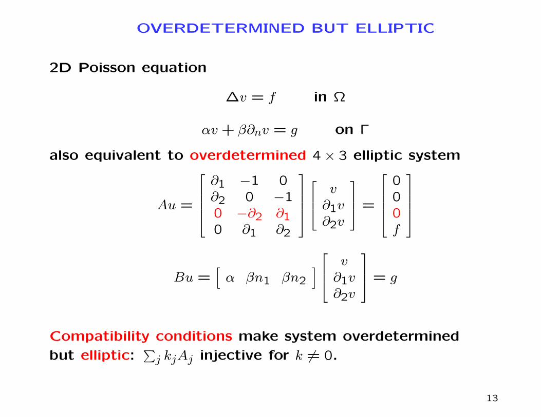
OVERDETERMINED BUT ELLIPTIC

2D Poisson equation

∆v = f in Ω

αv + β∂nv = g on Γ

also equivalent to overdetermined 4× 3 elliptic system

Au =

∂1 −1 0∂2 0 −10 −∂2 ∂10 ∂1 ∂2

v∂1v∂2v

=

000f

Bu =[α βn1 βn2

] v∂1v∂2v

= g

Compatibility conditions make system overdetermined

but elliptic:∑j kjAj injective for k 6= 0.

13

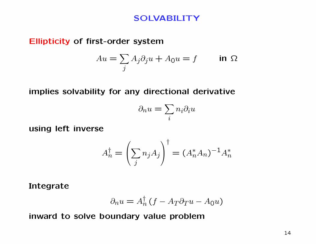
SOLVABILITY

Ellipticity of first-order system

Au =∑j

Aj∂ju+A0u = f in Ω

implies solvability for any directional derivative

∂nu =∑i

ni∂iu

using left inverse

A†n =

∑j

njAj

† = (A∗nAn)−1A∗n

Integrate

∂nu = A†n (f −AT∂Tu−A0u)

inward to solve boundary value problem

14

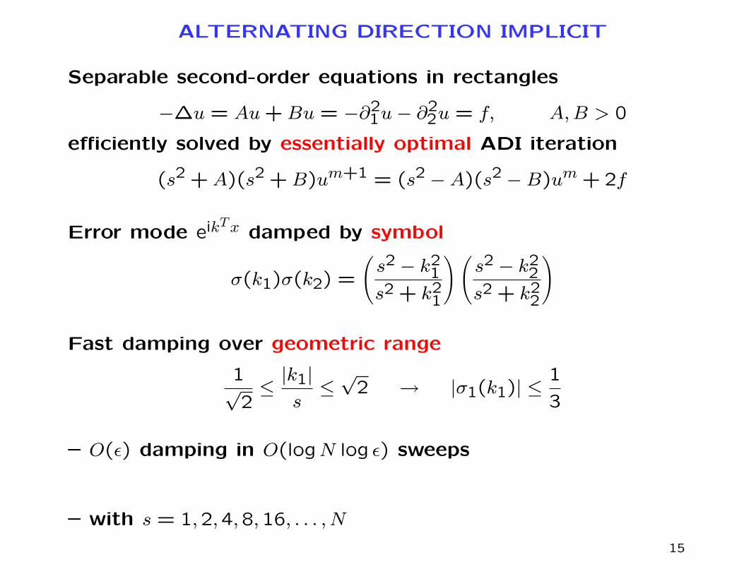
ALTERNATING DIRECTION IMPLICIT

Separable second-order equations in rectangles

−∆u = Au+Bu = −∂21u− ∂

22u = f, A,B > 0

efficiently solved by essentially optimal ADI iteration

(s2 +A)(s2 +B)um+1 = (s2 −A)(s2 −B)um + 2f

Error mode eikTx damped by symbol

σ(k1)σ(k2) =

(s2 − k2

1

s2 + k21

)(s2 − k2

2

s2 + k22

)

Fast damping over geometric range

1√2≤|k1|s≤√

2 → |σ1(k1)| ≤1

3

– O(ε) damping in O(logN log ε) sweeps

– with s = 1,2,4,8,16, . . . , N

15

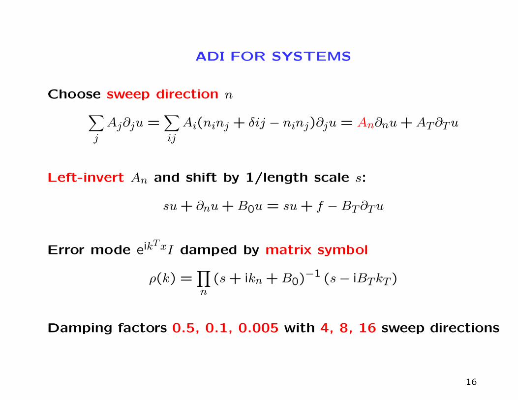
ADI FOR SYSTEMS

Choose sweep direction n∑j

Aj∂ju =∑ij

Ai(ninj + δij − ninj)∂ju = An∂nu+AT∂Tu

Left-invert An and shift by 1/length scale s:

su+ ∂nu+B0u = su+ f −BT∂Tu

Error mode eikTxI damped by matrix symbol

ρ(k) =∏n

(s+ ikn +B0)−1 (s− iBTkT )

Damping factors 0.5, 0.1, 0.005 with 4, 8, 16 sweep directions

16

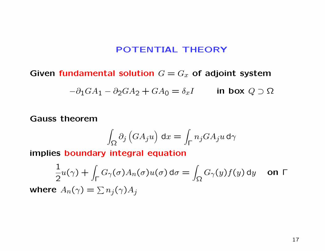
POTENTIAL THEORY

Given fundamental solution G = Gx of adjoint system

−∂1GA1 − ∂2GA2 +GA0 = δxI in box Q ⊃ Ω

Gauss theorem ∫Ω∂j(GAju

)dx =

∫ΓnjGAjudγ

implies boundary integral equation

1

2u(γ) +

∫ΓGγ(σ)An(σ)u(σ) dσ =

∫ΩGγ(y)f(y) dy on Γ

where An(γ) =∑nj(γ)Aj

17

PROJECTED INTEGRAL EQUATION

Project out boundary condition Bu = g with P (γ) = I −B∗B

Solve well-conditioned square system

1

2µ(γ) +

∫ΓP (γ)Gγ(σ)An(σ)µ(σ)dσ = ρ(γ)

for projected unknown µ = Pu with data

ρ(γ) = P (γ)∫

ΩGγ(y)f(y) dy + P (γ)

∫ΓGγ(σ)An(σ)B∗g(σ) dσ

Recover u = µ+B∗g on Γ and

u(x) =∫

ΩGx(y)f(y) dy +

∫ΓGx(σ)An(σ)u(σ) dσ in Ω

Need fast algorithm for Gγ(σ)

18

FUNDAMENTAL SOLUTION IN A BOX

Fourier series in box enclosing Γ gives fundamental solution

Gx(y) =∑k∈Zd

e−ikTxs(k)−1a∗(k)eikTy

where s = a∗a is positive definite Hermitian matrix and

a(k) = id∑

j=1

kjAj +A0

Filter with e−τs for exponentially fast convergence:

Gx(y) =∑‖k‖≤N

e−ikTxe−τs(k)s(k)−1a∗(k)eikTy

up to O(e−τN2) truncation error and O(τ) local error

19

GENERALIZED EWALD SUMMATION

Fundamental solution is smooth rapidly-converging series

Gτ(x) =∑

e−τs(k)s(k)−1a∗(k)e−ikTx

plus local asymptotic error expansion

Eτ = (I − e−τS)S−1A∗ =

(τ −

τ2

2!S +

τ3

3!S2 − · · ·

)A∗

with local differential operators A∗ and S = A∗A

Implies many local correction methods

for Laplace, Helmholtz, Stokes, . . .

Also effective for volume and layer potentials

20

HIGHER-ORDER GAUSS THEOREM

Gauss theorem differentiates indicator function ω(x) of set Ω:∫Ω∂judx =

∫Γnjudγ ⇔ ∂jω = njδΓ

Geometry in second-order derivatives

∂j∂kω(x) = (∂jnk)δΓ + njnk∂nδΓ

Volume potential of discontinuous function fω splits:∫ΩGx(y)f(y) dy = B(fω) = BF (fω) +BL(fω)

Local correction BL satisfies product rule:

BL(fω)(x) = τ

(A∗f(x))ω(x)−∑j

A∗jf(x)nj(x)δΓ(x)

+O(τ2)

21

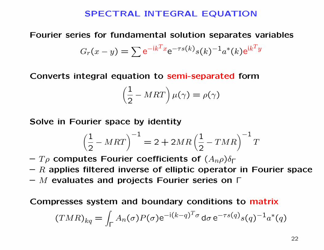
SPECTRAL INTEGRAL EQUATION

Fourier series for fundamental solution separates variables

Gr(x− y) =∑

e−ikTxe−τs(k)s(k)−1a∗(k)eikTy

Converts integral equation to semi-separated form(1

2−MRT

)µ(γ) = ρ(γ)

Solve in Fourier space by identity(1

2−MRT

)−1= 2 + 2MR

(1

2− TMR

)−1T

– Tρ computes Fourier coefficients of (Anρ)δΓ– R applies filtered inverse of elliptic operator in Fourier space

– M evaluates and projects Fourier series on Γ

Compresses system and boundary conditions to matrix

(TMR)kq =∫

ΓAn(σ)P (σ)e−i(k−q)Tσ dσ e−τs(q)s(q)−1a∗(q)

22

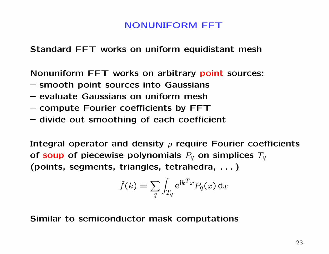
NONUNIFORM FFT

Standard FFT works on uniform equidistant mesh

Nonuniform FFT works on arbitrary point sources:

– smooth point sources into Gaussians

– evaluate Gaussians on uniform mesh

– compute Fourier coefficients by FFT

– divide out smoothing of each coefficient

Integral operator and density ρ require Fourier coefficients

of soup of piecewise polynomials Pq on simplices Tq

(points, segments, triangles, tetrahedra, . . . )

f(k) =∑q

∫Tq

eikTxPq(x) dx

Similar to semiconductor mask computations

23

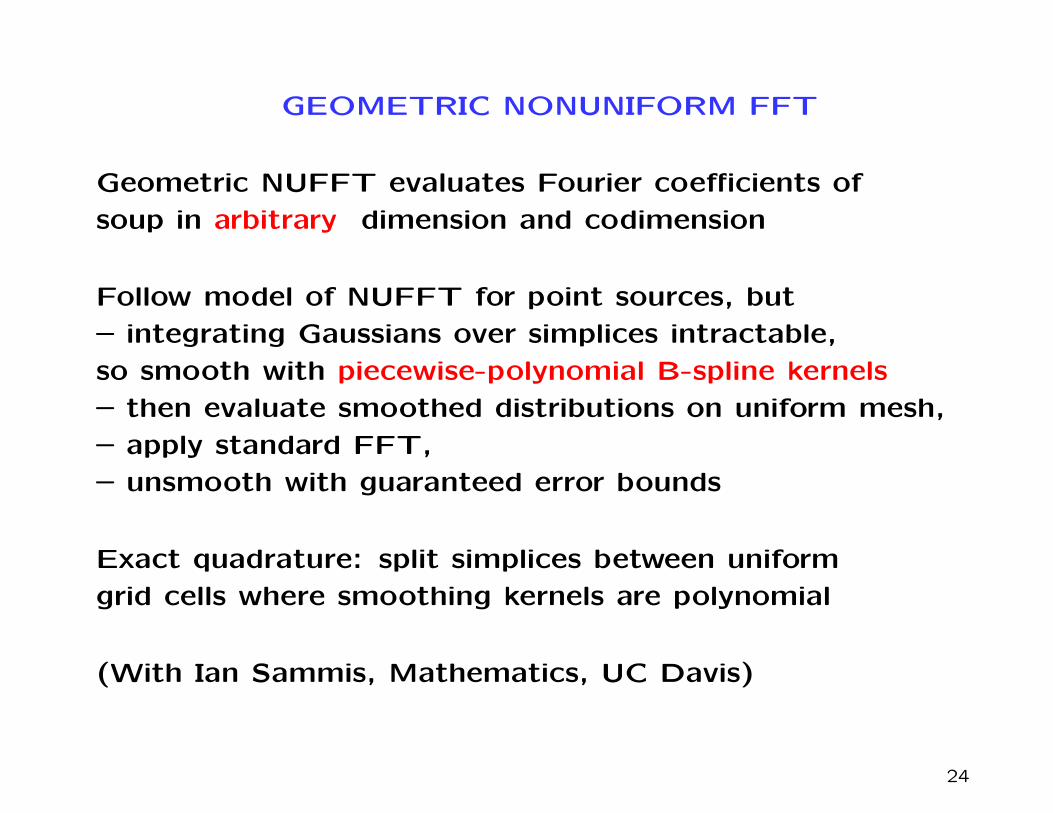
GEOMETRIC NONUNIFORM FFT

Geometric NUFFT evaluates Fourier coefficients of

soup in arbitrary dimension and codimension

Follow model of NUFFT for point sources, but

– integrating Gaussians over simplices intractable,

so smooth with piecewise-polynomial B-spline kernels

– then evaluate smoothed distributions on uniform mesh,

– apply standard FFT,

– unsmooth with guaranteed error bounds

Exact quadrature: split simplices between uniform

grid cells where smoothing kernels are polynomial

(With Ian Sammis, Mathematics, UC Davis)

24

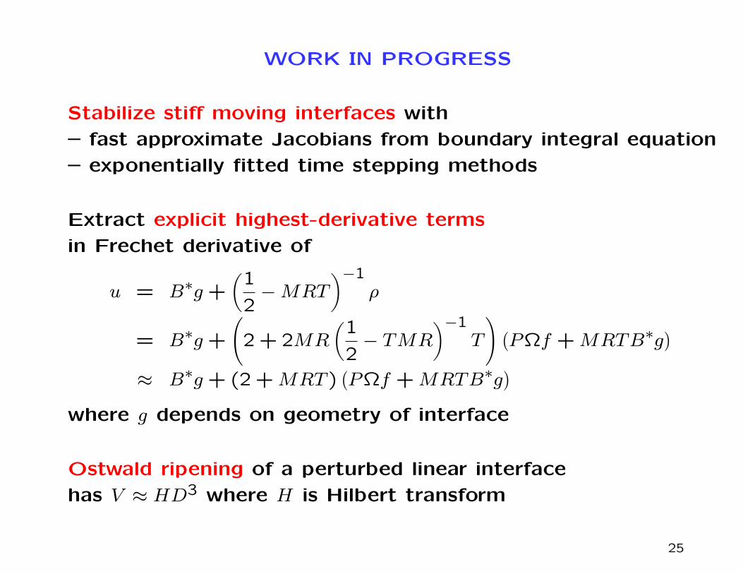
WORK IN PROGRESS

Stabilize stiff moving interfaces with

– fast approximate Jacobians from boundary integral equation

– exponentially fitted time stepping methods

Extract explicit highest-derivative terms

in Frechet derivative of

u = B∗g +(

1

2−MRT

)−1ρ

= B∗g +

(2 + 2MR

(1

2− TMR

)−1T

) (PΩf +MRTB∗g

)≈ B∗g + (2 +MRT )

(PΩf +MRTB∗g

)where g depends on geometry of interface

Ostwald ripening of a perturbed linear interface

has V ≈ HD3 where H is Hilbert transform

25