Mound Study Project Cape Fear, North Carolina Pre …cfried/reports/2003/Battisto_Friedrichs_2003_EHI... · Mound Study Project Cape Fear, North Carolina Pre-Deployment Calibration

Mound Study Project

Cape Fear, North Carolina Pre-Deployment Calibration

Of OBS and ADV Sensors June/July 2001

EHI Project No. 6000.21

February 2003 Final VIMS Report CHSD-2003-05 Prepared for Evans-Hamilton, Inc

By

Grace M. Battisto and Carl T. Friedrichs Phone: 804-884-7606, -7303; Fax: 804-684-7198

Email: [email protected]; [email protected]

Department of Physical Sciences Virginia Institute of Marine Science

Gloucester Point, VA 23062

Battisto and Friedrichs, Mound Study Project, Sensor Calibrations i

TABLE OF CONTENTS Page TABLE OF CONTENTS i

LIST OF TABLES ii

LIST OF FIGURES iii

1. SUMMARY 1

2. METHODS 2

2.1 Sediment Collection 2

2.2 OBS Calibration 3

2.3 ADV Calibration 6

3. RESULTS

3.1 OBS Calibration 6

3.2 ADV Calibration 7

Battisto and Friedrichs, Mound Study Project, Sensor Calibrations ii

LIST OF TABLES

Table Page

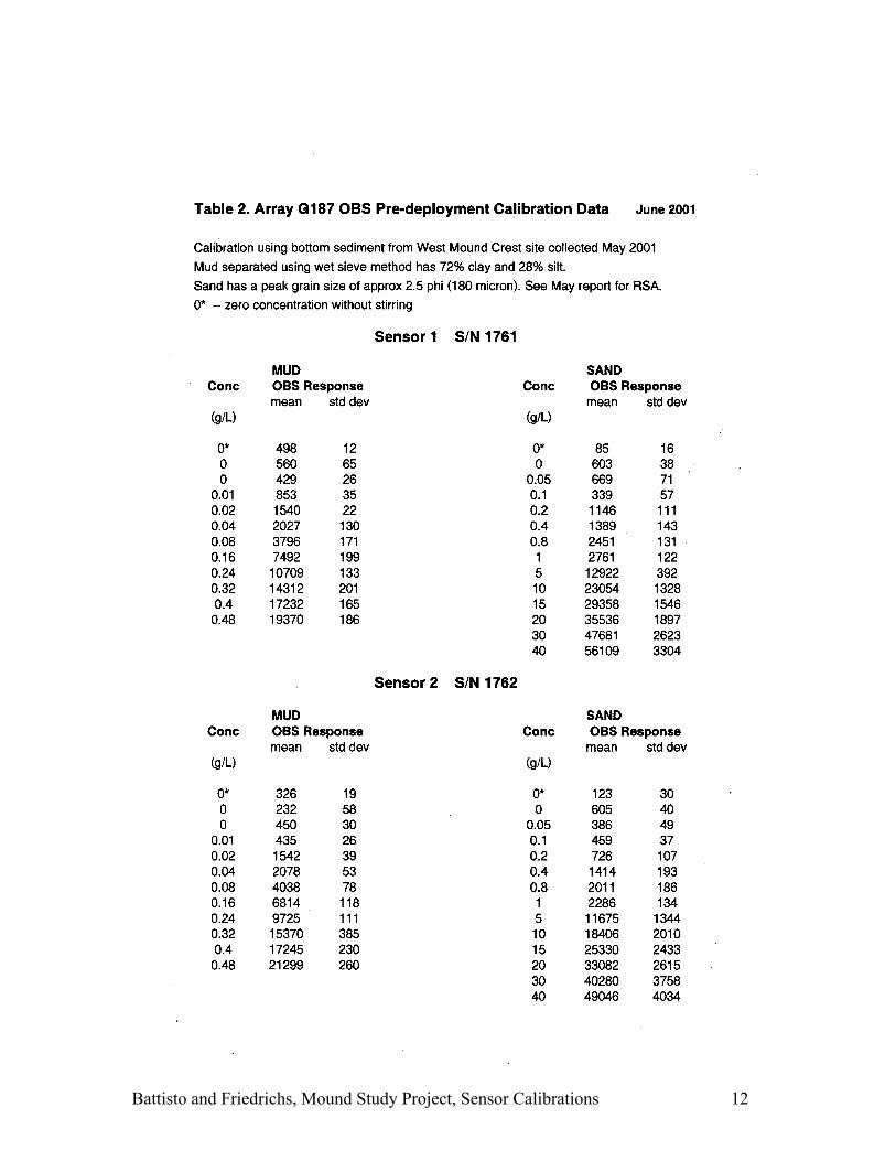
1 Array G181 OBS Pre-deployment calibration data 8

2 Array G187 OBS Pre-deployment calibration data 12

3 Array G181 ADV B205 Pre-deployment calibration data 16

4 Array G187 ADV B211 Pre-deployment calibration data 16

5 Summary of Best-Fit Coefficients and estimates of their errors for all OBS and ADV sensors 18

Battisto and Friedrichs, Mound Study Project, Sensor Calibrations iii

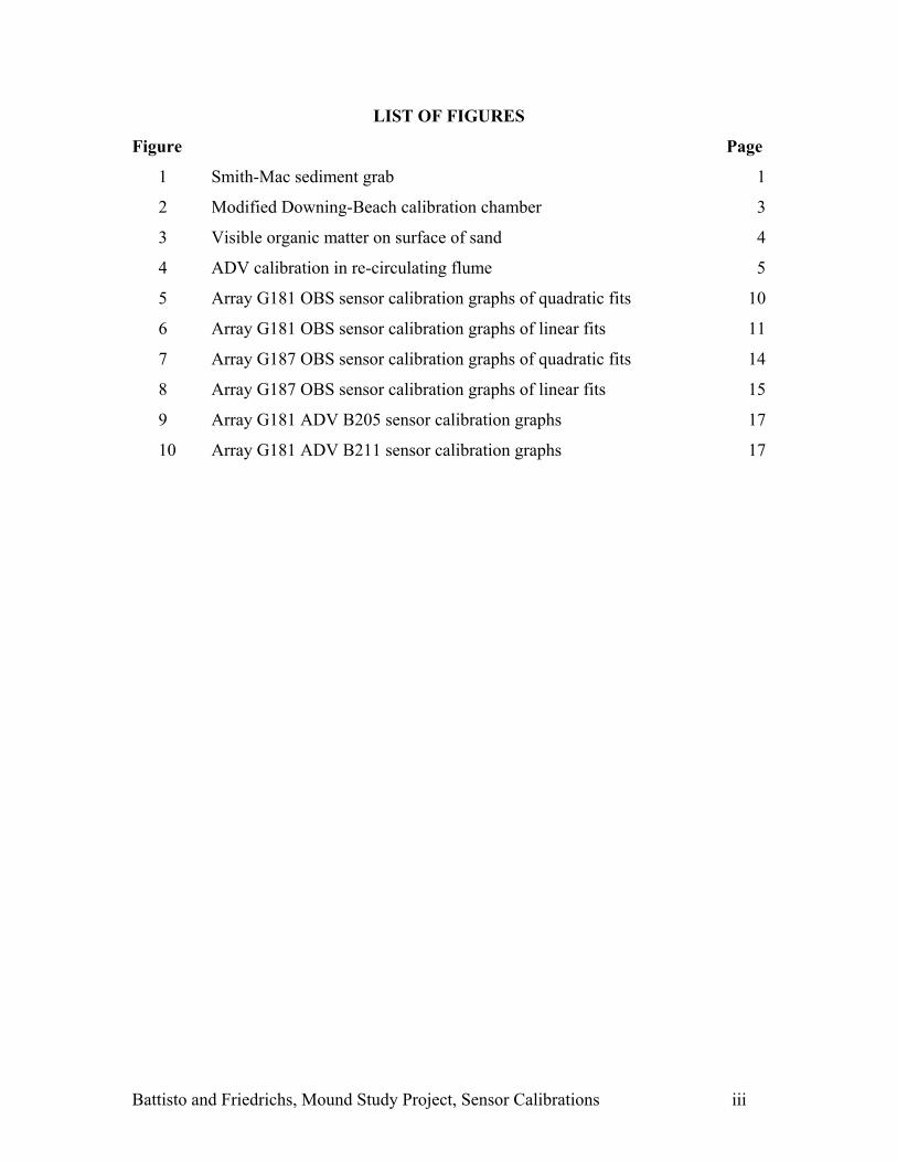
LIST OF FIGURES

Figure Page

1 Smith-Mac sediment grab 1

2 Modified Downing-Beach calibration chamber 3

3 Visible organic matter on surface of sand 4

4 ADV calibration in re-circulating flume 5

5 Array G181 OBS sensor calibration graphs of quadratic fits 10

6 Array G181 OBS sensor calibration graphs of linear fits 11

7 Array G187 OBS sensor calibration graphs of quadratic fits 14

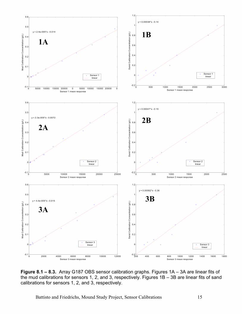
8 Array G187 OBS sensor calibration graphs of linear fits 15

9 Array G181 ADV B205 sensor calibration graphs 17

10 Array G181 ADV B211 sensor calibration graphs 17

Battisto and Friedrichs, Mound Study Project, Sensor Calibrations 1

1. SUMMARY

This work was conducted in support of an ongoing investigation of sediment dispersal

and evolution of a mixed-sediment disposal mound off Cape Fear, NC, by the US Army

Corps of Engineers (USACE) and Evans-Hamilton, Inc. (EHI), project number 6000.21.

Two Sontek Acoustic Doppler Velocimeter (ADV) arrays equipped with three D&A

Optical Backscatter Sensors each were calibrated at the Virginia Institute of Marine

Science in specialized calibration chambers to verify the instruments’ response range to

water velocity (ADVs) or suspended sediment concentration (OBSs) before deployment.

Calibrations showed stable OBS response to suspended sediment with linear curves at

low concentrations and quadratic curves at high concentrations. ADV response to current

speed was stable and linear with gains and offsets consistent with the factory calibration.

Figure 1. Smith-Mac bottom sediment grab used to collect the top approximately 10 cm with the sediment-water interface left relatively intact.


2. METHOD

The Sontek array case G187 was equipped with ADV B211 and OBS sensors 1 through 3

(S/N 1761, 1762 and 1763 respectively). Array case G181 was equipped with ADV B205

Sensors and OBS sensors 1 through 3 (S/N 1764, 1768 and 1769). June 2001 calibrations

were attempted for all sensors. Array G187 calibrations were successful. Array G181 had

connector problems and was sent back to Evans-Hamilton, Inc., after failed attempts to

communicate with the ADV and OBS sensors. The connector was repaired and the unit

returned to VIMS. The second attempt to calibrate Array G181 in July was successful.

Sontek “Sonterm” software was used to communicate with the instruments. The June

calibrations were hurried due to delay in shipment of the instrument Arrays to VIMS and

the tight deadline for deployment of the instruments. Thus in June there was not enough

time to become familiar with the Sonterm software. Therefore 10 records were recorded

by hand and averaged for each OBS sensor at each concentration, and 7 records were

recorded and averaged for each water velocity used to calibrate the ADV sensors. In July,

familiarization with the Sonterm software allowed log files of over 100 records each to be

collected and averaged for each calibration point in the second attempt to calibrate the

G181 sensor.

2.1 Sediment Collection

Sediment for calibration was collected in May 2001 using a Smith-Mac bottom grab (see

Figure 1) from the proposed Bipod site on the western end of the Mound Crest

(33o8.2574 N, 78o8.1427 W). Sediment Entrapment Devices (SEDs) were to be deployed

at the Bipod sites to collect suspended sediment for calibration purposes. However, SEDs

were not deployed in time to collect the necessary sediment for the calibration and,

therefore, bottom sediment had to be used for the pre-deployment calibrations. Wet sieve

methods were used to separate the bottom sediment into mud (< 63 microns), sand (63 - 2

mm), and gravel (> 2mm) fractions. The West Pod bottom sediment contained 26.5,


72.96, and 0.46 percent mud, sand, and gravel, respectively. The mud fraction was

separated further into clay (< 20 micron) and silt (20 – 63 microns) using pipette analysis.

The mud fraction consisted of 72% clay and 28% silt. Rapid Sand Analysis (RSA) results

showed a peak sand grain size of approx 2.5 phi (180 microns).

2.2 OBS Calibration

OBS sensors were mounted to the inner wall of the inner chamber of the modified 69-

liter Downing-Beach calibration chamber (Figure 2). Sediment was separated into two

fractions, mud (< 63 microns) and sand (63 microns - 2mm) to provide the end user two

calibration curves to compensate for the OBS’s known sensitivity to grain-size. Due to

the hurried nature of the June calibrations, there was not enough time to separate

sufficient mud and sand sediment such that when added to the calibration chamber the

Figure 2. Modified Downing-Beach OBS calibration chamber use to calibrate OBS Sensors. During calibration, sensors are mounted on the inner wall of the inner chamber.


final concentration of either fraction would saturate the sensors. The mud fraction was

captured in a 5-gallon bucket with the water used to separate the mud from the sand. The

mud was allowed to settle in the bucket for several days to allow sufficient time for the

fines to drop out of suspension. The clear water was siphoned off the top until less than 2

liters volume was left. The mud in the remaining volume was used as a stock solution for

the mud calibration. A total solids concentration analysis of the solution allowed for

volume aliquots to be used to obtain the proper concentrations for the mud calibration.

Addition of aliquots of mud stock solution to the calibration chamber provided nine mud

concentrations for the June calibrations ranging from 0 to 0.48 g/L. (The maximum

suspended sediment concentration sampled during the May 2001 survey was 0.28 g/L.).

Additional bottom sediment was separated for the July calibrations. The mud portion was

treated as before to create a new mud stock solution. Twelve mud concentrations were

obtained by adding appropriate volume aliquots of the mud stock solution to the

calibration chamber in July, resulting in a range of 0 to 4 g/L. Even at the highest mud

concentration of 4 g/L, the sensors never reached saturation.

Figure 3. Visible organic matter on surface of sand in OBS calibration chamber at end of June sand calibration run.


The sand fraction was air-dried and gram aliquots were used in the sand calibrations.

Aliquots of sand sediment added to the calibration chamber resulted in twelve sand

concentrations ranging from 0 to 40 g/L for both the June and July calibrations. Zero

readings were taken for all calibrations, mud and sand, first without stirring (0* in Tables

1 and 2). All the rest of the concentrations were recorded with stirring by the propeller

visible in Figure 2.

It was noticed at the end of the June sand calibration run that a fine layer of organic

matter settled on top of the sand when the motor was turned off (Figure 3). This organic

matter should cause the OBS to have a greater response for each concentration than

muffled sand would have, and the resultant calibration curve will tend to somewhat over

estimate the sand concentration in suspension. Sand used for the July sand calibration

was muffled at 550 deg C to remove this organic matter before adding to the calibration

chamber.

Figure 4. ADV calibration in re-circulating flume at VIMS.


2.3 ADV Calibration

ADV calibrations were conducted in the 80 ft, 6000 gallon re-circulating flume at VIMS.

An AC motor and impeller controlled the water speed. The actual water velocity was

verified using a weighted straw that passed two laser beams 50 centimeters apart. The

lasers started and stopped an electronic timer which records time to 1/1000 of a second.

The ADV sensor, mounted on a cross bar so that it was recording the velocities of the

water in the center of the flow, was rotated so that each co-ordinate (X+, X-, Y+, Y-) was

sequentially facing directly into the flow. For each co-ordinate, the water velocity was

adjusted so 3 or 4 calibration points could be recorded. In June, water velocities of

approximately 15 cm/sec, 30 cm/sec and 45 cm/sec were used. In June, the water in the

flume was not clean enough to allow for a calibration point at approximately 60 cm/sec,

as particles in the water erroneously tripped the laser timer. In July water velocities of 15,

30, 45 and 60 cm/sec were used.

3. RESULTS

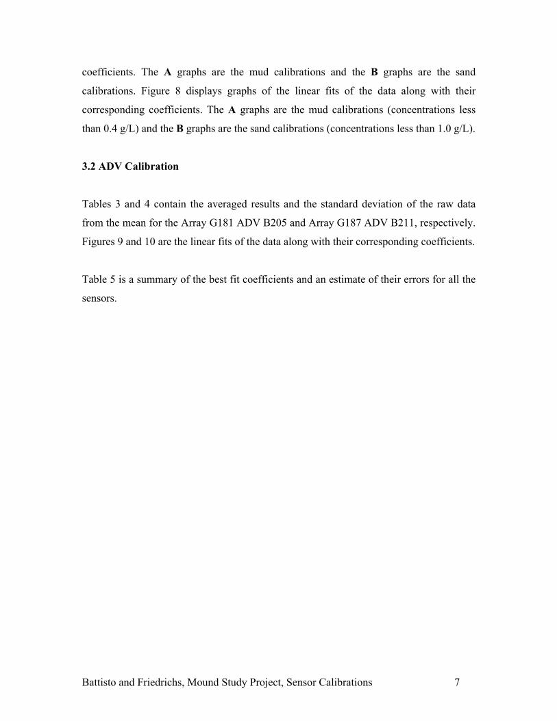
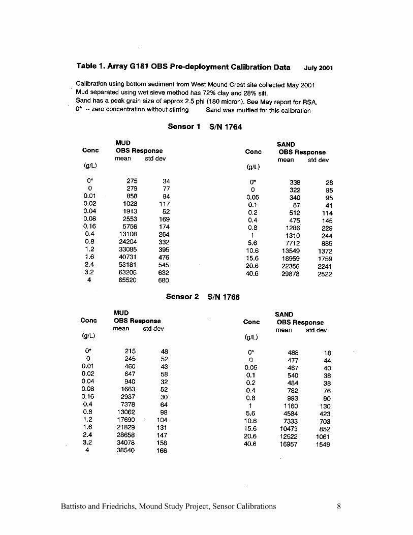
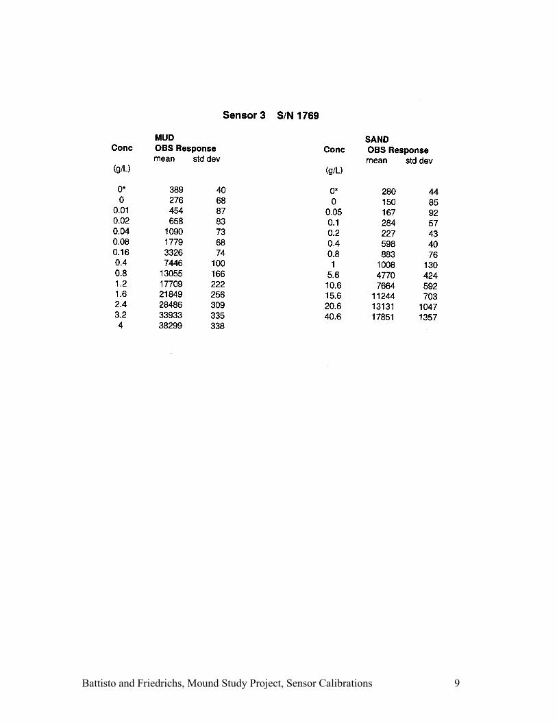
3.1 OBS Calibration

Table 1 contains the averaged results and the standard deviation of the raw data from the

mean for the Array G181 three OBS sensors’ mud and sand calibrations. Figures 5

displays graphs of the quadratic fit of the data along with their corresponding

coefficients. The A graphs are the mud calibrations and the B graphs are the sand

calibrations. Figures 6 displays graphs of the linear fits of the data along with their

corresponding coefficients. The A graphs are the mud calibrations (concentrations less

than 0.4 g/L) and the B graphs are the sand calibrations (concentrations less than 1.0 g/L).

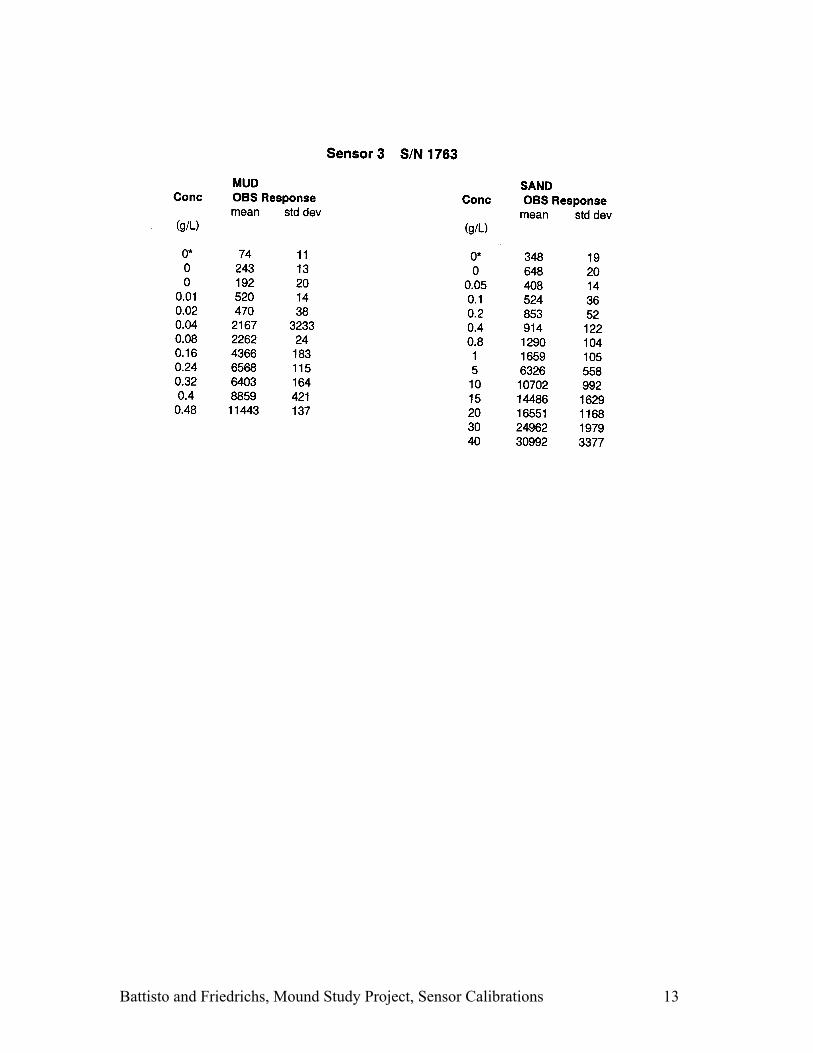
Table 2 contains the averaged results and the standard deviation of the raw data from the

mean for the Array G187 three OBS sensors’ mud and sand calibrations. Figure 7

displays graphs of the quadratic fits of the data along with their corresponding


coefficients. The A graphs are the mud calibrations and the B graphs are the sand

calibrations. Figure 8 displays graphs of the linear fits of the data along with their

corresponding coefficients. The A graphs are the mud calibrations (concentrations less

than 0.4 g/L) and the B graphs are the sand calibrations (concentrations less than 1.0 g/L).

3.2 ADV Calibration

Tables 3 and 4 contain the averaged results and the standard deviation of the raw data

from the mean for the Array G181 ADV B205 and Array G187 ADV B211, respectively.

Figures 9 and 10 are the linear fits of the data along with their corresponding coefficients.

Table 5 is a summary of the best fit coefficients and an estimate of their errors for all the

sensors.




0 05000 10000 15000 20000 25000 30000 35000 40000 0

0.5

1

1.5

2

2.5

3

3.5

4

4.5

Sensor 3 mean response

Mud

Cal

ibra

tion

Con

cent

ratio

n (g

/L)

y = 1.8e-009*x2 + 3.5e-005*x + 0.0042

Sensor 3 quadratic

0 10000 20000 30000 40000 50000 60000 700000

0.5

1

1.5

2

2.5

3

3.5

4

4.5


Mud

Cal

ibra

tion

Con

cent

ratio

n (g

/L)

y = 6.5e-010*x2 + 1.3e-005*x + 0.028

Sensor 1 quadratic

0 5000 10000 15000 20000 25000 30000 35000 40000 0

0.5

1

1.5

2

2.5

3

3.5

4

4.5


Mud

Cal

ibra

tion

Con

cent

ratio

n (g

/L)

y = 1.7e-009*x2 + 3.6e-005*x + 0.0083

Sensor 2 quadratic

0 5000 10000 15000 20000 0

10

20

30

40

50

60


San

d C

alib

ratio

n C

once

ntra

tion

(g/L

)

y = 1.2e-007*x2 + 0.00036*x + 0.14

Sensor 2 quadratic

0 5000 10000 15000 20000 0

5

10

15

20

25

30

35

40

45

50


San

d C

alib

ratio

n C

once

ntra

tion

(g/L

)

y = 1.1e-007*x2 + 0.00031*x + 0.27

Sensor 3 quadratic

0 5000 10000 15000 20000 25000 30000 0

5

10

15

20

25

30

35

40

45


San

d C

alib

ratio

n C

once

ntra

tion

(g/L

)

y = 4e-008*x2 + 0.00012*x + 0.37

Sensor 1 quadratic

Figure 5.1-5.3. Array G181 OBS sensor calibration graphs. Figures 1A – 3A are quadraticfits of the mud calibrations for sensors 1, 2, and 3, respectively. Figures 1B– 3B are thequadratic fits of sand calibrations for sensors 1, 2, and 3, respectively.

1A

3A

2A

3B

2B

1B


0 2000 4000 6000 8000 10000 12000 14000-0.05

0

0.05

0.1

0.15

0.2

0.25

0.3

0.35

0.4

0.45


Mud

Cal

ibra

tion

Con

cent

ratio

n (g

/L)

y = 3.1e-005*x - 0.012

Sensor 1 linear

0 1000 2000 3000 4000 5000 6000 7000 8000-0.05

0

0.05

0.1

0.15

0.2

0.25

0.3

0.35

0.4

0.45


Mud

Cal

ibra

tion

Con

cent

ratio

n (g

/L)

y = 5.6e-005*x - 0.013

Sensor 2 linear

400 500 600 700 800 900 1000 1100 1200-0.2

0

0.2

0.4

0.6

0.8

1

1.2


San

d C

alib

ratio

n C

once

ntra

tion

(g/L

)

y = 0.0014*x - 0.62

Sensor 2 linear

0 200 400 600 800 1000 1200 1400-0.2

0

0.2

0.4

0.6

0.8

1

1.2


San

d C

alib

ratio

n C

once

ntra

tion

(g/L

)

y = 0.00079*x - 0.14

Sensor 1 linear

0 1000 2000 3000 4000 5000 6000 7000 8000-0.05

0

0.05

0.1

0.15

0.2

0.25

0.3

0.35

0.4

0.45


Mud

Cal

ibra

tion

Con

cent

ratio

n (g

/L)

y = 5.6e-005*x - 0.019

Sensor 3 linear

0 200 400 600 800 1000 1200-0.2

0

0.2

0.4

0.6

0.8

1

1.2


San

d C

alib

ratio

n C

once

ntra

tion

(g/L

)

y = 0.0011*x - 0.18

Sensor 3 linear

1B

3B

2B

3A

2A

1A

Figure 6.1-6.3. Array G181 OBS sensor calibration graphs. Figures 1A – 3A are linear fits of the mud calibrations for sensors 1, 2, and 3, respectively. Figures 1B – 3B are linear fits of the sand calibrations for sensors 1, 2, and 3, respectively.




0 5000 10000 15000 20000 0 5000 10000 15000 20000 0 -0.1

0

0.1

0.2

0.3

0.4

0.5

0.6


Mud

Cal

ibra

tion

Con

cent

ratio

n (g

/L)

y = 2.2e-010*x2 + 2e-005*x - 0.0079

Sensor 1 quadratic

0 10000 20000 30000 40000 50000 60000-5

0

5

10

15

20

25

30

35

40

45


San

d C

alib

ratio

n C

once

ntra

tion

(g/L

)

y = 7.6e-009*x2 + 0.00028*x - 0.028

Sensor 1 quadratic

0 5000 10000 15000 20000 25000 30000 35000-10

0

10

20

30

40

50


San

d C

alib

ratio

n C

once

ntra

tion

(g/L

)

y = 1.3e-008*x2 + 0.00092*x - 0.53

Sensor 3 quadratic

0 10000 20000 30000 40000 50000-5

0

5

10

15

20

25

30

35

40

45


San

d C

alib

ratio

n C

once

ntra

tion

(g/L

)

y = 1e-008*x2 + 0.00032*x - 0.0024

Sensor 2 quadratic

0 5000 10000 15000 20000 25000-0.1

0

0.1

0.2

0.3

0.4

0.5

0.6


Mud

Cal

ibra

tion

Con

cent

ratio

n (g

/L)

y = - 5e-011*x2 + 2.4e-005*x - 0.009

Sensor 2 quadratic

0 2000 4000 6000 8000 10000 12000-0.1

0

0.1

0.2

0.3

0.4

0.5

0.6


Mud

Cal

ibra

tion

Con

cent

ratio

n (g

/L)

y = 2.1e-010*x2 + 4.2e-005*x - 0.013

Sensor 3 quadratic

Figure 7.1 – 7.3. Array G187 OBS sensor calibration graphs. Figures 1A – 3A are quadratic fits of the mud calibrations for sensors 1, 2, and 3, respectively. Figures 1B – 3B are quadratic fits of sand calibrations for sensors 1, 2, and 3, respectively.

1A

3B3A

2A 2B

1B


0 5000 10000 15000 20000 0 5000 10000 15000 20000 0 -0.1

0

0.1

0.2

0.3

0.4

0.5

0.6


Mud

Cal

ibra

tion

Con

cent

ratio

n (g

/L)

y = 2.4e-005*x - 0.014

Sensor 1 linear

0 5000 10000 15000 20000 25000-0.1

0

0.1

0.2

0.3

0.4

0.5

0.6


Mud

Cal

ibra

tion

Con

cent

ratio

n (g

/L)

y = 2.3e-005*x - 0.0072

Sensor 2 linear

0 2000 4000 6000 8000 10000 12000-0.1

0

0.1

0.2

0.3

0.4

0.5

0.6


Mud

Cal

ibra

tion

Con

cent

ratio

n (g

/L)

y = 4.4e-005*x - 0.015

Sensor 3 linear

0 500 1000 1500 2000 2500 3000-0.2

0

0.2

0.4

0.6

0.8

1

1.2


San

d C

alib

ratio

n C

once

ntra

tion

(g/L

)

y = 0.00038*x - 0.14

Sensor 1 linear

0 500 1000 1500 2000 2500-0.2

0

0.2

0.4

0.6

0.8

1

1.2


San

d C

alib

ratio

n C

once

ntra

tion

(g/L

)

y = 0.00047*x - 0.15

Sensor 2 linear

200 400 600 800 1000 1200 1400 1600 1800-0.2

0

0.2

0.4

0.6

0.8

1

1.2


San

d C

alib

ratio

n C

once

ntra

tion

(g/L

)

y = 0.00082*x - 0.36

Sensor 3 linear

3B

2B

1B

2A

3A

1A

Figure 8.1 – 8.3. Array G187 OBS sensor calibration graphs. Figures 1A – 3A are linear fits of the mud calibrations for sensors 1, 2, and 3, respectively. Figures 1B – 3B are linear fits of sand calibrations for sensors 1, 2, and 3, respectively.



-8000 -6000 -4000 -2000 0 2000 4000 6000 8000-80

-60

-40

-20

0

20

40

60

80

ADV response (divide by 100 for cm/sec)

Flu

me

curr

ent s

peed

(cm

/sec

)

B205 X AXIS y = 0.0097*x - 0.8

data linear

-5000 -2500 0 2500 5000-60

-40

-20

0

20

40

60


Flu

me

curr

ent s

peed

(cm

/sec

)

B211 X AXIS y = 0.01*x + 0.021

data linear

-5000 -2500 0 2500 5000-60

-40

-20

0

20

40

60


Flu

me

curr

ent s

peed

(cm

/sec

)

B211 Y AXIS y = 0.0099*x + 1.2

data linear

-8000 -6000 -4000 -2000 0 2000 4000 6000 8000-80

-60

-40

-20

0

20

40

60

80


Flu

me

curr

ent s

peed

(cm

/sec

)

B205 Y AXIS y = 0.0097*x - 0.05

data linear

Figure 9. Array G181 ADV B205 sensor calibration graphs. Graph A is the X axis linear fit of the data and B is the Y axis linear fit.

A

BA

B

Figure 10. Array G187 ADV B211 sensor calibration graphs. Graph A is the X axis linear fit of the data and B is the Y axis linear fit.


Table 5. Summary of Best Fit Coefficients and Estimates of Their Errors

CalibrationArray Sensor S/N Type A B C

G181 OBS 1 1764 MUD -0.028 ± 0.053 ( 1.30 ± 0.57 ) e -5 ( 6.50 ± 0.91 ) e -10 -0.0118 ± 0.0031 ( 3.1230 ± 0.0069 ) e -5

OBS 2 1768 0.008 ± 0.012 ( 3.61 ± 0.21 ) e -5 ( 1.7173 ± 0.0059 ) e -9 -0.0133 ± 0.0021 ( 5.6382 ± 0.0059 ) e -5

OBS 3 1769 0.004 ± 0.012 ( 3.55 ± 0.21 ) e -5 ( 1.762 ± 0.059 ) e -9 -0.0187 ± 0.0017 ( 5.5837 ± 0.0058 ) e -5

G181 OBS 1 1764 SAND 0.37 ± 0.42 ( 1.2 ± 1.1 ) e -4 ( 3.95 ± 0.43 ) e -8 -0.145 ± 0.076 ( 7.9 ± 1.0 ) e -4

OBS 2 1768 0.14 ± 0.41 ( 3.6 ± 1.9 ) e -4 ( 1.15 ± 0.12 ) e -7 -0.618 ± 0.070 ( 1.390 ± 0.097 ) e -3

OBS 3 1769 0.27 ± 0.40 ( 3.1 ± 1.8 ) e -4 ( 1.06 ± 0.11 ) e -7 -0.183 ± 0.051 ( 1.116 ± 0.092 ) e -3

G187 OBS 1 1761 MUD 0.0078 ± 0.0030 ( 2.05 ± 0.11 ) e -5 ( 2.16 ± 0.59 ) e -10 0.0144 ± 0.0043 ( 2.438 ± 0.039 ) e -5

OBS 2 1762 -0.0090 ± 0.0055 ( 2.39 ± 0.18 ) e -5 ( -5.1 ± 9.1 ) e -11-0.0072 ± 0.0046 ( 2.295 ± 0.048 ) e -5

OBS 3 1763 -0.013 ± 0.012 ( 4.21 ± 0.67 ) e -5 ( 2.1 ± 6.3 ) e -10 0.014 ± 0.010 ( 4.42 ± 0.20 ) e -5

G187 OBS 1 1761 SAND -0.03 ± 0.11 ( 2.80 ± 0.15 ) e -5 ( 7.64 ± 0.30 ) e -9 -0.14 ± 0.05 ( 3.84 ± 0.34 ) e -4

OBS 2 1762 0.00 ± 0.21 ( 3.21 ± 0.33 ) e -4 ( 1.01 ± 0.08 ) e -8 -0.151 ± 0.048 ( 4.687 ± 0.039 ) e -4

OBS 3 1763 0.53 ± 0.24 ( 9.22 ± 0.58 ) e -4 ( 1.26 ± 0.21 ) e -8 -0.361 ± 0.078 ( 8.19 ± 0.84 ) e -4

Concentration = A + B (Response) +C (Response)2


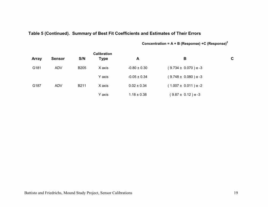
Table 5 (Continued). Summary of Best Fit Coefficients and Estimates of Their Errors

CalibrationArray Sensor S/N Type A B C

G181 ADV B205 X axis -0.80 ± 0.30 ( 9.734 ± 0.070 ) e -3

Y axis -0.05 ± 0.34 ( 9.748 ± 0.080 ) e -3

G187 ADV B211 X axis 0.02 ± 0.34 ( 1.007 ± 0.011 ) e -2

Y axis 1.18 ± 0.38 ( 9.87 ± 0.12 ) e -3

Concentration = A + B (Response) +C (Response)2

Documents

Mound Study Project Cape Fear, North Carolina Pre …cfried/reports/2003/Battisto_Friedrichs_2003_EHI... · Mound Study Project Cape Fear, North Carolina Pre-Deployment Calibration