Motor Vehicle Stocks, Scrappage, and Sales

* Alan Greenspan and Darrel Cohen

October 30, 1996

* Alan Greenspan is Chairman, Federal Reserve Board and Darrel Cohen is Economist, Federal Reserve Board, Washington, D.C. 20551.

This project owes a debt of gratitude to Don Mueller at R.L. Polk, Paul Sajak at American Automobile Manufacturers Association, Paul Harpel, Barbara Williams and Sue Ward at the Census Bureau, Bob Gish and Susan Liss at the Federal Highway Administration, Pat Hu at Oakridge National Laboratory, Everett Johnson at the Bureau of Economic Analysis, and Marti Johnson and Tom Welch at the Energy Information Administration. Also, we thank colleagues Bill Cleveland, Eric Engen, David Lebow, Wolf Ramm, Dan Sichel, Larry Slifman, Sandy Struckmeyer, David Wilcox, and, especially, Glenn Follette for constructive suggestions; we also thank Jeff Campione, Vandy Howell, and Eliot Maenner for their research assistance.

The views expressed are those of the authors and do not necessarily represent those of the entire Board of Governors or the staff of the Federal Reserve System.

Motor Vehicle Stocks, Scrappage, and Sales

I. Introduction

The motor vehicle sector remains an important part of the U.S. macroeconomic

landscape. Sales of new motor vehicles and accessories currently account for roughly 25

percent of personal consumption expenditures on durables, while production of motor

vehicles and parts accounts for about 5 percent of manufacturing production. In addition,

the sector has exhibited strong procyclical behavior; this is evidenced by a statistically

significant contemporaneous correlation of the quarterly growth rates of motor vehicle

sales and real GDP of about 0.5 over the past four decades, a correlation that has risen

to about 0.6 in the 1990s.

This paper offers a new framework for analyzing aggregate sales of new motor

vehicles that incorporates separate models for the change in the vehicle stock and for the

rate of vehicle scrappage. Because this approach requires only a minimal set of

assumptions about demographic trends, the state of the economy, consumer "preferences",

and vehicle retirements, it is shown to be especially useful as a macroeconomic 1 forecasting tool. In addition, a new historical annual time series estimate of motor

vehicle stocks in the United States is presented. In constructing this series, particular

attention is paid to the problems with existing data on vehicle stocks and scrappage.

Such efforts are based in part on the existence of a rare data set that provides direct

__________ 1. This paper contains an updated and extended version of the Townsend-Greenspan model’s motor vehicle sector. Further, the general approach of analyzing vehicle demand in terms of scrappage and of the change in vehicle stocks can be traced back to the work of P. de Wolff (1938) and of C.F. Roos and Victor Von Szeliski (1939).

-2-

2 evidence of the manner in which a capital good is retired over time. In contrast,

most evidence on the depreciation of physical assets is inferred from prices in markets

for used assets, such as Wykoff (1970).

Much of the subsequent discussion can be organized around the definition that

equates new vehicle sales to the change in the vehicle stock plus vehicle scrappage.

Further, scrappage can be defined in terms of two components. The first component is

"engineering" scrappage and reflects physical or "built-in" deterioration of the type

discussed in Richard Parks (1977, 1979); under this view, scrappage reflects physical wear

and tear that increases with vehicle age or use, although by an amount that varies with

model year (i.e., with differences in built-in durability). The second component is

labelled "cyclical" scrappage and reflects primarily the marked tendency of scrappage to

move in a procyclical manner, but also reflects the prices of new vehicles, repairs, and

gasoline. Thus, new sales can be expressed as follows:

Sales = ∆V + EngScrap + CycScrap (1) t t t t

where Sales denotes the rate of new sales of motor vehicles during period t, V denotes t the total stock of motor vehicles at the end of the period, EngScrap denotes the rate of

engineering scrappage during the period, and CycScrap denotes the rate of cyclical

scrappage. In practice, there are separate equations for cars and trucks.

It should be noted that equation 1 does not necessarily say anything about the

causal relationships among the various pieces. For example, it does not say that

scrappage "causes" new vehicle sales. It is possible, of course, that an "exogenous"

increase in scrappage (for example, due to engineering failures or to an economic boom)

__________ 2. More precisely, we observe the fraction of the initial stock of a given model year remaining on the road as of July 1 of successive years. The stock of any given model year is the aggregation over all domestically-made and foreign-made vehicles; the total stock is disaggregated into car and truck components.

-3-

leads to or causes an increase in new sales. This could occur if the owners of the

scrapped vehicles simply buy new vehicles. It also could occur if the owners demand

replacement used vehicles, which pushes up the price of used vehicles relative to the

price of new vehicles, and hence ultimately increases the demand for new vehicles.

Conversely, an exogenous increase in the demand for new vehicles may cause an increase in

scrappage if the new vehicle demand results in an increase in the supply of used vehicles

and hence a decline in relative used vehicle prices. We simply contend that equation 1 is

a useful way of organizing our thinking about new vehicle sales and of generating a

forecast of them.

Subsequent sections describe in detail how each term on the right hand side of

equation 1 is constructed. In the process, we identify conceptual problems with the

standard data on the stock of motor vehicles in operation and vehicle scrappage rates as

published by R.L. Polk & Co. and the American Automobile Manufacturers Association (AAMA).

In addition, alternative data sources are explored, and separate estimates of household,

business, and government vehicle stocks are presented.

II. The Stock of Motor Vehicles

This section is divided into two parts. In the first, the underlying Polk data and

their conceptual limitations are discussed. In the second, the method of forecasting ∆V

in equation 1 is described.

A. Data Preliminaries

Both Polk and AAMA publish, as they label it, the outstanding stock of "cars in use" 3 and "trucks in use" in the United States as of July 1 of each year. In fact, each

series is nothing more than the number of vehicles registered as of July 1. The data are

__________ 3. The stock of trucks is comprised of light, medium, and heavy trucks.

-4-

assembled in matrix form; row i presents the stock of model-year i registrations as of

July 1 of successive years and column j presents the stock of registrations of all model

years as of July 1 of year j.

The concepts of "vehicles in use" and "vehicles registered" are closely related, but

not identical; in practice, vehicles in use as of July 1 of a given year are overstated by

the number of vehicles registered but scrapped (because of old age or accident) during the

prior year. The main underlying problem is that scrapped vehicles are not effectively

deleted from the individual state registrations data until they fail to be re- 4 registered. For example, a car registered on May 1, 1991 would be counted as part of

"cars in use" as of July 1, 1991 even if it were destroyed in an accident on May 2; this

car would not be re-registered in May 1992 and, thus, its scrappage would not be captured 5 in the cars-in-use statistics until July 1, 1992.

It follows from this discussion that if a vehicle is truly in existence (and

registered) on July 1 of year t-1 then it will appear in the Polk registrations data as of

__________ 4. Polk and AAMA do not publish true scrappage rates but, rather, vehicles not re- registered; this figure is derived as the difference between the the flow of new registrations during the 12 months ending on June 30 of a given year and the change in the stock of registrations between July 1 of the given and prior year. Our estimates of vehicle scrappage use this approach but with our estimate of the change in the stock of vehicles (discussed below) substituting for Polk’s change in the stock of registrations. The Polk data allow for an alternative method of computing vehicles not re-registered. Specifically, Polk calculates the number of vehicles of a given model year registered as of June 30 of each year; thus, total vehicles not re-registered during a year may be computed by adding up the year-to-year reductions in registrations for each model year. The relationship between the two methods is examined in Appendix 1.

5. One colleague has questioned whether this is really a problem, conjecturing that if the license plates of the car destroyed by accident are transferred to a new car, then the state registrations data would show only one car registered. Based on information supplied by an official of California’s Department of Motor Vehicles, this possibility can be rejected. In California, irrespective of the transfer of plates, the destroyed car’s registration stays in the computer system until the following year when it is not re-registered. Thanks to the DMV official who also helped to clarify other aspects of the subsequent discussion.

-5-

July 1 of year t. Alternatively, if a vehicle is in the Polk registrations data as of

July 1 of year t then it truly must have been on the road as of July 1 of year t-1, unless

the vehicle was sold new between July 1 of year t-1 and year t. This insight allows for

the construction of the "true" stock of vehicles as follows:

V(t-1) = R(t) - [M(t,t) + M(t-1,t)] + (.99)F(t-1) (2)

where V(t-1) denotes the "true" stock of vehicles as of July 1 of year t-1; R(t) denotes

the Polk stock of vehicle registrations as of July 1 of year t; M(t,t) denotes the Polk

stock of registrations of model-year t vehicles as of July 1 of year t; M(t-1,t) denotes

the Polk stock of registrations of model-year t-1 vehicles as of July 1 of year t; F(t-1)

denotes the flow of new registrations of model year t-1 vehicles recorded over the nine 6 months ending on June 30 of year t-1.

This relationship is best illustrated with an example. The true stock of vehicles

on the road as of July 1, 1990 [i.e., V(1990)], for example, equals the Polk stock of

registrations as of July 1, 1991 minus the number of 1991 and 1990 model-year

registrations as of July 1, 1991 plus the number of new 1990 model-year vehicles 7 registered over the nine months ending on June 30, 1990 (times 0.99).

__________ 6. An implication of the incorrect estimate of the stock of vehicles as published by Polk and AAMA is that their estimates of the mean and median age of the vehicle stock also are incorrect. Using our corrected estimates of cars, for example, we find that the average and median ages each are roughly 0.4 year lower than the Polk/AAMA estimates in each year during the 1980s; this implies that the alternative estimates of the increase in the mean and median ages over this period are quite similar.

7. This assumes that new 1990 model-year vehicle sales began in October, 1989. New model- year t vehicle sales generally have begun in October of the prior year; construction of our historical vehicle stock series assumes an October 1 starting date for each model-year vehicle. Also, we multiply the number of new vehicles registered (over the nine months between October 1 and June 30) by 0.99 to allow for the small amount of scrappage that occurs, according to the Polk data, in the first year that vehicles are on the road.

-6-

The stock of model-year 1991 registrations [i.e., M(1991,1991)] is subtracted out

because 1991 model-year sales began in earnest in October 1990, which is after July 1, 8 1990. Also, the stock of registrations of 1990 model-year vehicles as of July 1, 1991

[i.e., M(1990,1991)] is subtracted out because some new sales of 1990 model-year vehicles

took place after July 1, 1990 (and thus were not on the road then). However, some new

1990 models were on the road and these are captured by the final term (i.e., by

registrations of new 1990 model-year vehicles recorded over the nine months ending June

30, 1990); the final term is multiplied by 0.99, the fraction of the new 1990 models

assumed to remain on the road as of June 30, 1990.

Estimates of the total stock of cars and trucks for the period 1973 to 1991 are

presented in the first column of table 1. In addition to the measurement problems

discussed above, the Polk data are subject to a few other conceptual problems as well, the

most important being the possibility of double counting. A discussion of this problem,

as well as its elimination for the first time in Polk’s 1992 vehicle stock data, is

contained in appendix 2 (which also includes discussion of alternative data sources).

B. Forecasting Vehicle Stocks

As a preliminary exercise to forecasting the stocks of cars and trucks, the total

stock of vehicles is divided into the stock owned by business and government and the stock

available to households. Polk data (modified in accordance with equation 2) and Census

Bureau data on the household stock are combined for this purpose; the Census data are

described in appendix 2.

As shown in table 1, the Census estimate of the household stock (for available

years) is subtracted from our estimate of the total stock for the corresponding historical

period. The resulting series for the stock of business and government vehicles is then

__________ 8. In addition, a small number of registrations of 1992 models [M(1992,1991)] are subtracted out.

-7-

"smoothed". Smoothing is necessary because we do not think that the stock varies as much

over time as suggested by the raw data and because ultimately we want a sensible estimate

of the change in the stock. As seen in column 4, the "smoothed" business and government

stock increased only a bit over the past two decades. Finally, this smoothed series is

subtracted from the total stock to produce a smoothed series for the household stock of

vehicles.

To forecast the household stock of cars and trucks, Census vehicle data are used

again. The following equation underlies the calculations:

V = (# HH’s)(% of HH’s owning)(Avg # of vehicles per HH that) HH vehicle own a vehicle

The stock is given as the product of the number of households, the fraction of households

owning at least one vehicle, and the average number of vehicles per household that owns a

vehicle. In fact, there are separate equations used for forecasting the stock of cars and

the stock of light trucks. The stock of household vehicles thus is modeled to depend on

demographics as well as on factors related to consumer preferences. The strength of this

approach is that it is based on a few easily forecastable factors.

The first term on the right hand side, the number of households, is estimated 9 through 1995 by the Census Bureau. The second term, the fraction of households owning

a vehicle, is shown in the first column of table 2 in the case of cars and in the second

column in the case of trucks. Census data extend only through 1993 and forecasts for

1994, 1995, and 1996 are shown in the table; the fraction is assumed to be essentially

__________ 9. More precisely, household estimates through 1991 are taken directly from the Census’ American Housing Survey, the source also used for details of household car and truck ownership. For 1992 to 1995, the 1991 estimate is assumed to grow by the same amount as Census’ estimate of households found in the Current Population Reports, Series P-60; over this period, the number of households has grown at an average rate of about 1.25 million per year, the increase assumed for 1996.

-8-

10 constant in the case of cars and to trend up in the case of trucks. The final term on

the right hand side, in the case of cars, can be expanded as follows:

Avg # cars per HH = 1*(% owning exactly 1) + 2*(% owning exactly 2) + 3.1*(% owning at least 3)

The analogous expression for trucks is given by:

Avg # trucks per HH = 1*(% owning exactly 1) + 2.1*(% owning at least 2)

In the previous two equations it is assumed that the average number of cars held by

households with at least 3 cars is 3.1, and the average number of trucks held by

households with at least 2 trucks is 2.1; however, any number between 3.0 and 3.2 in the

case of cars and between 2.0 and 2.2 in the case of trucks is plausible. Fortunately, our

subsequent forecasts of changes in vehicle stocks are insensitive to such variations. In

addition, as shown in table 2, other components of the last two equations are relatively

easy to forecast. In the case of cars, each of the components has been roughly constant

over the last decade. In the case of trucks, the components have grown steadily since the

mid-1980s. The values in table 2 for 1990 and 1992 (years in which the Census survey was

not conducted) are interpolations between adjacent observed values. The forecast values

for 1994 and 1995 are linear extrapolations, based on the average experience since the

mid-1980s.

In sum, we now are able to forecast the household stock of vehicles and, thus, the

first term on the right hand side of equation 1 (making a suitable assumption about

__________ 10. Conceivably these fractions, as well as those discussed subsequently, could be modeled in terms of relative price and demographic movements instead of the exogenous trends used by us.

-9-

changes in the business and government stocks, as discussed below). We turn to the

construction of the other two terms.

III. Engineering Scrappage

As an empirical proposition, very few vehicles are scrapped during the first three

years of life. During this period most scrappage presumably results from accidents; in

later years, scrappage also results from an economic decision by the owner to replace an

increasingly unreliable vehicle with a more reliable alternative means of transportation 11 (such as a newer car, public transportation, etc.). In making the scrappage decision,

the owner weighs the benefits--scrappage value plus foregone headaches associated with

unreliability plus foregone maintenance expenses--against the costs of alternative means

__________ 11. We have attempted to collect direct evidence on who makes the scrappage decision. We conducted a telephone survey of six auto scrappage businesses in the Washington, D.C. area as well as several industry associations including the Insurance Information Institute, the National Insurance Crime Bureau (NICB), the American Salvage Pool Association, CCC Information Services, and the Automotive Recyclers Association (ARA). Unfortunately, not much quantitative information is available. The two fairly reliable pieces of information for recent years are that (i) roughly 1 million vehicles per year are stolen and lost from the U.S. vehicle stock because they are illegally exported, chopped, stripped, burned, etc. (National Insurance Crime Bureau) and (ii) about 2.5 million vehicles per year are declared total losses by the insurance industry (CCC Information Services). Together scrappage for these two reasons adds up to about 3.5 million vehicles per year (ignoring the possibility of some double counting), roughly 8 million units less than the aggregate annual U.S. scrappage rate in the 1990s. If these figures are even roughly correct, then the majority of scrappage is undertaken by individual owners (quite possibly with no collision insurance) who either abandon their vehicles or tow them to the junkyard, or it is undertaken by auto dealers (who get trade-in vehicles not worth the cost of fixing up for resale). The ARA 1995 annual membership survey, for example, indicates that car dealers do scrap vehicles, but infrequently. Thus, by process of elimination, it appears that the major suppliers of scrapped vehicles, at least in recent years, are individual owners; this contrasts with previous academic work, such as Walker (1968), in which auto dealers are viewed as the agents making the scrappage decision.

-10-

12 of transportation. Maintenance outlays generally increase with vehicle age, in part

because of engineering-related or built-in limitations to durability of the type described

in Parks (1977, 1979); that is, scrappage results partly from age-dependent physical wear

and tear, and we refer to this as engineering scrappage.

Moreover, for any given vehicle age, maintenance outlays rise with intensity of use,

which itself is assumed to depend on such factors as the price of gasoline and real

income. Real income also may enter as an independent determinant of scrappage to the

extent that vehicle reliability is a normal good. Indeed, as discussed in the next

section, the aggregate scrappage rate has a pronounced cyclical pattern, falling sharply

during recessions and rebounding during recoveries.

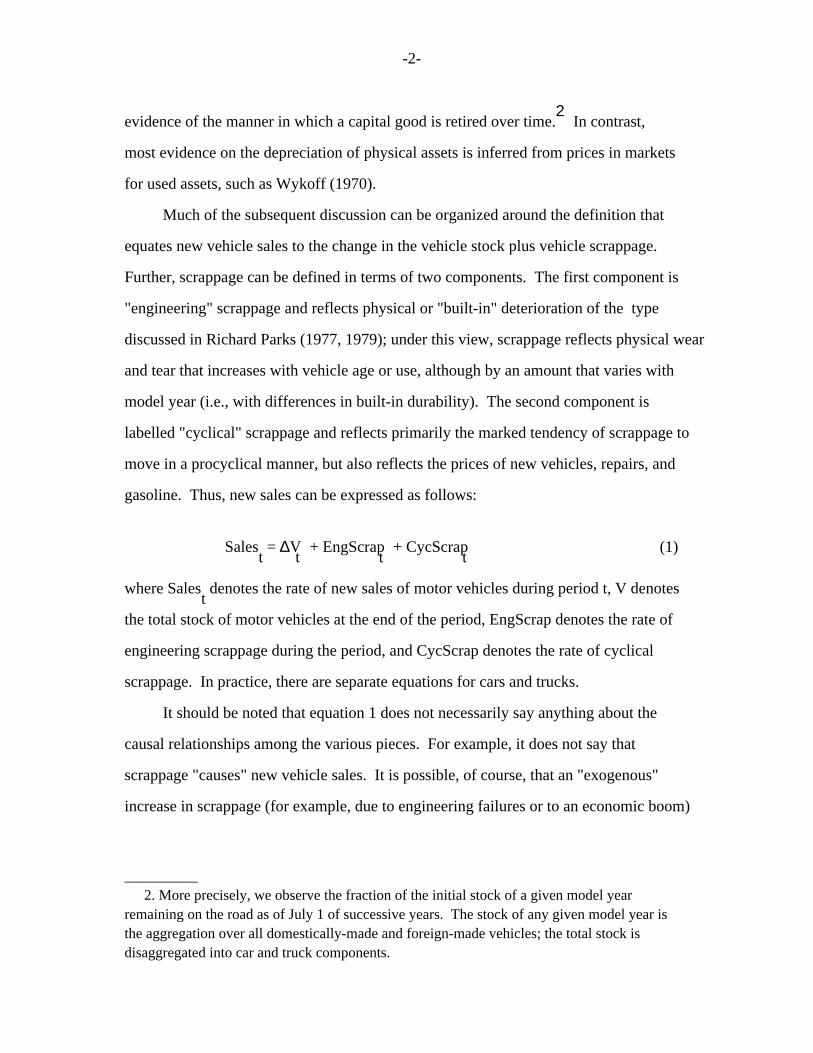
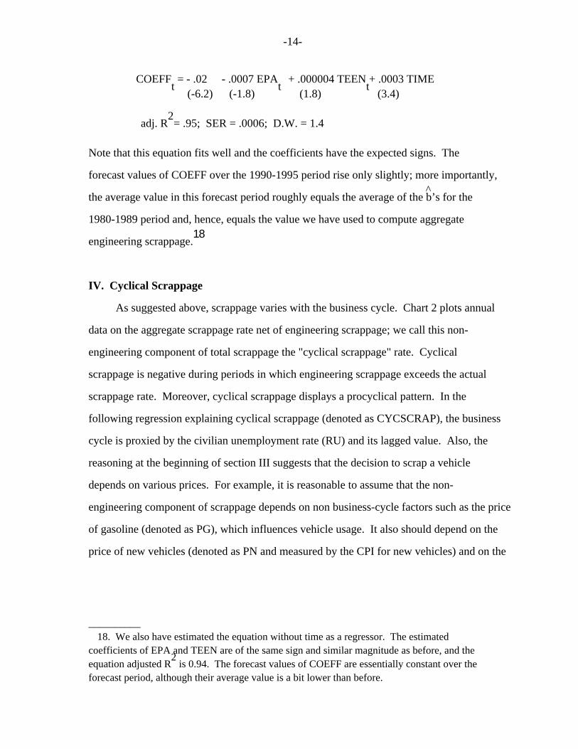
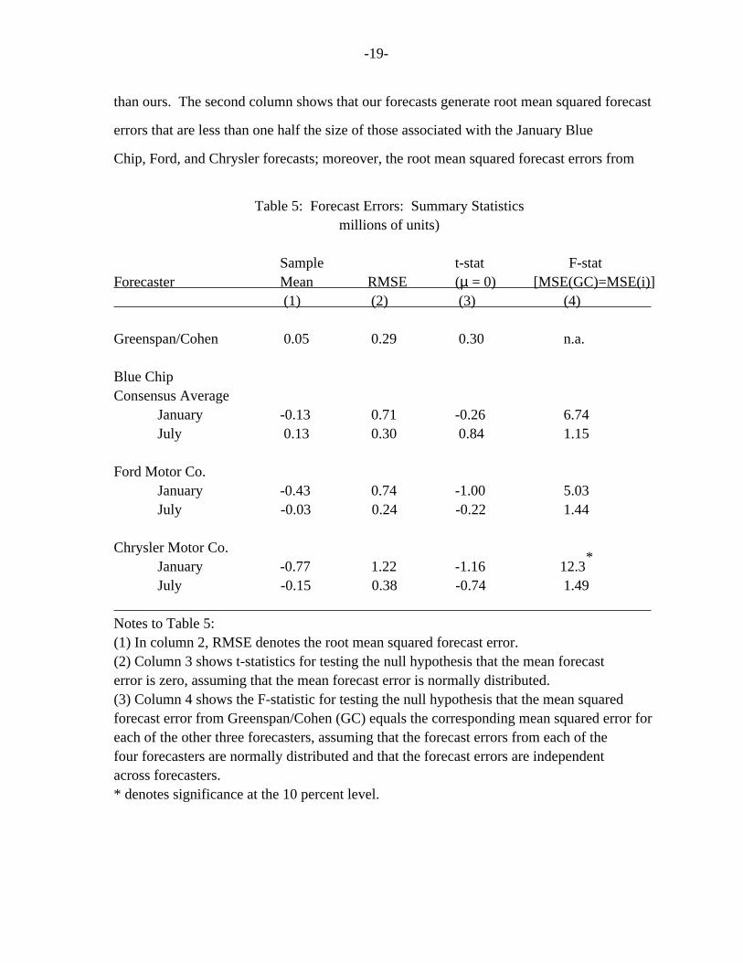
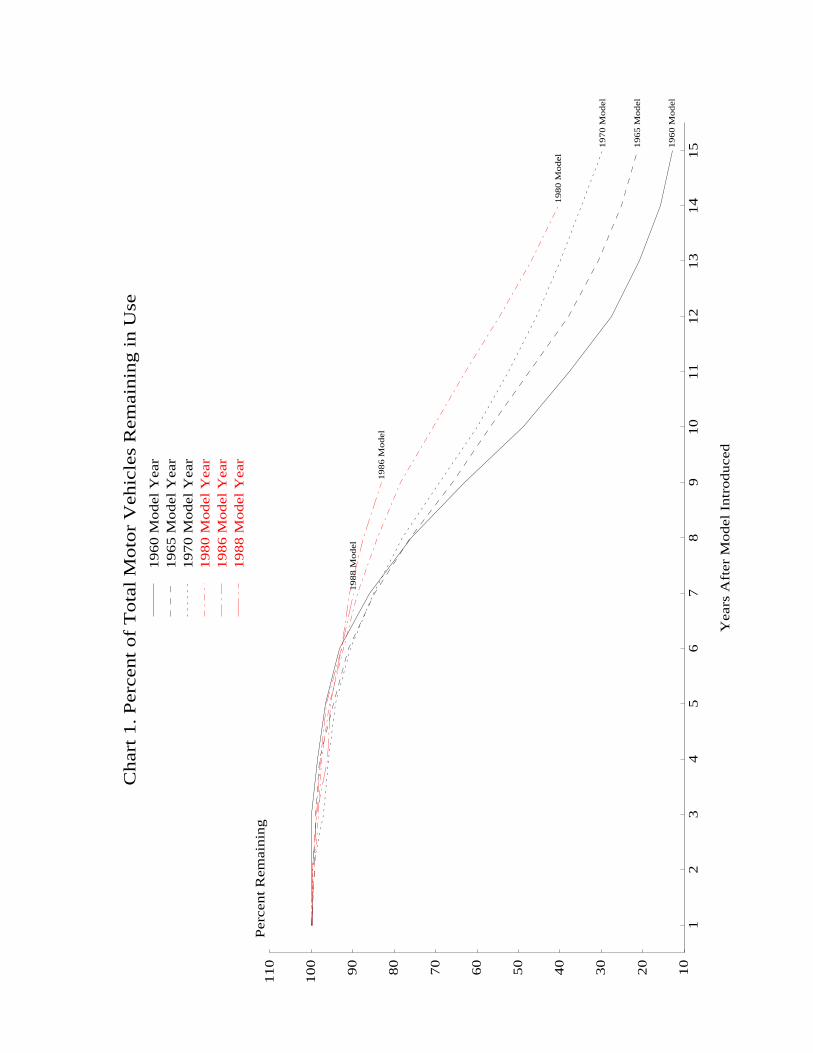
Chart 1 shows the percent of initial vehicle registrations remaining plotted against

vehicle age for several model years. Typically, as noted above, registrations (and hence

scrappage) are flat for the first few years, decline at an increasing rate for several

years, and flatten out again at age 12 or 13. Also, there appears to have been

improvement in vehicle durability from the early 1960 vintages to the late 1970 ones as

evidenced by the outward shift in the schedules. Indeed, the age at which only 50 percent

of the initial stock of a given model year car remains on the road increased from 10 years

for 1960-1963 models to 11 years for 1964-1971 models to 12 years for 1972-1976 models to 13 13 years for 1977-1979 models. The limited evidence for vehicles made through the

early 1980s suggests that the improvements in durability either stopped or slowed down

significantly around 1980; the age at which only 50 percent of the initial stock of 1980,

__________ 12. This is not intended as a precise statement of first-order conditions. For a more formal treatment, see Parks (1977, 1979) and James Berkovec (1985) who compare the benefits of scrapping discussed above to the vehicles’s value in use as measured by its price.

13. Based on such a measure, trucks have been more durable than cars since the beginning of our sample. More than 50 percent of the initial stock of every model year truck since the early 1960s has remained on the road after 15 years, the maximum age reported by Polk.

-11-

1981, and 1982 model year cars remained on the road fell back to 12 years (these are the 14 last vintages for which enough longevity data exist for such calculations). Based

on even more limited information, it appears that durability once again improved for model

years 1983-1986 but dropped back for model years 1987-1989 to levels experienced in the

late 1970s (see Chart 1 for model years 1986 and 1988).

Formally, we capture engineering scrappage by estimating the following pooled

regression:

2 2 2 3 ln y = a + b t + b t + . . . + b t + ct + u it 1 60 2 61 30 89 it

where y denotes the fraction of vehicles of model year i remaining at age t (derived it from Polk registrations data). Because scrappage is essentially zero in the first three

years after a model is introduced, age is assumed to begin in the fourth year after

introduction; age ends in the fifteenth year after introduction, the final year covered by 2 the Polk data. The column vectors, t (i=1960, . . ., 1989), each have 309 elements. For i example, in transposed form: 2 t = (1,4,9,. . . ,144,0,. . . . . . . . . . . . . . . . . 0); 1960 2 t = (0, . . . . . . . .,0,1,4,9, . . .,144,0, . . . ,0); and so on. 1961 3 The column vector, t , in transposed form is given by:

3 t = (1,8,27, . . .,1728,1,8,27, . . .,1728, . . . . . . . .).

__________ 14. This evidence makes it hard to assess the common perception that recent vintages of cars have been better built: there is virtually no evidence on durability for cars built in the 1990s and the evidence for the 1980s is mixed. While it is true that the average age of the stock of cars increased in the early 1990s after being constant over the last half of the 1980s, this uptick in the average age appears to be due to technological improvements of 1983- 1986 model-year cars, rather than improvements in late 1980s model-year cars.

-12-

2 -kt The functional form is motivated by the normal density function (y = Ae ) which, in

broad terms, appears to fit the curves in Chart 1 well (for t > 0) and because it ensures

that forecasts of the fraction of vehicles remaining of any given model year goes to zero. However, experimentation suggested that the normal form generated too few very old cars, 15 3 i.e., the tail was not "thick" enough. To attenuate this problem, a t term was added as a regressor and assumed to have the same effect across the model years. The regression

results are presented in table 3. The overall equation fit is extremely good, and all ^ ^ ^ estimated coefficients are significant. The b s generally increase from b to b and then i 1 20 ^ fluctuate within a moderate band about the b value, reflecting the apparent changes in 20 vehicle durability described above.

The estimated equation is used for out-of-sample forecasts of the number of vehicles

remaining of each vintage through model year 1989. For subsequent model years, the same ^ estimated equation is used under the assumption that the b for each model year 1990 and 16 beyond equals the average value for the 1980-1989 model years. We present some

evidence supporting this assumption below. However, it should be noted that, strictly

speaking, this assumption implies that vehicle durability has not changed since the 1980-

1989 period; thus, our forecast of engineering scrappage is overstated if vehicle

durability has improved in the 1990s.

__________ 15. This was determined by predicting the aggregate number of aged vehicles remaining in a few specific years using two econometric specifications (an aged car is defined as one that is more than 15 years old). One specification is that shown above, while the other suppresses 3 the t term (i.e., the other uses the normal form). The prediction from the former is closer to the official Polk estimate of the number of aged vehicles in the same years.

16. The resulting forecasts of aggregate engineering scrappage are lagged one year to reflect the timing problems with the Polk data discussed in section II.A above. For example, the aggregate engineering scrappage for 1990 truly represents engineering scrappage in 1989.

-13-

Moreover, alternative plausible assumptions about vehicle durability in the early

1990s can have large effects on the estimates of aggregate engineering scrappage. For ^ example, if the b for model years subsequent to 1989 is assumed to rise at the average

change in the estimated coefficient values over the 1960-1979 period (a period of

virtually continuous improvement in vehicle durability), the estimate of aggregate

engineering scrappage would be about 0.2 million units lower in 1995 than the estimate ^ using a constant b. ^ Because of the sensitivity of the scrappage estimates to assumptions about b, we

attempted to model the estimated coefficients. These coefficients, as measures of vehicle

durability (or more precisely as measures of the vertical position of curves such as those

in chart 1), are posited to depend on EPA new vehicle emission standards. These standards

became increasingly stringent between the late 1960s and early 1980s and remained roughly

unchanged through the 1980s. We measure stringency by the inverse of the allowable number 17 of grams of hydrocarbons per mile. As the standards have become more demanding they

have become increasingly costly to satisfy, implying that vehicle scrappage should be more

rapid than in the absence of the standards.

The coefficients also are posited to depend on the number of teenagers (between 16

and 19 years old), assuming that scrappage of old vehicles is delayed to provide ^ transportation for these young drivers. Thus, in a regression of the b’s (denoted as

COEFF) on the EPA stringency measure (denoted as EPA) and on the number of teenagers

(denoted as TEEN), we expect the coefficient of the former to be negative and the

coefficient of the latter to be positive. The results of such a regression (also

including a linear time trend) using OLS over the period 1960 to 1989 are as follows (with

t-statistics in parenthesis):

__________ 17. The stringency of the standards for carbon monoxide and nitrogen oxides over time is quite similar to those for hydrocarbons.

-14-

COEFF = - .02 - .0007 EPA + .000004 TEEN + .0003 TIME t t t (-6.2) (-1.8) (1.8) (3.4)

2 adj. R = .95; SER = .0006; D.W. = 1.4

Note that this equation fits well and the coefficients have the expected signs. The

forecast values of COEFF over the 1990-1995 period rise only slightly; more importantly, ^ the average value in this forecast period roughly equals the average of the b’s for the

1980-1989 period and, hence, equals the value we have used to compute aggregate 18 engineering scrappage.

IV. Cyclical Scrappage

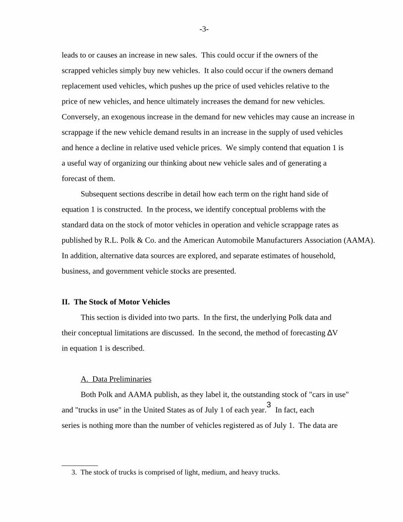
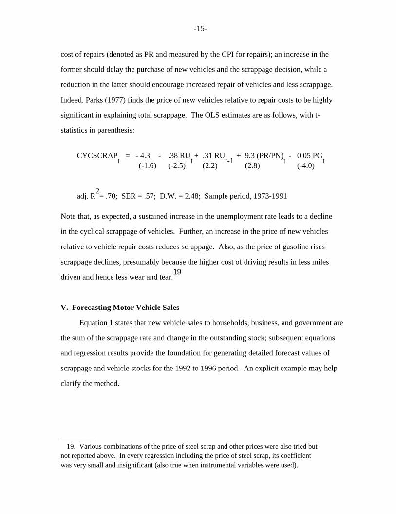
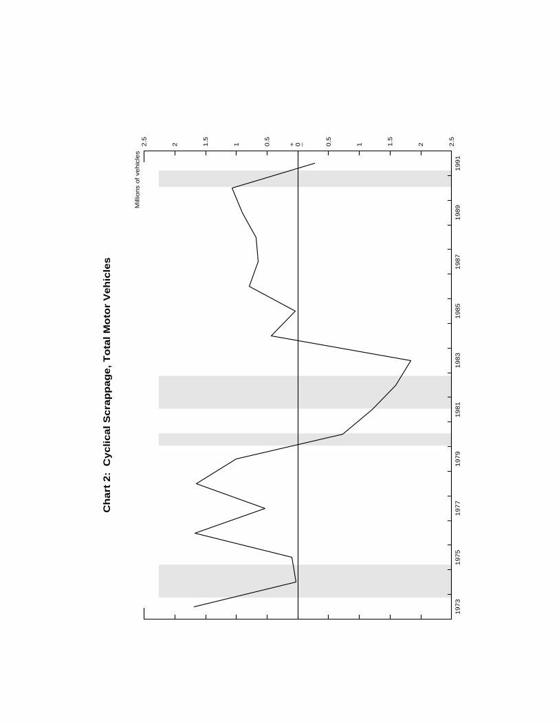
As suggested above, scrappage varies with the business cycle. Chart 2 plots annual

data on the aggregate scrappage rate net of engineering scrappage; we call this non-

engineering component of total scrappage the "cyclical scrappage" rate. Cyclical

scrappage is negative during periods in which engineering scrappage exceeds the actual

scrappage rate. Moreover, cyclical scrappage displays a procyclical pattern. In the

following regression explaining cyclical scrappage (denoted as CYCSCRAP), the business

cycle is proxied by the civilian unemployment rate (RU) and its lagged value. Also, the

reasoning at the beginning of section III suggests that the decision to scrap a vehicle

depends on various prices. For example, it is reasonable to assume that the non-

engineering component of scrappage depends on non business-cycle factors such as the price

of gasoline (denoted as PG), which influences vehicle usage. It also should depend on the

price of new vehicles (denoted as PN and measured by the CPI for new vehicles) and on the

__________ 18. We also have estimated the equation without time as a regressor. The estimated coefficients of EPA and TEEN are of the same sign and similar magnitude as before, and the 2 equation adjusted R is 0.94. The forecast values of COEFF are essentially constant over the forecast period, although their average value is a bit lower than before.

-15-

cost of repairs (denoted as PR and measured by the CPI for repairs); an increase in the

former should delay the purchase of new vehicles and the scrappage decision, while a

reduction in the latter should encourage increased repair of vehicles and less scrappage.

Indeed, Parks (1977) finds the price of new vehicles relative to repair costs to be highly

significant in explaining total scrappage. The OLS estimates are as follows, with t-

statistics in parenthesis:

CYCSCRAP = - 4.3 - .38 RU + .31 RU + 9.3 (PR/PN) - 0.05 PG t t t-1 t t (-1.6) (-2.5) (2.2) (2.8) (-4.0)

2 adj. R = .70; SER = .57; D.W. = 2.48; Sample period, 1973-1991

Note that, as expected, a sustained increase in the unemployment rate leads to a decline

in the cyclical scrappage of vehicles. Further, an increase in the price of new vehicles

relative to vehicle repair costs reduces scrappage. Also, as the price of gasoline rises

scrappage declines, presumably because the higher cost of driving results in less miles 19 driven and hence less wear and tear.

V. Forecasting Motor Vehicle Sales

Equation 1 states that new vehicle sales to households, business, and government are

the sum of the scrappage rate and change in the outstanding stock; subsequent equations

and regression results provide the foundation for generating detailed forecast values of

scrappage and vehicle stocks for the 1992 to 1996 period. An explicit example may help

clarify the method.

__________ 19. Various combinations of the price of steel scrap and other prices were also tried but not reported above. In every regression including the price of steel scrap, its coefficient was very small and insignificant (also true when instrumental variables were used).

-16-

To generate an estimate of new sales over the year ending on June 30, 1995, begin by

substituting the 1995 parameter values from table 2 and a Census estimate for total

households of 100.6 million into the equations in part B of section II. The implied

estimate of the household stock of cars is 124.9 million units and the estimate of trucks

is 46.1 million units, for a total of 171.0 million units. Similar calculations for 1994

yield a figure of 167.6 million units, implying a 3.4 million unit increase in the total

household vehicle stock between the two years. It is assumed that there is no change in

the stock of business and government vehicles (i.e., that the rate of new sales of

business and government vehicles equals their rate of scrappage).

An estimate of the rate of engineering scrappage of household, business, and

government vehicles is the calculated value implied by the engineering scrappage

regression described in section III (note that separate estimates for households,

businesses, and governments are not available). Specifically, for each model year

beginning in 1960 the regression is used to calculate the number of vehicles of that

vintage remaining in 1994 and 1995, with the difference representing the engineering

scrappage rate in 1995 of that particular vintage. The rates for the different vintages

are added together to get an aggregate estimate of 11.1 million units in 1995.

The rate of cyclical scrappage of household, business, and government vehicles is

calculated from the cyclical scrappage regression reported in section IV. In 1995, the

cyclical scrappage rate is calculated to be 0.8 million units.

Thus, assuming no change in the stock of business and government vehicles, the above

calculations substituted into equation 1 imply that new sales of vehicles in the year

ending June 30, 1995 should have been 15.3 million units (= 3.4 + 11.1 + 0.8); this

compares to actual sales of 15.3 million units (averaged over the four quarters ending in

1995 Q2).

-17-

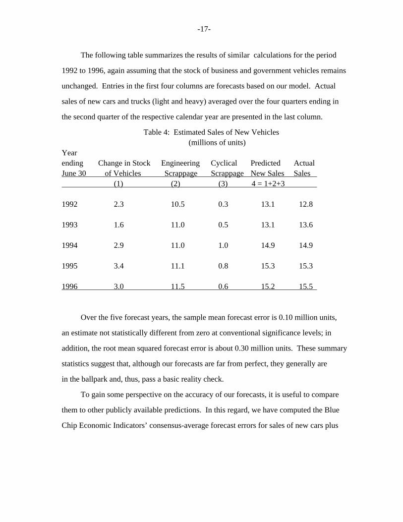
The following table summarizes the results of similar calculations for the period

1992 to 1996, again assuming that the stock of business and government vehicles remains

unchanged. Entries in the first four columns are forecasts based on our model. Actual

sales of new cars and trucks (light and heavy) averaged over the four quarters ending in

the second quarter of the respective calendar year are presented in the last column.

Table 4: Estimated Sales of New Vehicles (millions of units) Year ending Change in Stock Engineering Cyclical Predicted Actual June 30 of Vehicles Scrappage Scrappage New Sales Sales (1) (2) (3) 4 = 1+2+3

1992 2.3 10.5 0.3 13.1 12.8

1993 1.6 11.0 0.5 13.1 13.6

1994 2.9 11.0 1.0 14.9 14.9

1995 3.4 11.1 0.8 15.3 15.3

1996 3.0 11.5 0.6 15.2 15.5

Over the five forecast years, the sample mean forecast error is 0.10 million units,

an estimate not statistically different from zero at conventional significance levels; in

addition, the root mean squared forecast error is about 0.30 million units. These summary

statistics suggest that, although our forecasts are far from perfect, they generally are

in the ballpark and, thus, pass a basic reality check.

To gain some perspective on the accuracy of our forecasts, it is useful to compare

them to other publicly available predictions. In this regard, we have computed the Blue

Chip Economic Indicators’ consensus-average forecast errors for sales of new cars plus

-18-

20 light trucks for calendar years 1991, 1993, 1994, and 1995. In addition, we have

computed the errors in the forecast of sales by Ford and Chrysler Motor companies 21 (published as part of the Blue Chip Economic Indicators) for the same period.

The Blue Chip forecasts are updated monthly and we choose their January and July

forecasts of sales for the same year in our computations (for example, we use the July

1993 forecast of sales for 1993). The January Blue Chip forecasts (which are available

only for 1991, 1994, and 1995) are ex ante in nature, not making any use of actual vehicle

sales data during the forecast period. Our method is identical in this regard and, thus,

using the July Blue Chip forecasts for sake of comparison presents a serious challenge to

our method, given that the July forecasts are made with roughly one-half of the year’s

vehicle sales in hand. Further, our method uses out-of-sample projections for engineering

scrappage and for some of the "consumer preference" parameters used in calculating the

change in the vehicle stock, although it does employ realized values of the number of

households and the unemployment rate. A summary comparison of the forecast errors is

presented in table 5.

As can be seen from the first column of the table, the 0.05 million unit mean

forecast error of annual vehicle sales generated by our model for the 1992-1995 period (in

contrast to the 0.1 million unit forecast error discussed above for the 1992-1996 period),

in absolute value, is less than each of the others by at least 80,000 units at an annual

rate, except for the July mean forecast error of Ford which is only 20,000 units lower

__________ 20. At the time of the writing of this paper, calendar year 1996 forecast errors for the Blue Chip Economic forecasters were not available, and thus we were not able to compare them to our forecast error of 300,000 units for the year ending June 30, 1996. All comparisons in Table 5 below are thus only for the period through 1995.

21. Forecasts of total light vehicle sales for 1992 are not available. There are two other reasons that the competing sets of forecasts are not exactly comparable. First, our forecasts are on a "fiscal year" basis, while the others are on a calendar year basis; second, our forecasts include heavy truck sales while the others do not in 1991.

-19-

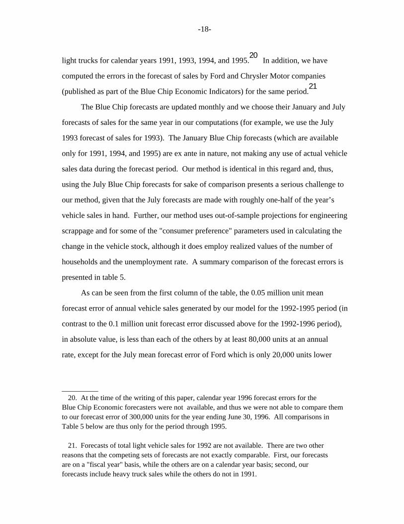
than ours. The second column shows that our forecasts generate root mean squared forecast

errors that are less than one half the size of those associated with the January Blue

Chip, Ford, and Chrysler forecasts; moreover, the root mean squared forecast errors from

Table 5: Forecast Errors: Summary Statistics millions of units)

Sample t-stat F-stat Forecaster Mean RMSE (µ = 0) [MSE(GC)=MSE(i)] (1) (2) (3) (4)

Greenspan/Cohen 0.05 0.29 0.30 n.a.

Blue Chip Consensus Average January -0.13 0.71 -0.26 6.74 July 0.13 0.30 0.84 1.15

Ford Motor Co. January -0.43 0.74 -1.00 5.03 July -0.03 0.24 -0.22 1.44

Chrysler Motor Co. * January -0.77 1.22 -1.16 12.3 July -0.15 0.38 -0.74 1.49 Notes to Table 5: (1) In column 2, RMSE denotes the root mean squared forecast error. (2) Column 3 shows t-statistics for testing the null hypothesis that the mean forecast error is zero, assuming that the mean forecast error is normally distributed. (3) Column 4 shows the F-statistic for testing the null hypothesis that the mean squared forecast error from Greenspan/Cohen (GC) equals the corresponding mean squared error for each of the other three forecasters, assuming that the forecast errors from each of the four forecasters are normally distributed and that the forecast errors are independent across forecasters. * denotes significance at the 10 percent level.

-20-

the July forecasts are all similar in magnitude. Based on this limited evidence, our

forecasts stand up well against others (and perhaps surprisingly well against the July

forecasts).

With only four observations, the results of formal hypothesis testing should be

viewed with some skepticism. Nonetheless, we present the results of two tests, both based

on the assumption that the forecast errors from each method are normally 22 distributed. In column three, we present results of the test of the null hypothesis

that the mean forecast errors are zero (against the alternative that they are not zero);

in all cases, we cannot reject the null hypothesis at conventional significance 23 levels. In column four, we test the null hypothesis of equality of expected squared

forecast errors by use of the variance ratio or F test, under the assumption that the our

forecast errors are independent of the others. The null hypothesis is rejected in the

comparison of Chrysler’s January forecast errors and our own; otherwise it is not 24 rejected.

__________ 22. All small-sample hypothesis tests used here are described in Chapter 11 of Paul Hoel (1962).

23. We also have tested the null hypothesis that the mean forecast error from Greenspan/Cohen equals the corresponding mean error for each of the other three forecasters. The alternative hypothesis is that in absolute value the Greenspan/Cohen mean forecast error is less than that of the other methods. In all cases, we cannot reject the null hypothesis at conventional significance levels.

24. We also have tested the null hypothesis of equality of expected squared forecast errors using an alternative test described in Chapter 9 of C.W.J. Granger and Paul Newbold, (1986). The null hypothesis cannot be rejected in any of the cases examined.

-21-

VI. Conclusion

In this paper, we have offered a new approach to the analysis of motor vehicle sales

in the United States. We have modeled the change in the stock of vehicles in terms of

demographic factors and consumer "preferences." In addition, we have factored vehicle

scrappage into two components. One component reflects physical or "built-in"

deterioration, in which scrappage increases nonlinearly with vehicle age. The other

component incorporates income and relative price effects on the scrappage decision; it is

shown that scrappage varies in a procyclical manner and inversely with the ratio of new

car prices to repair costs. Finally, our approach generates forecasts of aggregate new

vehicle sales which are reasonably accurate and which stand up well in a comparison to

those of the Blue Chip consensus average, Ford Motor Company, and Chrysler Motor Company.

-22-

References

American Automobile Manufacturers Association. AAMA Motor Vehicle Facts and Figures, various issues.

Automotive Recyclers Association, Annual Membership Survey, 1995.

Berkovec, James. "New Car Sales and Used Car Stocks: A Model of the Automobile Market," Rand Journal of Economics, Summer 1985.

Blue Chip Economic Indicators, various issues.

de Wolff, P. "The Demand for Passenger Cars in the United States," Econometrica, April, 1938.

Granger, Clive and Paul Newbold. Forecasting Economic Time Series, 2nd edition, Academic Press, 1986.

Hoel, Paul. Introduction to Mathematical Statistics, 3rd edition, Wiley & Sons, 1962.

Parks, Richard W. "Determinants of Scrapping Rates for Postwar Vintage Automobiles," Econometrica, July 1977, pp. 1099-1115.

. "Durability, Maintenance and the Price of Used Assets, Economic Inquiry, April 1979, pp. 197-217.

Roos, C.F. and Victor Von Szeliski. "Factors Governing Changes in Domestic Automobile Demand," in Dynamics of Automobile Demand, General Motors Corporation, 1939.

Walker, Franklin V. "Determinants of Auto Scrappage," Review of Economics and Statistics, November 1968, pp. 503-506.

Wykoff, Frank C. "Capital Depreciation in the Postwar Period: Automobiles,: Review of Economics and Statistics, 1970, pp. 168-72.

-23-

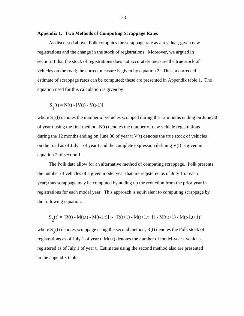
Appendix 1: Two Methods of Computing Scrappage Rates

As discussed above, Polk computes the scrappage rate as a residual, given new

registrations and the change in the stock of registrations. Moreover, we argued in

section II that the stock of registrations does not accurately measure the true stock of

vehicles on the road; the correct measure is given by equation 2. Thus, a corrected

estimate of scrappage rates can be computed; these are presented in Appendix table 1. The

equation used for this calculation is given by:

S (t) = N(t) - [V(t) - V(t-1)] 1

where S (t) denotes the number of vehicles scrapped during the 12 months ending on June 30 1 of year t using the first method; N(t) denotes the number of new vehicle registrations

during the 12 months ending on June 30 of year t; V(t) denotes the true stock of vehicles

on the road as of July 1 of year t and the complete expression defining V(t) is given in

equation 2 of section II.

The Polk data allow for an alternative method of computing scrappage. Polk presents

the number of vehicles of a given model year that are registered as of July 1 of each

year; thus scrappage may be computed by adding up the reduction from the prior year in

registrations for each model year. This approach is equivalent to computing scrappage by

the following equation:

S (t) = [R(t) - M(t,t) - M(t-1,t)] - [R(t+1) - M(t+1,t+1) - M(t,t+1) - M(t-1,t+1)] 2

where S (t) denotes scrappage using the second method; R(t) denotes the Polk stock of 2 registrations as of July 1 of year t; M(t,t) denotes the number of model-year t vehicles

registered as of July 1 of year t. Estimates using the second method also are presented

in the appendix table.

-24-

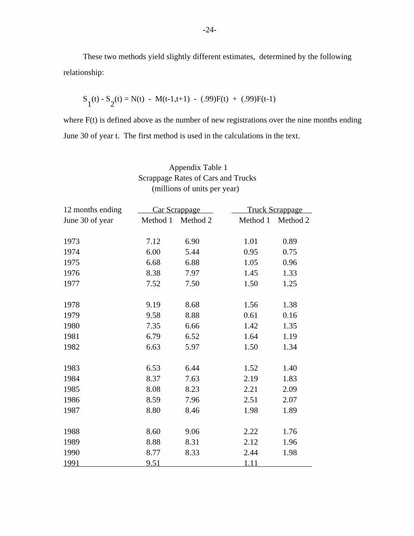
These two methods yield slightly different estimates, determined by the following

relationship:

S (t) - S (t) = N(t) - M(t-1,t+1) - (.99)F(t) + (.99)F(t-1) 1 2

where F(t) is defined above as the number of new registrations over the nine months ending

June 30 of year t. The first method is used in the calculations in the text.

Appendix Table 1 Scrappage Rates of Cars and Trucks (millions of units per year)

12 months ending Car Scrappage Truck Scrappage June 30 of year Method 1 Method 2 Method 1 Method 2

1973 7.12 6.90 1.01 0.89 1974 6.00 5.44 0.95 0.75 1975 6.68 6.88 1.05 0.96 1976 8.38 7.97 1.45 1.33 1977 7.52 7.50 1.50 1.25

1978 9.19 8.68 1.56 1.38 1979 9.58 8.88 0.61 0.16 1980 7.35 6.66 1.42 1.35 1981 6.79 6.52 1.64 1.19 1982 6.63 5.97 1.50 1.34

1983 6.53 6.44 1.52 1.40 1984 8.37 7.63 2.19 1.83 1985 8.08 8.23 2.21 2.09 1986 8.59 7.96 2.51 2.07 1987 8.80 8.46 1.98 1.89

1988 8.60 9.06 2.22 1.76 1989 8.88 8.31 2.12 1.96 1990 8.77 8.33 2.44 1.98 1991 9.51 1.11

-25-

Appendix 2: More on Polk Data and Alternative Data Sources

As mentioned above in section II, the Polk data used in this paper are subject to

the problem of double counting that leads to an overstatement of the number of vehicles in

use. An example of double counting occurs when a resident of Arizona, for example, sells

a used car to a resident of Nevada and the car is simultaneously registered in each state.

Beginning with its July 1993 release, Polk has eliminated double counting of this type

(i.e., interstate) in its 1992 vehicle figures; however, data from prior years have not

been corrected. Owing to processing limitations, Polk does not present the exact amount

of doubling counting but estimates that its population counts may have been inflated by as

much as 1.5 percent (roughly 2.7 million vehicles in 1992) because of interstate

duplication.

Double counting is potentially more of a problem for transfers of car ownership

within a given state. This could happen for cars that are sold used and are registered

twice--once each by the original and new owner--until the original owner does not re-

register the car. In fact, in some states (Oregon and Nevada for example) this is a

problem because the registration, in effect, stays with the owner. However, in other

states, particularly California, the registration stays with the car (i.e., stays with the

vehicle identification number); thus, in California the car sold as used is registered

correctly only once. Polk cuts through differing state treatments by using vehicle

identification numbers to filter the raw registrations or transactions data received from

the states. By comparing the VINs, Polk eliminates all double counting of registrations

within a given state.

In addition to the Polk data, there are several other sources of statistics on the

stock of motor vehicles. The Federal Highway Administration’s annual publication, Highway

Statistics, also presents estimates of total registrations of motor vehicles in the United

States. These estimates always exceed those of Polk; for example, total registrations for

-26-

1990 are 190.3 million as estimated by FHA and 179.3 million as estimated by Polk. The

Polk and FHA data differ for several reasons:

(1) The most fundamental difference is that the Polk estimates give registrations in force at a point in time (July 1st of each year), while the FHA estimates include registrations that have been recorded in state master files at any time during a calendar year. For example, if a car is registered in January, February, and March of a given year, but not registered in April and beyond, it would be counted as a registered car in that year by FHA but not counted at all by Polk. This example best applies to a car that was scrapped during April of the previous year (and thus treated as registered in most states until it was not re-registered in April of the current year).

(2) Another difference, affecting the respective car and truck totals, is that in the FHA approach, autos are defined to include passenger vans and jeeps whereas Polk includes them in the truck totals.

(3) Both FHA and Polk assert that their estimates are mostly purged of double counting of registrations (although Polk claims that FHA data are not purged very well). Elimination of double counting is done by the individual states for FHA, whereas Polk handles the problem internally.

Both Polk and FHA essentially present population totals of the stock of vehicle

registrations in the United States. The Bureau of Economic Analysis produces publicly

available estimates of the end-of-year total stock of motor vehicles as well as separate

estimates of the stock of vehicles used by business and the stock used by households

(computed as a residual from the total, government, and business stocks); these estimates

are derived from several sources, the most important being Polk and Automotive Fleet

magazine. The BEA estimates of the stock of cars and trucks start in 1980 and 1970,

respectively.

The BEA estimates of the total stock of cars are quite similar to the Polk

registrations data; relatively minor differences likely reflect BEA computing stocks as of

the end of the calendar year. However, BEA’s estimates of the stock of trucks are

-27-

substantially less than Polk’s; for example, in 1990 the BEA estimate is about 44 million

and the Polk estimate is about 56 million. The BEA truck estimates are quite similar to

the FHA truck registrations data (even though FHA excludes passenger vans from its

estimates). Moreover, BEA’s estimates of the stock of motor vehicles used by households

are substantially below estimates of other government agencies discussed below (for

example, in 1988 BEA’s estimate of the stock of household vehicles is 135 million,

compared to other estimates of roughly 150 million). This discrepancy may be due in part

to the BEA convention that allocates all "mixed-use" vehicles--i.e., vehicles used both

for business and personal use--to the business stock.

In contrast to the "population" approach of Polk, FHA, and BEA, periodic surveys of

the number of operating vehicles are conducted by the Energy Information Administration

(EIA), Census Bureau, and the Federal Highway Administration; it should be noted that

these surveys provide estimates of the stock of operating vehicles available for household

use only. The EIA’s Residential Transportation Energy Consumption Survey (RTECS) has been

conducted in 1983, 1985, and 1988. The FHA’s Nationwide Personal Transportation Study

(NPTS) has been conducted in 1969, 1977, 1983, and 1990. Census Bureau’s American Housing

Survey (formerly called the Annual Housing Survey) has been conducted in 1970, 1973, 1974,

1975, 1976, 1977, 1980, 1981, 1985, 1987, 1989, 1991, and 1993.

Direct comparison of these three survey estimates is difficult because they differ

with respect to general emphasis, definitions, and implementation; moreover, the three 25 surveys have never been conducted in the same year. However, based on conservative

__________ 25. The NPTS and Census surveys are snapshot or point-in-time estimates of the stock of vehicles kept at home for personal use. Different households are surveyed throughout the sample period (which is September through December for Census). A participant sampled early in the survey period may have a vehicle that is scrapped later in the year, introducing a positive bias into end-of-year estimates. By contrast, the EIA survey avoids such bias by

(Footnote continues on next page)

-28-

assumptions and interpolation methods, it appears that estimates of the stock of household 26 vehicles from the Census and FHA surveys generally exceed those from the EIA survey.

For example, in 1988 the EIA estimate of household vehicles is 147.5 million, compared to

a 155 million estimate based on the Census survey and a 159 million estimate based on the

FHA survey.

The upshot is that the level of the stock of household vehicles differs

substantially across data sources and, at this time, the producers of each data set barely

know of the existence of other estimates, yet alone the reasons for their differences.

Nevertheless, changes in the level over time are quite similar.

__________

(Footnote continued from previous page) sampling a given household three times during the survey year. This makes it possible for a household to have a fraction of a vehicle; for example, if a household owned two vehicles, one for the full year and one for 6 months, that household would be counted as having 1.5 vehicles. NPTS and Census surveys would count this household as having two vehicles, and thus the EIA survey should have a smaller estimate of the aggregate stock of household vehicles (which it does).

26. The FHA and EIA surveys present estimates of the total household stock of vehicles. However, the Census survey presents estimates of the number of households with exactly one, exactly two, and three or more autos available for personal use; for trucks, the number of households with exactly one and two or more are presented. For the sake of calculation, we have used the lower bound of the open-ended categories (i.e., 3 for autos and 2 for trucks).

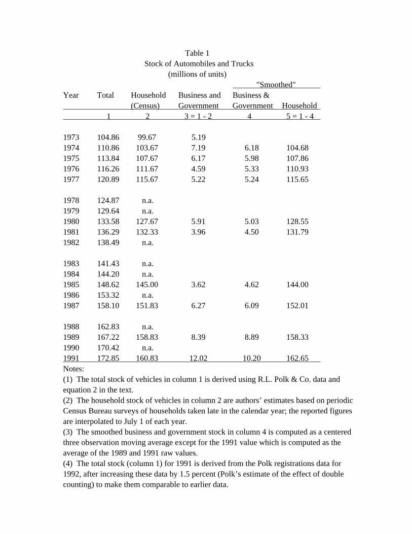
Table 1 Stock of Automobiles and Trucks (millions of units) "Smoothed" Year Total Household Business and Business & (Census) Government Government Household 1 2 3 = 1 - 2 4 5 = 1 - 4

1973 104.86 99.67 5.19 1974 110.86 103.67 7.19 6.18 104.68 1975 113.84 107.67 6.17 5.98 107.86 1976 116.26 111.67 4.59 5.33 110.93 1977 120.89 115.67 5.22 5.24 115.65

1978 124.87 n.a. 1979 129.64 n.a. 1980 133.58 127.67 5.91 5.03 128.55 1981 136.29 132.33 3.96 4.50 131.79 1982 138.49 n.a.

1983 141.43 n.a. 1984 144.20 n.a. 1985 148.62 145.00 3.62 4.62 144.00 1986 153.32 n.a. 1987 158.10 151.83 6.27 6.09 152.01

1988 162.83 n.a. 1989 167.22 158.83 8.39 8.89 158.33 1990 170.42 n.a. 1991 172.85 160.83 12.02 10.20 162.65 Notes: (1) The total stock of vehicles in column 1 is derived using R.L. Polk & Co. data and equation 2 in the text. (2) The household stock of vehicles in column 2 are authors’ estimates based on periodic Census Bureau surveys of households taken late in the calendar year; the reported figures are interpolated to July 1 of each year. (3) The smoothed business and government stock in column 4 is computed as a centered three observation moving average except for the 1991 value which is computed as the average of the 1989 and 1991 raw values. (4) The total stock (column 1) for 1991 is derived from the Polk registrations data for 1992, after increasing these data by 1.5 percent (Polk’s estimate of the effect of double counting) to make them comparable to earlier data.

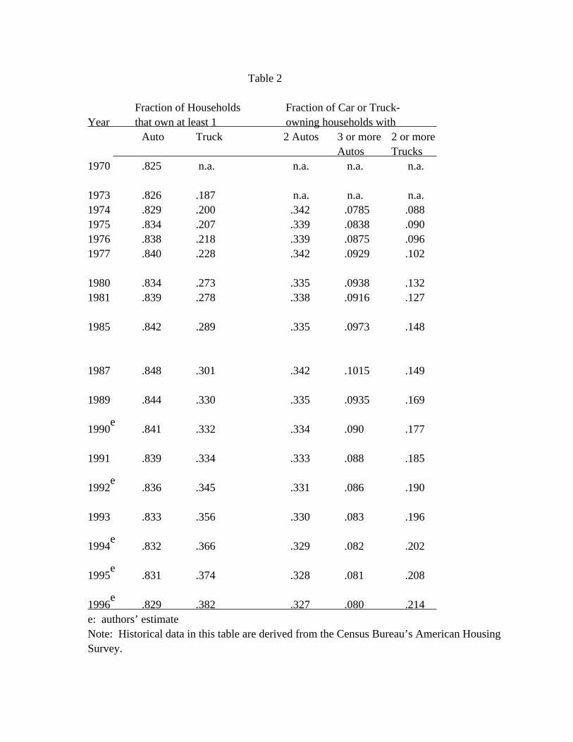
Table 2

Fraction of Households Fraction of Car or Truck- Year that own at least 1 owning households with Auto Truck 2 Autos 3 or more 2 or more Autos Trucks 1970 .825 n.a. n.a. n.a. n.a.

1973 .826 .187 n.a. n.a. n.a. 1974 .829 .200 .342 .0785 .088 1975 .834 .207 .339 .0838 .090 1976 .838 .218 .339 .0875 .096 1977 .840 .228 .342 .0929 .102

1980 .834 .273 .335 .0938 .132 1981 .839 .278 .338 .0916 .127

1985 .842 .289 .335 .0973 .148

1987 .848 .301 .342 .1015 .149

1989 .844 .330 .335 .0935 .169

e 1990 .841 .332 .334 .090 .177

1991 .839 .334 .333 .088 .185

e 1992 .836 .345 .331 .086 .190

1993 .833 .356 .330 .083 .196

e 1994 .832 .366 .329 .082 .202

e 1995 .831 .374 .328 .081 .208

e 1996 .829 .382 .327 .080 .214 e: authors’ estimate Note: Historical data in this table are derived from the Census Bureau’s American Housing Survey.

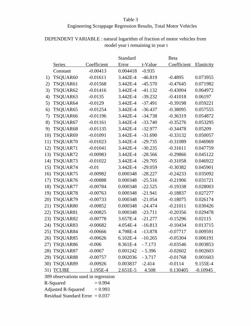
Table 3 Engineering Scrappage Regression Results, Total Motor Vehicles

DEPENDENT VARIABLE : natural logarithm of fraction of motor vehicles from model year i remaining in year t

Standard Beta Series Coefficient Error t-Value Coefficient Elasticity Constant -0.00413 0.004418 -0.935 1) TSQUAR60 -0.01611 3.442E-4 -46.819 -0.4895 0.073955 2) TSQUAR61 -0.01568 3.442E-4 -45.570 -0.47645 0.071982 3) TSQUAR62 -0.01416 3.442E-4 -41.132 -0.43004 0.064972 4) TSQUAR63 -0.0135 3.442E-4 -39.232 -0.41018 0.06197 5) TSQUAR64 -0.0129 3.442E-4 -37.491 -0.39198 0.059221 6) TSQUAR65 -0.01254 3.442E-4 -36.437 -0.38095 0.057555 7) TSQUAR66 -0.01196 3.442E-4 -34.738 -0.36319 0.054872 8) TSQUAR67 -0.01161 3.442E-4 -33.740 -0.35276 0.053295 9) TSQUAR68 -0.01135 3.442E-4 -32.977 -0.34478 0.05209 10) TSQUAR69 -0.01091 3.442E-4 -31.690 -0.33132 0.050057 11) TSQUAR70 -0.01023 3.442E-4 -29.735 -0.31089 0.046969 12) TSQUAR71 -0.01041 3.442E-4 -30.235 -0.31611 0.047759 13) TSQUAR72 -0.00983 3.442E-4 -28.566 -0.29866 0.045122 14) TSQUAR73 -0.01022 3.442E-4 -29.705 -0.31058 0.046922 15) TSQUAR74 -0.01 3.442E-4 -29.059 -0.30382 0.045901 16) TSQUAR75 -0.00982 0.000348 -28.227 -0.24233 0.035092 17) TSQUAR76 -0.00888 0.000348 -25.516 -0.21906 0.031721 18) TSQUAR77 -0.00784 0.000348 -22.525 -0.19338 0.028003 19) TSQUAR78 -0.00763 0.000348 -21.941 -0.18837 0.027277 20) TSQUAR79 -0.00733 0.000348 -21.054 -0.18075 0.026174 21) TSQUAR80 -0.00852 0.000348 -24.474 -0.21011 0.030426 22) TSQUAR81 -0.00825 0.000348 -23.711 -0.20356 0.029478 23) TSQUAR82 -0.00778 3.657E-4 -21.277 -0.15296 0.02115 24) TSQUAR83 -0.00682 4.054E-4 -16.813 -0.10434 0.013715 25) TSQUAR84 -0.00666 4.798E-4 -13.878 -0.07717 0.009591 26) TSQUAR85 -0.00626 6.102E-4 -10.265 -0.05304 0.006191 27) TSQUAR86 -0.006 8.361E-4 - 7.173 -0.03546 0.003853 28) TSQUAR87 -0.0067 0.001242 - 5.396 -0.02602 0.002603 29) TSQUAR88 -0.00757 0.002036 - 3.717 -0.01768 0.001603 30) TSQUAR89 -0.00926 0.003837 -2.414 -0.0114 9.155E-4 31) TCUBE 1.195E-4 2.651E-5 4.508 0.130405 -0.10945 309 observations used in regression R-Squared = 0.994 Adjusted R-Squared = 0.993 Residual Standard Error = 0.037

10

20

30

40

50

60

70

80

90

10

0

11

0

12

34

56

78

91

01

11

21

31

41

5

19

60

Mo

de

l

19

65

Mo

de

l

19

70

Mo

de

l

19

80

Mo

de

l

19

86

Mo

de

l

19

88

Mo

de

l

Ye

ars

Afte

r M

od

el In

tro

du

ce

d

19

60

Mo

de

l Y

ea

r1

96

5 M

od

el Y

ea

r1

97

0 M

od

el Y

ea

r1

98

0 M

od

el Y

ea

r1

98

6 M

od

el Y

ea

r1

98

8 M

od

el Y

ea

r

Ch

art

1.

Pe

rce

nt

of

To

tal M

oto

r V

eh

icle

s R

em

ain

ing

in

Use

Pe

rce

nt R

em

ain

ing

19

73

19

75

19

77

1979

1981

1983

1985

1987

1989

1991

2.5

21.5

10.5

0 –+0.5

11.5

22.5

Ch

art

2:

Cy

cli

ca

l S

cra

pp

ag

e,

To

tal

Mo

tor

Ve

hic

les

Mill

ions

of

vehic

les