Motion of spinning test bodies in Kerr spacetime

Eva Hackmann,1,* Claus Lämmerzahl,1,2,† Yuri N. Obukhov,3,‡ Dirk Puetzfeld,1,§ and Isabell Schaffer1,2,∥1ZARM, University of Bremen, Am Fallturm, 28359 Bremen, Germany2Institut für Physik, Universität Oldenburg, 26111 Oldenburg, Germany

3Theoretical Physics Laboratory, Nuclear Safety Institute, Russian Academy of Sciences,B.Tulskaya 52, 115191 Moscow, Russia

(Received 8 August 2014; published 22 September 2014)

We investigate the motion of spinning test bodies in General Relativity. By means of a multipolarapproximation method for extended test bodies we derive the equations of motion and classify the orbitalmotion of pole-dipole test bodies in the equatorial plane of the Kerr geometry. An exact expression for theperiastron shift of a spinning test body is given. Implications of test body spin corrections are studied andcompared with the results obtained by means of other approximation schemes.

DOI: 10.1103/PhysRevD.90.064035 PACS numbers: 04.25.-g, 04.20.-q

I. INTRODUCTION

Extreme mass ratios in astrophysical situations, forexample as found in the Galactic center, allow for anapproximate analytic description of the motion in certainparameter regimes. The steadily improving observationalsituation of the Galactic center [1–3] may soon enable us totest different competing theoretical approaches to modelthe motion of astrophysical objects in the theory of GeneralRelativity.In this work we study the motion of extended spinning

test bodies in a Kerr background. Our starting point is anexplicit velocity formula based on the multipolar descrip-tion [4–8] of pole-dipole test bodies, with the help of whichwe classify the orbital motion in the equatorial plane of aKerr black hole for aligned and anti-aligned test body spin.An exact expression for the periastron shift is given andcompared with corresponding post-Newtonian results. Weprovide an estimate of the test body spin corrections fororbits around the black hole in the Galactic center.The structure of the paper is as follows. In Sec. II we

provide the equations of motion for spinning test bodiesand derive a general formula which relates the momentumand the velocity of the test body. The motion of spinningtest bodies is then studied in a Kerr background in Sec. III.These equations of motion are of a mathematical structurewhich allows for an analytic solution [9,10] and a system-atic classification of different orbit types in Sec. IV. InSec. Va general formula for the periastron shift is given andcompared to corresponding post-Newtonian results. Ourconclusions are drawn in Sec. VI. In Appendixes A and Bwe provide some supplementary material and a summary ofour conventions.

II. EQUATIONS OF MOTION OFSPINNING TEST BODIES

The equations of motion of spinning extended test bodiesup to the pole-dipole order have been derived in severalworks [4–8,11] by means of different multipolar approxi-mation techniques and are given by the following set ofequations:

Dpa

ds¼ 1

2RabcdubScd; ð1Þ

DSab

ds¼ 2p½aub�: ð2Þ

Here ua ≔ dYa=ds denotes the 4-velocity of the bodyalong its world line (normalized to uaua ¼ 1), pa themomentum, Sab ¼ −Sba the spin, D

ds the covariant deriva-tive along ua, and Rabcd is the Riemannian curvature.Equation (2) implies that the momentum is given by

pa ¼ mua þDSab

dsub; ð3Þ

where m ≔ paua. Note that in order to close the system ofequations (1)–(2) a supplementary condition has to beimposed.

A. Conserved quantities

If ξa is a Killing vector, i.e.∇ðbξaÞ ¼ 0, then the quantity,

Eξ ¼ paξa þ 1

2Sab∇aξb; ð4Þ

is conserved (see e.g. [11,12] for a derivation).Other conserved quantities depend on the supplementary

condition. In the pole-dipole case, the spin length Sgiven by

*eva.hackmann@zarm.uni‑bremen.de†claus.laemmerzahl@zarm.uni‑bremen.de‡obukhov@ibrae.ac.ru§dirk.puetzfeld@zarm.uni‑bremen.de; http://puetzfeld.org∥trisax@t‑online.de

PHYSICAL REVIEW D 90, 064035 (2014)

1550-7998=2014=90(6)=064035(12) 064035-1 © 2014 American Physical Society

S2 ≔1

2SabSab ð5Þ

is conserved for the two well-known supplementaryconditions of Tulczyjew,

paSab ¼ 0; ð6Þ

and Frenkel,

uaSab ¼ 0: ð7Þ

Apart from m one may define a mass m by m2 ≔ papa.In the pole-dipole case m is conserved if one choosesTulczyjew’s spin supplementary condition (6). However,for the Frenkel condition (7) the massm is conserved in thepole-dipole case.

B. Velocity-momentum relation

For either of the two supplementary conditions (6) or (7)the following relation, see [13] for a derivation, between thevelocity and the momentum holds,

ua ¼ð6Þ∨ð7Þpa þ 2SacSdeRdecb

4m2 þ ScdSefRcdefpb; ð8Þ

where

pa ≔mm2

pa −1

m2

Dds

ðSabpbÞ: ð9Þ

From the velocity formula (8) and the normalizationcondition uaua ¼ 1, we obtain—for the Tulczyjewcondition—(6) an explicit expression for the mass m ofthe following form,

m ¼ð6Þ m2

μ; ð10Þ

where we introduced auxiliary quantities,

μ2 ¼ m2 þ A21S

abScdRcdbepeSafSghRghfipi; ð11Þ

A1 ¼2

4m2 þ SabScdRcdab: ð12Þ

In flat spacetime we have m ¼ μ ¼ m. Resubstituting (10)back into (8), we obtain an expression for the velocity,

ua ¼ð6ÞKabpb; ð13Þ

Kab ¼

1

μðδab − A1SaeScdRbecdÞ; ð14Þ

as a function of the momentum, the mass m, and the spin,i.e. ua ¼ uaðm;pa; Sab; RabcdÞ.

C. Nonlinear dynamics of spin

For the Tulczyjew condition (6) we define the spin vectorSa as

Sa ≔1

2mffiffiffiffiffiffi−gp εabcdpbScd;

Sab ¼ 1

mffiffiffiffiffiffi−gp εabcdpcSd: ð15Þ

Here εabcd is the totally antisymmetric Levi-Civita symbol;the only nontrivial component is equal ε0123 ¼ 1. It isstraightforward to derive the equation of motion for thevector of spin:

DSa

ds¼ papb

m2

DSb

ds: ð16Þ

By construction, we have the orthogonality

paSa ¼ 0; ð17Þ

and noticing that SabSb ¼ 0 from (15), we use (13) and (14)to verify another orthogonality property,

uaSa ¼ 0: ð18Þ

Substituting the velocity-momentum relation (13) and (14)into (1) and (16), we derive the closed system of dynamicalequations for the momentum and spin vectors,

Dpa

ds¼ 1

2Ke

aRebcdpbScd; ð19Þ

DSa

ds¼ −

papb

2m2Ke

fRebcdScdSf: ð20Þ

Contracting (16) or (20) with Sa, we verify that the lengthof the spin vector is constant by making use of (17). From(15) we find

SaSa ¼ −1

2SabSab ¼ −S2; ð21Þ

where we recall the definition of the spin length (5). Thevector of spin is therefore spacelike.The dynamical equations (19) and (20) are highly

nonlinear in spin. Indeed, the right-hand sides of theseequations contain

EVA HACKMANN et al. PHYSICAL REVIEW D 90, 064035 (2014)

064035-2

Kab ¼

1

μ

�δab − 2A1

�δac −

papc

m2

�ðS2δcd þ ScSdÞ

×

�Rd

b þ Rdkbn

�pkpn

m2−SkSn

S2

���: ð22Þ

Furthermore, we explicitly have

μ2 ¼ m2 þ 4A21½S2ðRabpaSbÞ2

−1

m2ðS2Rabpapb − RacbdpapbScSdÞ2

þ ðS2Rab − RaebfSeSfÞpbðS2Rac − RakcnSkSnÞpc�;ð23Þ

1

A1

¼ 2½m2 − RacbdSaSbpcpd=m2

− RabðSaSb þ gabS2=2þ papb=m2Þ�: ð24Þ

Here Rab is the Ricci tensor.The analysis of the nonlinear system (19) and (20) is a

complicated problem, in general. A perturbation schemewas developed in [14–17] to deal with the full nonlinearsystem. In this approach, one linearizes the equations ofmotion to obtain

Dpa

ds≈

1

2RabcdpbScd; ð25Þ

DSa

ds≈ 0; ð26Þ

and the solution of the full system is then constructed as aseries in the powers of spin S, which is used as aperturbation parameter. In the linearized case, we againhave m ¼ μ ¼ m and hence pa ≈ mua. It is worthwhile tonote that the Gravity Probe B experiment [18,19] is actuallybased on the linearized equations of motion (25) and (26).In this paper, we analyze the complete nonlinear equa-

tions of motion without using approximations and pertur-bation theory.

III. EQUATIONS OF MOTION IN A KERRBACKGROUND

In the following, we are going to study test bodiesendowed with spin in the gravitational field of a rotatingsource described by the Kerr metric. This problem wasinvestigated in the past for the Tulczyjew supplementarycondition (see [17,20], e.g.), as well as for the Frenkelcondition [21,22]. In view of the complexity of theproblem, the solution in most cases was obtained numeri-cally and/or approximately with the help of perturbationtheory.Here we will specialize to the integrable case for which

we obtain an exact and analytical result. The full nonlinear

equations of motion are considered, no linearizationor other approximation is made. Since the Kerr metricsatisfies the vacuum Einstein field equation, Rab ¼ 0, theformulas (22)–(24) become significantly simpler.

A. The Kerr metric

In Boyer-Lindquist coordinates ðt; r; θ;ϕÞ, the Kerrmetric takes the form

ds2 ¼�1−

2Mrρ2

�dt2þ 4aMrsin2θ

ρ2dtdϕ−

ρ2

Δdr2

− ρ2dθ2− sin2θ

�r2þa2þ 2a2Mrsin2θ

ρ2

�dϕ2; ð27Þ

where M is the mass parameter, a the Kerr parameter, and

Δ ≔ r2 − 2Mrþ a2; ð28Þ

ρ2 ≔ r2 þ a2cos2θ: ð29Þ

The Kerr metric allows for two Killing vector fields givenby

ξaE¼ δat ; ξa

J¼ δaϕ: ð30Þ

Furthermore, we have

ffiffiffiffiffiffi−g

p≔

ffiffiffiffiffiffiffiffiffiffiffiffiffiffiffiffiffiffiffiffi− detðgabÞ

p¼ ρ2 sin θ: ð31Þ

B. Equatorial orbits for polar spin

Let us assume that the spin vector of a test body has onlyone, namely polar, component:

Sa ¼ Sθδaθ : ð32Þ

In view of the orthogonality relations (17) and (18) thepolar ansatz (32) yields

pθ ¼ 0; uθ ¼ 0: ð33Þ

Recalling uθ ¼ dθ=ds, we thus conclude that the polarangle is fixed, θ ¼ const. Therefore, we can focus onequatorial orbits, i.e.

θ ¼ π

2: ð34Þ

The consistency of the equatorial setup (32)–(34) wasanalyzed earlier in [23]. It is worthwhile to note that theassumption (32) on the equatorial plane means that the spinof a test body is aligned with the spin of the Kerr source.Let us now turn to the integration of the equations of

motion (19) and (20). The polar ansatz (32) and its

MOTION OF SPINNING TEST BODIES IN KERR SPACETIME PHYSICAL REVIEW D 90, 064035 (2014)

064035-3

corollary (33) leave us with the four unknownsfpt; pr; pϕ; Sθg, which should be determined from theequations of motion. Fortunately, we have exactly fourintegrals of motion and we can find the nontrivial compo-nents of the vectors of momentum and spin from thefollowing set of equations,

S2 ¼ −SaSa; ð35Þ

m2 ¼ papa; ð36Þ

E ¼ pa

�ξaEþ εabcd

2mffiffiffiffiffiffi−gp Sb∇cξd

E

�; ð37Þ

−J ¼ pa

�ξaJþ εabcd

2mffiffiffiffiffiffi−gp Sb∇cξd

J

�; ð38Þ

in terms of the mass m, the spin length S, the energy E, andthe angular momentum J.From the length conservation of spin (35), we immedi-

ately find Sθ ¼ S=ffiffiffiffiffiffiffiffiffiffi−gθθ

p. For completeness we can use

(15) to write down the nontrivial components of the spintensor in the equatorial plane:

Srt ¼ −Spϕ

mr; Sϕt ¼ Spr

mr; Sϕr ¼ −

Spt

mr: ð39Þ

The algebraic system (37) and (38) can be solved for themomentum components pt and pϕ in terms of the constantsof motion:

pt ¼E − MS

mr3 ðJ − aEÞ1 − MS2

m2r3; ð40Þ

pϕ ¼−J − aMS

mr3 ½aEð1 − r3

a2MÞ − J�1 − MS2

m2r3: ð41Þ

The remaining component pr is obtained from (36).

C. Orbital equation of motion

With the help of (13), (22)–(24), (40), and (41) we canderive explicit expressions for the velocity components interms of the constants of motion and the parameters of thetest body, i.e. ua ¼ uaðm; S; E; J; a;MÞ. From this wederive an explicit expression for ur=uϕ,

drdϕ

¼ Δðr3 þ S2Þr Q

ffiffiffiffiffiffiPa

q; ð42Þ

where we introduced the dimensionless quantities,

r ¼ rM

; a ¼ aM

; J ¼ JmM

;

E ¼ Em; S ¼ S

mM; ð43Þ

and

Pa¼ðE2−1Þr8þ2r7þða2ðE2−1Þ−ðSE−JÞ2Þr6þ2ððSE−JÞ2þ SðS−EJÞþ aEðaEþ3SE−2JÞÞr5−4S2r4þ2aSðJ2−ESJþa2E2þE2Sa−2aJ EþSaÞr3þ S2ððaE−JÞ2− S2Þr2þ2S4r− a2S4; ð44Þ

Q¼ðJ− SEÞr6þðSE þ aE−JÞð2r5þ Sðaþ2SÞr3−4S2r2þ3a2S2rÞþ S3aðaE−JÞ; ð45Þ

with Δ ¼ r2 − 2rþ a2. In the following all quantities witha bar are always dimensionless.

D. Integration

The equation of motion (42) can be integrated analyti-cally in a parametric form. First we notice that thecorresponding integral equation,

ϕ − ϕ0 ¼Z

r

r0

r Q

ΔðS2 þ r3ÞffiffiffiffiffiffiPa

p dr; ð46Þ

contains on the right-hand side a hyperelliptic integral ofgenus three and the third kind. The corresponding problemfor genus two was recently solved analytically [24] in aparametric form by introducing a new affine parameter λ,which may be considered as an analogue of the Mino time[25]. Together with the analytic solution of integralequations involving hyperelliptic integrals of genus threeand the first kind [9], the solution rðλÞ and ϕðλÞ can befound analytically. However, we will not elaborate this herebut rather focus on the related classification of the orbits,and on the periastron shift in Sec. V.

IV. CLASSIFICATION OF ORBITAL MOTION

Wewill now analyze the orbital motion in the consideredsetting of equatorial motion with aligned spin. Observe thatthe substitutions ða; J; SÞ → ð−a;−J;−SÞ and ðE; JÞ →ð−E;−JÞ only change the sign of the equation of motion,drdϕ → − dr

dϕ. Therefore, this only reverses the direction butleaves the type of orbit unchanged, so we choose a ≥ 0

and E ≥ 0.

EVA HACKMANN et al. PHYSICAL REVIEW D 90, 064035 (2014)

064035-4

A. Circular motion

From Eq. (42) it can be inferred that the expression underthe square root given by (44) has to be positive to getphysical meaningful results. Only if Pa ≥ 0 motion ispossible for the given parameters of the spacetime andthe particle. The points Pa ¼ 0 define the turning points of

the motion. Coinciding turning points correspond tocircular orbits and are given by double zeros of Pa,

Pa ¼ 0;dPa

dr¼ 0: ð47Þ

Solving this two conditions for E and J yields

E1;2;3;4 ¼ �ffiffiffir

pffiffiffi2

pr3Va

fVaðRa � Δ½U2að9a2S4 þ 6Sr2ðS2 þ 2r3Þaþ rð4r6 þ 13r3S2 − 8S4ÞÞ�12Þg1

2; ð48Þ

J1;2;3;4 ¼1

r3EUafð3rS5 þ 3r7ð2E2 − 1ÞSÞa3 þ ðS6 þ r3ðE2 − 3rþ 6ÞS4 þ 3r6ðrE2 þ r − 2þ 4E2ÞS2

þ r9ð2E2 − 1ÞÞa2 þ ðr2ðr − 4ÞS5 − r5ð3r2E2 − 9E2 − 4r − 4rE2 þ 4ÞS3 þ r8ð8rE2 − 5rþ 8ÞSÞa − rS6

− r4ð2r − 3Þðrþ rE2 − 4ÞS4 þ r7ðr2 þ 9 − 7rþ 3rE2ÞS2 − r10ð−3rE2 þ r2E2 þ 4r − 4 − r2Þg; ð49Þ

where

Va ¼ −6S rðS2 þ 2r3ÞΔ aþðð3r − 4ÞS4 þ r3ð6r − 19ÞS2 − 4r6Þa2 þ rð2r − 3Þ2S4 þ r4ð4r2 − 27rþ 36ÞS2 þ r7ðr − 3Þ2;ð50Þ

Ra ¼ −18S3a5r4 þ ð3S6 þ 3ð3r − 4Þr3S4 þ 18S2r6Þa4 þ ð8r2S5 − 2r5ð27r − 67ÞS3 − 2r8ð9r − 19ÞSÞa3þ ð5rðr − 2ÞS6 þ r4ð15r2 þ 87 − 70rÞS4 þ r7ð12r2 þ 30 − 37rÞS2 − 2r10ð3r − 5ÞÞa2− ð4r3ðr2 þ 5 − 4rÞS5 þ 2r6ð−77rþ 14r2 þ 94ÞS3 þ 2r9ð11r2 − 41rþ 40ÞSÞaþ 2r2ð3 − 2rÞS6 þ ð8r3 − 56r2 þ 145r − 126Þr5S4 þ ð8r3 − 65r2 þ 160r − 126Þr8S2 þ 2r11ðr − 3Þðr − 2Þ2; ð51Þ

Ua ¼ 6Sr4a2 þ ðS4 þ 12r3S2 − 3r4S2 þ 2r6Þa − Sr2ð4S2r − r4 − 9S2Þ: ð52Þ

If in addition to the conditions (47) also d2Padr2 < 0 holds,

then the circular orbit is stable against radial perturbations.The radius of the innermost stable circular orbit (ISCO)

with d2Padr2 ¼ 0 is of particular importance as it marks the

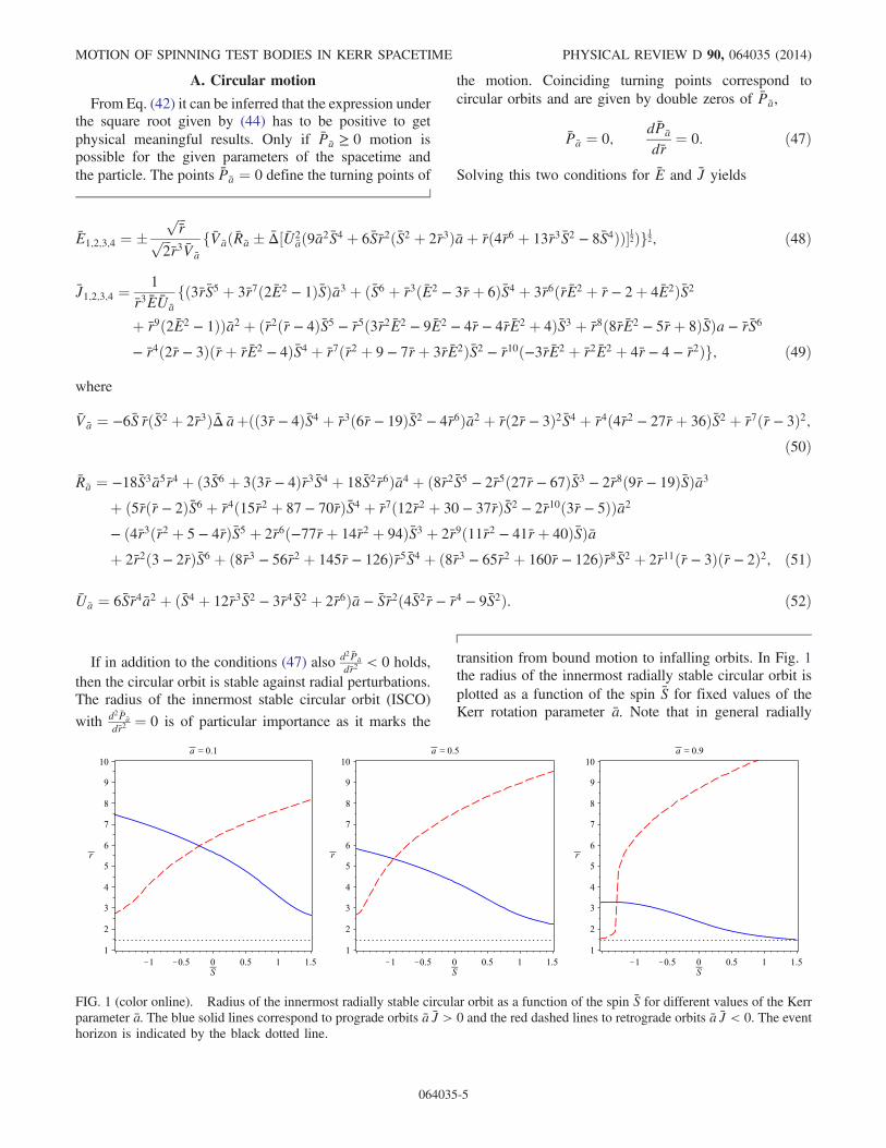
transition from bound motion to infalling orbits. In Fig. 1the radius of the innermost radially stable circular orbit isplotted as a function of the spin S for fixed values of theKerr rotation parameter a. Note that in general radially

FIG. 1 (color online). Radius of the innermost radially stable circular orbit as a function of the spin S for different values of the Kerrparameter a. The blue solid lines correspond to prograde orbits a J > 0 and the red dashed lines to retrograde orbits a J < 0. The eventhorizon is indicated by the black dotted line.

MOTION OF SPINNING TEST BODIES IN KERR SPACETIME PHYSICAL REVIEW D 90, 064035 (2014)

064035-5

stable orbits may still be unstable against perturbations inthe θ-direction. Suzuki and Maeda [26] have shown thatradially stable circular orbits become unstable in the θdirection for large positive spin values S ≳ 0.9, but theyonly considered prograde motion (a J > 0). However, fromFig. 1 we infer that radially stable retrograde circular orbitswith negative spins may come closer to the horizon than thecorresponding prograde orbits (see also [27]). Therefore, itwould be interesting to analyze whether the same insta-bilities as reported in [26] also appear for retrograde orbitswith negative spins.

B. General orbits

For given values of the parameters of the spacetime andthe particle all possible types of motion are given by theregions where Pa ≥ 0, which can be directly inferred fromthe number of turning points Pa ¼ 0 and the asymptoticbehaviour of Pa at infinity. If we continuously vary thevalues of the parameters, the number of turning pointschanges at that set of parameters which correspond to

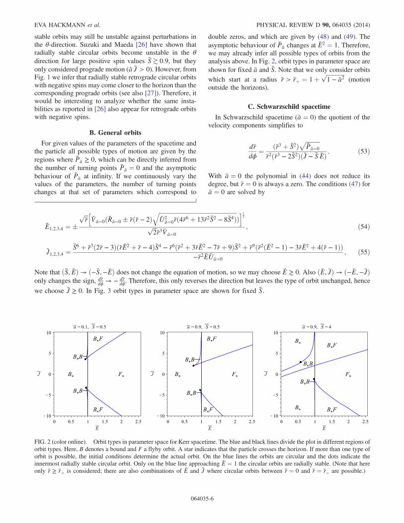
double zeros, and which are given by (48) and (49). Theasymptotic behaviour of Pa changes at E2 ¼ 1. Therefore,we may already infer all possible types of orbits from theanalysis above. In Fig. 2, orbit types in parameter space areshown for fixed a and S. Note that we only consider orbitswhich start at a radius r > rþ ¼ 1þ

ffiffiffiffiffiffiffiffiffiffiffiffiffi1 − a2

p(motion

outside the horizons).

C. Schwarzschild spacetime

In Schwarzschild spacetime (a ¼ 0) the quotient of thevelocity components simplifies to

drdϕ

¼ ðr3 þ S2ÞffiffiffiffiffiffiffiffiffiffiPa¼0

pr2ðr3 − 2S2ÞðJ − S EÞ : ð53Þ

With a ¼ 0 the polynomial in (44) does not reduce itsdegree, but r ¼ 0 is always a zero. The conditions (47) fora ¼ 0 are solved by

E1;2;3;4 ¼ �ffiffiffir

p hVa¼0ðRa¼0 � rðr − 2Þ

ffiffiffiffiffiffiffiffiffiffiffiffiffiffiffiffiffiffiffiffiffiffiffiffiffiffiffiffiffiffiffiffiffiffiffiffiffiffiffiffiffiffiffiffiffiffiffiffiffiffiffiffiffiffiU2

a¼0rð4r6 þ 13r2S2 − 8S4Þq

Þi12

ffiffiffi2

pr3Va¼0

; ð54Þ

J1;2;3;4 ¼S6 þ r3ð2r − 3ÞðrE2 þ r − 4ÞS4 − r6ðr2 þ 3rE2 − 7rþ 9ÞS2 þ r9ðr2ðE2 − 1Þ − 3rE2 þ 4ðr − 1ÞÞ

−r2EUa¼0

; ð55Þ

Note that ðS; EÞ → ð−S;−EÞ does not change the equation of motion, so we may choose E ≥ 0. Also ðE; JÞ → ð−E;−JÞonly changes the sign, dr

dϕ → − drdϕ. Therefore, this only reverses the direction but leaves the type of orbit unchanged, hence

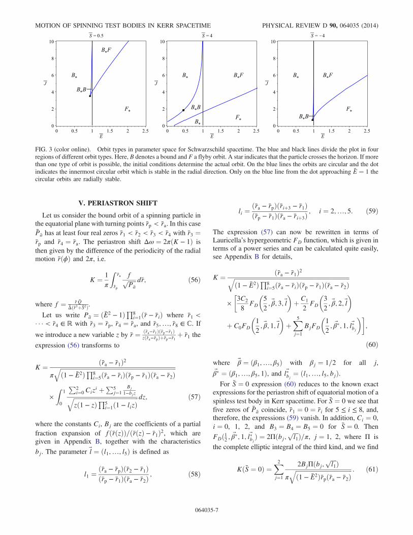
we choose J ≥ 0. In Fig. 3 orbit types in parameter space are shown for fixed S.

FIG. 2 (color online). Orbit types in parameter space for Kerr spacetime. The blue and black lines divide the plot in different regions oforbit types. Here, B denotes a bound and F a flyby orbit. A star indicates that the particle crosses the horizon. If more than one type oforbit is possible, the initial conditions determine the actual orbit. On the blue lines the orbits are circular and the dots indicate theinnermost radially stable circular orbit. Only on the blue line approaching E ¼ 1 the circular orbits are radially stable. (Note that hereonly r ≥ rþ is considered; there are also combinations of E and J where circular orbits between r ¼ 0 and r ¼ r− are possible.)

EVA HACKMANN et al. PHYSICAL REVIEW D 90, 064035 (2014)

064035-6

V. PERIASTRON SHIFT

Let us consider the bound orbit of a spinning particle inthe equatorial plane with turning points rp < ra. In this casePa has at least four real zeros r1 < r2 < r3 < r4 with r3 ¼rp and r4 ¼ ra. The periastron shift Δω ¼ 2πðK − 1Þ isthen given by the difference of the periodicity of the radialmotion rðϕÞ and 2π, i.e.

K ¼ 1

π

Zra

rp

fffiffiffiffiffiffiPa

p dr; ð56Þ

where f ¼ r QΔðr3þS2Þ.

Let us write Pa ¼ ðE2 − 1ÞQ8i¼1ðr − riÞ where r1 <

� � � < r4 ∈ R with r3 ¼ rp, r4 ¼ ra, and r5;…; r8 ∈ C. If

we introduce a new variable z by r ¼ ðra−r1Þðrp−r1Þzðra−rpÞþrp−r1

þ r1 the

expression (56) transforms to

K ¼ ðra − r1Þ2π

ffiffiffiffiffiffiffiffiffiffiffiffiffiffiffiffiffiffiffiffiffiffiffiffiffiffiffiffiffiffiffiffiffiffiffiffiffiffiffiffiffiffiffiffiffiffiffiffiffiffiffiffiffiffiffiffiffiffiffiffiffiffiffiffiffiffiffiffiffiffiffiffiffiffiffiffiffiffið1 − E2ÞQ8

i¼5ðra − riÞðrp − r1Þðra − r2Þq

×Z

1

0

P2i¼0 Cizi þ

P5j¼1

Bj

1−bjzffiffiffiffiffiffiffiffiffiffiffiffiffiffiffiffiffiffiffiffiffiffiffiffiffiffiffiffiffiffiffiffiffiffiffiffiffiffiffiffiffiffiffiffizð1 − zÞQ5

i¼1ð1 − lizÞq dz; ð57Þ

where the constants Ci, Bj are the coefficients of a partialfraction expansion of fðrðzÞÞ=ðrðzÞ − r1Þ2, which aregiven in Appendix B, together with the characteristics

bj. The parameter ~l ¼ ðl1;…; l5Þ is defined as

l1 ¼ðra − rpÞðr2 − r1Þðrp − r1Þðra − r2Þ

; ð58Þ

li ¼ðra − rpÞðriþ3 − r1Þðrp − r1Þðra − riþ3Þ

; i ¼ 2;…; 5: ð59Þ

The expression (57) can now be rewritten in terms ofLauricella’s hypergeometric FD function, which is given interms of a power series and can be calculated quite easily,see Appendix B for details,

K ¼ ðra − r1Þ2ffiffiffiffiffiffiffiffiffiffiffiffiffiffiffiffiffiffiffiffiffiffiffiffiffiffiffiffiffiffiffiffiffiffiffiffiffiffiffiffiffiffiffiffiffiffiffiffiffiffiffiffiffiffiffiffiffiffiffiffiffiffiffiffiffiffiffiffiffiffiffiffiffiffiffiffiffiffið1 − E2ÞQ8

i¼5ðra − riÞðrp − r1Þðra − r2Þq

×

�3C2

8FD

�5

2; ~β; 3;~l

�þ C1

2FD

�3

2; ~β; 2;~l

�

þ C0FD

�1

2; ~β; 1;~l

�þX5j¼1

BjFD

�1

2; ~β�; 1; ~l�bj

��;

ð60Þ

where ~β ¼ ðβ1;…; β5Þ with βj ¼ 1=2 for all j,~β� ¼ ðβ1;…; β5; 1Þ, and ~l�bj ¼ ðl1;…; l5; bjÞ.For S ¼ 0 expression (60) reduces to the known exact

expressions for the periastron shift of equatorial motion of aspinless test body in Kerr spacetime. For S ¼ 0 we see thatfive zeros of Pa coincide, r1 ¼ 0 ¼ ri for 5 ≤ i ≤ 8, and,therefore, the expressions (59) vanish. In addition, Ci ¼ 0,i ¼ 0, 1, 2, and B3 ¼ B4 ¼ B5 ¼ 0 for S ¼ 0. Then

FDð12 ; ~β�; 1; ~l�bjÞ ¼ 2Πðbj;ffiffiffiffil1

p Þ=π, j ¼ 1, 2, where Π is

the complete elliptic integral of the third kind, and we find

KðS ¼ 0Þ ¼X2j¼1

2BjΠðbj;ffiffiffiffil1

p Þπ

ffiffiffiffiffiffiffiffiffiffiffiffiffiffiffiffiffiffiffiffiffiffiffiffiffiffiffiffiffiffiffiffiffiffiffiffiffiffið1 − E2Þrpðra − r2Þ

q : ð61Þ

FIG. 3 (color online). Orbit types in parameter space for Schwarzschild spacetime. The blue and black lines divide the plot in fourregions of different orbit types. Here, B denotes a bound and F a flyby orbit. A star indicates that the particle crosses the horizon. If morethan one type of orbit is possible, the initial conditions determine the actual orbit. On the blue lines the orbits are circular and the dotindicates the innermost circular orbit which is stable in the radial direction. Only on the blue line from the dot approaching E ¼ 1 thecircular orbits are radially stable.

MOTION OF SPINNING TEST BODIES IN KERR SPACETIME PHYSICAL REVIEW D 90, 064035 (2014)

064035-7

If in addition a ¼ 0 we find B2 ¼ 0, B1 ¼ J, and b1 ¼ 0which gives

KðS ¼ 0; a ¼ 0Þ ¼ 2JKð ffiffiffiffil1

p Þπ

ffiffiffiffiffiffiffiffiffiffiffiffiffiffiffiffiffiffiffiffiffiffiffiffiffiffiffiffiffiffiffiffiffiffiffiffiffiffið1 − E2Þrpðra − r2Þ

q ; ð62Þ

whereKð ffiffiffiffil1

p Þ ¼ Πð0; ffiffiffiffil1

p Þ is the complete elliptic integralof the first kind.For spinning black hole binaries in quasicircular orbits

the post-Newtonian expansion of the periastron precessionwas determined in [28], see also [29]. In [28] the testparticle limit in the pole-dipole-quadrupole approximation[their Eq. (24)] was considered, which reads for theperiastron shift,

K ¼�1 −

6

rþ 8aþ 6S

r32

−3a2 þ 6a S

r2

−18S

r52

þ 30a Sr3

−12a2S

r72

þOðS2Þ�−12

: ð63Þ

Our expression (60) for ra ¼ rp reduces to

Kðra ¼ rpÞ ¼ C0 þX5j¼1

Bj: ð64Þ

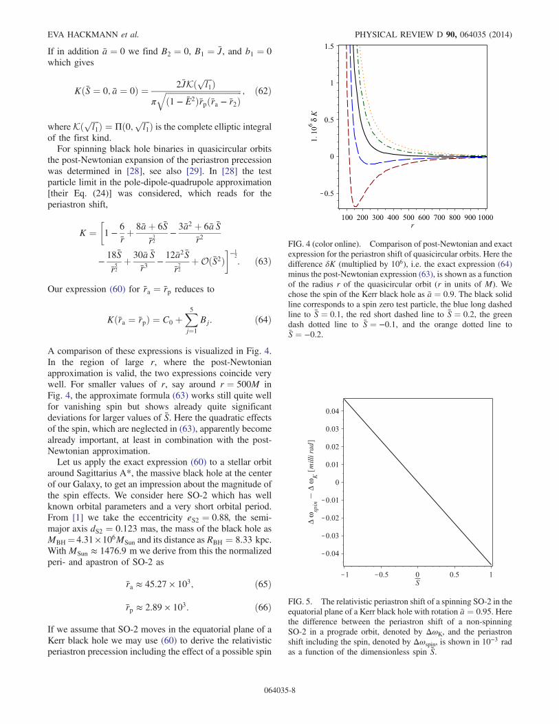
A comparison of these expressions is visualized in Fig. 4.In the region of large r, where the post-Newtonianapproximation is valid, the two expressions coincide verywell. For smaller values of r, say around r ¼ 500M inFig. 4, the approximate formula (63) works still quite wellfor vanishing spin but shows already quite significantdeviations for larger values of S. Here the quadratic effectsof the spin, which are neglected in (63), apparently becomealready important, at least in combination with the post-Newtonian approximation.Let us apply the exact expression (60) to a stellar orbit

around Sagittarius A*, the massive black hole at the centerof our Galaxy, to get an impression about the magnitude ofthe spin effects. We consider here SO-2 which has wellknown orbital parameters and a very short orbital period.From [1] we take the eccentricity eS2 ¼ 0.88, the semi-major axis dS2 ¼ 0.123 mas, the mass of the black hole asMBH ¼ 4.31×106MSun and its distance as RBH ¼ 8.33 kpc.WithMSun ≈ 1476.9 m we derive from this the normalizedperi- and apastron of SO-2 as

ra ≈ 45.27 × 103; ð65Þ

rp ≈ 2.89 × 103: ð66Þ

If we assume that SO-2 moves in the equatorial plane of aKerr black hole we may use (60) to derive the relativisticperiastron precession including the effect of a possible spin

FIG. 4 (color online). Comparison of post-Newtonian and exactexpression for the periastron shift of quasicircular orbits. Here thedifference δK (multiplied by 106), i.e. the exact expression (64)minus the post-Newtonian expression (63), is shown as a functionof the radius r of the quasicircular orbit (r in units of M). Wechose the spin of the Kerr black hole as a ¼ 0.9. The black solidline corresponds to a spin zero test particle, the blue long dashedline to S ¼ 0.1, the red short dashed line to S ¼ 0.2, the greendash dotted line to S ¼ −0.1, and the orange dotted line toS ¼ −0.2.

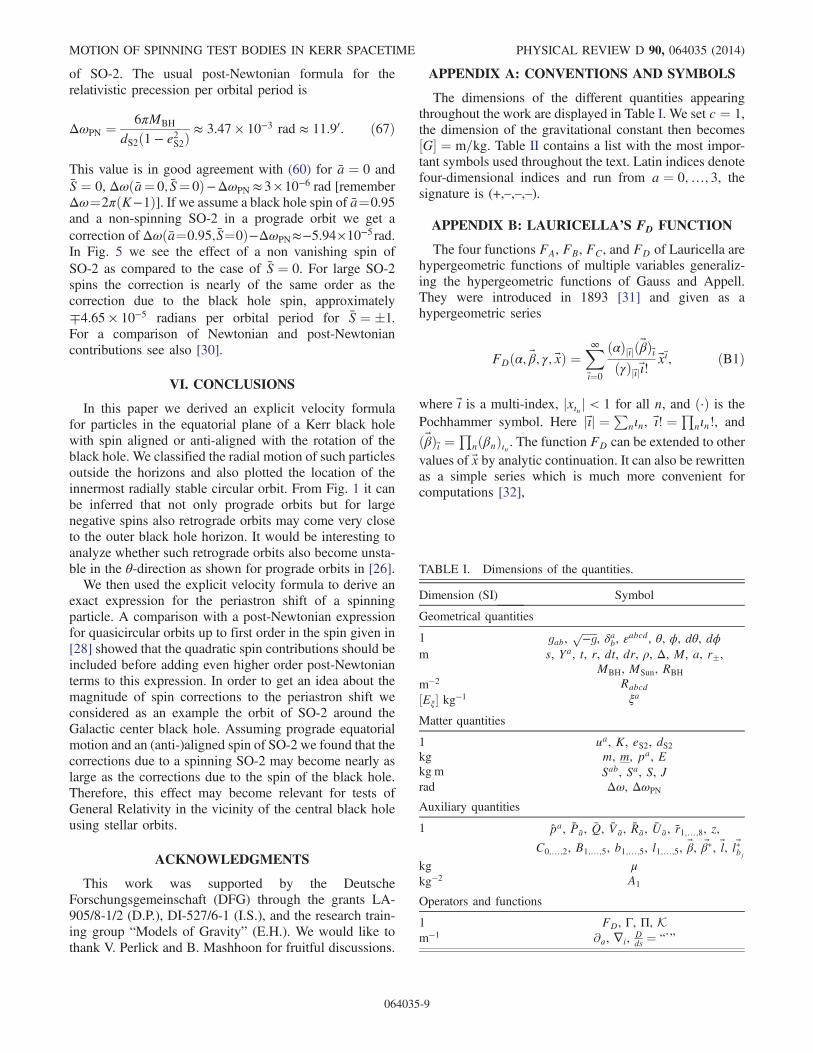
FIG. 5. The relativistic periastron shift of a spinning SO-2 in theequatorial plane of a Kerr black hole with rotation a ¼ 0.95. Herethe difference between the periastron shift of a non-spinningSO-2 in a prograde orbit, denoted by ΔωK, and the periastronshift including the spin, denoted by Δωspin, is shown in 10−3 radas a function of the dimensionless spin S.

EVA HACKMANN et al. PHYSICAL REVIEW D 90, 064035 (2014)

064035-8

of SO-2. The usual post-Newtonian formula for therelativistic precession per orbital period is

ΔωPN ¼ 6πMBH

dS2ð1 − e2S2Þ≈ 3.47 × 10−3 rad ≈ 11.90: ð67Þ

This value is in good agreement with (60) for a ¼ 0 andS ¼ 0, Δωða¼ 0; S¼ 0Þ−ΔωPN ≈ 3×10−6 rad [rememberΔω¼2πðK−1Þ]. If we assume a black hole spin of a¼0.95and a non-spinning SO-2 in a prograde orbit we get acorrection of Δωða¼0.95;S¼0Þ−ΔωPN≈−5.94×10−5 rad.In Fig. 5 we see the effect of a non vanishing spin ofSO-2 as compared to the case of S ¼ 0. For large SO-2spins the correction is nearly of the same order as thecorrection due to the black hole spin, approximately∓4.65 × 10−5 radians per orbital period for S ¼ �1.For a comparison of Newtonian and post-Newtoniancontributions see also [30].

VI. CONCLUSIONS

In this paper we derived an explicit velocity formulafor particles in the equatorial plane of a Kerr black holewith spin aligned or anti-aligned with the rotation of theblack hole. We classified the radial motion of such particlesoutside the horizons and also plotted the location of theinnermost radially stable circular orbit. From Fig. 1 it canbe inferred that not only prograde orbits but for largenegative spins also retrograde orbits may come very closeto the outer black hole horizon. It would be interesting toanalyze whether such retrograde orbits also become unsta-ble in the θ-direction as shown for prograde orbits in [26].We then used the explicit velocity formula to derive an

exact expression for the periastron shift of a spinningparticle. A comparison with a post-Newtonian expressionfor quasicircular orbits up to first order in the spin given in[28] showed that the quadratic spin contributions should beincluded before adding even higher order post-Newtonianterms to this expression. In order to get an idea about themagnitude of spin corrections to the periastron shift weconsidered as an example the orbit of SO-2 around theGalactic center black hole. Assuming prograde equatorialmotion and an (anti-)aligned spin of SO-2 we found that thecorrections due to a spinning SO-2 may become nearly aslarge as the corrections due to the spin of the black hole.Therefore, this effect may become relevant for tests ofGeneral Relativity in the vicinity of the central black holeusing stellar orbits.

ACKNOWLEDGMENTS

This work was supported by the DeutscheForschungsgemeinschaft (DFG) through the grants LA-905/8-1/2 (D.P.), DI-527/6-1 (I.S.), and the research train-ing group “Models of Gravity” (E.H.). We would like tothank V. Perlick and B. Mashhoon for fruitful discussions.

APPENDIX A: CONVENTIONS AND SYMBOLS

The dimensions of the different quantities appearingthroughout the work are displayed in Table I. We set c ¼ 1,the dimension of the gravitational constant then becomes½G� ¼ m=kg. Table II contains a list with the most impor-tant symbols used throughout the text. Latin indices denotefour-dimensional indices and run from a ¼ 0;…; 3, thesignature is (+,–,–,–).

APPENDIX B: LAURICELLA’S FD FUNCTION

The four functions FA, FB, FC, and FD of Lauricella arehypergeometric functions of multiple variables generaliz-ing the hypergeometric functions of Gauss and Appell.They were introduced in 1893 [31] and given as ahypergeometric series

FDðα; ~β; γ; ~xÞ ¼X∞~ι¼0

ðαÞj~ιjð~βÞ~ιðγÞj~ιj~ι!

~x~ι; ðB1Þ

where ~ι is a multi-index, jxιn j < 1 for all n, and ð·Þ is thePochhammer symbol. Here j~ιj ¼ P

nιn, ~ι! ¼Q

nιn!, and

ð~βÞ~ι ¼Q

nðβnÞιn . The function FD can be extended to othervalues of ~x by analytic continuation. It can also be rewrittenas a simple series which is much more convenient forcomputations [32],

TABLE I. Dimensions of the quantities.

Dimension (SI) Symbol

Geometrical quantities

1 gab,ffiffiffiffiffiffi−gp

, δab, εabcd, θ, ϕ, dθ, dϕ

m s, Ya, t, r, dt, dr, ρ, Δ, M, a, r�,MBH, MSun, RBH

m−2 Rabcd

½Eξ� kg−1 ξa

Matter quantities

1 ua, K, eS2, dS2kg m, m, pa, Ekg m Sab, Sa, S, Jrad Δω, ΔωPN

Auxiliary quantities

1 pa, Pa, Q, Va, Ra, Ua, r1;…;8, z,

C0;…;2, B1;…;5, b1;…;5, l1;…;5, ~β, ~β�, ~l, ~l�bjkg μkg−2 A1

Operators and functions

1 FD, Γ, Π, Km−1 ∂a, ∇i, D

ds ¼ “_”

MOTION OF SPINNING TEST BODIES IN KERR SPACETIME PHYSICAL REVIEW D 90, 064035 (2014)

064035-9

FDðα; ~β; γ; ~xÞ ¼ 1þX∞m¼1

ðαÞmðγÞm

Λm; ðB2Þ

where

Λm ¼Xj~ιj¼m

ð~βÞ~ι~ι!

~x~ι

¼X

f ~m∈NnjPj

mj¼mg

Ynj¼1

ðβjÞmj

mj!xmj

j : ðB3Þ

In this paper the FD function is used because it can berepresented in an integral form

FDðα; ~β; γ; ~xÞ ¼ΓðγÞ

ΓðαÞΓðγ − αÞ×Z

1

0

tα−1ð1 − tÞγ−α−1Yn

ð1 − xntÞ−βndt

ðB4Þ

for ReðγÞ > ReðαÞ > 0, where Γ denotes the gammafunction. It is a generalization of the Jacobian ellipticintegrals, e.g. πFDð1=2; 1=2; 1; k2Þ ¼ 2KðkÞ, where K isthe complete elliptic integral of the first kind.The constants appearing in front of FD in (60) are due to

a partial fraction decomposition of fðrðzÞÞ=ðrðzÞ − r1Þ2and given by

B1;2 ¼aðra − r1Þ

2Δðr1Þ3ða2 þ raðr1 − 2Þ þ ðra − r1Þr�Þð1 − r�Þ½ðJ − S EÞa7 − 2Eðr� þ 4r1 − 2Þa6

þ ½ð2J − E S−4ðJ − E SÞr1Þr� − 6ðJ − E SÞr21 þ 4ð2J − E SÞr1 − 4J�a5 þ 2Sa2ðJ − a EÞð2ðr1 − 1Þ3þ 2r�ðr1 − 1Þ2 þ r�r21 þ 2r1 − 2Þ þ r31ðJ − E SÞð4þ r1Þa3 − 2r31ðr1 þ 8ÞEr�a2þ ½ð12Er21 − J SÞr� þ 8Er31 − 4J S r1 þ 4J S�a4 − r41ð2J − 3E SÞr�aþ r41ð8E − J SÞr�� ðB5Þ

Bj ¼ fS2bjða EþS E−JÞðra − r1Þðrp − r1Þ=ðS2 þ r31Þ3ðra − rpÞ× ½ðra − rp þ bjðrp − r1ÞÞ2S2 þ r1ðr1ðrp − raÞ þ rabjðrp − r1ÞÞ2�g× ½ðra − rpÞ2r21ð10S4 − 16S2r31 þ r61Þ þ ðra − rpÞðrp − r1Þr1ð5ðra þ 3r1ÞS4 − 4r31ð5ra þ 3r1ÞS2 þ 2rar61Þbjþ ðrp − r1Þ2ððr2a þ 3rar1 þ 6r21ÞS4 − r31ð7ra þ 6rar1 þ 3r21ÞS2 þ r2a r61Þb2j �; ðB6Þ

where j ¼ 3, 4, 5 and r� ¼ 1�ffiffiffiffiffiffiffiffiffiffiffiffiffi1 − a2

pare the horizons, and the characteristics bj are solutions of the equations

TABLE II. Directory of symbols.

Symbol Explanation

Geometrical quantities

gab Metricffiffiffiffiffiffi−gpDeterminant of the metric

δab Kronecker symbolξa Killing vectort, r, θ, ϕ Coordinatess Proper timeYa World lineRabcd CurvatureM, a Kerr (mass, parameter)rþ, r− (outer, inner) horizonMBH, MSun Mass (black hole, Sun)RBH Distance to black hole

Matter quantities

ua Velocitym, m Mass (Frenkel, Tulczyjew)pa Generalized momentumEξ General conserved quantitySab, Sa, S Spin (tensor, vector, length)E, J Energy, angular momentumra, rp Apastron, periastronK, Δω, ΔωPN Periastron advance (dimensionless,

in rad, in PN-approximation)eS2, dS2 SO-2 eccentricity, semimajor axis

Operators and functions

εabcd Permutation symbol∂i, ∇i, D

ds ¼ “_” (Partial, covariant, total) derivative“¯” Dimensionless quantityFD Lauricella functionΓ Gamma functionK, Π Complete elliptic integrals

(first and third kind)

EVA HACKMANN et al. PHYSICAL REVIEW D 90, 064035 (2014)

064035-10

0 ¼ 2ðra − rpÞðrp − r1Þða2 − ra − r1 þ r1raÞbj þ ðrp − r1Þ2ΔðraÞb2j þ ðra − rpÞ2Δðr1Þ; ðB7Þ

for j ¼ 1, 2 and

0 ¼ ðra − rp þ bjðrp − r1ÞÞ3S2 þ ðr1ðra − rpÞ þ bjraðrp − r1ÞÞ3; ðB8Þ

for j ¼ 3, 4, 5. Furthermore we have

C2 ¼ðra − rpÞr1

Δðr1ÞðS2 þ r31Þðra − r1Þ2ðrp − r1Þ2½3ES2r1a3 þ ðES2ð1þ 3r1Þ − 3S J r1 þ Er31ÞSa2

− ðS3J þ S2Er21ð4 − 3r1Þ þ S J r31 − 2Er51Þaþ r21ðr1 − 2Þðr31 − 2S2ÞðJ − E SÞ�; ðB9Þ

C0 ¼1

Δðr1Þ3ðS2 þ r31Þ3ðra − r1Þ2½3ES2ðraS4 þ ð15rar1 − 7r2a − 6r21ÞS2 þ r61ðr2a þ 3r21 − 3rar1ÞÞa7

þ ðraE SðS6 þ ð45r1 þ 3Þr31S4 þ 3ð1 − 3r1Þr61S2 þ r91Þ − 9raS2Jr41ð5S2 − r31Þ− S2ðJ − E SÞð3r2a S4 − 3r31S

2ð7r2a þ 6r21Þ þ 3r61ðr2a þ 3r21ÞÞÞa6þ ðr1Eðð2r21 þ 9r1r2a − 12r2a − 6rar1ÞS6 − 3r31ð18r31 − 45rar21 − 38r21 þ 96rar1 þ 21r1r2a − 48r2aÞS4þ 3r71ð3r2a þ 12ra − 16r1 − 9rar1 þ 9r21ÞS2 þ 2r91ð3r2a þ r21 − 3rar1ÞÞ − J S raðS2 þ r31Þ3Þa5þ fEð8rar31 þ r31 þ 3r2a r21 − 6rar1 − 15r1r2a þ 2r2a − 3r41ÞS7 − Jr1ð−6rar1 þ 2r21 þ 8rar21 þ 3r1r2a − 3r31 − 12r2aÞS6− 3Er31ð27r2a r21 − 45r1r2a þ 6rar1 þ 21r41 − 2r2a − 37r31 − 53rar31 þ 90rar21ÞS5þ 3Jr41ð27r1r2a þ 21r31 − 48r2a þ 96rar1 − 53rar21 − 38r21ÞS4 þ 3r81Jð−6r21 þ 3r2a þ rar1 − 12ra þ 16r1ÞS2− 3Er61ð6rar1 − 6r41 − 2r2a þ 17r31 þ 3r1r2a þ 3r2a r21 þ rar31 − 18rar21ÞS3− Er91ð3r41 þ 6r2a r21 − r31 − 3r1r2a þ 6rar1 − 2r2a − 8rar31ÞSþ Jr101 ð6r1r2a − 6r2a − 2r21 þ 3r31 − 8rar21 þ 6rar1Þga4þ fEr21ð−6r121 þ 4rar101 þ 4S6rar1 − 42S2r2a r71 − 126S2r91 − 216S4r51 þ 108S2r81 − 504S4rar51 þ 552S4rar41

þ 144S2rar81 − 96S2rar71 − 12r2a r91 − 6S6r31 − 2r2a r101 þ 12S6rar21 þ 135S4rar61 − 63S4r2a r51

− 27S2rar91 þ 9S2r2a r81 þ 27S2r101 þ 12rar111 − 54S4r71 þ 9S6r2a r21 þ 24S6r2a þ 246S4r2a r41 − 38S6r2a r1

þ 198S4r61 − 288S4r2a r31Þ þ J SðS2 þ r31Þ3ð−6rar21 þ 6rar1 − 2r2a þ 3r1r2a þ r31Þga3þ fEr21ð6rar1 − 9rar21 þ 24r2a − 21r1r2a þ r41 þ 3r31 þ 4r1 þ 6r2a r21 − 6r21ÞS7 − Jr21ð−22r1r2a þ 24r2a þ 4rar1

þ r41 þ 6r2a r21 − 6rar21ÞS6 − 3Er51ð17r41 þ 189rar21 − 45rar31 − 186rar1 − 99r1r2a þ 96r2a þ 24r2a r21 − 4r1

− 75r31 þ 78r21ÞS5 þ 3Jr51ð−45rar31 − 98r1r2a þ 72r21 þ 24r2a r21 − 72r31 − 184rar1 þ 96r2a þ 17r41 þ 186rar21ÞS4þ 3Er91ð−30ra − 33r21 þ 4þ 27rar1 þ 30r1 þ 10r31 − 9rar21 þ 3r2aÞS3 − 3Jr91ð2r2a − 32ra þ 36r1 − 36r21

þ 30rar1 þ 10r31 − 9rar21ÞS2 − Er111 ð−3r31 þ 12r2a − r41 − 15r1r2a þ 6r21 þ 3r2a r21 − 4r1 − 6rar1 þ 9rar21ÞSþ Jr111 ð−r41 − 14r1r2a þ 3r2a r21 þ 12r2a − 4rar1 þ 6rar21Þga2þ fr31ð4r121 þ 2rar121 þ 36S2r2a r71 þ 120S2r91 þ 144S4r51 − 72S2r81 þ 504S4rar51 − 360S4rar41 − 144S2rar81

þ 72S2rar71 þ 9S2r111 − 18S4r81 þ 2S6rar31 þ 8r2a r91 þ 4S6r31 − 12S6rar21 − 264S4rar61 þ 126S4r2a r51

þ 60S2rar91 − 18S2r2a r81 − 54S2r101 − 12rar111 þ 108S4r71 − 18S6r2a r21 − 21S4r2a r61 þ 45S4rar71 þ 3S6r2a r31

− 9S2rar101 þ 3S2r2a r91 − 16S6r2a − 252S4r2a r41 þ 36S6r2a r1 − 204S4r61 þ 192S4r2a r31ÞE − r31J Sð2ra − 3rar1

þ r2a þ 3r21 þ 4 − 6r1ÞðS2 þ r31Þ3ga− r31ðr1 − 2Þ3ð−r2a r91 þ 9S2r81 − 9S2rar71 − 18S4r51 þ 45S4rar41 − 24S4r2a r31 þ 2S6r2aÞðJ − E SÞ�; ðB10Þ

MOTION OF SPINNING TEST BODIES IN KERR SPACETIME PHYSICAL REVIEW D 90, 064035 (2014)

064035-11

C1 ¼ðra − rpÞ

Δðr1Þ2ðS2 þ r31Þ2ðra − r1Þ2ðrp − r1Þ½3ES2r1ð2raS2 þ 3r41 − 2rar31Þa5

þ ðES4ðra þ r1 þ 6rar1Þ− 6Jr1raS3 þ Er31ð9r21 þ 2r1 þ 2ra − 3rar1ÞS2 þ 3Jr41ðra − 3r1ÞSþ Er61ðra þ r1ÞÞSa4þ ð2Er21ðr61ð3ra − r1Þ þ ð9r21 − 20r1 þ 12ra − 3rar1Þr31S2 − S4ð9ra þ r1 − 6rar1ÞÞ− J SðS2 þ r31Þ2ðra þ r1ÞÞa3þ ðEð2r21 þ r1 − 19ra þ 8rar1 − 4ÞS5 − 2Jðr21 − r1 − 9ra þ 4rar1ÞS4 þ 2Er31ð11r21 − 17r1 þ 11ra − 7rar1 − 4ÞS3− 2Jr31ð11r21 − 20r1 þ 12ra − 7rar1ÞS2 þ Er61ð2r21 þ r1 þ 5ra − 4rar1 − 4ÞS− 2Jr61ðr21 − r1 þ 3ra − 2rar1ÞÞr21a2þ ðEr1ð2ðr21 þ 3rar21 þ 8ra − 11rar1ÞS4 þ r31ð9r31 − 32r21 − 3rar21 þ 16rar1 þ 36r1 − 28raÞS2 þ 2r61ðr21 þ rar1 − 4raÞÞþ J SðS2 þ r31Þ2ðra − 3r1 þ 4ÞÞr21a− r31ðr1 − 2Þ2ðJ − E SÞð9S2r41 þ rað4S2 þ r31ÞðS2 − 2r21ÞÞ�: ðB11Þ

[1] S. Gillessen, F. Eisenhauer, S. Trippe, T. Alexander, R.Genzel, F. Martins, and T. Ott, Astrophys. J. 692, 1075(2009).

[2] R. Genzel, F. Eisenhauer, and S. Gillessen, Rev. Mod. Phys.82, 3121 (2010).

[3] http://www.skatelescope.org.[4] M. Mathisson, Acta Phys. Pol. 6, 163 (1937).[5] A. Papapetrou, Proc. R. Soc. A 209, 248 (1951).[6] W. Tulczyjew, Acta Phys. Pol. 18, 393 (1959).[7] W. G. Dixon, Nuovo Cimento 34, 317 (1964).[8] W. G. Dixon, Phil. Trans. R. Soc. A 277, 59 (1974).[9] V. Z. Enolskii, E. Hackmann, V. Kagramanova, J. Kunz, and

C. Lämmerzahl, J. Geom. Phys. 61, 899 (2011).[10] V. Z. Enolskii, B. Hartmann, V. Kagramanova, J. Kunz, C.

Lämmerzahl, and P. Sirimachan, J. Math. Phys. (N.Y.) 53,012504 (2012).

[11] J. Steinhoff and D. Puetzfeld, Phys. Rev. D 81, 044019(2010).

[12] J. Ehlers and E. Rudolph, Gen. Relativ. Gravit. 8, 197(1977).

[13] Y. N. Obukhov and D. Puetzfeld, Phys. Rev. D 83, 044024(2011).

[14] C. Chicone, B. Mashhoon, and B. Punsley, Phys. Lett. A343, 1 (2005).

[15] B. Mashhoon and D. Singh, Phys. Rev. D 74, 124006(2006).

[16] D. Singh, Gen. Relativ. Gravit. 40, 1179 (2008).[17] D. Singh, Phys. Rev. D 78, 104028 (2008).[18] L. I. Schif, Phys. Rev. Lett. 4, 215 (1960).[19] C. W. F. Everitt et al., Phys. Rev. Lett. 106, 221101 (2011).[20] O. Semerák, Mon. Not. R. Astron. Soc. 308, 863 (1999).[21] K. Kyrian and O. Semerák, Mon. Not. R. Astron. Soc. 382,

1922 (2007).[22] R. Plyatsko and M. Fenyk, Phys. Rev. D 87, 044019

(2013).[23] J. Steinhoff and D. Puetzfeld, Phys. Rev. D 86, 044033

(2012).[24] A. García, E. Hackmann, J. Kunz, C. Lämmerzahl, and A.

Macias, arXiv:1306.2549.[25] Y. Mino, Phys. Rev. D 67, 084027 (2003).[26] S. Suzuki and K. Maeda, Phys. Rev. D 58, 023005

(1998).[27] K. P. Tod, F. De Felice, and M. Calvani, Nuovo Cimento B

34, 365 (1976).[28] A. Le Tiec et al. Phys. Rev. D 88, 124027 (2013).[29] M. Tessmer, J. Hartung, and G. Schäfer, Classical Quantum

Gravity 30, 015007 (2013).[30] G. Rubilar and A. Eckart, Astron. Astrophys. 374, 95

(2001).[31] G. Lauricella, Rend. Circ. Math. Palermo 7, 111 (1893).[32] P. van Laarhoven and T. Kalker, J. Comput. Appl. Math. 21,

369 (1988).

EVA HACKMANN et al. PHYSICAL REVIEW D 90, 064035 (2014)

064035-12