Embed Size (px)
Citation preview
HAL Id: lirmm-01718243https://hal-lirmm.ccsd.cnrs.fr/lirmm-01718243
Submitted on 15 Mar 2018
HAL is a multi-disciplinary open accessarchive for the deposit and dissemination of sci-entific research documents, whether they are pub-lished or not. The documents may come fromteaching and research institutions in France orabroad, or from public or private research centers.
L’archive ouverte pluridisciplinaire HAL, estdestinée au dépôt et à la diffusion de documentsscientifiques de niveau recherche, publiés ou non,émanant des établissements d’enseignement et derecherche français ou étrangers, des laboratoirespublics ou privés.
Motion Control of a Hovering Biomimetic Four-FinUnderwater Robot
Taavi Salumäe, Ahmed Chemori, Maarja Kruusmaa
To cite this version:Taavi Salumäe, Ahmed Chemori, Maarja Kruusmaa. Motion Control of a Hovering Biomimetic Four-Fin Underwater Robot. IEEE Journal of Oceanic Engineering, Institute of Electrical and ElectronicsEngineers, 2019, 44 (1), pp.54-71. �10.1109/JOE.2017.2774318�. �lirmm-01718243�
1
Motion Control of a Hovering Biomimetic
4-fin Underwater Robot
Taavi Salumae, Ahmed Chemori, and Maarja Kruusmaa
Abstract
U-CAT is a highly maneuverable biomimetic 4-fin underwater robot for operating in confined spaces.
Because of its novel mechanical design and specialized purpose, the traditional autonomous underwater
robot control methods are not directly applicable on U-CAT. This paper proposes a novel modular control
architecture that can be adopted for different application scenarios. Within this framework we implement
and test several 2-degree of freedom (DOF) controllers and discuss the test results. Furthermore, we
describe and implement an actuation coupling method by prioritizing the selection of DOF with fuzzy
membership functions and demonstrate the approach for 3-DOF control. The results show that the
proposed DOF prioritization approach helps to improve tracking both in the case of human in the loop
and automatic control. Finally, we describe long duration field experiments in realistic environmental
conditions.
I. INTRODUCTION
AUTONOMOUS underwater vehicles (AUVs), such as Iver-2 [1], Bluefins [2] and Remus
[3], are nowadays widely used in many research areas and industries. For example the
oil and gas industry uses them for surveys to locate deposits and to inspect pipelines or rigs
[4], navies use them for intelligence and mine countermeasures [5]; and archaeologists use
them to locate historical shipwrecks [6]. The large variety of applications of AUVs motivates
researchers to develop more and more advanced control systems and technologies for these
vehicles. The more advanced control systems in turn shift AUV application towards even more
complex underwater environments. In many of these environments, traditional vehicle designs
Taavi Salumae and Maarja Kruusmaa are with Centre for Biorobotics, Tallinn University of Technology, Tallinn, Estonia,
Ahmed Chemori is with LIRMM UMR CNRS/Univ. of Montpellier, 161 rue Ada, 34392 Montpellier, France,
2
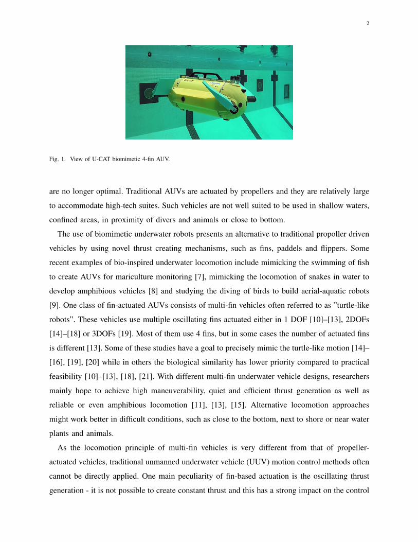
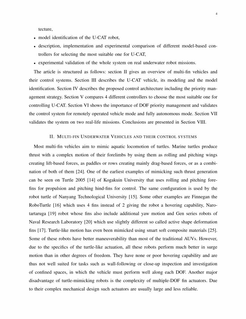
Fig. 1. View of U-CAT biomimetic 4-fin AUV.
are no longer optimal. Traditional AUVs are actuated by propellers and they are relatively large
to accommodate high-tech suites. Such vehicles are not well suited to be used in shallow waters,
confined areas, in proximity of divers and animals or close to bottom.
The use of biomimetic underwater robots presents an alternative to traditional propoller driven
vehicles by using novel thrust creating mechanisms, such as fins, paddels and flippers. Some
recent examples of bio-inspired underwater locomotion include mimicking the swimming of fish
to create AUVs for mariculture monitoring [7], mimicking the locomotion of snakes in water to
develop amphibious vehicles [8] and studying the diving of birds to build aerial-aquatic robots
[9]. One class of fin-actuated AUVs consists of multi-fin vehicles often referred to as ”turtle-like
robots”. These vehicles use multiple oscillating fins actuated either in 1 DOF [10]–[13], 2DOFs
[14]–[18] or 3DOFs [19]. Most of them use 4 fins, but in some cases the number of actuated fins
is different [13]. Some of these studies have a goal to precisely mimic the turtle-like motion [14]–
[16], [19], [20] while in others the biological similarity has lower priority compared to practical
feasibility [10]–[13], [18], [21]. With different multi-fin underwater vehicle designs, researchers
mainly hope to achieve high maneuverability, quiet and efficient thrust generation as well as
reliable or even amphibious locomotion [11], [13], [15]. Alternative locomotion approaches
might work better in difficult conditions, such as close to the bottom, next to shore or near water
plants and animals.
As the locomotion principle of multi-fin vehicles is very different from that of propeller-
actuated vehicles, traditional unmanned underwater vehicle (UUV) motion control methods often
cannot be directly applied. One main peculiarity of fin-based actuation is the oscillating thrust
generation - it is not possible to create constant thrust and this has a strong impact on the control
3
stability. The thrust vector of fins is also much less reactive. While the rotation speed of the
propeller can usually be changed in a fraction of a second, the thrust of a fin depends on the
oscillation amplitude and frequency which cannot be changed equally fast. Moreover, the thrust
of fins cannot be as easily and precisely estimated as it is a complex function between oscillation
parameters, bending modes and harmonic oscillations of fins and other variables. Next, and likely
the biggest difference between highly maneuverable traditional UUVs and multi-fin UUVs, is
that the former usually use a separate actuator for controlling each degree of freedom whereas the
latter are mostly under-actuated. Multi-fin UUVs instead use different combinations of actuator
configurations in order to achieve motion in the available DOFs. This creates strong coupling
between the control of different DOFs. For example, when such a vehicle is diving at full speed,
the fins are pointed straight up. This configuration completely prevents a surge action to be done
at the same time, as this requires the fins to be oriented horizontally.
In this paper we propose a motion control system for biomimetic vehicles actuated by 4
pitching fins. We demonstrate the implementation and functionality of the motion control system
on a novel 4-fin biomimetic AUV U-CAT (Fig. 1). U-CAT is an agile 6-DOF maneuverable
vehicle developed for autonomous and semi-autonomous inspection of confined spaces, such as
shipwrecks, caves, submerged buildings etc. With regards to the mechanical locomotion principle,
U-CAT presents a slight departure from previous works; in task/mission directive, the vehicle
is fully novel. We propose a control architecture suitable for semi-autonomous and autonomous
control of the vehicle, more specifically:
• a modular, easily extensible control architecture that allows rapid and simple implementation
and testing of different controllers for different control scenarios.
• comparison of four controllers for simultaneous control of 2 DOFs
• a method for dealing with actuation coupling by prioritizing the action of different DOFs
• simultaneous control of 3 DOFs in 1) manual control with 2 DOF autopiloting, i.e. remotely
operated vehicle (ROV) mode; 2) fully autonomous control (AUV mode)
• demonstration and validation of the performance for a real underwater mission
This paper build upon our previous work published on IEEE conferences [22] and [23]. These
articles have outlined our approach to the control architecture along with partial test results. This
paper extends the conference articles by adding:
• more detailed description of the implementation and validation of the whole control archi-
4
tecture,
• model identification of the U-CAT robot,
• description, implementation and experimental comparison of different model-based con-
trollers for selecting the most suitable one for U-CAT,
• experimental validation of the whole system on real underwater robot missions.
The article is structured as follows: section II gives an overview of multi-fin vehicles and
their control systems. Section III describes the U-CAT vehicle, its modeling and the model
identification. Section IV describes the proposed control architecture including the priority man-
agement strategy. Section V compares 4 different controllers to choose the most suitable one for
controlling U-CAT. Section VI shows the importance of DOF priority management and validates
the control system for remotely operated vehicle mode and fully autonomous mode. Section VII
validates the system on two real-life missions. Conclusions are presented in Section VIII.
II. MULTI-FIN UNDERWATER VEHICLES AND THEIR CONTROL SYSTEMS
Most multi-fin vehicles aim to mimic aquatic locomotion of turtles. Marine turtles produce
thrust with a complex motion of their forelimbs by using them as rolling and pitching wings
creating lift-based forces, as paddles or rows creating mainly drag-based forces, or as a combi-
nation of both of them [24]. One of the earliest examples of mimicking such thrust generation
can be seen on Turtle 2005 [14] of Kogakuin University that uses rolling and pitching fore-
fins for propulsion and pitching hind-fins for control. The same configuration is used by the
robot turtle of Nanyang Technological University [15]. Some other examples are Finnegan the
RoboTurtle [16] which uses 4 fins instead of 2 giving the robot a hovering capability, Naro-
tartaruga [19] robot whose fins also include additional yaw motion and Gen series robots of
Naval Research Laboratory [20] which use slightly different so called active shape deformation
fins [17]. Turtle-like motion has even been mimicked using smart soft composite materials [25].
Some of these robots have better maneuverability than most of the traditional AUVs. However,
due to the specifics of the turtle-like actuation, all these robots perform much better in surge
motion than in other degrees of freedom. They have none or poor hovering capability and are
thus not well suited for tasks such as wall-following or close-up inspection and investigation
of confined spaces, in which the vehicle must perform well along each DOF. Another major
disadvantage of turtle-mimicking robots is the complexity of multiple-DOF fin actuators. Due
to their complex mechanical design such actuators are usually large and less reliable.
5
U-CAT generates thrust by using only the pitching motion of fins. This allows us to reduce
complexity and size of the fins as each fin is driven only by a single motor. Pitching fins have
previously been used also on Madeleine of Nekton Research [10], [26], its commercial successor,
an amphibian ROV Transphibian of IRobot [11] and a vehicle developed by Robotics Institute of
Beihang University [12]. All these vehicles have 4 pitching fins whose rotation axes are parallel
[10] or very close to parallel [11], [12]. Such fin configuration allows to control the robots in
maximum 5 DOFs, leaving out the sway motion i.e. they can not move sideways. U-CAT, on the
contrary, has a different mechanical configuration that also makes the sideways motion possible,
thus giving the vehicle all 6 controllable DOFs.
There are also some other, slightly different vehicles that use pitching fins. An amphibious
robot of Peking University [21] uses fins that are actuated by two parallel motors through a
special five-bar link mechanism. The mechanism allows the fins to be used for thrust generation
or as legs for walking on the ground. Another vehicle of Peking University [18] has fins whose
rotation axes can be reoriented using 4 additional motors. This vehicle is extremely highly
maneuverable and can be used to control 6 DOFs, but this comes at a price of doubling the
number of motors. The amphibious Aqua vehicle of McGill University [13] uses 6 pitching fins
instead of 4. The additional two fins help to improve the crawling performance, but are excessive
when only aquatic locomotion is desired.
Motion control systems of most of multi-fin vehicles are not as profoundly developed as
their mechanical designs, however, there are some exceptions. Many of the authors have only
presented open-loop or manual control [12], [14], [15], [18], [21]. Their main contribution lies in
the development and analysis of the gait generation, for example using central pattern generators
[12], [18], [21]. Some studies have been conducted about the control of non-hover-capable turtle-
like vehicles during dominant surge motion. [20] demonstrates model free control for only 1 DOF
at the same time, [19] presents model free control of the angular rate for forward swimming
stabilization. [16] concentrates mostly on mimicking the fin kinematics and maneuvering of
a biological turtle on Finnegan the RoboTurtle, but it presents also results on pitch, roll and
yaw control for different dynamically stable and unstable turning maneuvers. To the best of our
knowledge, there are no studies that concentrate on the automatic position control of 4-fin hover-
capable vehicles. Although [10] claims to have a simultaneous control of different DOFs of the
Madeleine vehicle, the authors have not published the control approach or any experimental or
simulated results yet.
6
Advanced position control has been developed for a 6-fin amphibious Aqua vehicle [13]. It is
somewhat similar to the U-CAT in terms of using only pitching fins and being hover-capable. [27]
and [28] present modeling and model-based control of Aqua, but only for a single simultaneous
DOF. In [29] authors also demonstrate multi-DOF control using a combination of model-free PD
and PI controllers for yaw, roll, pitch and heave. They avoid coupling problems by using gain
scheduling depending on the surge speed. Even though authors have reported good trajectory
following, this was achieved by tuning an array of 45 control parameters, making the developed
control approach complex and inextensible. Authors have tried to simplify the process by using
online gain adaption algorithms [30], however the presented results show large deviations from
desired attitude.
As it can be seen from the background overview, many different fin-actuated vehicles have
been developed in recent years. However, the control of these vehicles, especially the position
control of hover-capable vehicles is relatively little studied.
III. U-CAT VEHICLE
U-CAT is a biomimetic underwater vehicle designed for autonomous and semi-autonomous
inspection of confined areas, such as shipwrecks, caves and man-made underwater structures. It
was developed in the framework of the European Commission funded research project ARROWS
[31]. The aim of ARROWS project was to adapt and develop low-cost AUV technologies to
significantly reduce the cost of archaeological operations. U-CAT was designed specifically
to meet archaeologists’ requirements for unmanned shipwreck penetration. It uses fin-based
locomotion to achieve high maneuverability and for quiet and safe locomotion. One unique
feature of U-CAT compared to other mentioned 4-fin vehicles lies in its fin configuration. The
fins are placed such that a thrust force can be created in all the 6 DOFs. This includes sway, which
cannot be controlled with other vehicles using 1 DOF pitching fins, but which is extremely useful
for various video inspection tasks such as wall following. More detailed design justification and
the description of vehicle are presented in [32]. Some preliminary control results for 1 degree
of freedom using non-model-based controllers are published in [22].
U-CAT is 56 cm long and weights approximately 19 kg. Its four fins are actuated by 60 W
Maxon brushless DC motors driven by Maxon Epos motor drivers using sensorless back-EMF
feedback control. The vehicle has an internal battery allowing at least 6 hours of autonomous
operation. The whole control architecture is developed on an internal single-board computer
7
zb
xb
ϑ
ψ
ϕ
yb
xe ze
ye xyz
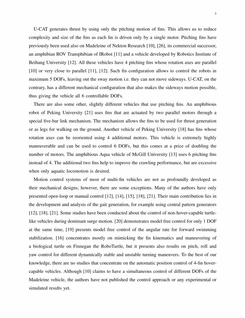
Fig. 2. Coordinate systems used in this study. {xb, yb, zb} is the body-fixed coordinate frame and {xe, ye, eb} is the earth-fixed
coordinate frame. Robot’s position is presented as a vector of positions in earth-fixed frame η = [x, y, z, ϕ, ϑ, ψ]T
with ARM Cortex A9 quad-core 1Ghz processor. We use a modular development approach with
ROS middleware. The on-board computer communicates with a remote PC through a custom
connectorless tether mounted on top of the vehicle. In the end of the tether there is a waterproofed
WiFi router, creating an ultra short range underwater WiFi link. We use the remote PC only for
forwarding remote controller actions in ROV mode, and accessing the on-board computer for
debugging. As a remote controller we used a Sony Playstation DualShock 3.
In this paper we use the following sensors of U-CAT:
• Invensense MPU-6050 IMU for measuring the robot’s attitude. In the current study only yaw
measurement is directly used as a feedback in control loop. The roll and pitch measurements
are used only for coordinate transformations. The sampling frequency is 5 Hz.
• GEMS 3101 analog output pressure sensor with 18-bit DAQ for measuring depth. The
sampling frequency is 10 Hz and the resolution is 0.6 mm.
U-CAT has some additional devices not used in this study, but which will be used in fur-
ther developments: Applicon acoustic modem for underwater communication and localization;
two active buoyancy control modules; custom-developed hydrophone array for acoustic beacon
localization; custom-made echosounder array for close-distance obstacle avoidance; Point Grey
Chameleon camera; and various system health monitoring sensors.
A. Kinematics
U-CAT has four fins placed at 30 degree angle with respect to the vehicles center-line on
the horizontal plane. Each fin i is separately actuated using a sinusoidal input with parameters:
8
a) b) c)
d) e) f)
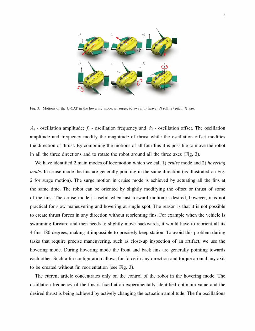
Fig. 3. Motions of the U-CAT in the hovering mode: a) surge; b) sway; c) heave; d) roll; e) pitch; f) yaw.
Ai - oscillation amplitude; fi - oscillation frequency and Φi - oscillation offset. The oscillation
amplitude and frequency modify the magnitude of thrust while the oscillation offset modifies
the direction of thrust. By combining the motions of all four fins it is possible to move the robot
in all the three directions and to rotate the robot around all the three axes (Fig. 3).
We have identified 2 main modes of locomotion which we call 1) cruise mode and 2) hovering
mode. In cruise mode the fins are generally pointing in the same direction (as illustrated on Fig.
2 for surge motion). The surge motion in cruise mode is achieved by actuating all the fins at
the same time. The robot can be oriented by slightly modifying the offset or thrust of some
of the fins. The cruise mode is useful when fast forward motion is desired, however, it is not
practical for slow maneuvering and hovering at single spot. The reason is that it is not possible
to create thrust forces in any direction without reorienting fins. For example when the vehicle is
swimming forward and then needs to slightly move backwards, it would have to reorient all its
4 fins 180 degrees, making it impossible to precisely keep station. To avoid this problem during
tasks that require precise maneuvering, such as close-up inspection of an artifact, we use the
hovering mode. During hovering mode the front and back fins are generally pointing towards
each other. Such a fin configuration allows for force in any direction and torque around any axis
to be created without fin reorientation (see Fig. 3).
The current article concentrates only on the control of the robot in the hovering mode. The
oscillation frequency of the fins is fixed at an experimentally identified optimum value and the
desired thrust is being achieved by actively changing the actuation amplitude. The fin oscillations

9
are synchronized to have a zero phase shift. Precise synchronization is important to reduce
irregular motions of the vehicle resulting from oscillating thrust vectors. When the fins are all
oscillating in the same phase, the vehicle oscillates mostly in the heave direction.
B. Dynamics
We model the rigid body dynamics of the vehicle in 6 DOFs using Fossen’s robot-like vectorial
model of marine craft [33]. The Fossen’s model is well suited for computer implementation and
control systems design. Therefore it is widely used in underwater robotics, but also in submarine
and surface vessel studies. The 6 DOF model is represented as:
Mν +C(ν)ν +D(ν)ν + g(η) = τ (1)
η = J(η)ν (2)
where η = [x, y, z, ϕ, ϑ, ψ]T is the vector of positions and orientations in the earth-fixed frame,
ν = [u, v, w, p, q, r]T is the vector of linear and angular velocities in the body-fixed frame and
J(η) ∈ R6×6 is the transformation matrix mapping from the body-fixed frame to the earth-
fixed frame. The systems coordinates are presented on Fig. 2. M =MRB +MA is the system
inertia matrix, where MRB is the inertia matrix of the vehicle and MA describes the added mass
resulting from the accelerating volume of water surrounding the robot. C(ν) = CRB +CA is
the Coriolis-centripetal matrix which again takes into account the rigid body and the added mass.
D(ν) is the damping matrix, g(η) is the vector of gravitational/buoyancy forces and moments
and τ = [X, Y, Z,K,M,N ]T is the vector of control inputs. τ can be represented as a resultant
force composed of forces Fi with which each fin i acts on the rigid body.
C. Fin forces
To successfully control the vehicle using model-based approaches, we need to know the
relationship between the fin actuation parameters and the generated thrust force. The forces
generated by the fins depend on complex interactions between the viscoelastic body and the
hydrodynamics of the surrounding water. We have previously studied the analytical modeling
of these interactions [34], however, due to complex nature of the system, analytical models
are either too imprecise or not suitable for using in real-time control. Therefore, we create an
empirical model of the fin thrust.
10
Amplitude, deg0 10 20 30 40 50 60
Mea
n Th
rust
, N
0
1
2
3
4 2.3 Hz
0.5 Hz
1.4 Hz
0.8 Hz
1.1 Hz
2.6 Hz1.7 Hz
2.0 Hz
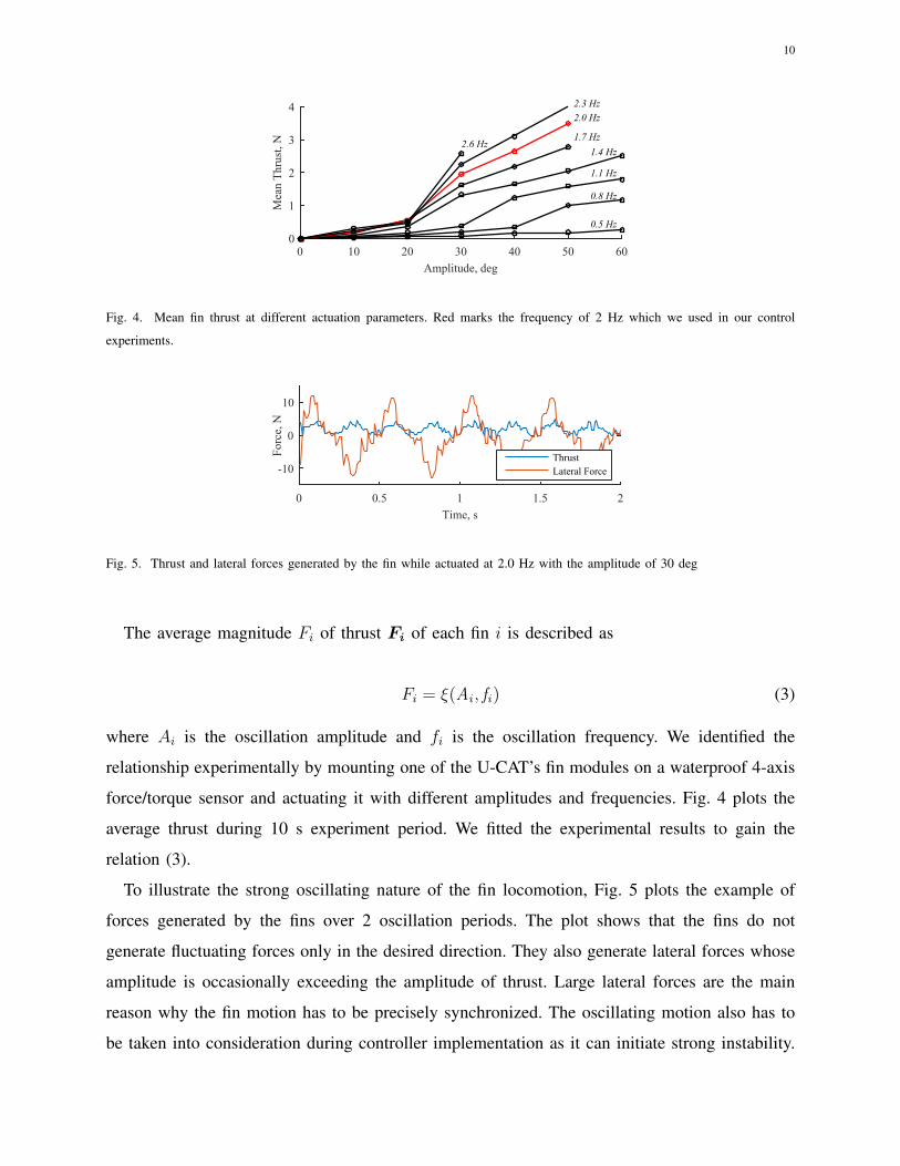
Fig. 4. Mean fin thrust at different actuation parameters. Red marks the frequency of 2 Hz which we used in our control
experiments.
Time, s0 0.5 1 1.5 2
Forc
e, N
-10
0
10
ThrustLateral Force
Fig. 5. Thrust and lateral forces generated by the fin while actuated at 2.0 Hz with the amplitude of 30 deg
The average magnitude Fi of thrust Fi of each fin i is described as
Fi = ξ(Ai , fi) (3)
where Ai is the oscillation amplitude and fi is the oscillation frequency. We identified the
relationship experimentally by mounting one of the U-CAT’s fin modules on a waterproof 4-axis
force/torque sensor and actuating it with different amplitudes and frequencies. Fig. 4 plots the
average thrust during 10 s experiment period. We fitted the experimental results to gain the
relation (3).
To illustrate the strong oscillating nature of the fin locomotion, Fig. 5 plots the example of
forces generated by the fins over 2 oscillation periods. The plot shows that the fins do not
generate fluctuating forces only in the desired direction. They also generate lateral forces whose
amplitude is occasionally exceeding the amplitude of thrust. Large lateral forces are the main
reason why the fin motion has to be precisely synchronized. The oscillating motion also has to
be taken into consideration during controller implementation as it can initiate strong instability.
11
D. Model identification
The initial dynamic parameters in (1) were found using both analytical and computational
methods. Using experimental model identification, the most important of these parameters were
adjusted.
The geometrical properties of the vehicle are found from a detailed 3D model drawn in
SolidWorks CAD software. The model includes all the internal and external components of
the robot and also the density of the larger components. The 3D model allowed us to precisely
calculate all the components of the U-CAT’s inertia matrix MRB, the Coriolis-centripetal matrix
CRB, and the gravity and buoyancy vector g(η). The damping is modeled as a hydrodynamic
drag. The drag coefficients in the damping matrix D(ν) are found using a computational fluid
dynamics package called Solidworks Flow Simulation. The inertia MA and Coriolis-centripetal
matrix CA of the added mass are calculated with the help of strip theory [35] using simplified
geometrical representation of the vehicle. Strip theory is a widely used approach in marine
engineering. It can be used to find an added mass of closed 2D contours. The added mass of
contours is summed to find the added mass of the whole body.
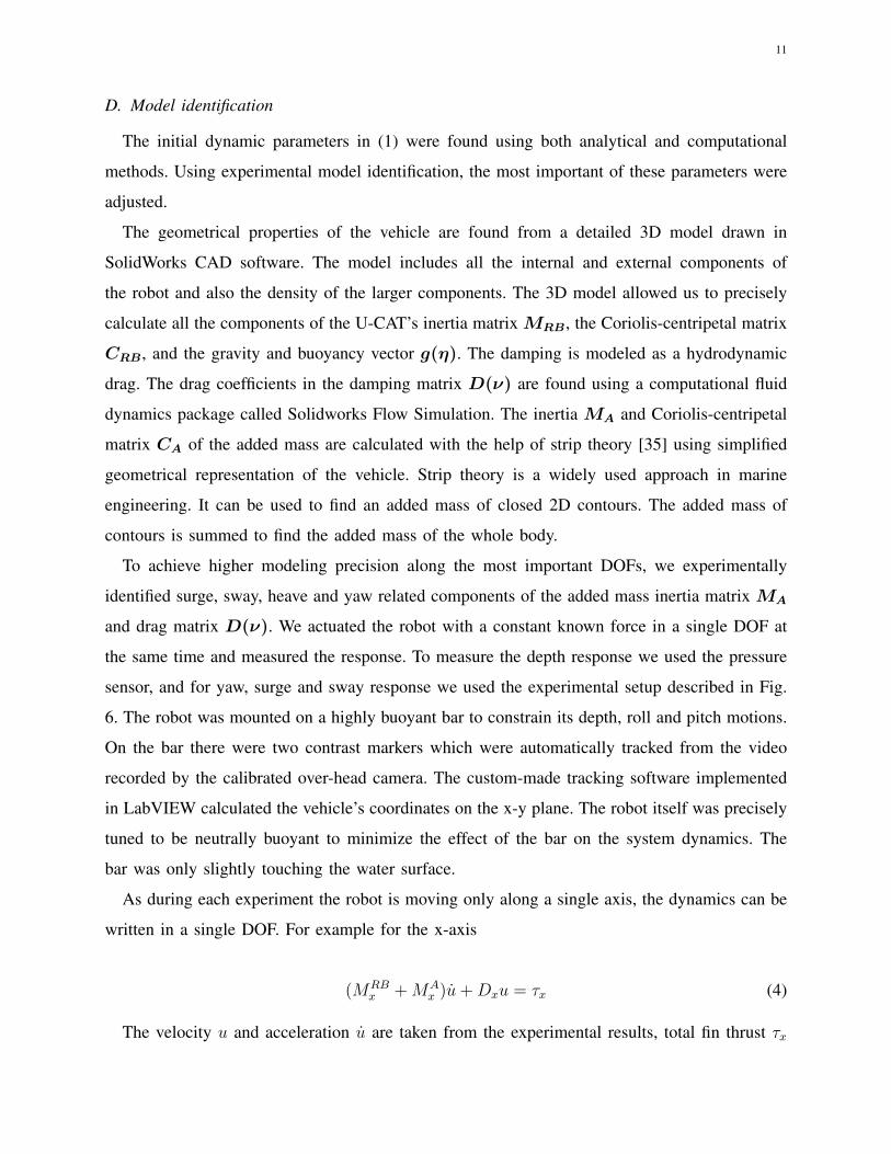
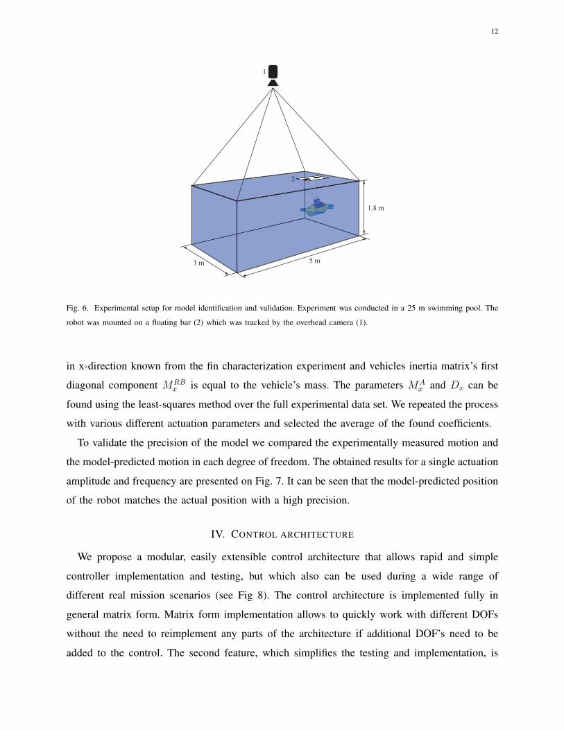
To achieve higher modeling precision along the most important DOFs, we experimentally
identified surge, sway, heave and yaw related components of the added mass inertia matrix MA
and drag matrix D(ν). We actuated the robot with a constant known force in a single DOF at
the same time and measured the response. To measure the depth response we used the pressure
sensor, and for yaw, surge and sway response we used the experimental setup described in Fig.
6. The robot was mounted on a highly buoyant bar to constrain its depth, roll and pitch motions.
On the bar there were two contrast markers which were automatically tracked from the video
recorded by the calibrated over-head camera. The custom-made tracking software implemented
in LabVIEW calculated the vehicle’s coordinates on the x-y plane. The robot itself was precisely
tuned to be neutrally buoyant to minimize the effect of the bar on the system dynamics. The
bar was only slightly touching the water surface.
As during each experiment the robot is moving only along a single axis, the dynamics can be
written in a single DOF. For example for the x-axis
(MRBx +MA
x )u+Dxu = τx (4)
The velocity u and acceleration u are taken from the experimental results, total fin thrust τx
12
3 m 5 m
1.8 m
1
2
Fig. 6. Experimental setup for model identification and validation. Experiment was conducted in a 25 m swimming pool. The
robot was mounted on a floating bar (2) which was tracked by the overhead camera (1).
in x-direction known from the fin characterization experiment and vehicles inertia matrix’s first
diagonal component MRBx is equal to the vehicle’s mass. The parameters MA
x and Dx can be
found using the least-squares method over the full experimental data set. We repeated the process
with various different actuation parameters and selected the average of the found coefficients.
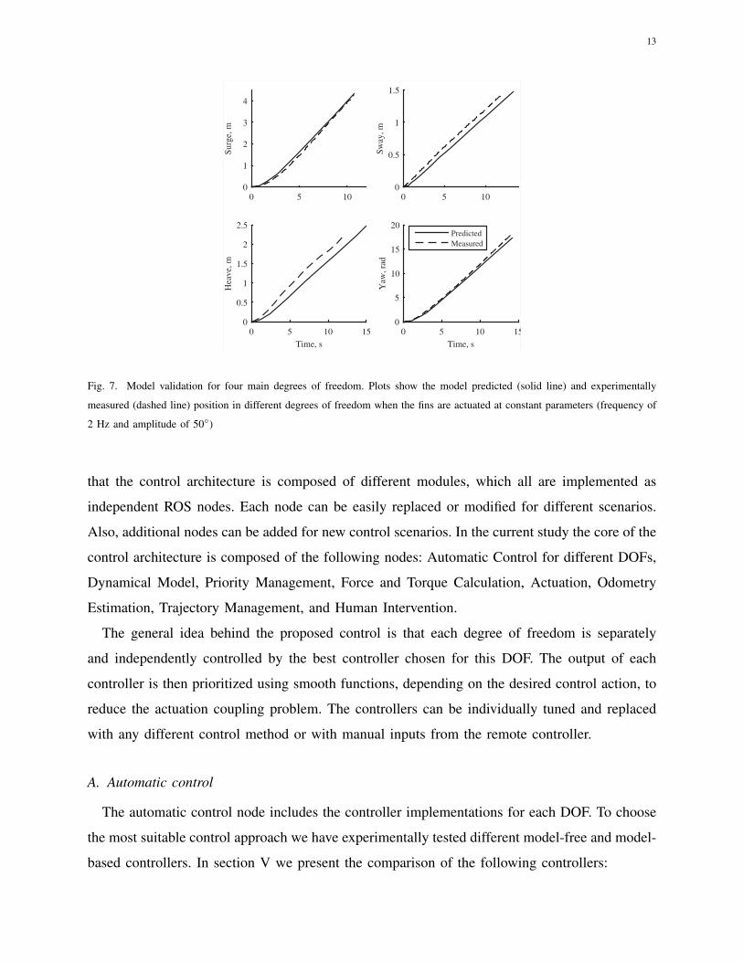
To validate the precision of the model we compared the experimentally measured motion and
the model-predicted motion in each degree of freedom. The obtained results for a single actuation
amplitude and frequency are presented on Fig. 7. It can be seen that the model-predicted position
of the robot matches the actual position with a high precision.
IV. CONTROL ARCHITECTURE
We propose a modular, easily extensible control architecture that allows rapid and simple
controller implementation and testing, but which also can be used during a wide range of
different real mission scenarios (see Fig 8). The control architecture is implemented fully in
general matrix form. Matrix form implementation allows to quickly work with different DOFs
without the need to reimplement any parts of the architecture if additional DOF’s need to be
added to the control. The second feature, which simplifies the testing and implementation, is
13
0 5 10
Surg
e, m
0
1
2
3
4
0 5 10
Sway
, m
0
0.5
1
1.5
Time, s0 5 10 15
Hea
ve, m
0
0.5
1
1.5
2
2.5
Time, s0 5 10 15
Yaw
, rad
0
5
10
15
20PredictedMeasured
Fig. 7. Model validation for four main degrees of freedom. Plots show the model predicted (solid line) and experimentally
measured (dashed line) position in different degrees of freedom when the fins are actuated at constant parameters (frequency of
2 Hz and amplitude of 50◦)
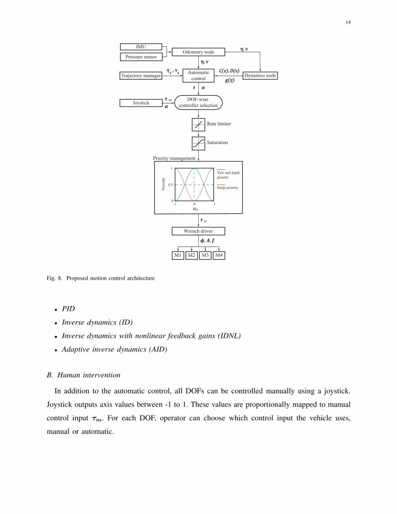
that the control architecture is composed of different modules, which all are implemented as
independent ROS nodes. Each node can be easily replaced or modified for different scenarios.
Also, additional nodes can be added for new control scenarios. In the current study the core of the
control architecture is composed of the following nodes: Automatic Control for different DOFs,
Dynamical Model, Priority Management, Force and Torque Calculation, Actuation, Odometry
Estimation, Trajectory Management, and Human Intervention.
The general idea behind the proposed control is that each degree of freedom is separately
and independently controlled by the best controller chosen for this DOF. The output of each
controller is then prioritized using smooth functions, depending on the desired control action, to
reduce the actuation coupling problem. The controllers can be individually tuned and replaced
with any different control method or with manual inputs from the remote controller.
A. Automatic control
The automatic control node includes the controller implementations for each DOF. To choose
the most suitable control approach we have experimentally tested different model-free and model-
based controllers. In section V we present the comparison of the following controllers:
14
IMU
Pressure sensorOdometry node
Trajectory manager
Wrench driver
𝜂, ν
𝜂 , νd d
𝝉
Saturation
Rate limiter
Priority management
Yaw and depth priority
Surge priority
1-1 0
1
0
0.5
𝛼₁
Prio
rity
𝝉 �𝜶
M1 M2 M3 M4
𝝓, 𝑨, 𝒇
𝝉 �
Joystick
Dynamics nodeAutomaticcontrol
DOF-wise controller selection
𝜶
C(ν), D(ν)
g(𝜂)
𝜂, ν
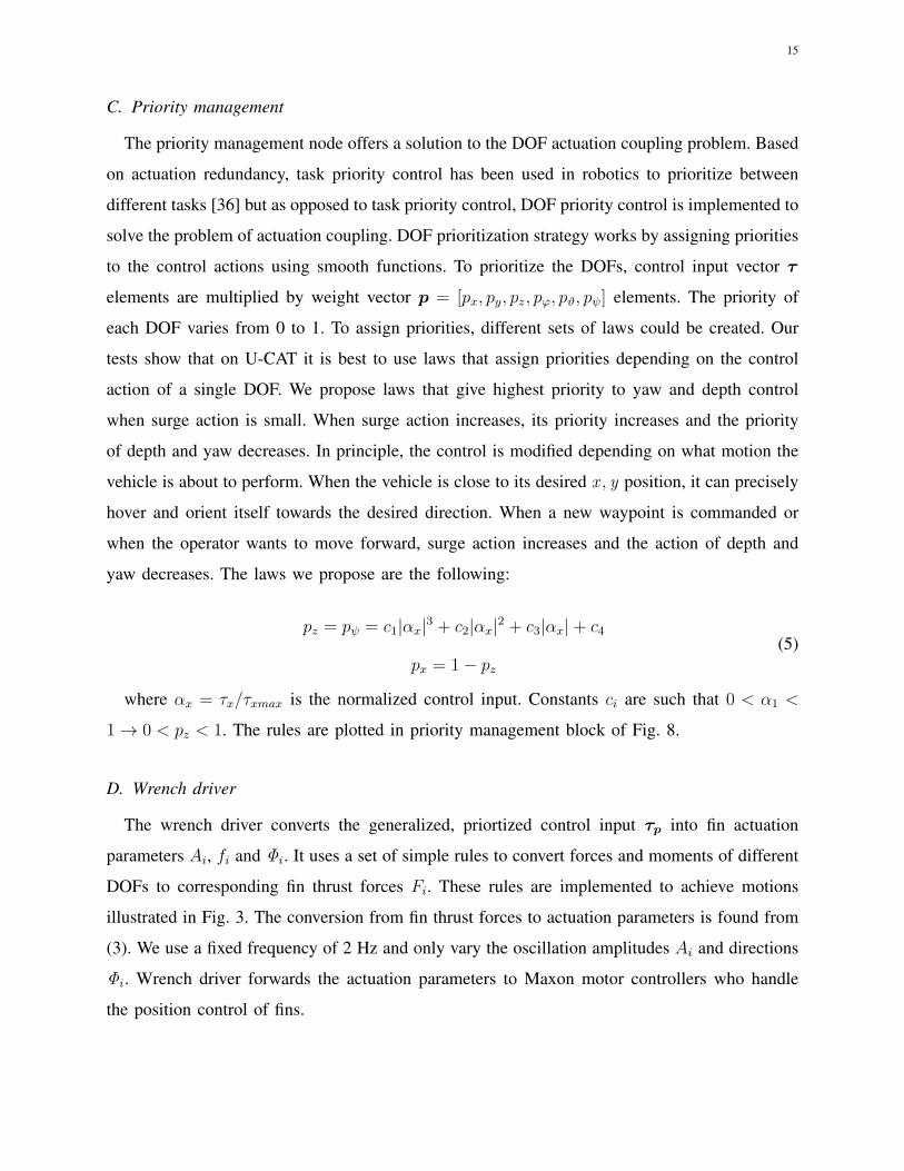
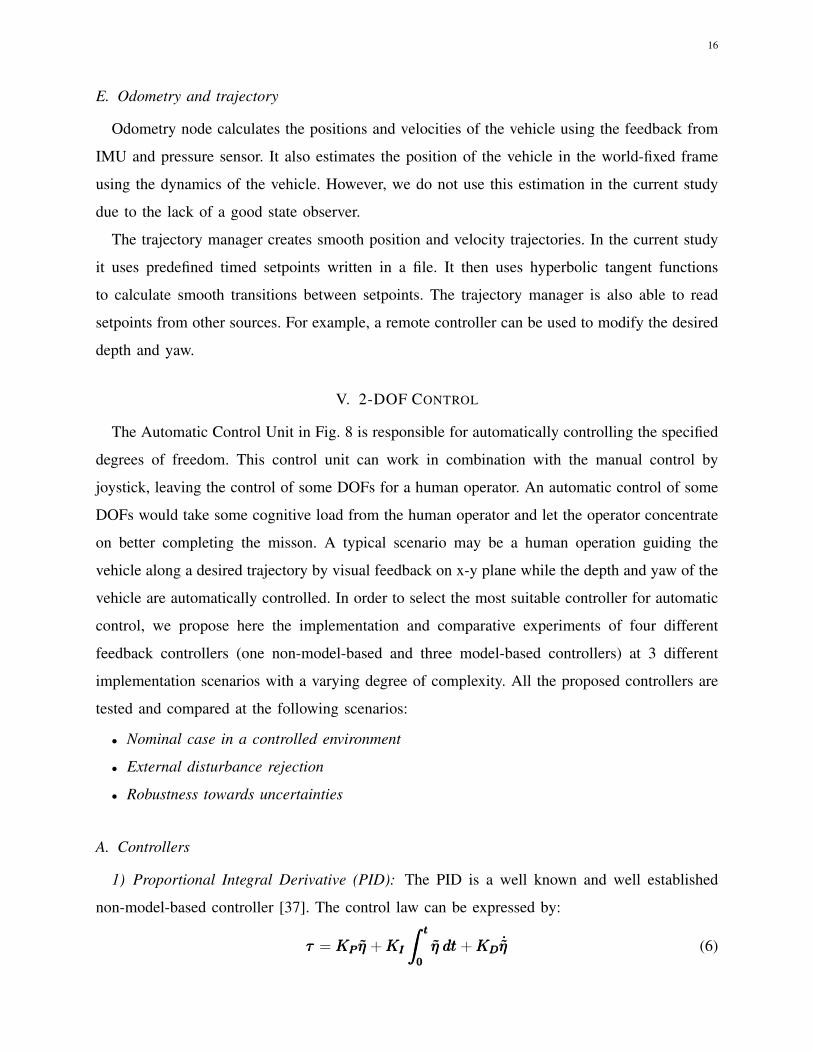
Fig. 8. Proposed motion control architecture
• PID
• Inverse dynamics (ID)
• Inverse dynamics with nonlinear feedback gains (IDNL)
• Adaptive inverse dynamics (AID)
B. Human intervention
In addition to the automatic control, all DOFs can be controlled manually using a joystick.
Joystick outputs axis values between -1 to 1. These values are proportionally mapped to manual
control input τm. For each DOF, operator can choose which control input the vehicle uses,
manual or automatic.
15
C. Priority management
The priority management node offers a solution to the DOF actuation coupling problem. Based
on actuation redundancy, task priority control has been used in robotics to prioritize between
different tasks [36] but as opposed to task priority control, DOF priority control is implemented to
solve the problem of actuation coupling. DOF prioritization strategy works by assigning priorities
to the control actions using smooth functions. To prioritize the DOFs, control input vector τ
elements are multiplied by weight vector p = [px, py, pz, pϕ, pϑ, pψ] elements. The priority of
each DOF varies from 0 to 1. To assign priorities, different sets of laws could be created. Our
tests show that on U-CAT it is best to use laws that assign priorities depending on the control
action of a single DOF. We propose laws that give highest priority to yaw and depth control
when surge action is small. When surge action increases, its priority increases and the priority
of depth and yaw decreases. In principle, the control is modified depending on what motion the
vehicle is about to perform. When the vehicle is close to its desired x , y position, it can precisely
hover and orient itself towards the desired direction. When a new waypoint is commanded or
when the operator wants to move forward, surge action increases and the action of depth and
yaw decreases. The laws we propose are the following:
pz = pψ = c1|αx|3 + c2|αx|2 + c3|αx|+ c4
px = 1− pz(5)
where αx = τx/τxmax is the normalized control input. Constants ci are such that 0 < α1 <
1→ 0 < pz < 1. The rules are plotted in priority management block of Fig. 8.
D. Wrench driver
The wrench driver converts the generalized, priortized control input τp into fin actuation
parameters Ai, fi and Φi . It uses a set of simple rules to convert forces and moments of different
DOFs to corresponding fin thrust forces Fi. These rules are implemented to achieve motions
illustrated in Fig. 3. The conversion from fin thrust forces to actuation parameters is found from
(3). We use a fixed frequency of 2 Hz and only vary the oscillation amplitudes Ai and directions
Φi . Wrench driver forwards the actuation parameters to Maxon motor controllers who handle
the position control of fins.
16
E. Odometry and trajectory
Odometry node calculates the positions and velocities of the vehicle using the feedback from
IMU and pressure sensor. It also estimates the position of the vehicle in the world-fixed frame
using the dynamics of the vehicle. However, we do not use this estimation in the current study
due to the lack of a good state observer.
The trajectory manager creates smooth position and velocity trajectories. In the current study
it uses predefined timed setpoints written in a file. It then uses hyperbolic tangent functions
to calculate smooth transitions between setpoints. The trajectory manager is also able to read
setpoints from other sources. For example, a remote controller can be used to modify the desired
depth and yaw.
V. 2-DOF CONTROL
The Automatic Control Unit in Fig. 8 is responsible for automatically controlling the specified
degrees of freedom. This control unit can work in combination with the manual control by
joystick, leaving the control of some DOFs for a human operator. An automatic control of some
DOFs would take some cognitive load from the human operator and let the operator concentrate
on better completing the misson. A typical scenario may be a human operation guiding the
vehicle along a desired trajectory by visual feedback on x-y plane while the depth and yaw of the
vehicle are automatically controlled. In order to select the most suitable controller for automatic
control, we propose here the implementation and comparative experiments of four different
feedback controllers (one non-model-based and three model-based controllers) at 3 different
implementation scenarios with a varying degree of complexity. All the proposed controllers are
tested and compared at the following scenarios:
• Nominal case in a controlled environment
• External disturbance rejection
• Robustness towards uncertainties
A. Controllers
1) Proportional Integral Derivative (PID): The PID is a well known and well established
non-model-based controller [37]. The control law can be expressed by:
τττ = KP ηKP ηKP η +KI
∫ t
0
ηKI
∫ t
0
ηKI
∫ t
0
η dtdtdt+KD˙ηKD˙ηKD˙η (6)
17
ηηη = ηηη − ηdηdηd is the tracking error, and ˙ηηη is its first time derivative. KPKPKP ,KIKIKI ,KDKDKD are positive
definite matrices representing the proportional, the integral, and the derivative feedback gains
respectively.
2) Inverse dynamics (ID): The main idea of this controller is to fully linearize the dynamics
of the robot based on a nonlinear feedback law to obtain a linear system [33]. Consider the
nonlinear dynamics (1) of the robot, and consider the following nonlinear feedback control law:
τττ = MabMabMab + n(ν, η)n(ν, η)n(ν, η) (7)
with ababab the body frame commanded acceleration, that can be calculated from a simple trans-
formation between the body and the earth fixed-frames as ababab = J−1J−1J−1(ananan − JνJνJν), and ananan =
ηdηdηd −KP ηKP ηKP η −KI
∫ t0ηKI
∫ t0ηKI
∫ t0η dtdtdt −KD
˙ηKD˙ηKD˙η, where ηdηdηd is the desired trajectory and ηdηdηd is its corresponding
acceleration. The control law (7), if replaced in the robot’s dynamics (1), leads to:
(JJJννν + JνJνJν) = ηdηdηd −KP ηKP ηKP η −KI
∫ t
0
ηKI
∫ t
0
ηKI
∫ t
0
η dtdtdt−KD˙ηKD˙ηKD˙η (8)
Now consider the robot’s kinematics (2), its first derivative leads to ηηη = JJJννν + JJJννν, which if
combined with (8) gives:
¨ηηη +KD˙ηKD˙ηKD˙η +KP ηKP ηKP η +KI
∫ t
0
ηKI
∫ t
0
ηKI
∫ t
0
η dtdtdt = 0 (9)
With an appropriate choice of the feedback gains KPKPKP ,KIKIKI ,KDKDKD, the closed-loop dynamics is
asymptotically stable.
3) Inverse dynamics with nonlinear feedback gains (IDNL): This approach has the same
control law as the previous one, except that feedback gains are no longer constants. The use of
nonlinear varying feedback gains may improve the tracking performance of the controller. For
instance, the Nonlinear Computed Torque [38] and the Nonlinear Augmented PD [39] provided
better tracking performance than the conventional computed torque and augmented PD controllers
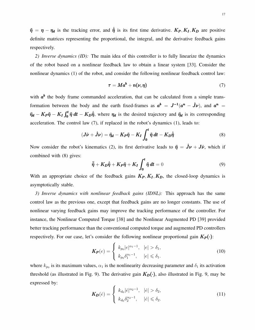
respectively. For our case, let’s consider the following nonlinear proportional gain KP (·)KP (·)KP (·):
KPKPKP (e) =
kp0|e|α1−1, |e| > δ1,
kp0δα1−11 , |e| 6 δ1.
(10)
where kp0 is its maximum values, α1 is the nonlinearity decreasing parameter and δ1 its activation
threshold (as illustrated in Fig. 9). The derivative gain KD(·)KD(·)KD(·), also illustrated in Fig. 9, may be
expressed by:
KDKDKD(e) =
kd0|e|α2−1, |e| > δ2,
kd0δα2−12 , |e| 6 δ2.
(11)
18
0.65kp0
0.7kp0
0.75kp0
0.8kp0
0.85kp0
0.9kp0
0.95kp0
kp0
1.05kp0
0.95kd0
kd0
1.05kd0
1.1kd0
1.15kd0
1.2kd0
1.25kd0
1.3kd0
1.35kd0
−4 −3 −2 −1 0 1 2 3 4
kp0
kd0
kp(e)
kd(e)
Fig. 9. Typical evolution of the nonlinear proportional KP and derivative KD gain versus position error e and velocity error
e (respectively) with α1 = 0.75, δ1 = 1, α2 = 1.25 and δ2 = 1.
with kd0 is its minimum value, α2 is the nonlinearity increasing parameter and δ2 its activation
threshold.
4) Adaptive inverse dynamics (AID): The adaptive inverse dynamics controller is a state
feedback controller with an adaptation control term. It provides an online estimation of possible
unknown model parameters in order to ensure a good trajectory tracking [33]. The control law
can be expressed by:
τττ = MabMabMab + n(ν, η)n(ν, η)n(ν, η) (12)
where the hatted variables denote the dynamics matrices based on estimations, n(ν, η)n(ν, η)n(ν, η) the
estimate of n(ν, η)n(ν, η)n(ν, η) in (7). Since the dynamic model is linear in its parameters, the adaptive
control law (12) can then be rewritten as:
τττ = Φ(ab, ν, η)θΦ(ab, ν, η)θΦ(ab, ν, η)θ (13)
where ΦΦΦ represents the regressor and θθθ is the vector of the online estimated parameters. ababab and
ananan are computed as in the inverse dynamics controller. The vector of estimated parameters is
updated online based on the following adaptive law:
˙θ˙θθ = −ΓΦT (ab, ν, η)J−1yΓΦT (ab, ν, η)J−1yΓΦT (ab, ν, η)J−1y (14)
where the diagonal positive definite matrix ΓΓΓ represents the adaptation gain, JJJ the transformation
matrix, and yyy is the combined tracking error given by yyy = c0ηηη + c1 ˙ηηη. c0 and c1 are positive
constant gains, that may be chosen using the algorithm presented in [33], and based on Barbalat’s
lemma, it ensures that yyy converges to zero.
19
B. Implementation details
The comparative experiments of 2-DOF control have been carried out in the swimming pool
of the University of Montpellier in France with the aim of choosing the most suitable controller
for the automatic control mode of the architecture of Fig. 8. The 2DOF control experiments
where implemented as follows:
• The parameters of each controller are tuned for the nominal case and kept unchanged for
the other scenarios.
• All the proposed controllers were implemented on U-CAT using the ROS based control
architecture presented in section IV
• Two degrees of freedom are to be simultaneously controlled (namely depth and yaw).
• All the relevant real-time data were saved to ROS log files (rosbags). The use of rosbags
enables inspecting the data exactly in the same form as used by the robot software.
Next we will briefly describe all the three implementation scenarios, present the results and
discuss the selection of the 2-DOF controller. The tuned parameters of the proposed controllers
are summarized in Tables I, II, III and IV.
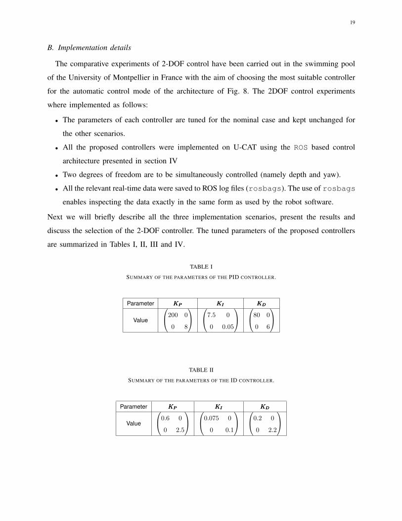
TABLE I
SUMMARY OF THE PARAMETERS OF THE PID CONTROLLER.
Parameter KPKPKP KIKIKI KDKDKD
Value
200 0
0 8
7.5 0
0 0.05
80 0
0 6
TABLE II
SUMMARY OF THE PARAMETERS OF THE ID CONTROLLER.
Parameter KPKPKP KIKIKI KDKDKD
Value
0.6 0
0 2.5
0.075 0
0 0.1
0.2 0
0 2.2
20
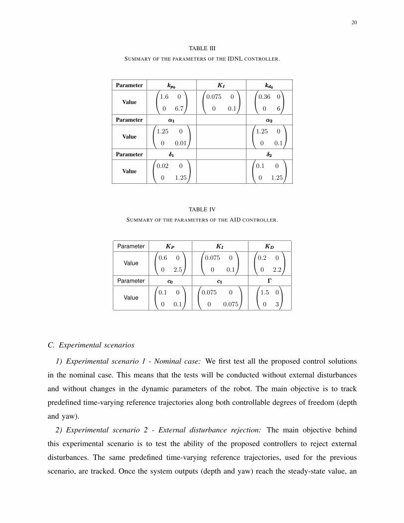
TABLE III
SUMMARY OF THE PARAMETERS OF THE IDNL CONTROLLER.
Parameter kp0kp0kp0 KIKIKI kd0kd0kd0
Value
1.6 0
0 6.7
0.075 0
0 0.1
0.36 0
0 6
Parameter α1α1α1 α2α2α2
Value
1.25 0
0 0.01
1.25 0
0 0.1
Parameter δ1δ1δ1 δ2δ2δ2
Value
0.02 0
0 1.25
0.1 0
0 1.25
TABLE IV
SUMMARY OF THE PARAMETERS OF THE AID CONTROLLER.
Parameter KPKPKP KIKIKI KDKDKD
Value
0.6 0
0 2.5
0.075 0
0 0.1
0.2 0
0 2.2
Parameter c0c0c0 c1c1c1 ΓΓΓ
Value
0.1 0
0 0.1
0.075 0
0 0.075
1.5 0
0 3
C. Experimental scenarios
1) Experimental scenario 1 - Nominal case: We first test all the proposed control solutions
in the nominal case. This means that the tests will be conducted without external disturbances
and without changes in the dynamic parameters of the robot. The main objective is to track
predefined time-varying reference trajectories along both controllable degrees of freedom (depth
and yaw).
2) Experimental scenario 2 - External disturbance rejection: The main objective behind
this experimental scenario is to test the ability of the proposed controllers to reject external
disturbances. The same predefined time-varying reference trajectories, used for the previous
scenario, are tracked. Once the system outputs (depth and yaw) reach the steady-state value, an
21
Fig. 10. View of the robot with increased floatability, a piece of float fixed to the body of the robot increases its buoyancy.
external disturbance is applied, the behaviour of the system is recorded to show the reaction of
the controller and its ability to steer back the system’s outputs to their reference values.
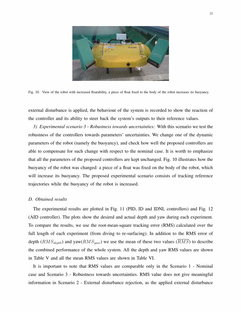
3) Experimental scenario 3 - Robustness towards uncertainties: With this scenario we test the
robustness of the controllers towards parameters’ uncertainties. We change one of the dynamic
parameters of the robot (namely the buoyancy), and check how well the proposed controllers are
able to compensate for such change with respect to the nominal case. It is worth to emphasize
that all the parameters of the proposed controllers are kept unchanged. Fig. 10 illustrates how the
buoyancy of the robot was changed: a piece of a float was fixed on the body of the robot, which
will increase its buoyancy. The proposed experimental scenario consists of tracking reference
trajectories while the buoyancy of the robot is increased.
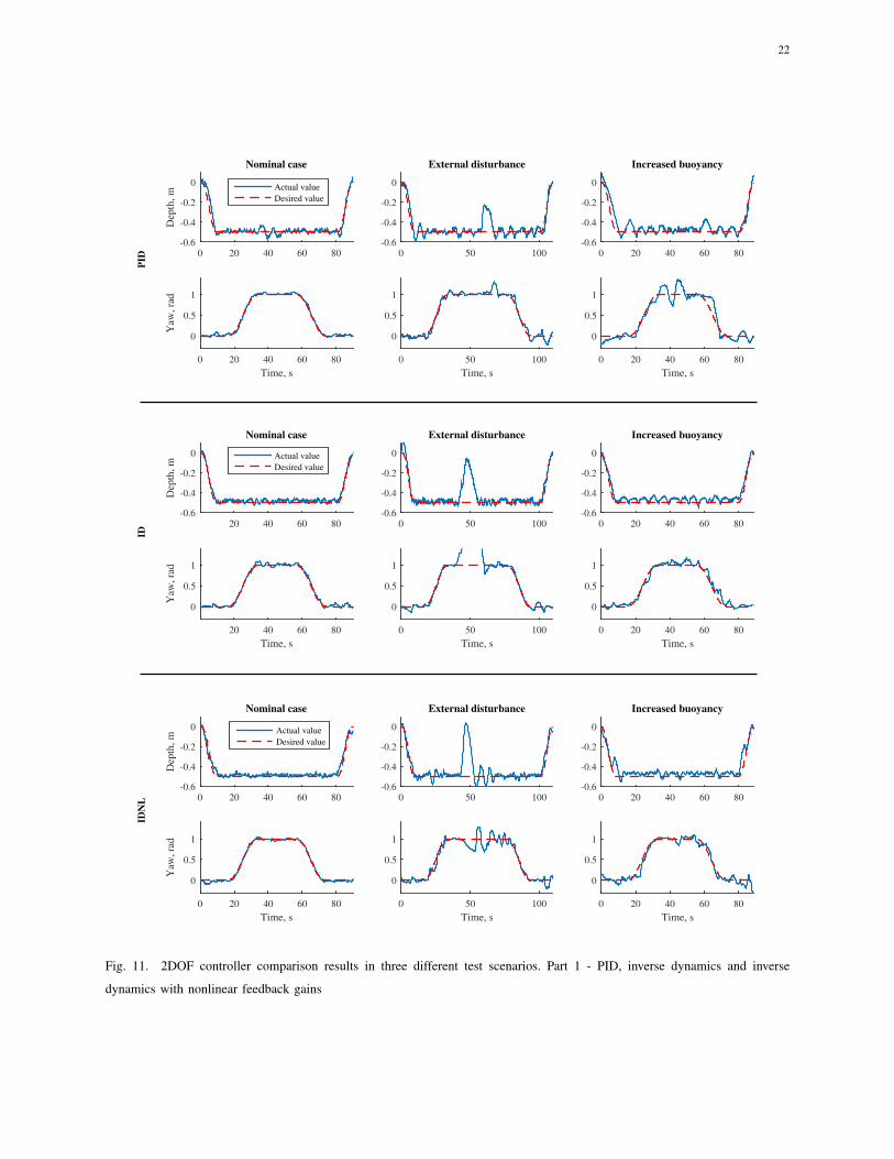
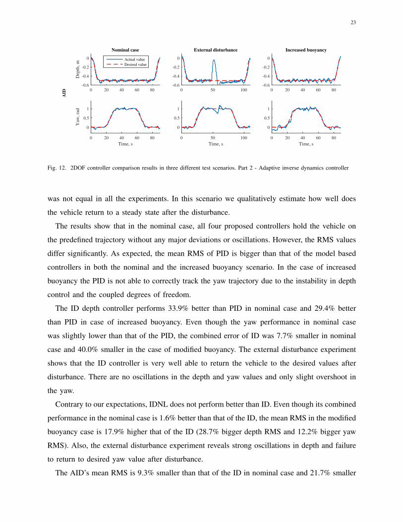
D. Obtained results
The experimental results are plotted in Fig. 11 (PID, ID and IDNL controllers) and Fig. 12
(AID controller). The plots show the desired and actual depth and yaw during each experiment.
To compare the results, we use the root-mean-square tracking error (RMS) calculated over the
full length of each experiment (from diving to re-surfacing). In addition to the RMS error of
depth (RMSdepth) and yaw(RMSyaw) we use the mean of these two values (RMS) to describe
the combined performance of the whole system. All the depth and yaw RMS values are shown
in Table V and all the mean RMS values are shown in Table VI.
It is important to note that RMS values are comparable only in the Scenario 1 - Nominal
case and Scenario 3 - Robustness towards uncertainties. RMS value does not give meaningful
information in Scenario 2 - External disturbance rejection, as the applied external disturbance
22
0 20 40 60 80
Dep
th, m
-0.6
-0.4
-0.2
0
Nominal case
Time, s0 20 40 60 80
Yaw
, rad
0
0.5
1
0 50 100-0.6
-0.4
-0.2
0
External disturbance
Time, s0 50 100
0
0.5
1
0 20 40 60 80-0.6
-0.4
-0.2
0
Increased buoyancy
Actual valueDesired value
Time, s0 20 40 60 80
0
0.5
1
20 40 60 80
Dep
th, m
-0.6
-0.4
-0.2
0
Nominal case
Time, s20 40 60 80
Yaw
, rad
0
0.5
1
0 50 100-0.6
-0.4
-0.2
0
External disturbance
Time, s0 50 100
0
0.5
1
0 20 40 60 80-0.6
-0.4
-0.2
0
Increased buoyancy
Actual valueDesired value
Time, s0 20 40 60 80
0
0.5
1
0 20 40 60 80
Dep
th, m
-0.6
-0.4
-0.2
0
Nominal case
Time, s0 20 40 60 80
Yaw
, rad
0
0.5
1
0 50 100-0.6
-0.4
-0.2
0
External disturbance
Time, s0 50 100
0
0.5
1
0 20 40 60 80-0.6
-0.4
-0.2
0
Increased buoyancy
Actual valueDesired value
Time, s0 20 40 60 80
0
0.5
1
PID
IDID
NL
Fig. 11. 2DOF controller comparison results in three different test scenarios. Part 1 - PID, inverse dynamics and inverse
dynamics with nonlinear feedback gains
23
0 20 40 60 80
Dep
th, m
-0.6
-0.4
-0.2
0
Nominal case
Time, s0 20 40 60 80
Yaw
, rad
0
0.5
1
0 50 100-0.6
-0.4
-0.2
0
External disturbance
Time, s0 50 100
0
0.5
1
0 20 40 60 80-0.6
-0.4
-0.2
0
Increased buoyancy
Actual valueDesired value
Time, s0 20 40 60 80
0
0.5
1
AID
Fig. 12. 2DOF controller comparison results in three different test scenarios. Part 2 - Adaptive inverse dynamics controller
was not equal in all the experiments. In this scenario we qualitatively estimate how well does
the vehicle return to a steady state after the disturbance.
The results show that in the nominal case, all four proposed controllers hold the vehicle on
the predefined trajectory without any major deviations or oscillations. However, the RMS values
differ significantly. As expected, the mean RMS of PID is bigger than that of the model based
controllers in both the nominal and the increased buoyancy scenario. In the case of increased
buoyancy the PID is not able to correctly track the yaw trajectory due to the instability in depth
control and the coupled degrees of freedom.
The ID depth controller performs 33.9% better than PID in nominal case and 29.4% better
than PID in case of increased buoyancy. Even though the yaw performance in nominal case
was slightly lower than that of the PID, the combined error of ID was 7.7% smaller in nominal
case and 40.0% smaller in the case of modified buoyancy. The external disturbance experiment
shows that the ID controller is very well able to return the vehicle to the desired values after
disturbance. There are no oscillations in the depth and yaw values and only slight overshoot in
the yaw.
Contrary to our expectations, IDNL does not perform better than ID. Even though its combined
performance in the nominal case is 1.6% better than that of the ID, the mean RMS in the modified
buoyancy case is 17.9% higher that of the ID (28.7% bigger depth RMS and 12.2% bigger yaw
RMS). Also, the external disturbance experiment reveals strong oscillations in depth and failure
to return to desired yaw value after disturbance.
The AID’s mean RMS is 9.3% smaller than that of the ID in nominal case and 21.7% smaller
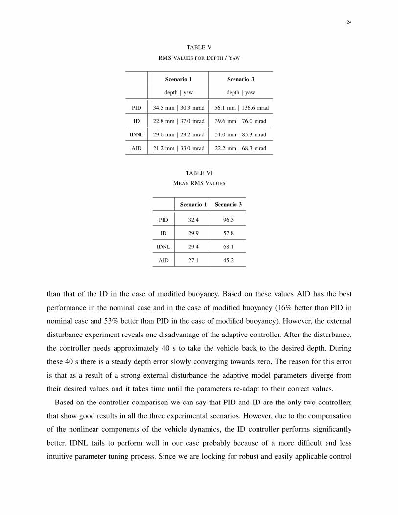
24
TABLE V
RMS VALUES FOR DEPTH / YAW
Scenario 1 Scenario 3
depth | yaw depth | yaw
PID 34.5 mm | 30.3 mrad 56.1 mm | 136.6 mrad
ID 22.8 mm | 37.0 mrad 39.6 mm | 76.0 mrad
IDNL 29.6 mm | 29.2 mrad 51.0 mm | 85.3 mrad
AID 21.2 mm | 33.0 mrad 22.2 mm | 68.3 mrad
TABLE VI
MEAN RMS VALUES
Scenario 1 Scenario 3
PID 32.4 96.3
ID 29.9 57.8
IDNL 29.4 68.1
AID 27.1 45.2
than that of the ID in the case of modified buoyancy. Based on these values AID has the best
performance in the nominal case and in the case of modified buoyancy (16% better than PID in
nominal case and 53% better than PID in the case of modified buoyancy). However, the external
disturbance experiment reveals one disadvantage of the adaptive controller. After the disturbance,
the controller needs approximately 40 s to take the vehicle back to the desired depth. During
these 40 s there is a steady depth error slowly converging towards zero. The reason for this error
is that as a result of a strong external disturbance the adaptive model parameters diverge from
their desired values and it takes time until the parameters re-adapt to their correct values.
Based on the controller comparison we can say that PID and ID are the only two controllers
that show good results in all the three experimental scenarios. However, due to the compensation
of the nonlinear components of the vehicle dynamics, the ID controller performs significantly
better. IDNL fails to perform well in our case probably because of a more difficult and less
intuitive parameter tuning process. Since we are looking for robust and easily applicable control
25
methods, IDNL is not the best approach. As expected, AID performs significantly better than any
other controller in the test of robustness towards model uncertainties. Therefore, this controller
would be the best choice for missions where the vehicle dynamics changes during the operation.
This includes for example the case where the robot is operated on a long tether that affects the
vehicle’s dynamics. However, AID is not appropriate for missions in which the vehicle may be
exposed to strong external disturbances, such as collision with underwater objects. Our control
architecture allows seamless switching between different control approaches even during the
mission. Either ID or AID can be chosen by the operator depending on the situation.
VI. 3-DOF CONTROL
This section experimentally validates the proposed control architecture with DOF prioritization
for 3D motion of the robot. We describe 5 control strategies where some of the degrees are
controlled by the operator with the joystick and others automatically while using the DOF
priority manager illustrated in Fig. 8. These tests are also compared to the scenario where the
DOF priority management is switched off.
The experiments were conducted in a 60 m long, 5 m wide and 3 m deep fresh water tow
tank of Tallinn University of Technology. In all the experiments the robot followed a lawnmower
trajectory at constant depth of 1 m. Each experiment started with a dive and ended with a
resurface. We chose the lawnmower trajectory because of its wide use in underwater inspection
tasks. During the experiments the robot recorded its depth and yaw data into ROS log files.
As the acoustic positioning methods did not work in a concrete tank, we did not have any
real-time position feedback for translational motions on the horizontal plane. However, we used
a calibrated overhead camera for recording the vehicle trajectories. After the experiments we
manually tracked the position of U-CAT from the overhead video frame by frame.
A. Experimental scenarios
We tested the following 5 control approaches:
1) Fully manual control: An experienced U-CAT operator controlled depth, yaw and surge
to follow the predefined trajectory as precisely as possible while keeping constant depth. In this
scenario the automatic control unit on Fig. 8 is switched off and the commands from the joystick
are processed by the priority manager. The operator used visual feedback and a depth reading
on screen. The lawnmower trajectory was relatively loosely defined in our experiments, as there
26
was no precise position feedback other than visual. The operator used markers on the poolside
to approximately travel a same distance with every short leg of the trajectory. For comparative
reasons the operator also tried to follow the same trajectory timing as in other experiments.
2) Depth autopilot: In this experiment the automatic control unit in Fig. 8 controls only depth
while the operator controlled other DOFs (yaw and surge) manually.
3) Depth and yaw autopilot: In this experiment the operator’s manual control was kept
minimal as he only controlled the surge motion with the joystick to move the vehicle from
one turning point to another while depth and yaw motion where controlled automatically.
4) Fully autonomous control: As U-CAT is designed to eventually be fully autonomous, we
also tested the extensibility of our control approach to fully autonomous control mode. In this
case the vehicle was untethered and the operator was removed from the control loop. The manual
surge regulation was replaced by automatic open-loop control. As we did not have any surge
velocity or position feedback, the surge control was implemented as a smooth predefined force
trajectory.
5) Fully autonomous control without DOF prioritization: In this experiment we repeated the
fully autonomous control scenario, but we disabled the priority manager. All 3 DOF (depth,
yaw and surge) where controlled by the Autonomous control unit in Fig. 8 while the Priority
Manager was turned off.
B. Obtained Results
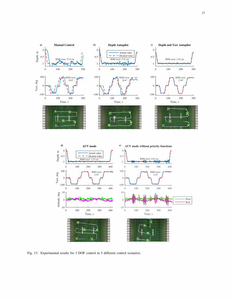
The desired and actual trajectories for each of the above experiments are shown in Fig. 13.
Root mean square (RMS) error values calculated over the full length of experiments are marked
on the graphs.
1) Manual Control: Fig. 13a shows the desired and actual trajectories of depth, yaw, x and
y. From the figure it can be easily seen that the trajectory following precision is poor (depth
RMS error of 27.6 cm and yaw RMS error of 39.8◦). This illustrates the definite need for at
least some autopiloting.
2) Depth Autopilot: In this experiment the depth autopilot was enabled while the operator
manually controlled the surge and yaw. Results show 81% decrease in depth error compared to
the manual control. In addition yaw error decreased 28% as now the operator had to concentrate
on controlling only 2 DOFs instead of 3. However, the overhead camera image still reveals the
lack of precision in tracking straight lines. The vehicle turns rapidly. This kind of unsteady motion
27
0 100 200 300 400
Dep
th, m
-1
-0.5
0
AUV mode
Actual valueDesired value
0 100 200 300 400
Yaw
, deg
-100
0
100
Time, s0 100 200 300 400
Atti
tude
, deg
-10
0
10
0 100 200 300
-1
-0.5
0
Depth and Yaw Autopilot
Time, s0 100 200 300
-100
0
100
0 100 200 300
Dep
th, m
-1
-0.5
0
Manual Control
Time, s0 100 200 300
Yaw
, deg
-100
0
100
0 100 200 300
-1
-0.5
0
Depth Autopilot
Actual valueDesired value
Time, s0 100 200 300
-100
0
100
0 100 200 300 400
-1
-0.5
0
AUV mode without priority functions
0 100 200 300 400-100
0
100
Time, s0 100 200 300 400
-10
0
10
PitchRoll
d) e)
a) b) c)
RMS error: 27.6 cm RMS error: 5.22 cm RMS error: 1.93 cm
RMS error: 2.22 cm RMS error: 4.62 cm
RMS error:39.8º
RMS error:28.6º
RMS error:2.50º
RMS error2.91º
RMS error:3.23º
Fig. 13. Experimental results for 3 DOF control in 5 different control scenarios.
28
would probably cause problems in video inspection tasks, especially when using automatic video
processing methods such as mosaicking.
3) Depth and Yaw Autopilot: In this experiment we also enabled automatic yaw control.
This time the operator intervention was minimal. He only had to control the surge motion
to move the vehicle from one turning point to another. The obtained results (Fig. 13c) show
high precision in yaw tracking (RMS error of 2.5◦ ; improvement of 91%). Also, due to more
steady yaw the depth tracking error decreased by 63% compared to the scenario with only
depth autopilot. More stable yaw is also visible from the overhead camera image. It shows
how the robot moves in straight lines between turning points. Unfortunately, the short legs of
the trajectory (vertical on the overhead camera images) are not perpendicular to the long legs.
This is caused by the disturbance of the tether, which slowly pulled the vehicle sideways. The
disturbances are inevitable and during ROV missions they have to be manually compensated for.
The compensation can be relatively easily done as the U-CAT’s fins also allow to actuate the
sway motion to move the vehicle sideways. In this article, however, we do not consider sway
control.
4) Fully Autonomous Control: The results depicted in Fig. 13d show that removing human
intervention did not significantly reduce the tracking precision. Also, the tether disturbance is
not any more visible on the overhead image. However, the figure reveals an IMU drift in yaw
signal which was not present in our previous experiments. We have noticed that large IMU drift
sometimes occurs due to electromagnetic noise emitted by the motor controllers. The drift is
small enough (0.9 deg/min) to not affect the controller behaviour. For real missions the drift
will be reduced by minimizing electromagnetic noise and by using magnetometers and Extended
Kalman Filter. Despite the IMU issue the experiment shows that our control approach is suitable
for simultaneously controlling 3 DOFs of the fully autonomous 4-fin vehicle. Once the vehicle
has a reliable position or surge velocity estimation, the current surge controller can be replaced
by a suitable closed-loop controller.
5) Fully autonomous control without DOF prioritization: The test results without the priority
manager in Fig. 13 e show strong oscillations of depth value. The oscillations occur when the
surge action increases and the vehicle tries to move forward. The figure also displays the roll
and pitch angles in comparison to those during the previous experiment (Fig. 13 d). It can be
seen that the vehicle is strongly oscillating in pitch and roll. The oscillations are the result of a
coupling between the actuation of different DOFs. All the controllers try to stabilize the vehicle,
29
however the fin configuration does not allow to equally control all the DOFs at the same time.
The resulting lawnmower trajectory is also different from that of the experiment 4 as the vehicle
can not correctly output the predefined surge force. These results clearly show the importance
of DOF prioritization in our system.
VII. VALIDATION IN NATURAL ENVIRONMENT
This section describes two real-life test scenarios in natural environments where the control
of the robot was validated during a real mission.
A. ROV Inspection Missions of Submerged Machinery
The first testsite is located in Rummu quarry in Estonia (59◦13’35.8”N 24◦13’30.48”E).
Rummu quarry is an abandoned flooded limestone mine containing submerged building and
several large mining machines. We inspected a mining excavator in 11m depth with the U-CAT
in an ROV mode. Two missions where carried out on this test site in different environmental
conditions:
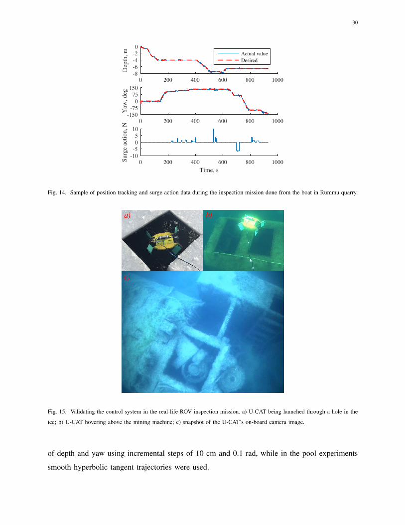
• 1 - Winter experiment (3rd of March 2016) - we launched the vehicle through an 1x1 meter
hole (see Fig. 15a) cut into 20 cm thick layer of ice.
• 2 - Summer experiment (14th of July 2016) - we launched the vehicle from a small (4.3
m) rowboat.
During the mission the depth and yaw were autopiloted by the inverse dynamics controller.
The operator used a joystick to modify the controller setpoints and to manually control the surge
speed of the vehicle. He used the live video feedback (Fig. 15c) from the downward looking
on-board camera to inspect the different parts of the machine.
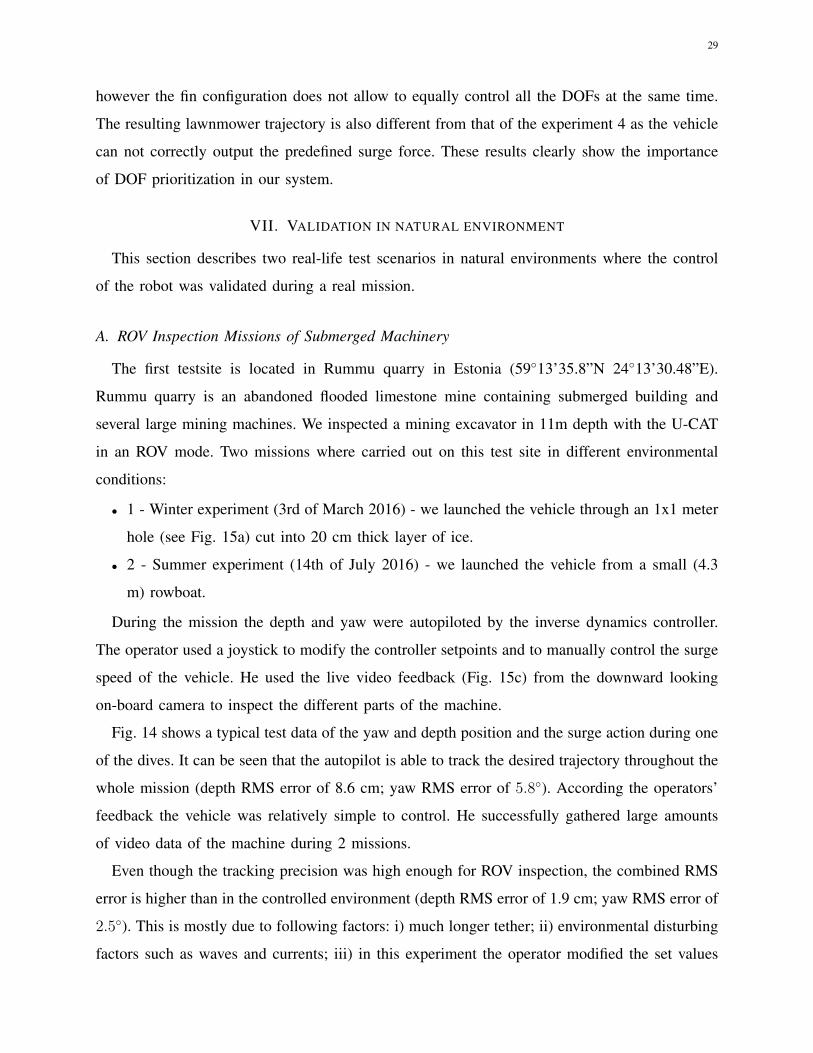
Fig. 14 shows a typical test data of the yaw and depth position and the surge action during one
of the dives. It can be seen that the autopilot is able to track the desired trajectory throughout the
whole mission (depth RMS error of 8.6 cm; yaw RMS error of 5.8◦). According the operators’
feedback the vehicle was relatively simple to control. He successfully gathered large amounts
of video data of the machine during 2 missions.
Even though the tracking precision was high enough for ROV inspection, the combined RMS
error is higher than in the controlled environment (depth RMS error of 1.9 cm; yaw RMS error of
2.5◦). This is mostly due to following factors: i) much longer tether; ii) environmental disturbing
factors such as waves and currents; iii) in this experiment the operator modified the set values
30
0 200 400 600 800 1000
Dep
th, m
-8-6-4-20
Actual valueDesired
0 200 400 600 800 1000Y
aw, d
eg
-150-75
075
150
Time, s0 200 400 600 800 1000Su
rge
actio
n, N
-10-505
10
Fig. 14. Sample of position tracking and surge action data during the inspection mission done from the boat in Rummu quarry.
Fig. 15. Validating the control system in the real-life ROV inspection mission. a) U-CAT being launched through a hole in the
ice; b) U-CAT hovering above the mining machine; c) snapshot of the U-CAT’s on-board camera image.
of depth and yaw using incremental steps of 10 cm and 0.1 rad, while in the pool experiments
smooth hyperbolic tangent trajectories were used.
31
0 200 400 600 800
Dep
th, m
-10-8-6-4-20
Actual valueDesired
0 200 400 600 800Y
aw, d
eg
-150-75
075
150
Time, s0 200 400 600 800Su
rge
actio
n, N
-10-505
10
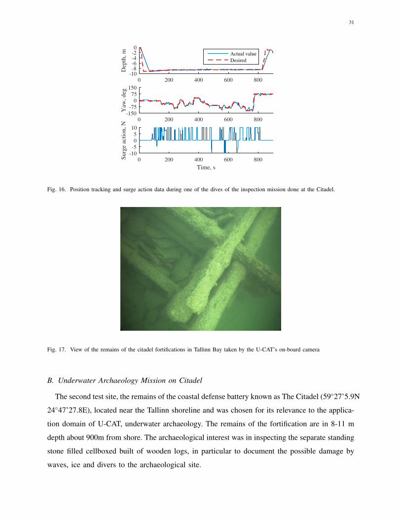
Fig. 16. Position tracking and surge action data during one of the dives of the inspection mission done at the Citadel.
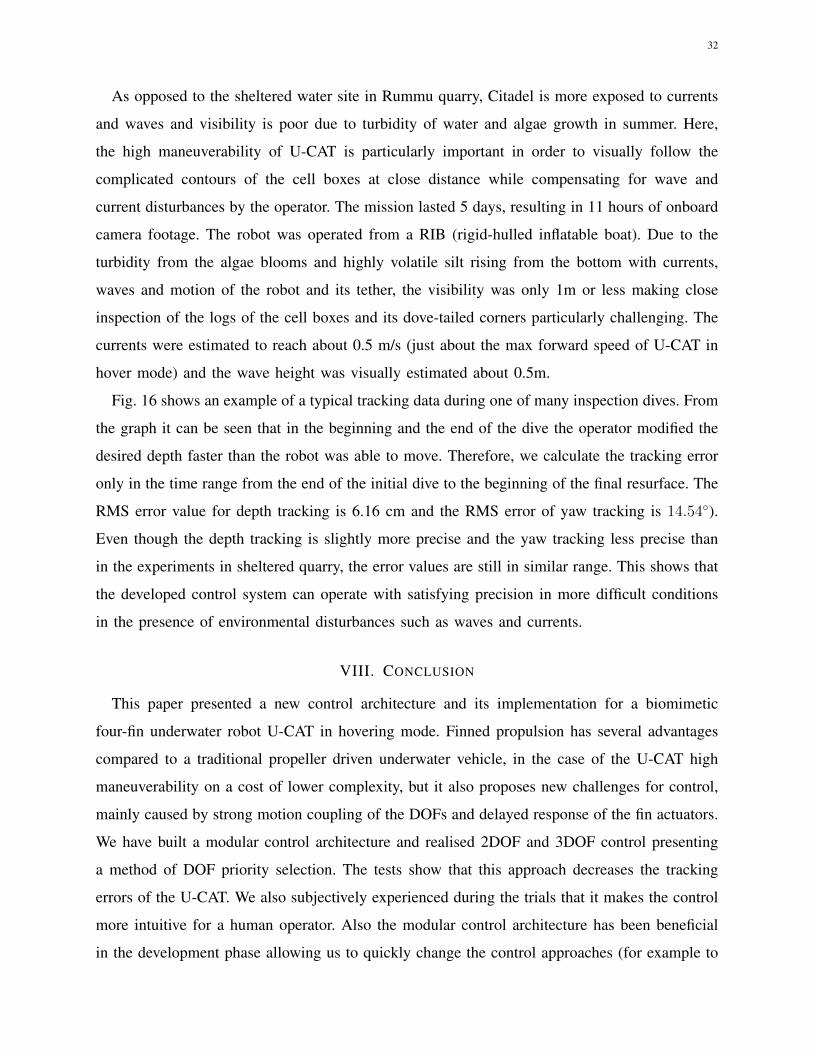
Fig. 17. View of the remains of the citadel fortifications in Tallinn Bay taken by the U-CAT’s on-board camera
B. Underwater Archaeology Mission on Citadel
The second test site, the remains of the coastal defense battery known as The Citadel (59◦27’5.9N
24◦47’27.8E), located near the Tallinn shoreline and was chosen for its relevance to the applica-
tion domain of U-CAT, underwater archaeology. The remains of the fortification are in 8-11 m
depth about 900m from shore. The archaeological interest was in inspecting the separate standing
stone filled cellboxed built of wooden logs, in particular to document the possible damage by
waves, ice and divers to the archaeological site.
32
As opposed to the sheltered water site in Rummu quarry, Citadel is more exposed to currents
and waves and visibility is poor due to turbidity of water and algae growth in summer. Here,
the high maneuverability of U-CAT is particularly important in order to visually follow the
complicated contours of the cell boxes at close distance while compensating for wave and
current disturbances by the operator. The mission lasted 5 days, resulting in 11 hours of onboard
camera footage. The robot was operated from a RIB (rigid-hulled inflatable boat). Due to the
turbidity from the algae blooms and highly volatile silt rising from the bottom with currents,
waves and motion of the robot and its tether, the visibility was only 1m or less making close
inspection of the logs of the cell boxes and its dove-tailed corners particularly challenging. The
currents were estimated to reach about 0.5 m/s (just about the max forward speed of U-CAT in
hover mode) and the wave height was visually estimated about 0.5m.
Fig. 16 shows an example of a typical tracking data during one of many inspection dives. From
the graph it can be seen that in the beginning and the end of the dive the operator modified the
desired depth faster than the robot was able to move. Therefore, we calculate the tracking error
only in the time range from the end of the initial dive to the beginning of the final resurface. The
RMS error value for depth tracking is 6.16 cm and the RMS error of yaw tracking is 14.54◦).
Even though the depth tracking is slightly more precise and the yaw tracking less precise than
in the experiments in sheltered quarry, the error values are still in similar range. This shows that
the developed control system can operate with satisfying precision in more difficult conditions
in the presence of environmental disturbances such as waves and currents.
VIII. CONCLUSION
This paper presented a new control architecture and its implementation for a biomimetic
four-fin underwater robot U-CAT in hovering mode. Finned propulsion has several advantages
compared to a traditional propeller driven underwater vehicle, in the case of the U-CAT high
maneuverability on a cost of lower complexity, but it also proposes new challenges for control,
mainly caused by strong motion coupling of the DOFs and delayed response of the fin actuators.
We have built a modular control architecture and realised 2DOF and 3DOF control presenting
a method of DOF priority selection. The tests show that this approach decreases the tracking
errors of the U-CAT. We also subjectively experienced during the trials that it makes the control
more intuitive for a human operator. Also the modular control architecture has been beneficial
in the development phase allowing us to quickly change the control approaches (for example to
33
switch between different 2DOF controllers). We therefore conclude that the architecture makes
the robot easier to operate both in development phase as well as during real missions. The
tests where carried out in controlled underwater environment, in sheltered water and in open
water environment with waves, currents and very low visibility at a difficult inspection task. The
tracking error increases when moving to more complicated environments, which is expected with
any control approach. However, the control of the robot was sufficiently easy and precise even
during a long real mission in a highly unstable environment. We therefore conclude that the
proposed control architecture is suitable for U-CAT. Our future goal is to extend the control to
more DOFs as well as to extend the motion library of U-CAT to include cruising mode. Again,
we expect the modular control architecture to be beneficial in development and testing phase as
well as on real underwater missions.
ACKNOWLEDGMENT
This research has received funding from the European Unions Seventh Framework Programme
for Research technological development and demonstration, under grant agreement no. 308724
(The ARROWS Project), from Estonian- French joint collaboration project PHC-PARROT and
from IUT339 grant of Estonian Ministry of Education and Research. The authors would like
to thank Keijo Kuusmik, Jaan Rebane, Riho Markna who have helped to develop the UCAT
vehicle. We would also like to thank TUT Small Craft Competence Centre for letting us use the
tow tank.
REFERENCES
[1] B. Anderson and J. Crowell, “Workhorse auv-a cost-sensible new autonomous underwater vehicle for surveys/soundings,
search & rescue, and research,” in OCEANS, 2005. Proceedings of MTS/IEEE. Washington, USA: IEEE, Sep. 2005, pp.
1–6.
[2] (2016) Bluefin robotics website. [Online]. Available: http://www.bluefinrobotics.com/
[3] C. von Alt, “Remus 100 transportable mine countermeasure package,” in OCEANS 2003. Proceedings, vol. 4. San Diego,
USA: IEEE, 2003, pp. 1925–1930.
[4] A. Shukla and H. Karki, “Application of robotics in offshore oil and gas industry a review part
{II},” Robotics and Autonomous Systems, vol. 75, Part B, pp. 508 – 524, 2016. [Online]. Available:
http://www.sciencedirect.com/science/article/pii/S0921889015002018
[5] V. Yordanova and H. Griffiths, “Rendezvous point technique for multivehicle mine countermeasure operations in
communication-constrained environments,” Marine Technology Society Journal, vol. 50, no. 2, pp. 5–16, 2016.
[6] B. Bingham, B. Foley, H. Singh, R. Camilli, K. Delaporta, R. Eustice, A. Mallios, D. Mindell, C. Roman, and D. Sakellariou,
“Robotic tools for deep water archaeology: Surveying an ancient shipwreck with an autonomous underwater vehicle,”
Journal of Field Robotics, vol. 27, no. 6, pp. 702–717, 2010.
34
[7] Y.-S. Ryuh, G.-H. Yang, J. Liu, and H. Hu, “A school of robotic fish for mariculture monitoring in the sea coast,” Journal
of Bionic Engineering, vol. 12, no. 1, pp. 37–46, 2015.
[8] A. Kohl, K. Pettersen, E. Kelasidi, and J. Gravdahl, “Planar path following of underwater snake robots in the presence of
ocean currents,” Robotics and Automation Letters, IEEE, vol. PP, no. 99, pp. 1–1, 2016.
[9] R. J. Lock, R. Vaidyanathan, S. C. Burgess, and J. Loveless, “Development of a biologically inspired multi-modal wing
model for aerial-aquatic robotic vehicles through empirical and numerical modelling of the common guillemot, uria aalge,”
Bioinspiration & biomimetics, vol. 5, no. 4, p. 046001, 2010.
[10] M. Kemp, B. Hobson, and J. H. Long, “Madeleine: an agile auv propelled by flexible fins,” in Proceedings of the 14th
International Symposium on Unmanned Untethered Submersible Technology, vol. 6, 2005.
[11] S. Licht and N. Durham, “Biomimetic robots for environmental monitoring in the surf zone & in very shallow water,” in
IEEE/RSJ International Conference on Intelligent Robots and Systems, Vilamoura-Algarve, Portugal, Oct. 2012.
[12] G. Yao, J. Liang, T. Wang, X. Yang, Q. Shen, Y. Zhang, H. Wu, and W. Tian, “Development of a turtle-like underwater
vehicle using central pattern generator,” in Robotics and Biomimetics (ROBIO), 2013 IEEE International Conference on.
Shenzhen, China: IEEE, Dec. 2013, pp. 44–49.
[13] G. Dudek, P. Giguere, J. Zacher, E. Milios, H. Liu, P. Zhang, M. Buehler, C. Georgiades, C. Prahacs, S. Saunderson et al.,
“Aqua: An amphibious autonomous robot,” Computer, no. 1, pp. 46–53, 2007.
[14] A. Konno, T. Furuya, A. Mizuno, K. Hishinuma, K. Hirata, and M. Kawada, “Development of turtle-like submergence
vehicle,” in Proceedings of the 7th International Symposium on Marine Engineering, 2005.
[15] K. Low, C. Zhou, T. Ong, and J. Yu, “Modular design and initial gait study of an amphibian robotic turtle,” in Robotics
and Biomimetics, 2007. ROBIO 2007. IEEE International Conference on. Sanya, China: IEEE, Dec. 2007, pp. 535–540.
[16] S. C. Licht, “Biomimetic oscillating foil propulsion to enhance underwater vehicle agility and maneuverability,” Ph.D.
dissertation, Massachusetts Institute of Technology, Cambridge, Massachusetts, June 2008.
[17] J. D. Geder, R. Ramamurti, D. Edwards, T. Young, and M. Pruessner, “Development of a robotic fin for hydrodynamic
propulsion and aerodynamic control,” in Oceans-St. John’s, 2014. IEEE, 2014, pp. 1–7.
[18] W. Zhao, Y. Hu, L. Wang, and Y. Jia, “Development of a flipper propelled turtle-like underwater robot and its cpg-based
control algorithm,” in Decision and Control, 2008. CDC 2008. 47th IEEE Conference on. Cancun, Mexico: IEEE, Dec.
2008, pp. 5226–5231.
[19] C. Siegenthaler, C. Pradalier, F. Gunther, G. Hitz, and R. Siegwart, “System integration and fin trajectory design for a
robotic sea-turtle,” in Intelligent Robots and Systems (IROS), 2013 IEEE/RSJ International Conference on. Tokyo, Japan:
IEEE, Nov. 2013, pp. 3790–3795.
[20] J. D. Geder, R. Ramamurti, M. Pruessner, and J. Palmisano, “Maneuvering performance of a four-fin bio-inspired uuv,”
in Oceans-San Diego, 2013. IEEE, 2013.
[21] C. Wang, G. Xie, X. Yin, L. Li, and L. Wang, “Cpg-based locomotion control of a quadruped amphibious robot,” in
Advanced Intelligent Mechatronics (AIM), 2012 IEEE/ASME International Conference on. IEEE, 2012.
[22] A. Chemori, K. Kuusmik, T. Salumae, and M. Kruusmaa, “Depth control of the biomimetic u-cat turtle-like auv with
experiments in real operating conditions,” in Robotics and Automation (ICRA), 2016 IEEE International Conference on.
Stockholm, Sweden: IEEE, May 2016, pp. 1–6.
[23] T. Salumae, A. Chemori, and M. Kruusmaa, “Motion control architecture of a 4-fin u-cat auv using dof prioritization,” in
Intelligent Robots and Systems (IROS), 2016 IEEE/RSJ International Conference on. Daejeon, Korea: IEEE, Oct. 2016.
[24] J. Wyneken, “Sea turtle locomotion: mechanisms, behavior, and energetics,” in The biology of sea turtles, P. L. Lutz and
J. A. Musick, Eds. Boca Raton, FL: CRC Press, 1997, ch. 7, pp. 165–198.
35
[25] S.-H. Song, M.-S. Kim, H. Rodrigue, J.-Y. Lee, J.-E. Shim, M.-C. Kim, W.-S. Chu, and S.-H. Ahn, “Turtle mimetic soft
robot with two swimming gaits,” Bioinspiration I& Biomimetics, vol. 11, no. 3, p. 036010, 2016. [Online]. Available:
http://stacks.iop.org/1748-3190/11/i=3/a=036010
[26] J. H. Long Jr, J. Schumacher, N. Livingston, and M. Kemp, “Four flippers or two? tetrapodal swimming with an aquatic
robot,” Bioinspiration & Biomimetics, vol. 1, no. 1, p. 20, 2006.
[27] N. Plamondon and M. Nahon, “A trajectory tracking controller for an underwater hexapod vehicle,” Bioinspiration &
biomimetics, vol. 4, no. 3, p. 036005, 2009.
[28] N. Plamondon, “Modeling and control of a biomimetic underwater vehicle,” Ph.D. dissertation, McGill University,
Montreal,Quebec, January 2010.
[29] P. Giguere, Y. Girdhar, and G. Dudek, “Wide-speed autopilot system for a swimming hexapod robot,” in Computer and
Robot Vision (CRV), 2013 International Conference on. Regina, Canada: IEEE, May 2013, pp. 9–15.
[30] D. Meger, F. Shkurti, D. Cortes Poza, P. Giguere, and G. Dudek, “3d trajectory synthesis and control for a legged swimming
robot,” in Intelligent Robots and Systems (IROS 2014), 2014 IEEE/RSJ International Conference on. Chicago, USA: IEEE,
Sep. 2014, pp. 2257–2264.
[31] B. Allotta, R. Costanzi, A. Ridolfi, C. Colombo, F. Bellavia, M. Fanfani, F. Pazzaglia, O. Salvetti, D. Moroni, M. A.
Pascali et al., “The arrows project: adapting and developing robotics technologies for underwater archaeology,” IFAC-
PapersOnLine, vol. 48, no. 2, pp. 194–199, 2015.
[32] T. Salumae, R. Raag, J. Rebane, A. Ernits, G. Toming, M. Ratas, and M. Kruusmaa, “Design principle of a biomimetic
underwater robot u-cat,” in Oceans-St. John’s, 2014. IEEE, 2014, pp. 1–5.
[33] T. I. Fossen, Handbook of marine craft hydrodynamics and motion control. John Wiley & Sons, 2011.
[34] H. E. Daou, T. Salumae, L. D. Chambers, W. M. Megill, and M. Kruusmaa, “Modelling of a biologically inspired robotic
fish driven by compliant parts,” Bioinspiration & Biomimetics, vol. 9, no. 1, p. 016010, 2014. [Online]. Available:
http://stacks.iop.org/1748-3190/9/i=1/a=016010
[35] T. I. Fossen and Ø. N. Smogeli, “Nonlinear time-domain strip theory formulation for low-speed manoeuvering and station-
keeping,” Modeling, identification and control, vol. 25, no. 4, p. 201, 2004.
[36] P. Chiacchio, S. Chiaverini, L. Sciavicco, and B. Siciliano, “Closed-loop inverse kinematics schemes for constrained
redundant manipulators with task space augmentation and task priority strategy,” The International Journal of Robotics
Research, vol. 10, no. 4, pp. 410–425, 1991.
[37] W. Wang, PID Controller Design Approaches - Theory, Tuning and Application to Frontier Areas, M. Vagia, Ed. InTech,
2012.
[38] W. Shang and S. Cong, “Nonlinear computed torque control for a high-speed planar parallel manipulator,” Mechatronics,
vol. 19, no. 6, pp. 987–992, Sep. 2009.
[39] ——, Serial and Parallel Robot Manipulators - Kinematics, Dynamics, Control and Optimization, Dr. Serdar Kucuk (Ed.).
InTech, 2010, ch. 12.