Motion Along a Straight Line - UIC Physicsphysicsweb.phy.uic.edu/141/outline/02_Lecture_Outline.pdfCopyright © 2012 Pearson Education Inc. The equations of motion with constant acceleration

Copyright © 2012 Pearson Education Inc.

PowerPoint® Lectures for

University Physics, Thirteenth Edition

– Hugh D. Young and Roger A. Freedman

Lectures by Wayne Anderson

Chapter 2

Motion Along a

Straight Line


Goals for Chapter 2

• To describe straight-line motion in terms of velocity and

acceleration

• To distinguish between average and instantaneous velocity

and average and instantaneous acceleration

• To interpret graphs of position versus time, velocity versus

time, and acceleration versus time for straight-line motion

• To understand straight-line motion with constant

acceleration

• To examine freely falling bodies

• To analyze straight-line motion when the acceleration is

not constant


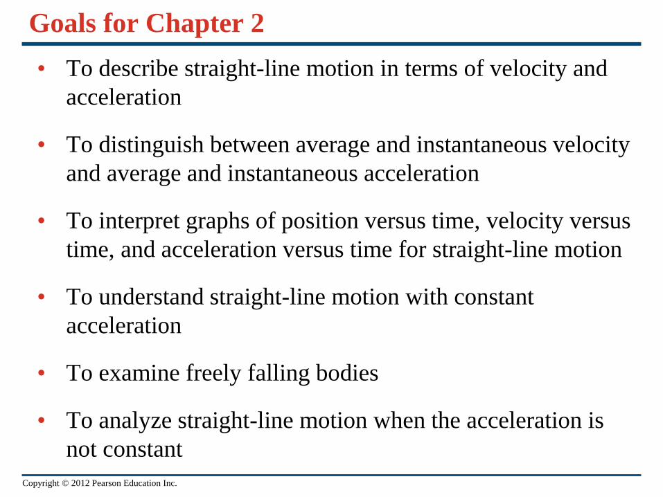
Introduction

• Kinematics is the study of motion.

• Velocity and acceleration are important physical

quantities.

• A bungee jumper speeds up during the first part of his

fall and then slows to a halt.


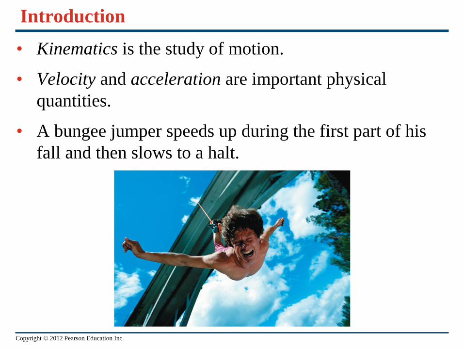
Displacement, time, and average velocity—Figure 2.1

• A particle moving along the x-axis has a coordinate x.

• The change in the particle’s coordinate is x = x2 x1.

• The average x-velocity of the particle is vav-x = x/ t.

• Figure 2.1 illustrates how these quantities are related.


Negative velocity

• The average x-velocity is negative during a time interval if

the particle moves in the negative x-direction for that time

interval. Figure 2.2 illustrates this situation.


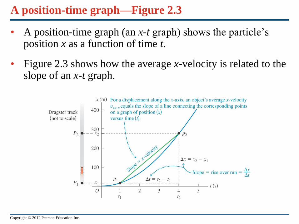
A position-time graph—Figure 2.3

• A position-time graph (an x-t graph) shows the particle’s position x as a function of time t.

• Figure 2.3 shows how the average x-velocity is related to the slope of an x-t graph.


Instantaneous velocity—Figure 2.4

• The instantaneous velocity is the velocity at a

specific instant of time or specific point along the

path and is given by vx = dx/dt.

• The average speed is not the magnitude of the

average velocity!


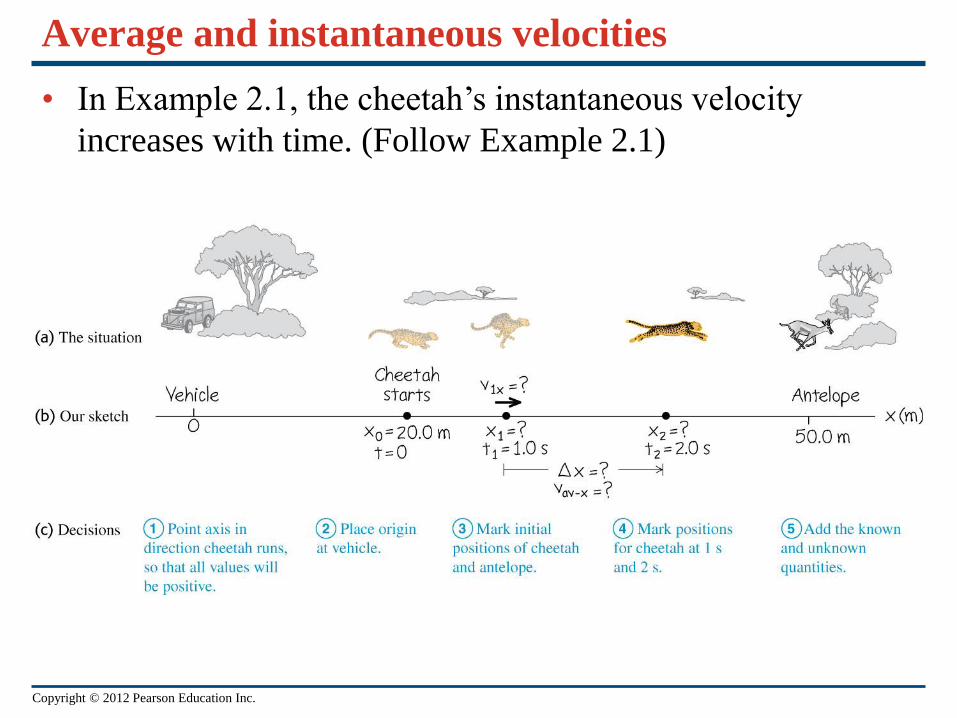
Average and instantaneous velocities

• In Example 2.1, the cheetah’s instantaneous velocity

increases with time. (Follow Example 2.1)


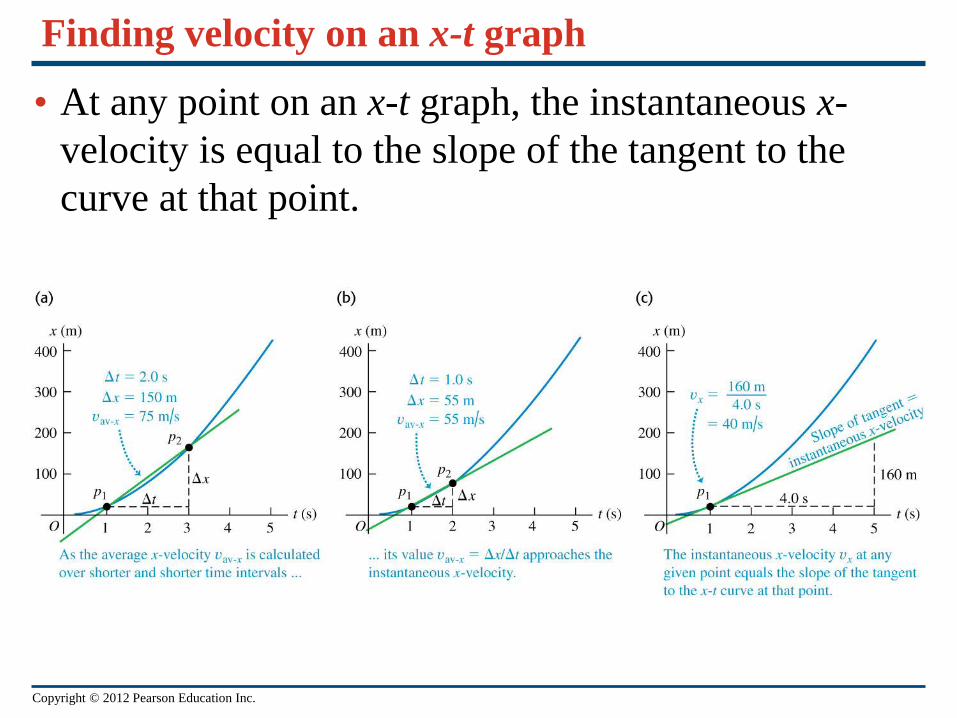
Finding velocity on an x-t graph

• At any point on an x-t graph, the instantaneous x-

velocity is equal to the slope of the tangent to the

curve at that point.


Motion diagrams

• A motion diagram shows the position of a particle at various instants, and arrows represent its velocity at each instant.

• Figure 2.8 shows the x-t graph and the motion diagram for a

moving particle.


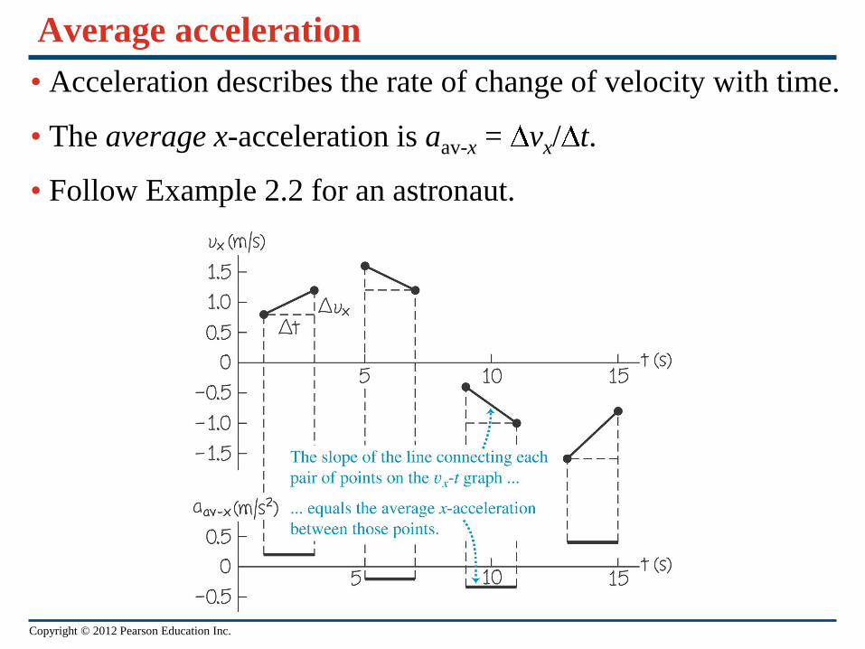
Average acceleration

• Acceleration describes the rate of change of velocity with time.

• The average x-acceleration is aav-x = vx/ t.

• Follow Example 2.2 for an astronaut.


Instantaneous acceleration

• The instantaneous acceleration is ax = dvx/dt.

• Follow Example 2.3, which illustrates an accelerating racing

car.


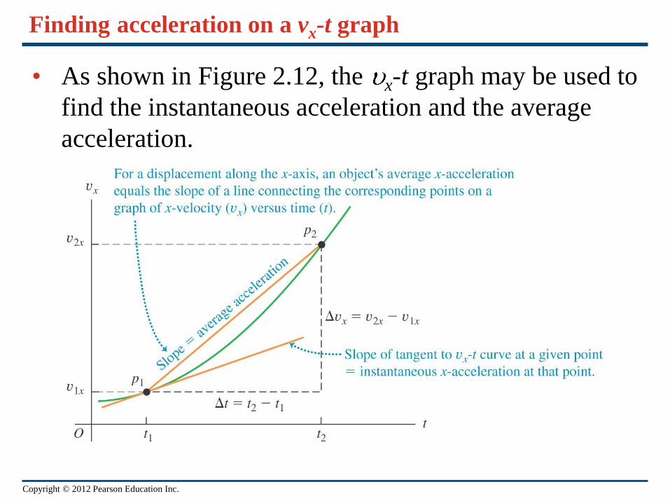
Finding acceleration on a vx-t graph

• As shown in Figure 2.12, the x-t graph may be used to

find the instantaneous acceleration and the average

acceleration.


A vx-t graph and a motion diagram

• Figure 2.13 shows the vx-t graph and the motion diagram

for a particle.


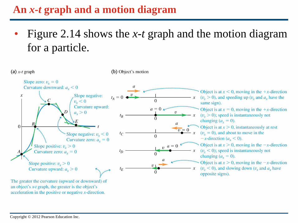
An x-t graph and a motion diagram

• Figure 2.14 shows the x-t graph and the motion diagram

for a particle.


Motion with constant acceleration—Figures 2.15 and 2.17

• For a particle with constant acceleration, the velocity

changes at the same rate throughout the motion.


The equations of motion with constant acceleration

• The four equations shown to

the right apply to any straight-

line motion with constant

acceleration ax.

• Follow the steps in

Problem-Solving Strategy 2.1.

vx v0x

axt

x x0

v0x

t 12

axt2

vx2 v

0x2 2ax x x

0

x x0

v0x

vx

2t


A motorcycle with constant acceleration

• Follow Example 2.4 for an accelerating motorcycle.


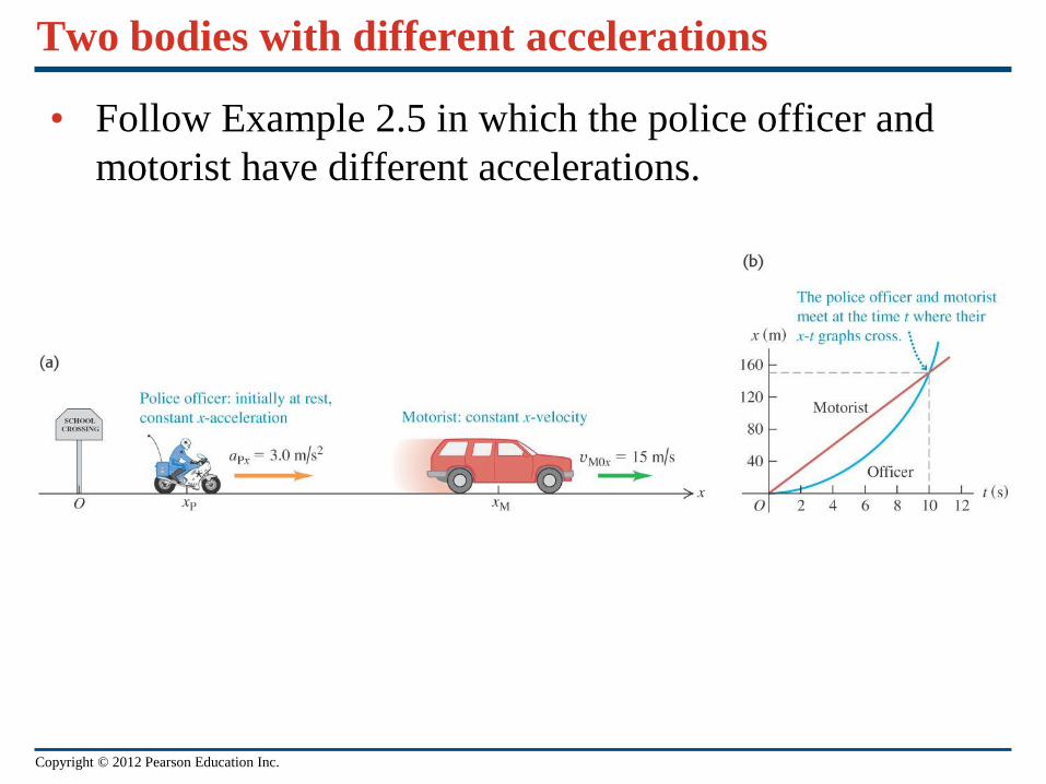
Two bodies with different accelerations

• Follow Example 2.5 in which the police officer and

motorist have different accelerations.


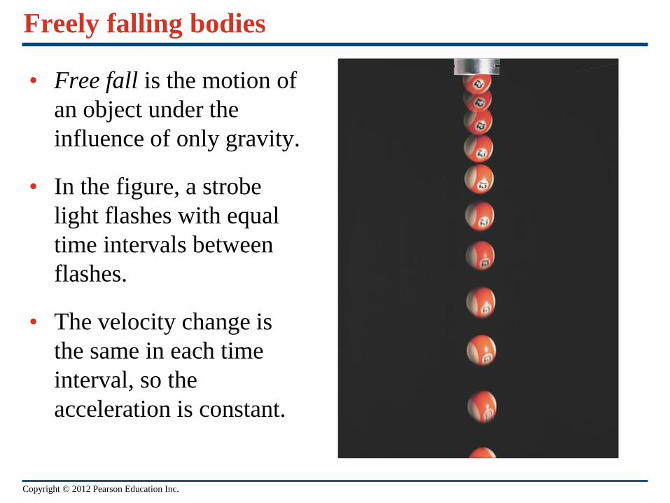
Freely falling bodies

• Free fall is the motion of

an object under the

influence of only gravity.

• In the figure, a strobe

light flashes with equal

time intervals between

flashes.

• The velocity change is

the same in each time

interval, so the

acceleration is constant.


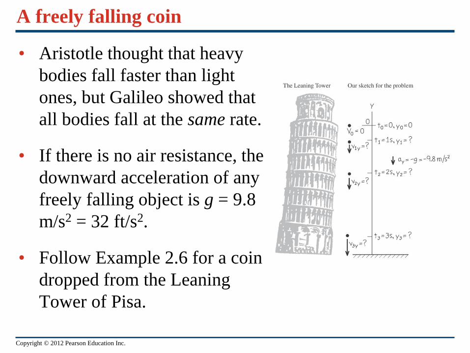
A freely falling coin

• Aristotle thought that heavy

bodies fall faster than light

ones, but Galileo showed that

all bodies fall at the same rate.

• If there is no air resistance, the

downward acceleration of any

freely falling object is g = 9.8

m/s2 = 32 ft/s2.

• Follow Example 2.6 for a coin

dropped from the Leaning

Tower of Pisa.


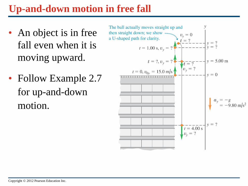
Up-and-down motion in free fall

• An object is in free

fall even when it is

moving upward.

• Follow Example 2.7

for up-and-down

motion.


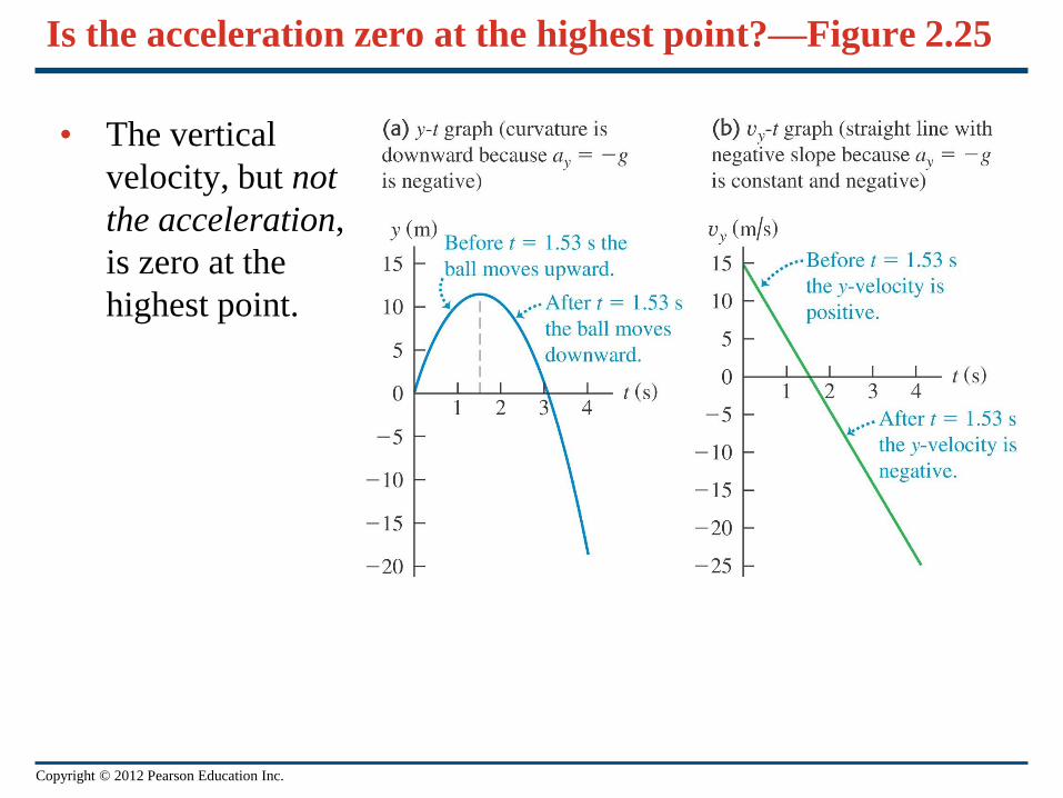
Is the acceleration zero at the highest point?—Figure 2.25

• The vertical

velocity, but not

the acceleration,

is zero at the

highest point.


Two solutions or one?

• We return to the ball in the previous example.

• How many solutions make physical sense?

• Follow Example 2.8.


Velocity and position by integration

• The acceleration of a car is not always constant.

• The motion may be integrated over many small time intervals to

give .00 0

and t t

x ox x xv v a dt x x v dt


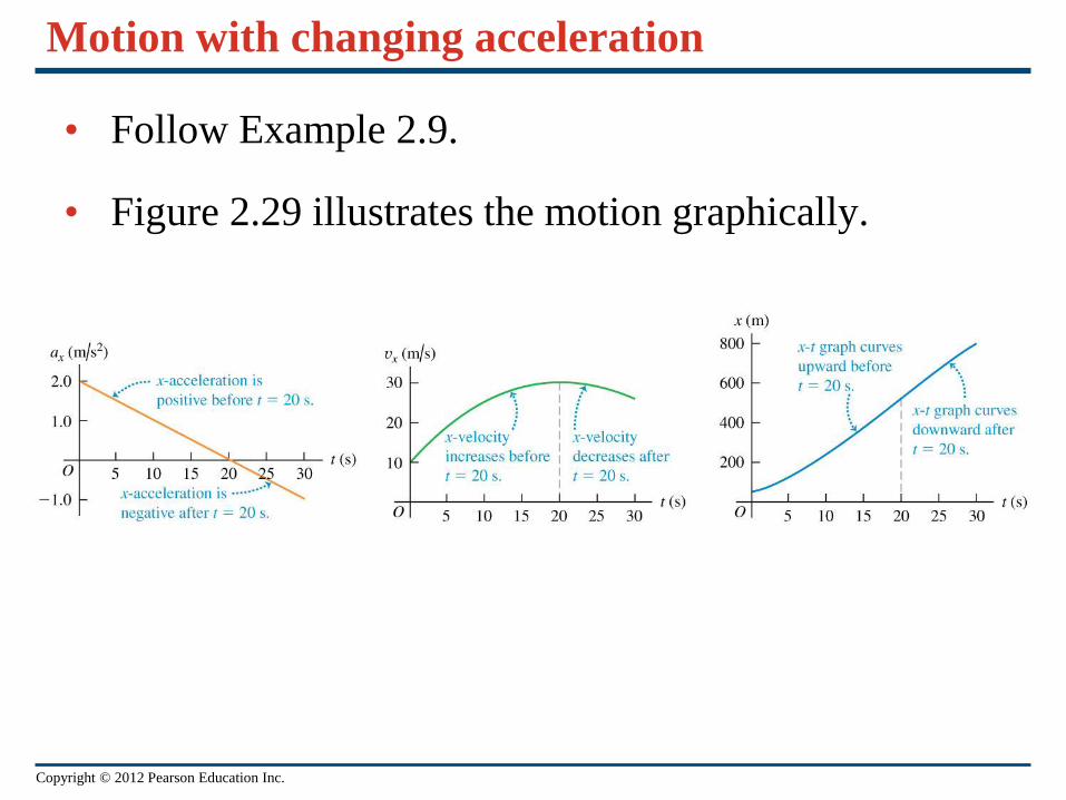
Motion with changing acceleration

• Follow Example 2.9.

• Figure 2.29 illustrates the motion graphically.

Documents

Motion Along a Straight Line - UIC Physicsphysicsweb.phy.uic.edu/141/outline/02_Lecture_Outline.pdfCopyright © 2012 Pearson Education Inc. The equations of motion with constant acceleration