Embed Size (px)
Citation preview

Mortality Dependence and Longevity Bond Pricing:
A Dynamic Factor Copula Mortality Model with the GAS Structure
Hua Chen, Richard D. MacMinn and Tao Sun
April 30, 2014
Hua Chen* Temple University
Email: [email protected]
Richard D. MacMinn Illinois State University
Email: [email protected]
Tao Sun Temple University
Email: [email protected]
*Please address correspondence to: Hua Chen Department of Risk, Insurance, and Health Management Temple University 1801 Liacouras Walk, 625 Alter Hall Philadelphia, PA 19122
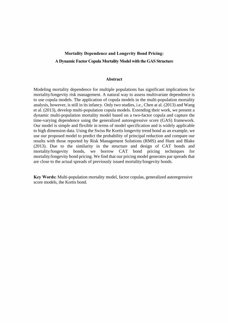
Mortality Dependence and Longevity Bond Pricing:
A Dynamic Factor Copula Mortality Model with the GAS Structure
Abstract
Modeling mortality dependence for multiple populations has significant implications for mortality/longevity risk management. A natural way to assess multivariate dependence is to use copula models. The application of copula models in the multi-population mortality analysis, however, is still in its infancy. Only two studies, i.e., Chen at al. (2013) and Wang et al. (2013), develop multi-population copula models. Extending their work, we present a dynamic multi-population mortality model based on a two-factor copula and capture the time-varying dependence using the generalized autoregressive score (GAS) framework. Our model is simple and flexible in terms of model specification and is widely applicable to high dimension data. Using the Swiss Re Kortis longevity trend bond as an example, we use our proposed model to predict the probability of principal reduction and compare our results with those reported by Risk Management Solutions (RMS) and Hunt and Blake (2013). Due to the similarity in the structure and design of CAT bonds and mortality/longevity bonds, we borrow CAT bond pricing techniques for mortality/longevity bond pricing. We find that our pricing model generates par spreads that are close to the actual spreads of previously issued mortality/longevity bonds.
Key Words: Multi-population mortality model, factor copulas, generalized autoregressive score models, the Kortis bond.

1
1. Introduction
Mortality/longevity risk management is fundamental to the life insurance and
pension industries. Traditionally reinsurance, and more recently, securitization, renders a
means of transferring or hedging mortality/longevity risks. Ever since the issuance of the
first pure mortality bonds in December 2003, Swiss Re has been a major player in this
market and has transferred over $2.2 billion of mortality risk to the capital market. These
mortality bonds are principal-at-risk bonds and their payoffs are usually contingent on
mortality experience of multiple populations (male and female, different age groups and
different countries). Modelling mortality dependency among the indexed populations is
essential; failing to do so would overestimate market prices of risk, thus discouraging risk
transfer by (re)insurers (Lin et al. 2013). In addition to mortality risk in its books of life
business, Swiss Re is also exposed to significant longevity risk in its books of pension
business. These two risks can partially offset each other in a natural hedge, but basis risk
exists when the mortality experiences of the reference populations in these two lines of
business are not exactly the same. In order to hedge the residual longevity risk, Swiss Re
issued the first longevity trend bond via Kortis Capital Ltd. in December 2010; the payoff
is based on the difference in the morality improvements in the US male 55-65 and the UK
male 75-85. Capturing mortality dependence between these two populations is of
significance to Swiss Re for pricing and reserving.
There has been a growing literature on mortality models for multiple populations
in recent years (see, for example, Li and Lee, 2005; Li and Hardy 2011; Dowd et al. 2011;
Jarner and Kryger 2011; Cairns et al., 2011; Yang and Wang, 2013; Zhou et al. 2013a,
2013b). These models are typically structured assuming that the forecasted mortality
2
experiences of two or more related populations are linked together and do not diverge over
the long run. This assumption might be justified by the long-term mortality co-movements.
It seems, however, too strong to model the short-term mortality dependence. From the
pricing perspective, extant research often uses examples such as the previously issued
mortality bonds or the EIB longevity bond which failed to launch. Though the issuance of
the Kortis bond has attracted lots of attention as the first successful longevity trend bond,
Hunt and Blake (2013) are the first to formally analyze the Kortis bond; they use a two-
population mortality model to predict the bond payoff probability but they do not price the
bond issue. We develop a multi-population mortality model based on a two-factor copula
and introduce a time-varying dependence structure using the generalized autoregressive
score (GAS) model. We then use our proposed mortality model to price the Kortis
longevity bond by using existing CAT bond pricing techniques.
Copulas have been studied in both actuarial science and finance to examine
dependencies among risks (Frees and Valdez, 1998; Embrechts et al. 2003). Particularly,
in mortality studies copulas have been applied to model the bivariate survival function of
the two lives of couples (see, e.g., Frees et al. 1996; Carriere 2000; Shemyakin and Youn
2006; Youn and Shemyakin 1999, 2001; Denuit et al. 2001). Surprisingly, the application
of copula models in the multi-population mortality analysis is still in its infancy stage. To
our the best of our knowledge, only two papers, Chen et al. (2013) and Wang et al. (2013),
fall into this category.
A common feature in these two papers is that both build a multi-population
mortality model based on a two-stage procedure. In the first stage, the mortality dynamics
of each population is modeled using a time series analysis. In the second stage, the
3
mortality dependence of the residuals from the first stage is captured using a copula model.
The two-stage procedure permits the separate development of the marginal distributions
and the copula model. Hence, this method allows the use of any existing model for the
univariate analysis with the subsequent focus on the copula model. In spite of the similarity,
their models differ in several ways. First, Chen et al. (2013) choose the best ARMA-
GARCH model for mortality data of each population, whereas Wang et al. (2013) use an
ARIMA (0,1,0) to fit the mortality index estimated from the Lee-Carter model for each
country, ignoring the population-specific condition mean, not to mention the conditional
variance model. Second, Chen et al. (2013) use a one-factor copula model which is widely
applicable to high dimension data and very flexible in terms of model specification, while
Wang et al. (2013) use copulas in the Elliptical or Archimedean family, which usually have
only one or two parameters to characterize the dependence between all variables, and are
thus quite restrictive when the number of variables increases. Third, Chen et al. (2013) find
that the best one-factor model has a common factor with heavy tails and positive skewness,
suggesting that mortality dependence is stronger during mortality deteriorations than
during mortality improvements. This conforms to the conjecture that mortality jumps due,
for example, to rare pandemic events are more likely to occur simultaneously. In contrast,
Wang et al. (2013) note that mortality dependence may be asymmetric, they use four
copulas in their study (Gaussian, Student-t copula, Gumbel and Clayton copula), among
which Student-t copula provides the best fit. Hence they fail to capture the asymmetric tail
dependence of mortality rates across countries. Finally, Wang et al. (2013) adopt the
dynamic conditional correlation (DCC) approach in the copula model to allow correlations
to change over time, but Chen et al. (2013) only consider a static approach.

4
In this paper, we adopt the factor copula to model mortality dependence because of
its simplicity and flexibility. The factor copula is based on a simple linear, additive factor
structure for the copula and is particularly attractive for high dimension applications. Next,
the factor copula permits more flexibility for the number of variables and available data.
We extend the one-factor copula model used in Chen et al. (2013) to a two-factor copula
model, with one common factor representing the market force which drives mortality
dynamics for all countries and one country-specific factor capturing mortality dependence
across different age groups in each country.
We also incorporate the time-varying structure into the factor model by using the
Generalized Autoregressive Score (GAS) framework. The GAS model was developed by
Creal et al. (2013) who argue that the score function is an effective choice for introducing
a driving mechanism for time-varying parameters. Oh and Patton (2013) use the lagged
score of the copula model as the forcing variable to drive the factor loadings of conditional
factor copulas over time and use this dynamic factor copula model to study Credit Default
Swap (CDS) spreads on 100 US firms. As GAS models are observation-driven time-
varying parameter models, their copula models do not require the additional integration
over the path of the latent variables in order to calculate the likelihood. We adopt a similar
approach in this paper to capture the time-varying mortality dependence for multiple
populations.
Mortality/longevity securities involve significant valuation problems. Financial
pricing approaches emphasize the creation of replicating portfolios (Black and Scholes,
1973; Merton, 1973) or the existence of a unique risk-neutral measure (Cox and Ross, 1976;
Harrison and Kreps, 1979; Harrison and Pliska, 1981) in a complete market. In an

5
incomplete market, the non-arbitrage condition ensures the existence of at least one risk-
neutral measure. We, however, do not have clues regarding the appropriate choice of the
risk-neutral measure with sparse market price data. This difficulty drives us to choose
alternative insurance pricing approaches in CAT bond markets, which determines CAT
bond premiums based on expected loss plus a risk loading. The risk loading can be
proportional to expected loss itself, or proportional to the variance or standard deviation of
the loss, or is determined by a risk cubic model based on two other risk factors, i.e.,
probability of first loss (PFL) and conditional expected loss (CEL), to capture the trade-off
between the frequency and severity of the loss (Lane and Movchan, 1999; Lane, 2000).
Mortality/longevity bonds are similar to CAT bonds in structure and design, so CAT bond
pricing methodologies can be equally applied to mortality/longevity bonds. Lane (2000)
uses the risk cubic model to price the Vita I and II mortality bonds. Chen and Cummins
(2010) find that the risk cubic model can exactly replicate the risk premium of the Vita I
mortality bond. They therefore employ the cubic model to explicitly derive risk premia for
a proposed longevity bond. We follow the same approach but include some bond-specific
characteristics, such as size, maturity, trigger, peril, and region, into our pricing model to
explain CAT bond premiums, in addition to risk measures of the loss distribution (i.e., EL,
PFL and CEL).
Our paper contributes to the existing literature in several ways. First, we are among
the first to develop a copula-based mortality model to capture morality correlations among
multiple populations. Copulas are powerful tools to model the dependence for tail events
or extreme risks, therefore our model has significant applications to mortality risk pricing
and hedging for correlated risks. Second, we extend the one-factor copula model to two-

6
factor copula model, so our model can capture not only the mortality dependence across
countries but also mortality dependence across age groups in each country. Third, we
incorporate the time-varying dependence structure in our factor copula model, leading to a
flexible yet parsimonious dynamic model for high dimension conditional distributions.
Finally, we apply the CAT bond pricing model to mortality/longevity bonds. We find our
model generates prices that are close to those observed in these transactions.
The remaining of this paper is organized as follows. In Section 2, we introduce the
structure design of the Kortis longevity bond. In Section 3, we propose our multi-
population mortality model with dynamic dependence based on a factor copula approach
and the generalized autoregressive score model. In Section 4, we investigate mortality data
for US male 55-65 and UK male 75-85 and estimate the parameters in our mortality model.
In Section 5, we discuss the CAT bond pricing methodologies and apply it to price the
Kortis longevity bond. Concluding remarks are given in Section 6.
2. The Kortis Longevity Bond
Swiss Re has a strong track record of developing the capital markets for insurance
perils, initially with natural catastrophe bonds and more recently by periodically
securitizing its life risks. To hedge that risk, it has sold about $2.2 billion in mortality bonds
to date. Such bonds earn a healthy yield, so long as there’s no big rise in mortality. If there
is, then the bondholders lose some or all of their principal, and it’s used instead to make
those unexpected life-insurance payouts. We summarize some characteristics of
mortality/longevity bonds issued to date and report them in Table 1.

7
Table 1: Mortality/Longvity Bonds Issued to Date
Vita I Vita II Tartan Osiris Vita III Nathan
Sponsor Swiss Re Swiss Re Scottish Re AXA Swiss Re Munich Re
Arranger Swiss Re Swiss Re Goldman Sachs Swiss Re Swiss Re Munich Re
Modelling Firm Milliman Milliman Milliman Milliman Milliman Milliman
SPV domicile Cayman Islands Cayman Islands Cayman Islands Ireland Cayman Islands Cayman Islands
Size $400M $362M $155M €345M $705M $100M
No. of Tranches 1 3 2 3 2 1
Issue date December 2003 April 2005 May 2006 November 2006 January 2007 February 2008
Maturity 4 years 5 years 3 years 4 years 4 & 5 years 5 years
Index US, UK, France, Italy, Switzerland
US, UK, Germany, Japan, Canada
US France, Japan, US US, UK, Germany, Japan, Canada
US, UK, Canada, Germany
Vita IV Kortis Vita IV Vita V Atlas IX
Sponsor Swiss Re Swiss Re Swiss Re Swiss Re SCOR Re
Arranger Swiss Re Swiss Re Swiss Re Swiss Re Aon, BNP Paribas, Natixis
Modelling Firm RMS RMS RMS RMS RMS
SPV domicile Cayman Islands Cayman Islands Cayman Islands Cayman Islands Ireland
Size $300M $50M $180M $275M $180M
No. of Tranches 4 1 2 2 2
Issue date
I: November 2009 II: May 2010 III: October 2010 IV: October 2010
December 2010 July 2011 July 2012 September 2013
Maturity 4 & 5 years 6 years 5 years 5 years 5 years
Index
I :US, UK II: US/UK III: US/Japan IV: Germany/Canada
US, UK IV: Canada/German V:Canada/Germany/UK/US
D-1: Australia, Canada E-1: Australia, Canada, US
US

8
On the other hand, as ageing baby boomers put pension fund balances under
increasing pressure, global exposure to longevity risk involves about $20.7 trillion of
pension assets (Swiss Re, 2012). Heavyweight reinsurers are renewing their efforts to
provide capacity for longevity risk. As an example, Swiss Re announced in 2009 that it
would insure around £1 billion of pensioner liabilities for the Royal County of Berkshire
Pension Fund. Insuring longevity risk, then, is a great deal for Swiss Re: not only should it
be profitable, if it’s priced correctly, but it also helps to naturally hedge the company’s
mortality risk.
Such natural hedge is perfect - basis risk can arise from two sources. First, trends
in mortality improvement can be different in the US and UK, owing to the different
lifestyles and medical systems operating on either side of the Atlantic. Second, annuity
policyholders or pensioners are typically older than life assurance policyholders and rates
of longevity improvement differ across ages. If the reference population in the pension pool
experiences a much greater mortality improvement than those with the life pool then the
natural hedge is not sufficient protection.
In order to transfer the residual longevity risk between its books of pension and life
insurance business, Swiss Re sold $50 million of the first “longevity trend” bonds to capital
market investors via a Cayman Island domiciled, off-balance-sheet vehicle called Kortis
Capital Ltd., in December 2010. The bond pays quarterly coupons at a spread of 5.0%
above the three-month LIBOR and matures in January 2017 (extendable until July 2019).
The principal repayment is indexed on a Longevity Divergence Index Value (LDIV),
defined as the divergence in the mortality improvements experienced between male lives
aged 75-85 in England & Wales, which can be seen as representing Swiss Re’s pension

9
exposures, and male lives aged 55-65 in the US, which can be seen as representing Swiss
Re’s life insurance exposure (Swiss Re, 2012).
The LDIV is constructed in several steps. First, the mortality improvement in each
population for men at different ages is averaged over n years, i.e.,
1/
,
,
, 1
njx tj
x jx t n
mm t n t
m
where ,jx tm is the crude mortality rate observed at age x in year t for population j and n is
the averaging period of the bond. An averaging period of eight years is used to calculate
the observed improvement, so that the Kortis bond is indexed to changes in mortality rates
over the period 1 January 2009 to 31 December 2016.
Second, the mortality improvement is then averaged across age groups (ages 1x to
2x ) for each year and country, i.e.,
2
1
1 22 1
1, 8,
1
xj j
t xx x
m x x m t tx x
.
To take into account the fact that pensioners are typically older than life insurance
policyholders, EW 75,85tm is calculated using ages between ages 75 and 85 for England
& Wales, while US 55,65tm is calculated using ages between 55 and 65 in the US.
Finally, the longevity divergence index value (LDIV) is calculated for year t as
EW USLDIV 75,85 55,65t t tm m .
The “principal reduction factor” (PRF) is indexed on the LDIV and structured as a
call option spread, similar to the Vita programs, i.e.,
2016 2016LDIV 3.4% LDIV 3.9%PRF
3.9% 3.4%
,
10
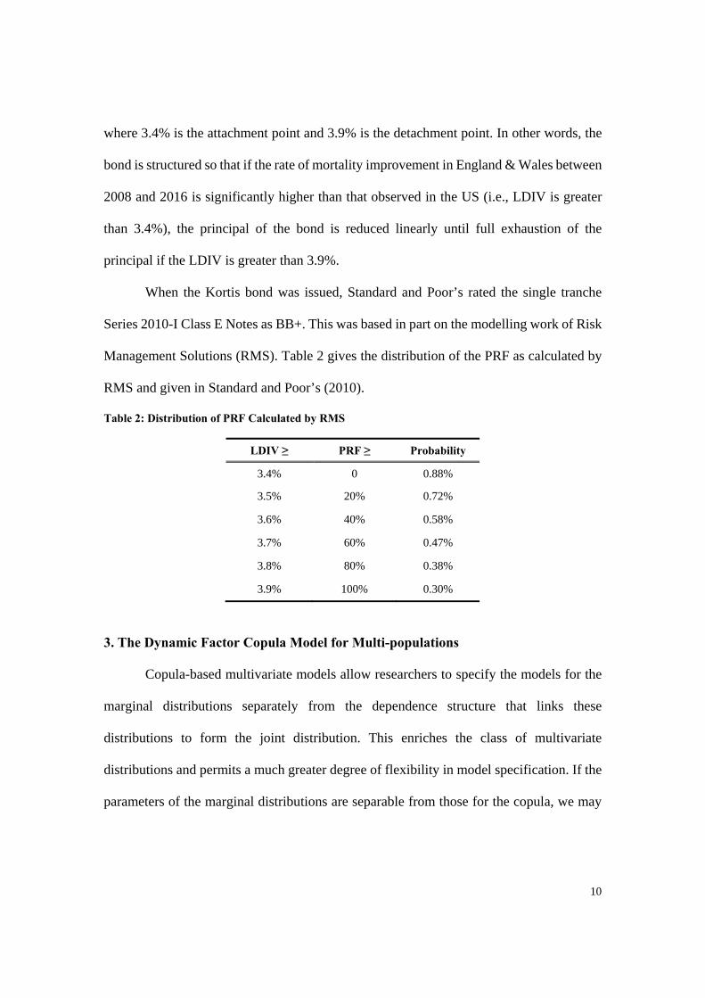
where 3.4% is the attachment point and 3.9% is the detachment point. In other words, the
bond is structured so that if the rate of mortality improvement in England & Wales between
2008 and 2016 is significantly higher than that observed in the US (i.e., LDIV is greater
than 3.4%), the principal of the bond is reduced linearly until full exhaustion of the
principal if the LDIV is greater than 3.9%.
When the Kortis bond was issued, Standard and Poor’s rated the single tranche
Series 2010-I Class E Notes as BB+. This was based in part on the modelling work of Risk
Management Solutions (RMS). Table 2 gives the distribution of the PRF as calculated by
RMS and given in Standard and Poor’s (2010).
Table 2: Distribution of PRF Calculated by RMS
LDIV ≥ PRF ≥ Probability
3.4% 0 0.88%
3.5% 20% 0.72%
3.6% 40% 0.58%
3.7% 60% 0.47%
3.8% 80% 0.38%
3.9% 100% 0.30%
3. The Dynamic Factor Copula Model for Multi-populations
Copula-based multivariate models allow researchers to specify the models for the
marginal distributions separately from the dependence structure that links these
distributions to form the joint distribution. This enriches the class of multivariate
distributions and permits a much greater degree of flexibility in model specification. If the
parameters of the marginal distributions are separable from those for the copula, we may

11
estimate those parameters separately in two stages, which greatly simplifies the estimation
procedure and facilitates the study of high-dimension multivariate problems. 1
2.1. The First Stage: The Conditional Marginal Distribution
Suppose we need to model the dependence structure of time series data, ity ,
1, 2,..., 1, 2,...,i N t T , . We first model the conditional marginal distribution of ity . We
allow each time series to have a time-varying conditional mean and conditional variance,
each governed by parametric models,
1 1it i t i t ity Z Z for 1, 2,...,i N and 1 1t tZ F , (1)
where 1i tZ and 1i tZ denote the functional forms for the conditional mean and
conditional volatility, 1tF is the sigma-field containing information generated by
1 2{ , , }t ty y .
The estimate of standardized residuals can be specified as
1
1
ˆ;ˆ
ˆ;it i t
iti t
y Z
Z
, (2)
where 1 ˆ;i tZ and 1 ˆ;i tZ are the estimated conditional mean and conditional
volatility with the vector of estimated parameters .
We then estimate the distribution of the standardized residuals using the empirical
distribution function (EDF), denoted as iF for variable i,
1
1ˆ ˆ1
T
i itt
FT
1 . (3)
1 Clearly, two- or multiple-stage estimation is asymptotically less efficient than one-stage estimation. However, simulation studies in Joe (2005) and Patton (2006) indicate that this loss is not great in many cases.
12
where it 1 is an indicator function which is equal to 1 when it and 0 otherwise.
The use of the EDF allows us to non-parametrically capture skewness and excess
kurtosis in the residuals, if present, and allows these characteristics to differ across the
mortality time series of each population.
2.2. The Second Stage: A Factor Copula Approach
In the mortality/longevity securitization, we intend to capture the joint distribution
of tail risks, which relies on the dependence structure of the innovation process. A
straightforward approach is to use a copula model to describe the joint distribution of
innovations. With the EDF, the copula model for the standardized residuals can be
structured as
11 , , ~ , , ;
N
T
t t Nt iid F C F F . (4)
The copula is parameterized by a vector of parameters, , which can be estimated
using the simulation-based estimation approach proposed by Oh and Patton (2012). Their
method is close to Simulated Method of Moments (SMM), but is not exactly the same as
SMM, because the “moments” that are used in estimation are functions of rank statistics.
The SMM copula estimator is based on simulation from some joint distribution of a vector
of latent variables X , XF , with implied copula C . Briefly speaking, we estimate
the vector of parameters, , by minimizing the sum squared errors between moment
conditions (i.e., dependence measures) computed using simulations from XF and those
computed from standardized residuals 1
ˆ T
t t
. The details of the simulated-based method
of moments are given in Appendix A.
In this study, we consider a two-factor model proposed by Oh and Patton (2012),

13
which is generated by the following structure
1
00
0
1
~ , US or UK;
~ , 1,..., ; ,
, , ~ , ,
c
N
ci i i c i
c Z c
i i j
N X X X
X Z Z
Z iid F c Z Z c
iid F i N Z i j
X X X F C F F
, (5)
where iX are latent variables, 0Z is the common, market-wide, factor that affects both US
and UK mortality rates, cZ is the country factor that affect US or UK mortality rates only,
and i are idiosyncratic factors. It is noteworthy that we impose the same dependence
structure, or the copula model, for the latent variables X and the original variables i but
their marginal distributions might be different.
This class of factor copula models has a simple form but a very flexible dependence
structure. For example, by allowing for a fat-tailed common factor the model captures the
possibility of correlated crashes in different markets or correlated mortality jumps in
different countries. By assuming a skewed distribution on the common factor the model
allows for an asymmetric tail dependence structure, which is consistent with the fact that
the stock returns are more correlated in crashes than in booms or mortality dependence is
stronger during mortality deteriorations than during mortality improvements. If we impose
the same loading on the common factor we have an equidependence structure, whereas
different loadings on the common factor enable us to model heterogeneous pairs of
variables at the cost of a more difficult estimation problem. We can also simplify the
problem by assuming sub-sets of variables (for example, mortality rates for countries in
the same continent or those for different age groups in the same country) have the same
loading on the common factor. Furthermore, the one-factor model can be extended to multi-
14
factor models to capture heterogeneous pair-wise dependence within the overall
multivariate copula.
2.3. Dynamic Dependence with GAS
The static factor copula model specified in equation (4) and (5) can be extended to
a dynamic factor copula model that can capture time-varying dependence in high
dimensions. For instance, we can allow the factor loadings, ,i i , to be time-varying, or let
the “shape” parameters, ,of the factors 0Z , cZ to be time dependent. As a balance between
the model flexibility and feasibility, we assume that the factor loading parameters are time-
varying and the “shape” parameters of the factors 0Z , cZ to be fixed through time, which
are similar to Oh and Patton (2013).
1
0, 0 ,
1 1 1
0 01, , , ,
, 1,...,
, , ~ ( ( )), , ( ( )) , 1,...,
,... , ,..., '
t t Nt
cit i t i t c i
t t Nt X X t X t
c ct t N t i t i t
X Z Z i N
X X X F C F F t T
, (6)
An important feature of any dynamic model is the specification for how the
parameters evolve through time. We adopt the generalized autoregressive score (GAS)
model of Creal et al. (2013) to model the dynamics of factor loading parameters. These
authors propose using the lagged score of the density model (copula model, in our
application) as the forcing variable. Specifically, for a copula with time-varying parameter
t , governed by fixed parameter , we have:
Let 1t t tU F C
Then 1 1t t tw B As , (7)
where 1 1 1t t ts S
15
1 11
1
log ;t tt
t
c u
and tS is a scaling matrix (e.g., the inverse Hessian or its square root). This specification
has several advantages: firstly, compared with modeling the time-vary parameters as a
latent time series, such as stochastic volatility models (see, e.g., Shephard 2005) and related
stochastic copula models (Hafner and Manner 2011; Manner and Segers 2011), modeling
the varying parameter as some functions of observable avoids the need to “integrate out”
the innovation terms driving the latent time series processes, which is very important for
the tractability of the model in high dimensions. Secondly, the GAS model exploits the
complete density structure to update the time-varying parameter based on density score
rather than means and higher moment only. Thirdly, the recursion using the density score
as the forcing variable can be justified as the steepest ascent direction for improving the
model’s fit, in terms of the likelihood, given the current value of the model parameter t .
In the general GAS framework in equation (7), the 2N time-varying factor
loadings in equation (6) would require the estimation of 22(2 )N N parameters governing
their evolution, which represents an infeasibly large number for even moderate values of
N . To keep the model parsimonious, we impose that the coefficient matrices (B and A)
are diagonal with a common parameter on the diagonal, as in the DCC model of Engle
(2002). To avoid the estimation of N N scaling matrix we set tS I . This simplifies the
evolution model for time-varying parameters to be (in logs):
, 1, , 1log log , {0, }i t
j ji t i i ts j c
(8)
16
where0
log ( ; , , , ) /c it
jit t t z zs c u λ an 0 0
1, , 1, ,,... , ,..., 'c ct t N t t N t . Lastly, we adopt
the “variance target” method proposed in Oh and Patton (2013) to further simplify the
estimation of i in equation (8). Using the result from Creal, et al. (2013) that 1 0t itE s ,
we have log / (1 )jit iE equation (8) can be rewrite as
, 1 , 1log log (1 ) logit it i t
j j ji tE s
(9)
where log tE can be pre-estimated using sample rank correlation (see Proposition 1 in
Oh and Patton, 2013). After the above reductions, we only need to estimate the following
parameters in the dynamic copula model implied by equations (6) and (9): two parameters
for the GAS dynamics (i.e. , ) and the shape parameters for the common, country and
idiosyncratic factors.
4.Model Estimation
4.1. Data
We collect mortality data for US and UK (England & Wales) from Human
Mortality Database over the period 1933-2010.2 This sample period is determined by US
mortality data, which is available only after year 1933. To be consistent with the Swiss Re
Kortis bond, we choose UK males with ages 75 to 85 and US males with ages 55 to 65.
4.2. Conditional Marginal Distribution
Denote ,jx tm the crude mortality rate at age x in year t for country j. Figure 1 plots
the crude mortality rates for UK male aged 75-85 and US male aged 55-65 from 1933 to
2010. We observe a clear trend of mortality improvements for all age groups, and a very
2 Data source: Human Mortality Database, available at www.mortality.org

17
strong intra-group dependence of mortality dynamics in each country. We also find the
evidence of the cohort effect. For example, a small hump in the mortality rate for UK male
aged 75 in 1994 was passed on to subsequent years when this age group grew older. The
US age groups exhibit even stronger cohort effect than the UK age groups. Clearly these
mortality rates are not stationary. So we compute the first difference of the logged mortality
rates, denoted by , , , 1ln lnj j jx t x t x ty m m , to obtain the mortality rate changes over time, as
can be seen in Figure 2.3
Figure 1: Mortality Rates for US male 55-65 and UK male 75-85
3 A positive
( )ity indicates mortality deterioration and a negative
( )ity suggests morality improvement.
1940 1950 1960 1970 1980 1990 2000 20100
0.05
0.1
0.15
0.2
0.25
0.3
Year
Mor
talit
y R
ate
UK Mortality Rate(Age75-85,Year1933-2010)
7576777879808182838485
1940 1950 1960 1970 1980 1990 2000 20100.005
0.01
0.015
0.02
0.025
0.03
0.035
0.04
Year
Mor
talit
y R
ate
US Mortality Rate(Age55-65,Year1933-2010)
5556575859606162636465
18
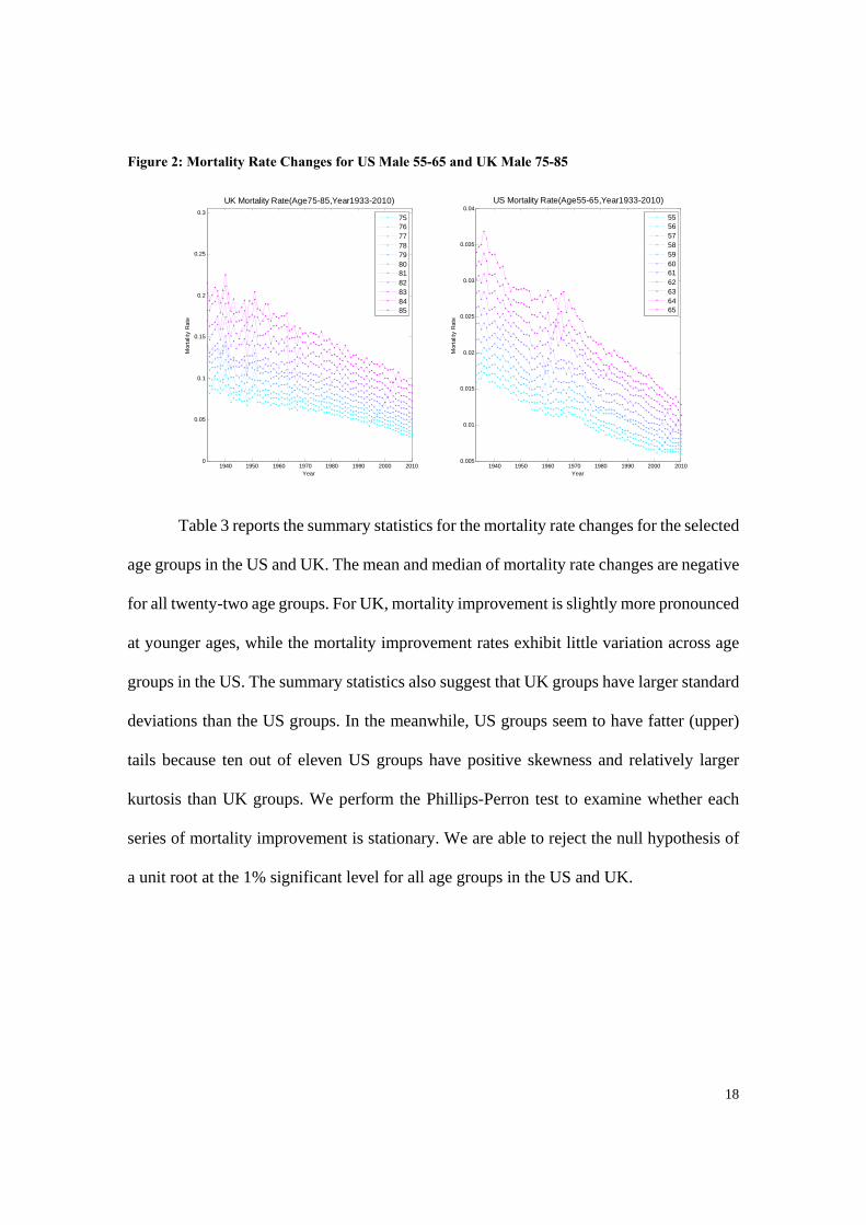
Figure 2: Mortality Rate Changes for US Male 55-65 and UK Male 75-85
Table 3 reports the summary statistics for the mortality rate changes for the selected
age groups in the US and UK. The mean and median of mortality rate changes are negative
for all twenty-two age groups. For UK, mortality improvement is slightly more pronounced
at younger ages, while the mortality improvement rates exhibit little variation across age
groups in the US. The summary statistics also suggest that UK groups have larger standard
deviations than the US groups. In the meanwhile, US groups seem to have fatter (upper)
tails because ten out of eleven US groups have positive skewness and relatively larger
kurtosis than UK groups. We perform the Phillips-Perron test to examine whether each
series of mortality improvement is stationary. We are able to reject the null hypothesis of
a unit root at the 1% significant level for all age groups in the US and UK.
1940 1950 1960 1970 1980 1990 2000 20100
0.05
0.1
0.15
0.2
0.25
0.3
Year
Mor
talit
y R
ate
UK Mortality Rate(Age75-85,Year1933-2010)
7576777879808182838485
1940 1950 1960 1970 1980 1990 2000 20100.005
0.01
0.015
0.02
0.025
0.03
0.035
0.04
Year
Mor
talit
y R
ate
US Mortality Rate(Age55-65,Year1933-2010)
5556575859606162636465

19
Table 3: Summary Statistics for mortality improvements
Age No. of Obs Mean Std. Dev Median Min Max Skewness Kurtosis
UK75 77 -0.0141 0.0499 -0.0160 -0.1398 0.1538 0.3582 4.5500
UK76 77 -0.0143 0.0543 -0.0179 -0.1541 0.1265 0.0068 3.6428
UK77 77 -0.0137 0.0523 -0.0167 -0.1457 0.1352 0.0631 3.8443
UK78 77 -0.0137 0.0508 -0.0102 -0.1516 0.1400 0.1781 3.9124
UK79 77 -0.0133 0.0550 -0.0159 -0.1524 0.1396 0.2660 3.6663
UK80 77 -0.0129 0.0515 -0.0163 -0.1501 0.1262 -0.2525 3.5902
UK81 77 -0.0115 0.0512 -0.0111 -0.1415 0.1222 -0.1110 3.0261
UK82 77 -0.0125 0.0553 -0.0159 -0.1527 0.0958 -0.3692 3.1232
UK83 77 -0.0120 0.0590 -0.0152 -0.1535 0.1108 -0.3055 3.0358
UK84 77 -0.0117 0.0517 -0.0053 -0.1396 0.1029 -0.2580 3.0568
UK85 77 -0.0111 0.0572 -0.0078 -0.1501 0.1476 -0.1128 2.9797
US55 77 -0.0125 0.0301 -0.0144 -0.0702 0.0954 0.4832 4.0686
US56 77 -0.0122 0.0279 -0.0116 -0.0862 0.0858 0.1399 4.3162
US57 77 -0.0123 0.0278 -0.0150 -0.0737 0.0782 0.2449 3.6865
US58 77 -0.0124 0.0315 -0.0164 -0.0988 0.0861 0.2061 4.2160
US59 77 -0.0128 0.0313 -0.0125 -0.1383 0.0773 -0.4744 5.6521
US60 77 -0.0133 0.0319 -0.0132 -0.0912 0.0950 0.4094 4.2988
US61 77 -0.0136 0.0322 -0.0152 -0.0936 0.1053 0.6199 5.3628
US62 77 -0.0135 0.0337 -0.0148 -0.1214 0.1067 0.4639 5.4813
US63 77 -0.0127 0.0302 -0.0170 -0.0911 0.1173 1.1282 6.8815
US64 77 -0.0135 0.0260 -0.0126 -0.0862 0.0704 0.1689 4.0406
US65 77 -0.0126 0.0288 -0.0134 -0.1047 0.0761 0.2808 4.5029
Based on the Box-Jenkins (1976) approach, we fit the mortality rate changes with
a conditional mean model ARMA (r, m)
1 1
+r m
t i t i j t j ti j
y c y
, (6)
20
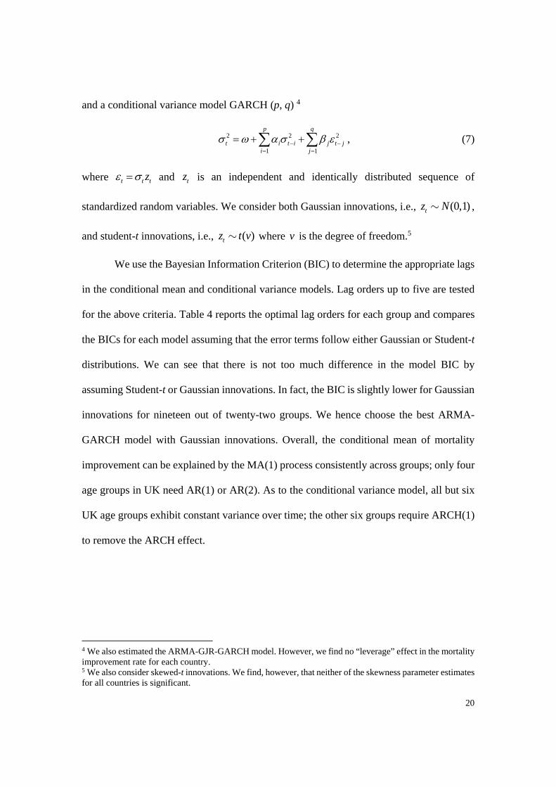
and a conditional variance model GARCH (p, q) 4
2 2 2
1 1
p q
t i t i j t ji j
, (7)
where t t tz and tz is an independent and identically distributed sequence of
standardized random variables. We consider both Gaussian innovations, i.e., (0,1)tz N ,
and student-t innovations, i.e., ( )tz t v where v is the degree of freedom.5
We use the Bayesian Information Criterion (BIC) to determine the appropriate lags
in the conditional mean and conditional variance models. Lag orders up to five are tested
for the above criteria. Table 4 reports the optimal lag orders for each group and compares
the BICs for each model assuming that the error terms follow either Gaussian or Student-t
distributions. We can see that there is not too much difference in the model BIC by
assuming Student-t or Gaussian innovations. In fact, the BIC is slightly lower for Gaussian
innovations for nineteen out of twenty-two groups. We hence choose the best ARMA-
GARCH model with Gaussian innovations. Overall, the conditional mean of mortality
improvement can be explained by the MA(1) process consistently across groups; only four
age groups in UK need AR(1) or AR(2). As to the conditional variance model, all but six
UK age groups exhibit constant variance over time; the other six groups require ARCH(1)
to remove the ARCH effect.
4 We also estimated the ARMA-GJR-GARCH model. However, we find no “leverage” effect in the mortality improvement rate for each country. 5 We also consider skewed-t innovations. We find, however, that neither of the skewness parameter estimates for all countries is significant.

21
Table 4: Conditional Mean and Variance Model selection
Student t Innovation Gaussian Innovation
Group AR MA ARCH GARCH BIC AR MA ARCH GARCH BIC
UK75 0 1 1 0 -255.42 0 1 1 0 -259.74
UK76 1 3 0 0 -228.86 0 1 0 0 -230.26
UK77 0 1 0 0 -237.85 0 1 0 0 -238.47
UK78 0 1 0 0 -241.38 0 1 0 0 -242.02
UK79 0 1 0 0 -227.12 0 1 0 0 -230.22
UK80 1 2 0 0 -250.37 0 1 0 0 -250.88
UK81 0 1 0 0 -247.15 0 1 0 0 -250.12
UK82 0 1 0 0 -236.01 0 1 0 0 -238.05
UK83 0 1 1 0 -241.91 0 1 1 0 -246.37
UK84 0 1 0 0 -250.76 0 1 0 0 -249.53
UK85 0 1 0 0 -240.71 0 1 0 0 -243.81
US55 0 1 0 0 -315.22 0 1 0 0 -318.37
US56 1 0 0 0 -325.69 1 0 0 0 -328.23
US57 1 0 0 0 -328.59 1 0 0 0 -329.99
US58 0 1 0 0 -315.25 1 0 0 0 -317.01
US59 4 0 1 0 -310.82 2 0 1 0 -315.12
US60 0 1 0 0 -311.98 0 1 0 0 -313.81
US61 0 1 1 0 -310.11 0 1 1 0 -311.15
US62 2 0 0 0 -310.03 0 1 0 0 -305.54
US63 1 2 1 0 -314.15 0 1 1 0 -313.56
US64 0 1 0 0 -336.46 0 1 0 0 -337.21
US65 2 2 1 0 -321.72 0 1 1 0 -325.98
After the ARMA-GARCH fitting, we perform the Ljung-Box-Pierce Q tests on the
standardized residuals (the innovations divided by the conditional standard deviations) and
the squared standardized residuals. The results are reported in Table 5. Almost all test
statistics are insignificant up to lag 10, which indicates that our selected model for each
group sufficiently accounts for serial correlation and conditional heteroskedasticity.

22
Table 5: Ljung-Box-Pierce Q tests on standardized residuals and squared standardized residuals
Group
Q Test on the Standardized Innovations
Q Test on the Squared Standardized Innovations
Lag1 Lag5 Lag10 Lag1 Lag5 Lag10
UK75 0.4462
(0.5042) 5.6052
(0.3466) 23.8771 (0.0079)
0.6339 (0.4259)
3.4443 (0.6318)
8.3656 (0.5932)
UK76 0.6511
(0.4197) 8.2136
(0.1448) 21.2038 (0.0197)
1.6446 (0.1997)
19.1480 (0.0018)
33.5358 (0.0002)
UK77 0.1164
(0.7329) 6.7092
(0.2432) 12.0049 (0.2847)
0.8462 (0.3576)
9.2531 (0.0994)
14.5891 (0.1478)
UK78 0.0464
(0.8295) 2.2922
(0.8074) 10.2409 (0.4196)
0.0791 (0.7785)
6.7596 (0.2391)
9.9134 (0.4481)
UK79 0.1109
(0.7391) 13.8121 (0.0168)
19.5255 (0.0341)
3.6274 (0.0568)
15.4603 (0.0086)
21.1747 (0.0199)
UK80 0.0274
(0.8684) 6.0453
(0.3018) 12.8458 (0.2324)
2.3037 (0.1291)
13.8355 (0.0167)
31.4549 (0.0005)
UK81 0.0086
(0.9260) 2.8072
(0.7297) 12.9824 (0.2247)
1.2865 (0.2567)
10.1163 (0.0720)
19.4482 (0.0349)
UK82 0.3295
(0.5660) 5.2009
(0.3919) 11.1723 (0.3443)
0.5974 (0.4396)
5.6165 (0.3453)
13.9813 (0.1738)
UK83 1.6642
(0.1970) 2.6454
(0.7545) 20.2634 (0.0269)
0.4149 (0.5195)
5.5713 (0.3502)
9.2573 (0.5079)
UK84 0.5009
(0.4791) 8.6194
(0.1252) 13.7325 (0.1855)
0.1007 (0.7510)
7.4420 (0.1898)
17.2635 (0.0687)
UK85 0.0134
(0.9079) 5.8968
(0.3164) 12.0782 (0.2799)
0.1513 (0.6973)
8.5491 (0.1285)
23.0191 (0.0107)
US55 0.0517 0.9429 3.2236 0.1266 2.1691 3.8196 (0.8201) (0.9670) (0.9757) (0.7220) (0.8253) (0.9551)
US56 0.0108 3.5869 7.5994 1.5692 3.5802 6.7639 (0.9172) (0.6103) (0.6679) (0.2103) (0.6113) (0.7475)
US57 0.0068 5.4294 10.3394 0.3592 3.1517 5.7708 (0.9343) (0.3658) (0.4112) (0.5489) (0.6766) (0.8341)
US58 0.0824 4.8556 6.7142 0.2377 1.7370 6.1982 (0.7740) (0.4338) (0.7521) (0.6259) (0.8842) (0.7983)
US59 0.7177 10.6906 12.8255 0.1062 6.7354 11.0004 (0.3969) (0.0579) (0.2336) (0.7446) (0.2411) (0.3575)
US60 0.0295 0.6214 6.9299 0.0162 3.1569 6.0062 (0.8636) (0.9870) (0.7320) (0.8987) (0.6758) (0.8147)
US61 1.2016 10.4631 10.8365 0.4179 3.0864 9.3094 (0.2730) (0.0631) (0.3704) (0.5180) (0.6867) (0.5030)
US62 0.3294 3.2886 9.9178 0.1089 3.0076 4.7357 (0.5660) (0.6556) (0.4477) (0.7414) (0.6988) (0.9081)
US63 0.0428 3.5451 10.3685 0.9906 2.8423 4.2740 (0.8360) (0.6166) (0.4088) (0.3196) (0.7243) (0.9341)
US64 0.0353 2.3059 6.3811 1.8525 11.6445 12.1313 (0.8511) (0.8054) (0.7823) (0.1735) (0.0400) (0.2764)
US65 0.3890 2.9149 5.8990 0.3630 1.8131 3.7619 (0.5329) (0.7131) (0.8237) (0.5468) (0.8744) (0.9574)
23
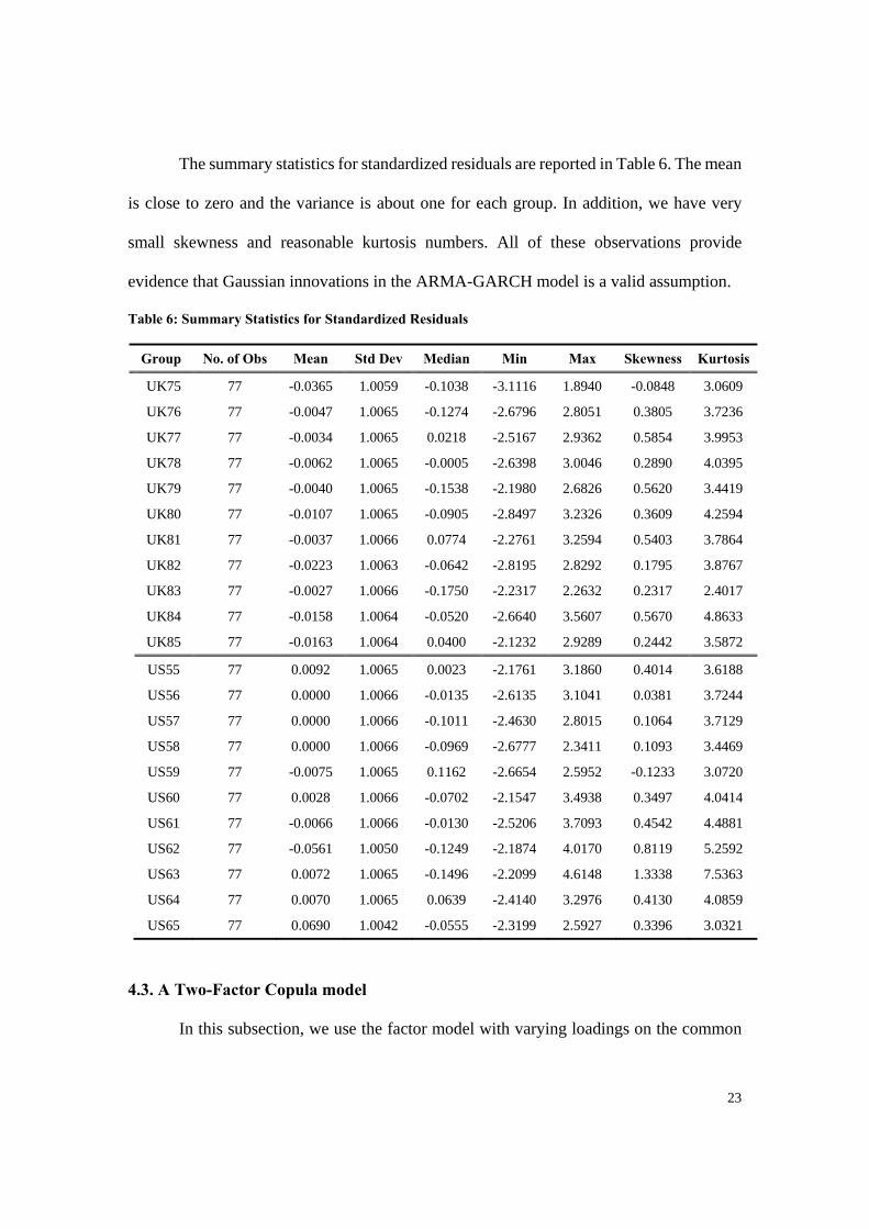
The summary statistics for standardized residuals are reported in Table 6. The mean
is close to zero and the variance is about one for each group. In addition, we have very
small skewness and reasonable kurtosis numbers. All of these observations provide
evidence that Gaussian innovations in the ARMA-GARCH model is a valid assumption.
Table 6: Summary Statistics for Standardized Residuals
Group No. of Obs Mean Std Dev Median Min Max Skewness Kurtosis
UK75 77 -0.0365 1.0059 -0.1038 -3.1116 1.8940 -0.0848 3.0609
UK76 77 -0.0047 1.0065 -0.1274 -2.6796 2.8051 0.3805 3.7236
UK77 77 -0.0034 1.0065 0.0218 -2.5167 2.9362 0.5854 3.9953
UK78 77 -0.0062 1.0065 -0.0005 -2.6398 3.0046 0.2890 4.0395
UK79 77 -0.0040 1.0065 -0.1538 -2.1980 2.6826 0.5620 3.4419
UK80 77 -0.0107 1.0065 -0.0905 -2.8497 3.2326 0.3609 4.2594
UK81 77 -0.0037 1.0066 0.0774 -2.2761 3.2594 0.5403 3.7864
UK82 77 -0.0223 1.0063 -0.0642 -2.8195 2.8292 0.1795 3.8767
UK83 77 -0.0027 1.0066 -0.1750 -2.2317 2.2632 0.2317 2.4017
UK84 77 -0.0158 1.0064 -0.0520 -2.6640 3.5607 0.5670 4.8633
UK85 77 -0.0163 1.0064 0.0400 -2.1232 2.9289 0.2442 3.5872
US55 77 0.0092 1.0065 0.0023 -2.1761 3.1860 0.4014 3.6188
US56 77 0.0000 1.0066 -0.0135 -2.6135 3.1041 0.0381 3.7244
US57 77 0.0000 1.0066 -0.1011 -2.4630 2.8015 0.1064 3.7129
US58 77 0.0000 1.0066 -0.0969 -2.6777 2.3411 0.1093 3.4469
US59 77 -0.0075 1.0065 0.1162 -2.6654 2.5952 -0.1233 3.0720
US60 77 0.0028 1.0066 -0.0702 -2.1547 3.4938 0.3497 4.0414
US61 77 -0.0066 1.0066 -0.0130 -2.5206 3.7093 0.4542 4.4881
US62 77 -0.0561 1.0050 -0.1249 -2.1874 4.0170 0.8119 5.2592
US63 77 0.0072 1.0065 -0.1496 -2.2099 4.6148 1.3338 7.5363
US64 77 0.0070 1.0065 0.0639 -2.4140 3.2976 0.4130 4.0859
US65 77 0.0690 1.0042 -0.0555 -2.3199 2.5927 0.3396 3.0321
4.3. A Two-Factor Copula model
In this subsection, we use the factor model with varying loadings on the common
24
factor. Based on the distribution assumptions for the factors, we consider 4 models: Student
t - Normal, Student t - Student t, Skewed t - Normal and Skewed t - Student t. For example,
in the Skewed t - Normal factor copula model, we assume that the common factor 0Z
follows a skewed t distribution with two shape parameters: a skewness parameter,
( 1,1) , which controls for the degree of asymmetry, and a degree of freedom parameter,
(2, ) , which controls the thickness of the tails. We assume that the country factor cZ
and the idiosyncratic factor follow a normal distribution with mean 0 and variance 2 .
We further assume that they are all independent.
To implement the SMM estimator of the copula models, we have to choose
dependence measures as our “moments”. We use pair-wise Spearman’s rho and quantile
dependence with q = [0.25, 0.75]. Those measures are “pure” measures of dependence,
meaning that they are solely affected by the changes in the copula, not by the changes in
the marginal distribution. For a detailed discussion of such “pure” dependence measures,
see Joe (1997) and Nelsen (2006).
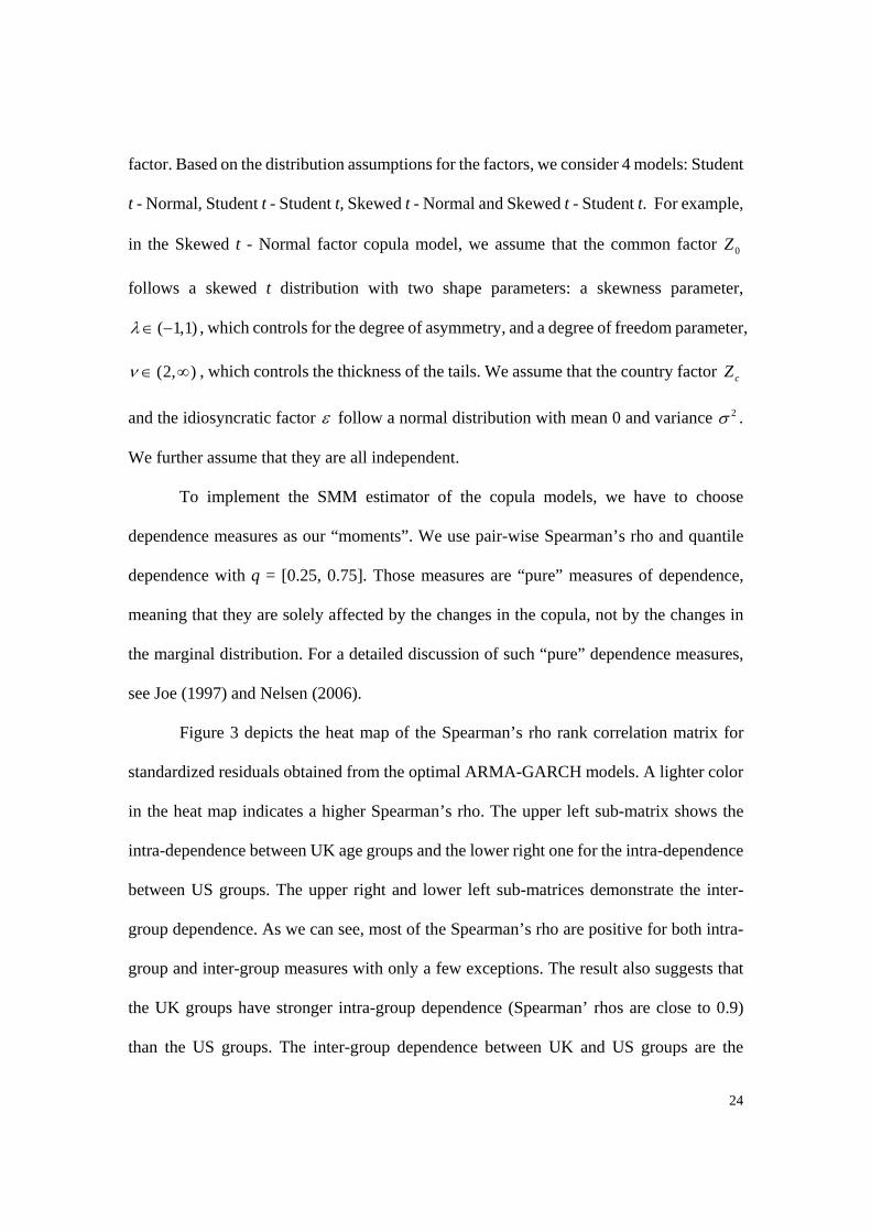
Figure 3 depicts the heat map of the Spearman’s rho rank correlation matrix for
standardized residuals obtained from the optimal ARMA-GARCH models. A lighter color
in the heat map indicates a higher Spearman’s rho. The upper left sub-matrix shows the
intra-dependence between UK age groups and the lower right one for the intra-dependence
between US groups. The upper right and lower left sub-matrices demonstrate the inter-
group dependence. As we can see, most of the Spearman’s rho are positive for both intra-
group and inter-group measures with only a few exceptions. The result also suggests that
the UK groups have stronger intra-group dependence (Spearman’ rhos are close to 0.9)
than the US groups. The inter-group dependence between UK and US groups are the
25
weakest. We calculate the p-value for the Spearman’s rho. We find that all intra-group
dependence measures are highly significant at the 5% level while the inter-group
dependence measures are almost insignificant.
Figure 3: Heatmap for Spearman rank correlation matrix
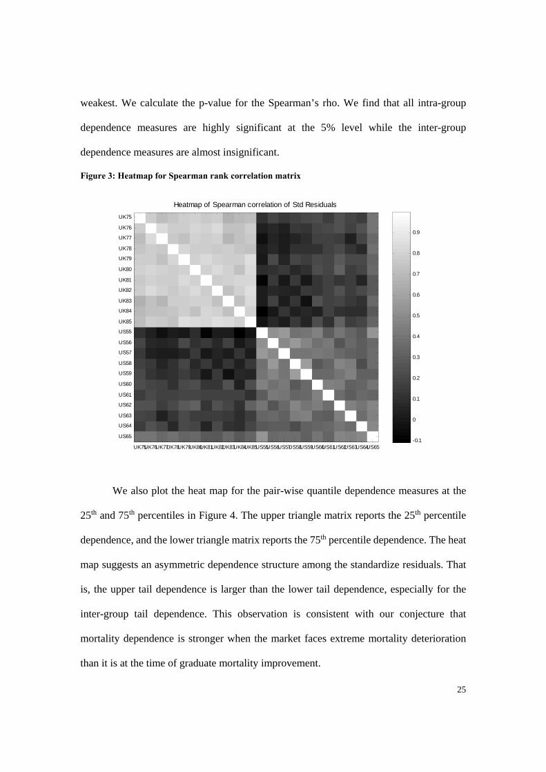
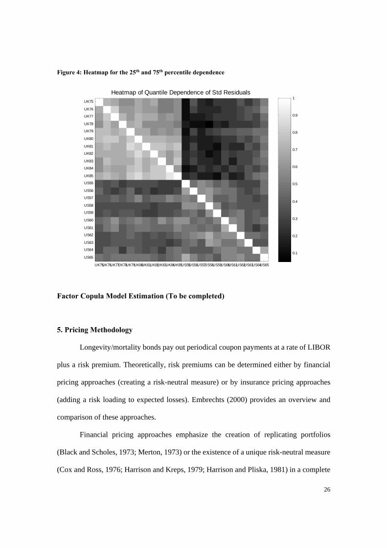
We also plot the heat map for the pair-wise quantile dependence measures at the
25th and 75th percentiles in Figure 4. The upper triangle matrix reports the 25th percentile
dependence, and the lower triangle matrix reports the 75th percentile dependence. The heat
map suggests an asymmetric dependence structure among the standardize residuals. That
is, the upper tail dependence is larger than the lower tail dependence, especially for the
inter-group tail dependence. This observation is consistent with our conjecture that
mortality dependence is stronger when the market faces extreme mortality deterioration
than it is at the time of graduate mortality improvement.
Heatmap of Spearman correlation of Std Residuals
UK75UK76UK77UK78UK79UK80UK81UK82UK83UK84UK85US55US56US57US58US59US60US61US62US63US64US65
UK75
UK76
UK77
UK78
UK79
UK80
UK81
UK82
UK83
UK84
UK85
US55
US56
US57
US58
US59
US60
US61
US62
US63
US64
US65-0.1
0
0.1
0.2
0.3
0.4
0.5
0.6
0.7
0.8
0.9
26
Figure 4: Heatmap for the 25th and 75th percentile dependence
Factor Copula Model Estimation (To be completed)
5. Pricing Methodology
Longevity/mortality bonds pay out periodical coupon payments at a rate of LIBOR
plus a risk premium. Theoretically, risk premiums can be determined either by financial
pricing approaches (creating a risk-neutral measure) or by insurance pricing approaches
(adding a risk loading to expected losses). Embrechts (2000) provides an overview and
comparison of these approaches.
Financial pricing approaches emphasize the creation of replicating portfolios
(Black and Scholes, 1973; Merton, 1973) or the existence of a unique risk-neutral measure
(Cox and Ross, 1976; Harrison and Kreps, 1979; Harrison and Pliska, 1981) in a complete
Heatmap of Quantile Dependence of Std Residuals
UK75UK76UK77UK78UK79UK80UK81UK82UK83UK84UK85US55US56US57US58US59US60US61US62US63US64US65
UK75
UK76
UK77
UK78
UK79
UK80
UK81
UK82
UK83
UK84
UK85
US55
US56
US57
US58
US59
US60
US61
US62
US63
US64
US650.1
0.2
0.3
0.4
0.5
0.6
0.7
0.8
0.9
1

27
market. In an incomplete market (e.g., the mortality/longevity market), with sparse market
price data some prevalent pricing methodologies, such as the arbitrage free pricing method
(Cairns et al. 2006, Bauer et al. 2010), the Wang transform (Dowd et al. 2006, Denuit et al.
2007, Lin and Cox 2008, Chen and Cox 2009), or the Esscher transform (Chen et al. 2010,
Li et al. 2010), often require the user to make one or more subjective assumptions to derive
the market prices of risk. The pricing process becomes even more difficult when multiple
risks are involved.
The alternative insurance pricing approaches usually assume investors are risk
averse, thereby adding a risk loading to the expected loss to compensate investors for the
risk of the insurance contract. The risk loading is either proportional to the expected loss
(EL), or to the variance or standard deviation of the loss, or determined by a Cobb–Douglas
function on the probability of first loss (PFL) and the conditional expected loss (CEL)
(Lane 2000). Extending the previous work, Lane and Beckwith (2008) and Lane and Mahul
(2008) suggest a multiple linear model using the expected loss and a factor covering cycle
effects to decide risk premiums. Other multiple linear approaches have been established by
Berge (2005) and Dieckmann (2008). Both analyses identify Cat-bond-specific factors,
such as peril, trigger, size, and rating, to capture the risk loading. Loglinear models have
also been used in Major and Kreps (2003) and Dieckmann (2008).
The model that we propose to use in this paper can be written as follows
ln Premium ln lnPFL CEL Z
We use the following explanatory variables in our model.
Risk Measures. In a perfect, riskless market, the risk premium should be equal to
the expected loss, provided that insurance risk is uncorrelated with the movement of

28
financial markets. However, insurance markets are not riskless and are far from perfect.
Therefore, investors normally require a risk loading to compensate for risk bearing in the
market for catastrophe securities (Lane, 2000). The expected loss principle sets the risk
loading proportional to the expected loss. It requires only the first moment of the loss
distribution and thus can be easily implemented. It, however, is not risk sensitive. The
variance/standard deviation principle takes into account the variation of the risk and works
well for symmetric random outcomes. However, insurance risk is often skewed: most of
the probability mass is centered at zero loss, while there is a small probability of potentially
large negative returns. Lane (2000) use the conditional expected loss (CEL) to measure the
loss severity (and capture the asymmetry of insurance risk) and the probability of first loss
(PFL) to measure the loss frequency in a risk cubic pricing model. We include EL, CEL
and PFL in our model.
Trigger. The payout of a CAT bond depends on trigger mechanisms. Basically,
there are five different trigger mechanisms: indemnity, modelled loss, industry loss,
parametric or hybrid triggers. Cummins and Weiss (2009) and Dubinsky and Laster (2003)
argue that CAT bond prices with an indemnity trigger might be higher than those with other
triggers due to moral hazard. They also state that transaction costs for indemnity triggered
CAT bonds are very high, because more documentation is needed compared to
nonindemnity trigger mechanisms. For this purpose, we include a dummy variable
Indemnity whose value is equal to one if the CAT bond is indemnity triggered and zero
otherwise.
Rating. Investors usually require credit risk premiums for corporate bonds because
of bearing credit risk. For CAT bonds, a rating has been assigned by at least one of the
29
three rating agencies S&P, Moodys, or Fitch. To test whether the CAT bond rating plays a
role in its premium pricing, we include a dummy variable BBB+ to indicate a CAT bond
with a BBB or A rating, and a dummy variable BB for a CAT bond with a BB rating. CAT
bonds with a rating lower than BB are omitted.
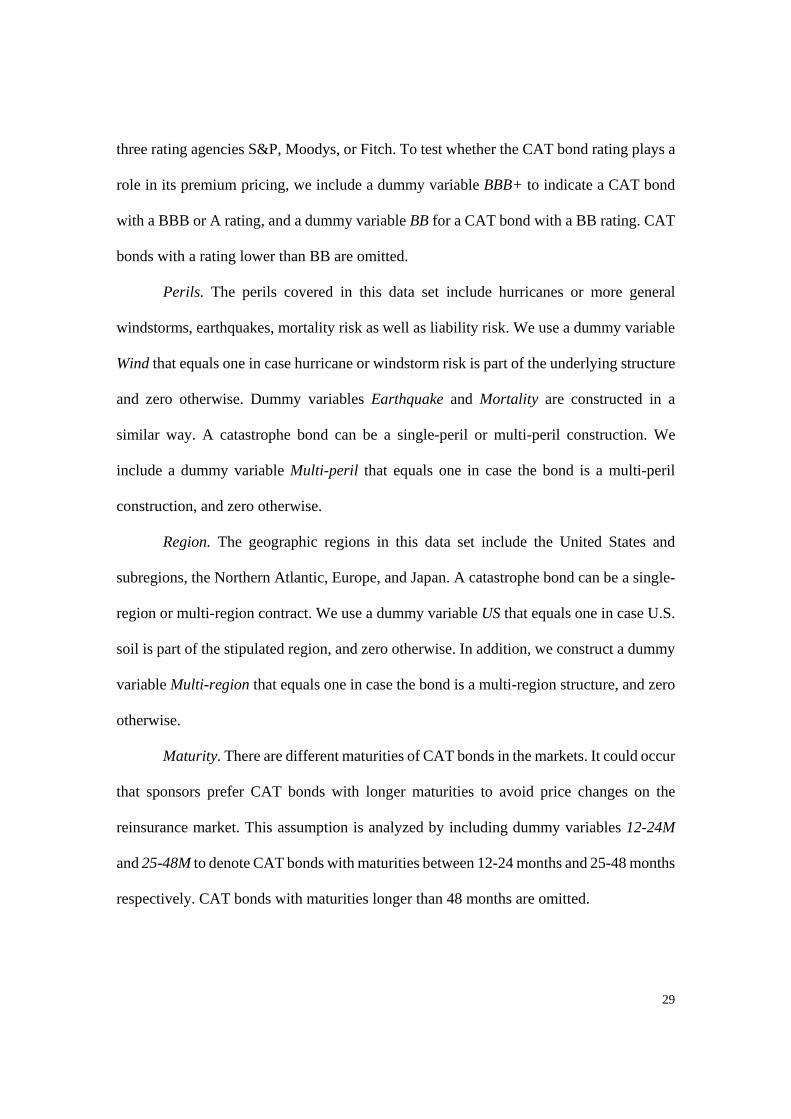
Perils. The perils covered in this data set include hurricanes or more general
windstorms, earthquakes, mortality risk as well as liability risk. We use a dummy variable
Wind that equals one in case hurricane or windstorm risk is part of the underlying structure
and zero otherwise. Dummy variables Earthquake and Mortality are constructed in a
similar way. A catastrophe bond can be a single-peril or multi-peril construction. We
include a dummy variable Multi-peril that equals one in case the bond is a multi-peril
construction, and zero otherwise.
Region. The geographic regions in this data set include the United States and
subregions, the Northern Atlantic, Europe, and Japan. A catastrophe bond can be a single-
region or multi-region contract. We use a dummy variable US that equals one in case U.S.
soil is part of the stipulated region, and zero otherwise. In addition, we construct a dummy
variable Multi-region that equals one in case the bond is a multi-region structure, and zero
otherwise.
Maturity. There are different maturities of CAT bonds in the markets. It could occur
that sponsors prefer CAT bonds with longer maturities to avoid price changes on the
reinsurance market. This assumption is analyzed by including dummy variables 12-24M
and 25-48M to denote CAT bonds with maturities between 12-24 months and 25-48 months
respectively. CAT bonds with maturities longer than 48 months are omitted.
30
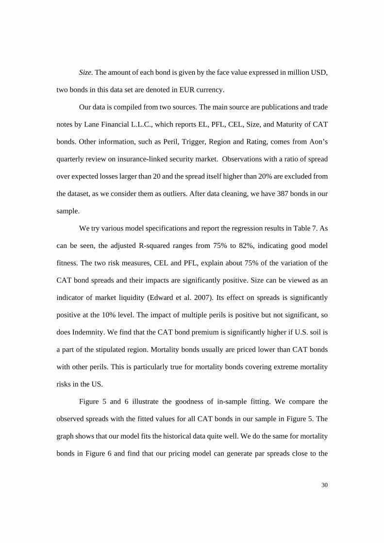
Size. The amount of each bond is given by the face value expressed in million USD,
two bonds in this data set are denoted in EUR currency.
Our data is compiled from two sources. The main source are publications and trade
notes by Lane Financial L.L.C., which reports EL, PFL, CEL, Size, and Maturity of CAT
bonds. Other information, such as Peril, Trigger, Region and Rating, comes from Aon’s
quarterly review on insurance-linked security market. Observations with a ratio of spread
over expected losses larger than 20 and the spread itself higher than 20% are excluded from
the dataset, as we consider them as outliers. After data cleaning, we have 387 bonds in our
sample.
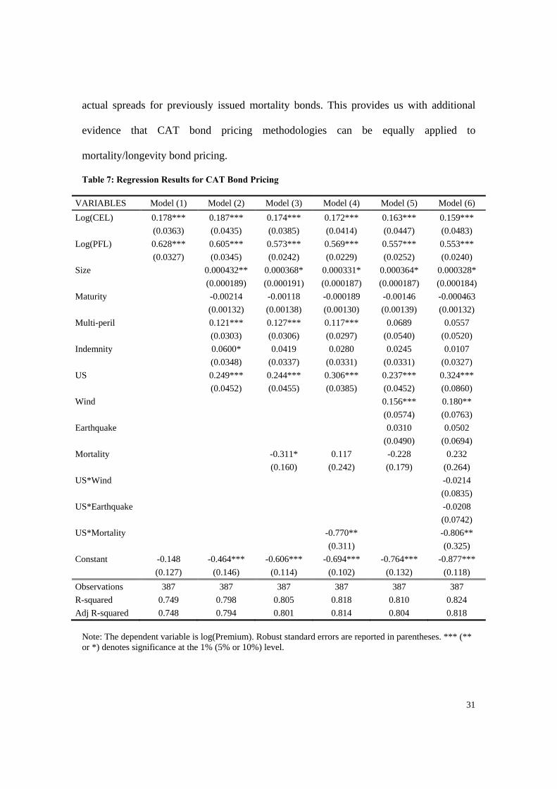
We try various model specifications and report the regression results in Table 7. As
can be seen, the adjusted R-squared ranges from 75% to 82%, indicating good model
fitness. The two risk measures, CEL and PFL, explain about 75% of the variation of the
CAT bond spreads and their impacts are significantly positive. Size can be viewed as an
indicator of market liquidity (Edward et al. 2007). Its effect on spreads is significantly
positive at the 10% level. The impact of multiple perils is positive but not significant, so
does Indemnity. We find that the CAT bond premium is significantly higher if U.S. soil is
a part of the stipulated region. Mortality bonds usually are priced lower than CAT bonds
with other perils. This is particularly true for mortality bonds covering extreme mortality
risks in the US.
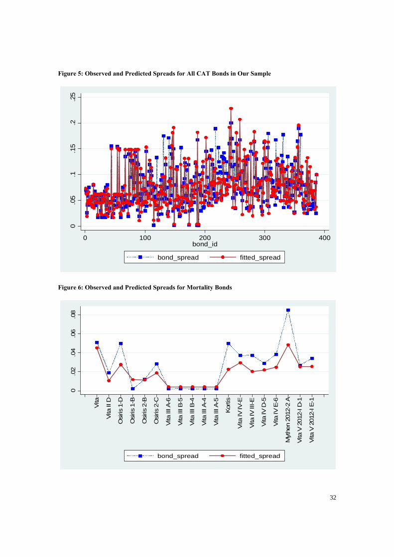
Figure 5 and 6 illustrate the goodness of in-sample fitting. We compare the
observed spreads with the fitted values for all CAT bonds in our sample in Figure 5. The
graph shows that our model fits the historical data quite well. We do the same for mortality
bonds in Figure 6 and find that our pricing model can generate par spreads close to the
31
actual spreads for previously issued mortality bonds. This provides us with additional
evidence that CAT bond pricing methodologies can be equally applied to
mortality/longevity bond pricing.
Table 7: Regression Results for CAT Bond Pricing
VARIABLES Model (1) Model (2) Model (3) Model (4) Model (5) Model (6)
Log(CEL) 0.178*** 0.187*** 0.174*** 0.172*** 0.163*** 0.159***
(0.0363) (0.0435) (0.0385) (0.0414) (0.0447) (0.0483)
Log(PFL) 0.628*** 0.605*** 0.573*** 0.569*** 0.557*** 0.553***
(0.0327) (0.0345) (0.0242) (0.0229) (0.0252) (0.0240)
Size 0.000432** 0.000368* 0.000331* 0.000364* 0.000328*
(0.000189) (0.000191) (0.000187) (0.000187) (0.000184)
Maturity -0.00214 -0.00118 -0.000189 -0.00146 -0.000463
(0.00132) (0.00138) (0.00130) (0.00139) (0.00132)
Multi-peril 0.121*** 0.127*** 0.117*** 0.0689 0.0557
(0.0303) (0.0306) (0.0297) (0.0540) (0.0520)
Indemnity 0.0600* 0.0419 0.0280 0.0245 0.0107
(0.0348) (0.0337) (0.0331) (0.0331) (0.0327)
US 0.249*** 0.244*** 0.306*** 0.237*** 0.324***
(0.0452) (0.0455) (0.0385) (0.0452) (0.0860)
Wind 0.156*** 0.180**
(0.0574) (0.0763)
Earthquake 0.0310 0.0502
(0.0490) (0.0694)
Mortality -0.311* 0.117 -0.228 0.232
(0.160) (0.242) (0.179) (0.264)
US*Wind -0.0214
(0.0835)
US*Earthquake -0.0208
(0.0742)
US*Mortality -0.770** -0.806**
(0.311) (0.325)
Constant -0.148 -0.464*** -0.606*** -0.694*** -0.764*** -0.877***
(0.127) (0.146) (0.114) (0.102) (0.132) (0.118)
Observations 387 387 387 387 387 387
R-squared 0.749 0.798 0.805 0.818 0.810 0.824
Adj R-squared 0.748 0.794 0.801 0.814 0.804 0.818
Note: The dependent variable is log(Premium). Robust standard errors are reported in parentheses. *** (** or *) denotes significance at the 1% (5% or 10%) level.
32
Figure 5: Observed and Predicted Spreads for All CAT Bonds in Our Sample
Figure 6: Observed and Predicted Spreads for Mortality Bonds
0.0
5.1
.15
.2.2
5
0 100 200 300 400bond_id
bond_spread fitted_spread
0.0
2.0
4.0
6.0
8
Vita
Vita
II D
Osi
ris
1-D
Osi
ris
1-B
Osi
ris
2-B
Osi
ris
2-C
Vita
III A
-6
Vita
III B
-5
Vita
III B
-4
Vita
III A
-4
Vita
III A
-5
Kor
tis
Vita
IV IV
-E
Vita
IV II
I-E
Vita
IV D
-5
Vita
IV E
-6
Myt
hen
2012
-2 A
Vita
V 2
012
-I D
-1
Vita
V 2
012
-I E
-1
bond_spread fitted_spread

33
6. Conclusions
Many life insurers and reinsurers operate internationally and pool policies across
countries. It is, therefore, increasingly important for them to understand the joint mortality
dynamics for multiple populations and assess mortality/longevity risk in their own books
of business. To hedge the risk, they actively participate in mortality/longevity
securitizations and engage in issuing or trading mortality-linked securities. The reference
populations associated with these hedging instruments usually exhibit mortality
improvement rates that are different from those of the hedger’s population and this
introduces basis risk that the hedger must manage. In addition, almost all mortality
securitizations, albeit their difference in structure, have payoffs contingent on a weighted
mortality index of multiple populations. Therefore, developing mortality models for
multiple populations and understanding the correlated mortality risks are crucial to life
insurers and pension planners.
Although there is a rich literature for mortality modeling in a single population,
only a few papers (see, e.g., the reference cited in introduction) examine two-population
mortality models. These models are based on a critical assumption that mortality rates of
two populations do not diverge in the long run, which seems too strong for short-term
mortality forecasts. In spite of the extensive use of copula models in finance and economics,
only two studies (i.e., Chen et al. 2013 and Wang et al. 2013) has explored its application
to multi-population mortality analysis.
In this paper, we propose a dynamic multivariate mortality model based on a factor
copula and the GAS structure. The factor copula model that we use has a simple (additive)
form and is flexible in model specification according to data availability and the number
of variables that need to be specified. It is particularly useful to high dimension application.
34
This characteristic is important when the number of populations that we need to model is
large. We extend the one-factor model in Chen et al. (2013) to a two-factor copula model,
with one factor representing the common, market force and the other having a country-
specific mortality effect. We also introduce dynamic dependence among multiple
populations using the GAS structure.
Finally, we illustrate how to apply our model to modeling risk modelling and
pricing. Using the Kortis bond as one example, we fit the mortality model for US male 55-
65 and UL male 75-85 and project the probability of the bond principal reduction. We
apply the CAT bond empirical pricing methodology to mortality/longevity bond pricing.
Our regression model can explain about 80% of the premium variations for CAT bonds.
When examining mortality/longevity bonds only, we find the fitted par spreads are very
close to the premiums observed on the primary market.

35
Reference: Bauer, D., M. Boerger, and J. Russ (2010). On the pricing of longevity-linked securities,
Insurance: Mathematics and Economics 46(1): 139-149. Berge, T. (2005). Katastrophenanleihen. Anwendung, Bewertung,
estaltungsempfehlungen (Lohmar: EUL Verlag). Black, F. and M. Scholes (1973). The pricing of options and corporate liabilities, Journal
of Political Economy 81 (3): 637–654. Box, G. E. P., and G. M. Jenkins (1976). Time Series Analysis: Forecasting and Control,
2nd ed. San Francisco: Holden-Day. Cairns, A. J. G., D. Blake, and K. Dowd (2006). A Two-factor model for stochastic
mortality with parameter uncertainty: Theory and calibration, Journal of Risk and Insurance 73(4): 687-718.
Cairns, A. J. G., Blake, D., Dowd, K., Coughlan, G. D., and Khalaf-Allah, M. (2011) Bayesian Stochastic Mortality Modelling for Two Populations. ASTIN Bulletin 41: 29-59.
Carriere, J. F. (2000). Bivariate survival models for coupled lives. Scandinavian Actuarial Journal 1: 17–31.
Chen, H., and S. H. Cox (2009). Modeling mortality with jumps: Applications to mortality securitization, Journal of Risk and Insurance 76(3): 727-751.
Chen, H., S. H. Cox, and S. S. Wang (2010). Is the Home Equity Conversion Program in the United States sustainable? Evidence from pricing mortgage insurance premiums and Non-Recourse Provisions using the conditional Esscher transform, Insurance: Mathematics and Economics 46(2): 371-384.
Chen, H. and D. J. Cummins (2010). Longevity bond premiums: the extreme value approach and risk cubic pricing, Insurance: Mathematics and Economics 46(1): 150-161.
Chen, H., R. MacMinn and T. Sun (2013). Multi-population Mortality Models: A Factor Copula Approach, working paper, Temple University.
Cox, C. J. and S. A. Ross (1976). The valuation of options for alternative stochastic processes,Journal of Financial Economics, 3(1-2):145-166.
Creal, D.D., S.J. Koopman, and A. Lucas (2013). Generalized autoregressive score Models with Applications, Journal of Applied Econometrics 28(5):777-795.
Cummins, J. D. and M. A. Weiss (2009). Convergence of insurance and financial markets: hybrid and securitized risk transfer solutions, Journal of Risk and Insurance 76(3) 493-545.
Denuit, M., P. Devolder, and A. C. Goderniaux (2007). Securitization of longevity risk: Pricing survivor bonds with Wang Transform in the Lee–Carter framework, Journal of Risk and Insurance 74(1): 87-113.
Denuit, M., J. Dhaene, C., Le Bailly de Tilleghem, and S. Teghem (2001). Measuring the impact of dependence among insured lifelengths. Belgian Actuarial Bulletin, 1(1): 18–39.
Dieckmann, S. (2008). By force of nature: explaining the yield spread on catastrophe bonds, Working Paper, Wharton School, University of Pennsylvania, Philadelphia, PA.
Dowd, K., D. Blake, A. J. G. Cairns, and P. Dawson (2006). Survivor swaps, Journal of Risk and Insurance 73(1): 1-17.

36
Dowd, K., A. J. G. Cairns, D. Blake, G. D. Coughlan and M. Khalaf-Allah (2011). A gravity model of mortality rates for two related populations. North American Actuarial Journal 15(2): 334-356.
Dubinsky, W., and D. Laster (2003). Insurance-Linked Securities, Swiss Re Capital Markets Corporation.
Embrechts, P. (2000). Actuarial vs financial pricing of insurance, unpublished manuscript. Embrechts, P., F. Lindskog, and A. McNeil (2003). Modeling dependence with copulas
and applications to risk management In: Handbook of Heavy Tailed Distributions in Finance, ed. S. Rachev, Elsevier, Chapter 8, 329-384.
Engle, R.F. (2002). Dynamic conditional correlation: A simple class of multivariate generalized autoregressive conditional heteroskedasticity models, Journal of Business & Economic Statistics 20(3): 339-350.
Frees, E. W., J. F. Carriere, and E. A. Valdez (1996). Annuity valuation with dependent mortality. Journal of Risk and Insurance 63 (2), 229–261.
Frees, E. W., and E. A. Valdez (1998). Understanding relationships using copula, North American Actuarial Journal 2(1): 1-25.
Hafner, C.M. and H. Manner (2012). Dynamic stochastic copula models: estimation, inference and applications, Journal of Applied Econometrics 27(2):269-295.
Harrison, J. M. and D. M. Kreps (1979). Martingales and arbitrage in multiperiod securities markets, Journal of Economic Theory 20(3): 381-408.
Harrison, J.M. and S. R. Pliska (1981). Martingales and Stochastic integrals in the theory of continuous trading, Stochastic Processes and their Applications 11 (3): 215–260.
Hunt,A., and D. Blake (2013). Modelling longevity bonds: Analysing the Swiss Re Kortis Bond, working paper, Pension Institute.Jarner, S. F. and E. M. Kryger (2011). Modelling adult mortality in small populations: the SAINT model. ASTIN Bulletin 41: 377-418.
Joe, H. (1997). Multivariate models and dependence concepts, Monographs in Statistics and Probability 73, Chapman and Hall, London.
Joe, H. (2005). Asymptotic efficiency of the two-stage estimation method for copula-based models, Journal of Multivariate Analysis 94: 401-419
Lane, M. N. and O. Y. Movchan (1999). Risk cubes or price risk and rating (part II), Journal of Risk Finance 1(1): 71-86.
Lane, M. N.(2000). Pricing risk transfer transactions, ASTIN Bulletin 30(2): 259-293. Lane, M. N., and R. G. Beckwith (2008). The 2008 Review of ILS Transactions—What
Price ILS? A Work in Progress. Lane Financial LLC Trade Notes, March 31. Lane, M. N., and O. Mahul (2008). Catastrophe Risk Pricing: An Empirical Analysis,
Policy Research Working Paper 4765, The World Bank. Lee, R.D., and L. R. Carter (1992). Modeling and forecasting U.S. mortality. Journal of
the American Statistical Association 87: 659-671. Li, N., and R. Lee (2005). Coherent mortality forecasts for a group of population: An
extension to the classical Lee-Carter Approach. Demography 42: 575-594. Li, J. S.-H. (2010). Pricing longevity risk with the parametric bootstrap: A maximum
entropy approach, Insurance: Mathematics and Economics 47(2):176-186. Li, J. S.-H. and M. R. Hardy (2011). Measuring basis risk in longevity hedges, North
American Actuarial Journal 15(2): 177-200.
37
Li, J. S.-H., M. R. Hardy, and K. S. Tan (2010). Pricing and hedging the no-negative-equity-guarantee in equity release mechanisms, Journal of Risk and Insurance 77(2):499-522.
Lin, Y., and S. H. Cox (2008). Securitization of catastrophe mortality risks, Insurance: Mathematics and Economics 42(2): 628-637.
Lin, Y., S. Liu and J. Yu (2013). Pricing mortality securities with correlated mortality indexes, Journal of Risk and Insurance 80 (4): 921-948.
Manner, H. and J. Segers (2011). Tails of correlation mixtures of elliptical copulas, Insurance: Mathematics and Economics 48(1): 153-160.
Major, J., and R. Kreps (2003). Catastrophe risk pricing in the traditional market, in: M. Lane, ed., Alternative Risk Strategies (London: Risk Books).
Merton, C. R., (1973). Theory of rational option pricing, Bell Journal of Economics and Management Science 4(1): 141-183.
Nelsen, R. B. (2006). An Introduction to Copulas, Second Edition, Springer, U.S.A Patton, A. J. (2006). Estimation of multivariate models for time series of possibly different
lengths, Journal of Applied Econometrics 21(2): 147-173. Oh, D. H., and A. J. Patton (2012). Modelling dependence in high dimensions with factor
copulas, working paper, Duke University. Oh, D. H., and A. J. Patton (2013). Time-varying systemic risk: evidence from a dynamic
copula model of CDS spreads, working paper, Duke University. Shephard, N., 2005, Stochastic Volatility: Selected Readings, Oxford University Press,
Oxford. Shemyakin, A. and H. Youn (2006). Copula models of joint last survivor analysis. Applied
Stochastic Models in Business and Industry, 22: 211–224. Swiss Re (2012). A mature market: building a capital market for longevity risk. Swiss Re
Europe S.A., UK branch. Wang, C. W., S. S. Yang, and H. C. Huang (2013). Modelling multi-coungry mortality
dependence and its application in pricing survivor index swaps-a dynamic copula approach, working paper.
Yang, S. S. and C.-W Wang (2013). Pricing and securitization of multi-country longevity risk with mortality dependence, Insurance: Mathematics and Economics 52(2):157-169.
Youn, H. and A. Shemyakin (1999). Statistical aspects of joint life insurance pricing. 1999 Proceedings of the Business and Statistics Section of the American Statistical Association, 34–38.
Youn, H. and A. Shemyakin (2001). Pricing practices for joint last survivor insurance. Actuarial Research Clearing House, 2001.1.
Zhou, R., J. S.-H. Li and K. S. Tan (2013a) Pricing standardized mortality securitizations: A two-population model with transitory jump effects, Journal of Risk and Insurance 80(3): 733-774.
Zhou, R., Y. Wang, K, Kaufhold, J. S.-H. Li and K. S. Tan (2013b). Modeling mortality of multiple populations with vector error correction models: Applications to solvency II, working paper.