Embed Size (px)
Citation preview
Mortality Change, the Uncertainty Effect, and Retirement ∗
Sebnem Kalemli-OzcanUniversity of Houston and NBER
David N. WeilBrown University and NBER
February 6, 2010
Abstract
We examine the role of declining mortality in explaining the rise of retirement over the course of the20th century. We construct a model in which individuals make labor/leisure choices over their lifetimessubject to uncertainty about their dates of death. In an environment with high mortality, an individualwho saves for retirement faces a high risk of dying before he can enjoy his planned leisure. In this case,the optimal plan is for people to work until they die. As mortality falls, however, it becomes optimalto plan, and save for, retirement. We analyze our model using two mathematical formulations of thesurvival function as well as data on actual changes in the US life table over the last century, and show thatthis “uncertainty effect” of declining mortality would have more than outweighed the “horizon effect” bywhich rising life expectancy would have led to later retirement.
JEL Classification: E21, I12, J11, J26
∗We thank Andrew Foster, Herschel Grossman, Chinhui Juhn, Robin Lumsdaine, Enrico Spolaore, and seminar participantsat The Bank of Israel, Bar-Ilan University, Ben-Gurion University, Bilkent University, Brown University, Hebrew University,University of Houston, Koc University, University of Maryland, Rice University, University of Rochester, Tel Aviv University,and the Harvard School of Public Health Conference on Population Aging and Economic Growth for helpful comments. We areparticularly grateful to Omar Licandro, who refereed the paper for the Journal of Economic Growth. His report, which wasanonymous until after the paper was accepted, served as the basis for major improvements in our results and their presentation.Isabel Tecu provided superlative research assistance.
1
1 Introduction
One of the most dramatic economic changes in the last 100 years has been the rise in retirement as an
important stage of life. At the beginning of the twentieth century, retirement was a rarity. Many people
didn’t live into old age, and most of those who did continued to work until shortly before death. By the end
of the century, the vast majority of workers could expect to experience a prolonged period of healthy leisure
after their working years were over.
Needless to say, the economic repercussions of this change in the life cycle pattern of labor supply have
been enormous. Since a significant fraction of consumption during retirement is publicly funded, the growth
in retirement has strained government budgets - a phenomenon which will soon be exacerbated by population
aging (Weil, 2008). Meanwhile, private funding of anticipated retirements has led to the accumulation of
vast pools of capital. Exactly what fraction of current capital accumulation can be attributed to life cycle
savings is an issue of contentious debate. Modigliani’s (1988) estimate is that as much as 80% of wealth
can be attributed to life cycle saving, while Kotlikoff and Summers (1988) estimate that it is only 20%.
According to Lee (2001), the fraction of wealth attributable to life cycle saving in the US doubled between
1900 and 1990.
Explaining the rise in retirement has been a major endeavor for economists in the last several decades.
Three prominent explanations can be discerned. The first is that public pension programs, such as Social
Security in the United States, have been instrumental in pushing workers out of the labor force, particularly
through high implicit rates of taxation on wage income earned at older ages (Gruber and Wise, 1998). The
second explanation is that rising lifetime income has led workers to optimally choose a larger period of leisure
at the end of life (Costa, 1998). The final explanation is that changes in the technology of production have
lowered the productivity of older workers, leading employers to seek to get rid of them (Graebner, 1980;
Sala-i-Martin, 1996). None of these explanations, either taken separately or as a group, has been completely
successful in accounting for the rise in retirement. This paper proposes a new explanation, which we call the
“uncertainty effect,” for the rise in retirement. Our explanation is not meant to be a complete substitute for
the factors discussed above, but rather an addition to the set of usual suspects that must be considered in
explaining the rise of retirement.
In our model, the driving force behind the change in the life-cycle pattern of labor supply is a change in
the pattern of mortality. Individuals make labor/leisure choices over their lifetimes subject to uncertainty
about their dates of death. In an environment in which uncertainty surrounding the date of death is high,
an individual who saved up for retirement would face a high risk of dying before he could enjoy his planned
2
leisure. In this case, the optimal plan is for individuals to work until they die. As uncertainty regarding
the date of death falls, individuals will find it optimal to plan, and save for, retirement. As we show below,
a salient feature of changes in mortality that have occurred in developed world over the last century is
that as life expectancy has risen, uncertainty regarding the date of death has fallen. The effect of falling
mortality on labor supply complements several other effects of falling mortality, most notably on human
capital investment and fertility, that have been analyzed in recent literature.1
The rest of our paper is structured as follows. In section two, we briefly examine historical data on
mortality and retirement, and also discuss at greater length some of the other explanations for the rise of
retirement. Section three presents and solves our model of endogenous retirement. The different parts of that
section use three different formulations of the survival function: exponential, for mathematical simplicity;
a realistic formulation based on the work of Boucekkine, de la Croix, and Licandro (2002), which we can
solve analytically; and a numerical analysis based on actual data from US life tables. Our key result is that
in all these cases, increases in life expectancy can lead declines, in some cases discontinuous, in the age of
retirement. Section four looks at the paths of consumption and asset accumulation implied by the retirement
behavior studied in section three. Section five looks at the interaction between our new channel and one of
the existing explanations for the rise in retirement, specifically rising income. Section six concludes.
2 Historical Data
2.1 Mortality
Falling mortality has been one of the most significant aspects of the process of economic growth over the
last several centuries. Male life expectancy at birth in the United States rose from 40.2 in 1850 to 47.8 in
1900 and 75.2 in 2005. The most significant component of mortality decline has been the reduction in infant
and child deaths. Obviously, this aspect of the mortality decline is not related to the issues of retirement
saving that we discuss in this paper. Although the decline in adult mortality has not been quite as dramatic
as that for children, it has nevertheless been a significant part of the story of economic growth over the last
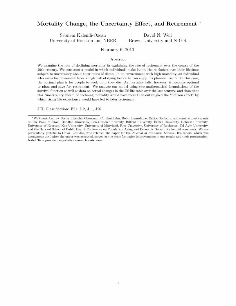
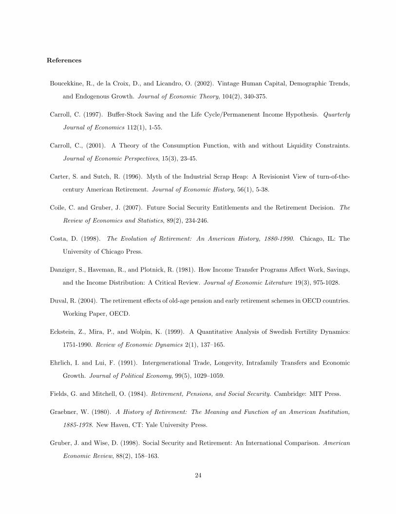
century or more. Figure 1 shows the number of survivors from a cohort of 20-year-olds who would be alive at
different ages, using life tables from the United States for 1850, 1900, 1950, and 2000, along with a forecast
for 2050. In 1850, the probability that a 20-year-old would reach age 65 was roughly 40%. By 2000, it was
roughly 80%. The total number of expected remaining years of life for a 20-year-old male rose from 38 to
1See Meltzer (1992), Ehrlich and Lui (1991), Eckstein et al. (1999), Kalemli-Ozcan (2003), and Hazan (forthcoming).
3
55 over this period.2
2.2 Retirement
Paralleling the reduction in male adult mortality has been a massive increase in retirement. In 1930, the
labor force participation rate for men aged 65 and over was 58%. By 1985, the rate had fallen to 16%, and has
since remained roughly constant.3 The trend in retirement prior to the Great Depression has been a subject
of controversy among historians. Ransom and Sutch (1986, 1988) claim that the labor force participation
rate for men over 60 was roughly constant between 1870 and 1930, while Costa (1998) and Moen (1994)
argue that labor force participation for older men had been declining since the late nineteenth century.
Examining the labor force participation of the elderly does not tell the full story, of course, because, as
shown above, a large fraction of the population never lived to this age. Carter and Sutch (1996) estimate
that at the beginning of the twentieth century, a 55-year-old man had only a 21.5% probability of retiring
before he died, excluding “death-bed retirement” associated with illness in the last weeks of life.
Another way to demonstrate the dramatic rise in retirement is to look at how the expected number of
years that an individual would spend retired has changed over time. This measure incorporates changes in
both mortality and labor force behavior. The expected period of retirement rose from 2.65 years (6.1% of
expected adult life) for the cohort born in 1830 to 5.50 years (11.6% of expected adult life) for the cohort
born in 1880 and 13.13 years (23.9% of expected adult life) for the cohort born in 1930 (Lee, 2001) Similarly,
Hazan (forthcoming) calculates that while life expectancy at age five rose from 52.5 years for men born in
1850 to 66.7 years for men born in 1930, expected years in the labor market only rose from 34.9 to 40.9 over
the same period.4
Although we focus our analysis on data from the United States, the rise of retirement has been universal
among developed countries. In the United Kingdom, for example, the labor force participation rate for men
aged 65 and over fell from 73.6% in 1881 to 58.9% in 1921, 18.6% in 1973, and 8.9% in 2003. In Japan, the
2Sources: Haines (1998), Keyfitz and Fleiger (1990). These are period rather than cohort life tables because the formerare available for a much longer period of time. We examine male mortality because the full-time labor force was dominatedby men in the age cohorts over which retirement rose to prominence. Further, prior to the rise of retirement, widows weregenerally supported by familial transfers rather than their own saving. For example, in 1940, only 18.4% of widows in the U.S.lived alone, while 58.7% lived with their adult children (McGarry and Schoeni, 2000). Looking at joint survival probabilitiespaints a picture similar to what is seen in male survival. Using the 1850 male and female life tables and assuming independencein mortality, the probability that a couple consisting of a 20 year old man and a 20 year old woman would have at least onemember survive to age 70 was 0.57; using the 2000 life table, the probability was 0.94.
3Such a change could theoretically be due to a changing age distribution of the population over 65 in the presence of constantage-specific participation rates. This is not the case, however: age specific participation rates have also fallen dramatically. SeeCosta (1998) and Lumsdaine and Wise (1994).
4Hazan also points out that because working hours per year declined over this period, the change in expected total workinghours over the lifetime was negative.
4
labor force participation rate for men aged 65-69 fell from 70% in 1960 to 47% in 2002. In France in the
four decades following 1960, male life expectancy rose from 67.6 to 74.2 while the average age of retirement
fell from 64.5 to 59.2.5
2.3 Explaining the Rise in Retirement
While we will argue that the decline in mortality is one explanation for the fall in labor force participation
of the elderly, it would be foolish to argue that it is the only one. Since we cannot incorporate all of these
effects into a single model, our approach will be to ask how large a change in retirement could plausibly be
explained by the mortality effect alone, in a model where the other factors are not present. In the rest of
this section, however, we briefly discuss three other channels.
The most obvious alternative explanation for the decline in labor force participation of the elderly is the
growth of public pension programs such as Social Security in the United States. The evidence regarding
how much of the rise in retirement is explained by public pension programs is mixed, but generally suggests
that such programs are not the dominant cause. Numerous studies find statistically significant effects of
Social Security on the likelihood or retiring at certain specific ages. For example, the hazard of retiring at
the “normal retirement age” of 65 was 20%, and the hazard of retiring at the first eligible age of 62 was
14%, in the United States in the 1990s. However, these studies generally imply a small impact of changes in
Social Security benefits on average age of retirement.6 Duval (2004), examining a panel of OECD countries,
finds that changes in public pension programs as well as other social programs such as unemployment and
disability insurance that are used as de facto early retirement schemes explain 31% of the decline in labor
force participation over the last three decades. Similarly, Johnson (2001), using a panel of data from 13
countries, finds that old age insurance explains only 11% of the drop in labor force participation by men
aged 60-64 over the period 1950-2000. By contrast, Gruber and Wise (1999), examining a cross section
of OECD countries, argue that differences in public pension provisions are the dominant explanation for
cross-country differences in labor force participation of men aged 55-64.
A second explanation for the rise in retirement focuses on the income effect of higher wages. In a taste-
based model of retirement, the association of higher income per capita with longer retirement comes about
because people in richer countries choose to spend a higher fraction of their income on retirement. When the
wage increases, there is an income effect, which leads to the purchase of more of all normal goods, including
leisure, and a substitution effect, which works to reduce leisure by raising its opportunity cost. For higher
5Gruber and Wise (1999), Matthews et al. (1982), Yashiro and Oshio (1999), Pestieau (2003), OECD (2004).6See Samwick (1998) and Coile and Gruber (2007) for a discussion.
5

income to lead to longer retirement, not only must the income effect dominate, but there must also be some
reason why this leisure must be taken at the end of life, rather than spread out evenly. The best argument
for this phenomenon is that there is some kind of non-convexity in the enjoyment of leisure; a simple example
would be that only people with full time leisure can move to Florida.7
A third explanation for the increase in retirement looks toward production technology. This explanation
starts with the notion that older workers are less able to do certain tasks than younger ones. If the nature of
production shifts toward those tasks over time, then the labor force participation of older people should go
down. The argument that the nature of production has changed is presented in Graebner (1980) and Moen
(1988). Moen argues that the decline of agriculture as a source of employment led to an increasing physical
separation of the home and the workplace, making a gradual withdrawal from the labor force no longer
possible.8 Similarly, as factory labor and hourly wages replaced piece rate work, it became harder for an
older employee to work at his own pace. Graebner argues that it is the nature of large scale, technologically
advanced production to demand standardized workers.9 On the other hand, the declining importance of
physical strength in the production process (see Galor and Weil, 1996) should have ceteris paribus raised
the average age of retirement under the assumption that an individual’s physical abilities decay more rapidly
than mental abilities.
As an alternative to changes in productive technology, the cause of the increase in retirement could
theoretically lie in changes to the technology of health and longevity. If the fraction of older people who are
unable to perform relevant tasks increases, labor force participation rates should go down. The evidence,
however, points in exactly the opposite direction: as retirement has increased the health of the elderly has
improved (Fields and Mitchell, 1984). In 1994, 89 percent of those between 65 and 74 reported “no disability
whatsoever.”10 While it is theoretically possible that this this improvement in the health of the elderly
was caused by the same increase in retirement that we are trying to explain, the evidence, once again,
7This is the argument of Costa (1998). Similarly, Fields and Mitchell (1984) argue that in the U.S. setting, retirement iswell modeled as “a choice based on balancing the monetary gains from continued work versus leisure forgone,” rather thanstemming from mandatory retirement regulations or ill health. Mandatory retirement covered only a minority of workers duringthe period at which they look, and they estimate that it was binding in the retirement decisions of only two or three percentof retiring workers. The Age Discrimination in Employment Act of 1978 and subsequent legislation, which have virtuallyeliminated mandatory retirement, have had little effect on actual retirement patterns.
8Long (1958) rejects the argument that urbanization was the cause in the decline of labor force participation for men over65 over the period 1890-1950. The rate of labor force participation was higher in rural areas, but the decline was sharp in bothareas: 5.4% per decade in rural areas, 4.4% per decade in urban areas. The rate of decline for the country as a whole was 5.4%per decade, indicating that there was some effect of movement from rural to urban areas.
9A different mechanism by which technological change can lead to retirement is by making old workers obsolete, eitherbecause older workers are slower at learning new productive techniques, or because it is not worthwhile for older workers tolearn new techniques, since they will have less time in the labor force in which to employ them. Graebner (1980) documentsthe widespread notion that retirement resulted because it was easier to train new workers than to retrain old ones. Both ofthese arguments suggest that retirement should be related not to the level of technology, but to its rate of change.
10For more on this point see Costa (1998).
6
goes in the other direction. Snyder and Evans (2006) find that an exogenous and unexpected reduction in
Social Security benefits to the so-called notch generation (those born between 1917 and 1921) in the United
States actually lowered mortality. Snyder and Evans attribute this effect to the observed higher labor force
participation rate for those who received lower benefits.
3 Model
The explanation for rising retirement considered here looks to the very reduction in mortality discussed
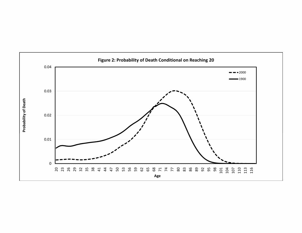
above. Specifically, we focus on the change in the uncertainty regarding mortality. This point can be seen
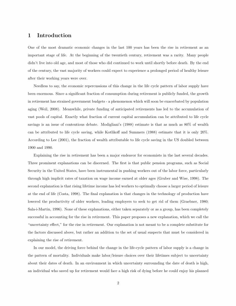
most clearly by looking at Figure 2. The figure shows the probability of dying at different ages, conditional
on having reached age 20, using the cross-sectional male life tables for 1900 and 2000. The fact that the
mean age of death goes up (from 61.2 to 73.9) is hardly surprising. What is more interesting is that the
standard deviation of the age of death falls, from 18.1 to 14.2. And of course the coefficient of variation in
the age of death (the standard deviation divided by the mean) falls by even more, from 0.30 to 0.19. By
2050, the mean age of death is expected to rise further, to 76.5, while the standard deviation will also rise,
to 15.4. The coefficient of variation will remain almost exactly constant.
How should declining mortality affect the retirement age? Two different forces are at work. First, and
most intuitively, longer life would be expected to increase the number of years during which an individual
plans to work, simply because longer life means that there will be more years of consumption which need to
be paid for. We call this channel the “horizon effect” of increased life expectancy. But a second effect arises
from the fact that increases in life expectancy may reduce the uncertainty surrounding whether a person will
live into old age. Where mortality is high, individuals are unlikely to live into old age, and so any savings
for a planned retirement would likely be wasted. The optimal program in such circumstances would be to
plan continue working in old age, should such an eventuality arise. In this case, a reduction in mortality,
by making survival into old age more likely, can reduce the planned age of retirement. We call this second
channel the “uncertainty effect.”
Whether the uncertainty effect or the horizon effect of increased life expectancy is more important depends
on the manner in which life expectancy increases, as well as on the nature of the individual’s optimization
problem. We set up the general problem in Section 3.1, and also show that if life expectancy rises in the
context of certainty (or when there is a full set of annuities available), retirement age rises as well. We then
consider three different forms of the survival function, in which we can model increases in life expenditure.
7
We begin in Section 3.2 by using an exponential model of survival, which is unrealistic but mathematically
simple. In Section 3.2 we apply a more realistic two-parameter model of survival introduced by Boucekkine,
de la Croix, and Licandro (2002). Finally, in Section 3.3 we use actual data on changes in adult survival in
the United States.
3.1 Setup of the Problem
Consider an individual who receives utility from both consumption and leisure. We assume that there are
only two possible levels of labor supply: a person may either be fully employed or retired. We also assume
that once a person retires, he may not re-enter the labor force.11 Let γ represent the increment to utility
from leisure due to retirement (that is, the difference between utility from leisure before retirement and
after). For convenience, utility from leisure and consumption are taken to be separable. The instantaneous
utility function is12
U = ln(c) if working (1)
= ln(c) + γ if retired.
An important feature of this utility function is that marginal utility of retirement leisure does not decline
with the length of retirement – that is, there are no decreasing returns to retirement.
The assumption that utility from consumption is given by the log function is made so that changes in
wages will not, by themselves, affect the optimal age of retirement. In general, changes in wages (holding
interest rates and mortality constant) will have both income and substitution effects on the demand for end-
of-life leisure. With log utility these just balance each other, and so the derivative of the optimal retirement
age with respect to the wage is zero. If utility is more curved than the log function, then the income effect
will dominate, and increases in wages will lead to a reduction in the optimal retirement age. We explore this
effect further in Section 5.
Future utility is discounted at rate θ. Thus we can write lifetime utility as,
11The question of why retirement usually takes the form of a sudden and complete withdrawal from the labor force is adifficult one, and we do not address it here.
12To be clear, we are starting with more general utility function of the form U = ln(c) + f(n), where f(n), the subutilityfrom leisure, has the standard properties including a positive first derivative and negative second derivative. Our assumptionis that n can take only two values, nw for people who are working and nr for people who are retired. Thus γ = f(nr)− f(nw).
8
U =
∫ T
0
e−θx[ln(c(x))]dx+
∫ T
R
e−θx[γ]dx, (2)
where R is the age or retirement, T is the age of death, and R ≤ T. We take age zero to be the beginning
of adulthood. We abstract from fertility and child-rearing costs.
In the case where the date of death is uncertain, expected lifetime utility is given by
E(U) =
∫ ∞
0
e−θxP (x)[ln(c(x))]dx+
∫ ∞
R
e−θxP (x)[γ]dx, (3)
where P (x) is the probability of being alive at age x. Note that in this case, R is the planned age of
retirement, but an individual who dies before age R will not experience any retirement at all. Since the only
uncertainty that we admit to the model is about the date of death, and since this uncertainty is not resolved
until it is too late to do anything about it, individuals will form time-consistent plans for consumption and
retirement at the beginning of their lives.
Individuals who are working receive a wage of w. The real interest rate is r. We impose the condition
that assets must be non-negative at all times. Although the exact justification for such a debt constraint is
not relevant for our purposes, a reasonable assumption is that it results from capital market imperfections
that prevent individuals from borrowing against their future labor income. Carroll (2001, figure 2) shows
that non-collateralized debt is indeed very small relative to lifetime income. Solving our problem under the
assumption that there is a small but non-zero limit on debt yields nearly identical results.
3.1.1 Optimal Retirement with No Uncertainty
We begin by considering the case where the date of death, T, is known with certainty. The individual’s
lifetime budget constraint is
∫ R
0
e−rx[w]dx =
∫ T
0
e−rx[c(x)]dx. (4)
The individual will maximize his utility subject to his budget constraint by choosing a path of life-
time consumption, c(x), and an endogenous retirement age, R. The first order condition with respect to
consumption implies,
c(x) = [r − θ]c(x) (5)
9
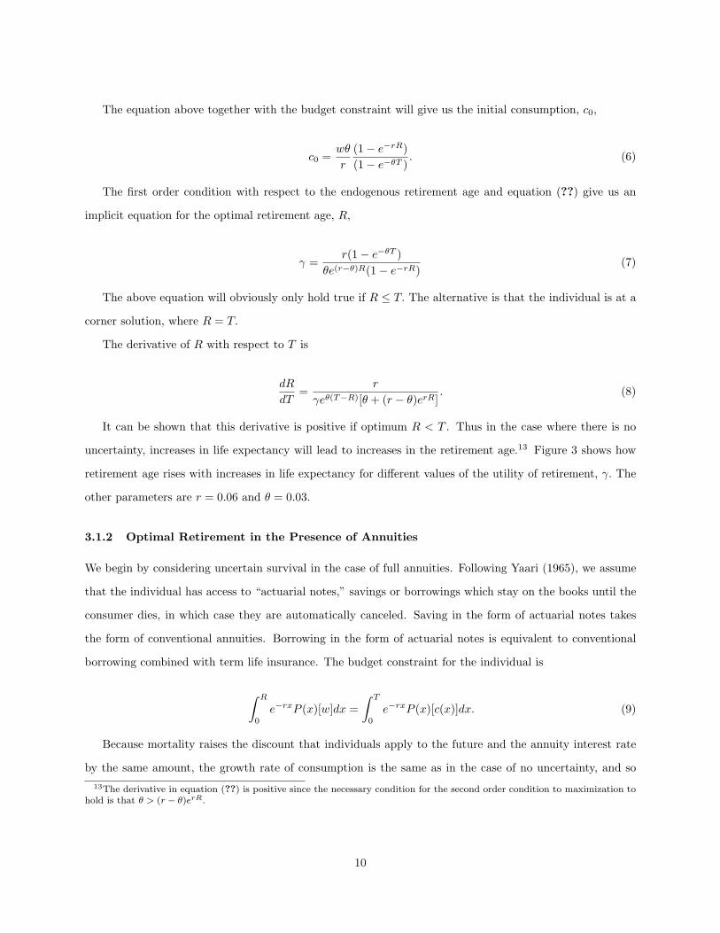
The equation above together with the budget constraint will give us the initial consumption, c0,
c0 =wθ
r
(1− e−rR)
(1− e−θT ). (6)
The first order condition with respect to the endogenous retirement age and equation (??) give us an
implicit equation for the optimal retirement age, R,
γ =r(1− e−θT )
θe(r−θ)R(1− e−rR)(7)
The above equation will obviously only hold true if R ≤ T. The alternative is that the individual is at a
corner solution, where R = T.
The derivative of R with respect to T is
dR
dT=
r
γeθ(T−R)[θ + (r − θ)erR]. (8)
It can be shown that this derivative is positive if optimum R < T . Thus in the case where there is no
uncertainty, increases in life expectancy will lead to increases in the retirement age.13 Figure 3 shows how
retirement age rises with increases in life expectancy for different values of the utility of retirement, γ. The
other parameters are r = 0.06 and θ = 0.03.
3.1.2 Optimal Retirement in the Presence of Annuities
We begin by considering uncertain survival in the case of full annuities. Following Yaari (1965), we assume
that the individual has access to “actuarial notes,” savings or borrowings which stay on the books until the
consumer dies, in which case they are automatically canceled. Saving in the form of actuarial notes takes
the form of conventional annuities. Borrowing in the form of actuarial notes is equivalent to conventional
borrowing combined with term life insurance. The budget constraint for the individual is
∫ R
0
e−rxP (x)[w]dx =
∫ T
0
e−rxP (x)[c(x)]dx. (9)
Because mortality raises the discount that individuals apply to the future and the annuity interest rate
by the same amount, the growth rate of consumption is the same as in the case of no uncertainty, and so
13The derivative in equation (??) is positive since the necessary condition for the second order condition to maximization tohold is that θ > (r − θ)erR.
10
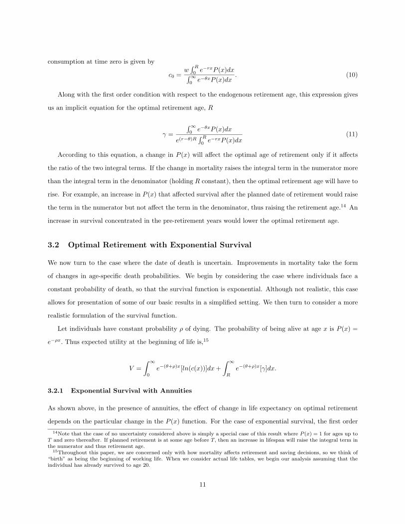
consumption at time zero is given by
c0 =w∫ R
0e−rxP (x)dx∫∞
0e−θxP (x)dx
. (10)
Along with the first order condition with respect to the endogenous retirement age, this expression gives
us an implicit equation for the optimal retirement age, R
γ =
∫∞0
e−θxP (x)dx
e(r−θ)R∫ R
0e−rxP (x)dx
(11)
According to this equation, a change in P (x) will affect the optimal age of retirement only if it affects
the ratio of the two integral terms. If the change in mortality raises the integral term in the numerator more
than the integral term in the denominator (holding R constant), then the optimal retirement age will have to
rise. For example, an increase in P (x) that affected survival after the planned date of retirement would raise
the term in the numerator but not affect the term in the denominator, thus raising the retirement age.14 An
increase in survival concentrated in the pre-retirement years would lower the optimal retirement age.
3.2 Optimal Retirement with Exponential Survival
We now turn to the case where the date of death is uncertain. Improvements in mortality take the form
of changes in age-specific death probabilities. We begin by considering the case where individuals face a
constant probability of death, so that the survival function is exponential. Although not realistic, this case
allows for presentation of some of our basic results in a simplified setting. We then turn to consider a more
realistic formulation of the survival function.
Let individuals have constant probability ρ of dying. The probability of being alive at age x is P (x) =
e−ρx. Thus expected utility at the beginning of life is,15
V =
∫ ∞
0
e−(θ+ρ)x[ln(c(x))]dx+
∫ ∞
R
e−(θ+ρ)x[γ]dx.
3.2.1 Exponential Survival with Annuities
As shown above, in the presence of annuities, the effect of change in life expectancy on optimal retirement
depends on the particular change in the P (x) function. For the case of exponential survival, the first order
14Note that the case of no uncertainty considered above is simply a special case of this result where P (x) = 1 for ages up toT and zero thereafter. If planned retirement is at some age before T, then an increase in lifespan will raise the integral term inthe numerator and thus retirement age.
15Throughout this paper, we are concerned only with how mortality affects retirement and saving decisions, so we think of“birth” as being the beginning of working life. When we consider actual life tables, we begin our analysis assuming that theindividual has already survived to age 20.
11
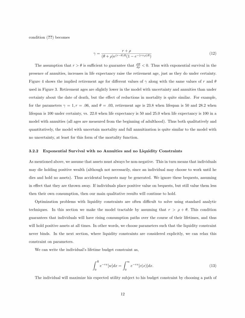
condition (??) becomes
γ =r + ρ
(θ + ρ)e(r−θ)R(1− e−(r+ρ)R)(12)
The assumption that r > θ is sufficient to guarantee that dRdρ < 0. Thus with exponential survival in the
presence of annuities, increases in life expectancy raise the retirement age, just as they do under certainty.
Figure 4 shows the implied retirement age for different values of γ along with the same values of r and θ
used in Figure 3. Retirement ages are slightly lower in the model with uncertainty and annuities than under
certainty about the date of death, but the effect of reductions in mortality is quite similar. For example,
for the parameters γ = 1, r = .06, and θ = .03, retirement age is 23.8 when lifespan is 50 and 28.2 when
lifespan is 100 under certainty, vs. 22.0 when life expectancy is 50 and 25.0 when life expectancy is 100 in a
model with annuities (all ages are measured from the beginning of adulthood). Thus both qualitatively and
quantitatively, the model with uncertain mortality and full annuitization is quite similar to the model with
no uncertainty, at least for this form of the mortality function.
3.2.2 Exponential Survival with no Annuities and no Liquidity Constraints
As mentioned above, we assume that assets must always be non-negative. This in turn means that individuals
may die holding positive wealth (although not necessarily, since an individual may choose to work until he
dies and hold no assets). Thus accidental bequests may be generated. We ignore these bequests, assuming
in effect that they are thrown away. If individuals place positive value on bequests, but still value them less
then their own consumption, then our main qualitative results will continue to hold.
Optimization problems with liquidity constraints are often difficult to solve using standard analytic
techniques. In this section we make the model tractable by assuming that r > ρ + θ. This condition
guarantees that individuals will have rising consumption paths over the course of their lifetimes, and thus
will hold positive assets at all times. In other words, we choose parameters such that the liquidity constraint
never binds. In the next section, where liquidity constraints are considered explicitly, we can relax this
constraint on parameters.
We can write the individual’s lifetime budget constraint as,
∫ R
0
e−rx[w]dx =
∫ ∞
0
e−rx[c(x)]dx. (13)
The individual will maximize his expected utility subject to his budget constraint by choosing a path of
12
lifetime consumption, c(x), and an endogenous retirement age, R. The first order condition with respect to
consumption implies,
c(x) = [r − θ − ρ]c(x) (14)
The equation above together with the budget constraint will give us the initial consumption, c0,
c0 =w(θ + ρ)
r
[1− e−rR
]. (15)
We can now re-write the individual’s expected lifetime utility as a function of planned retirement age,
R. Ignoring terms that do not contain R,
V (R) =1
θ + ρln(1− e−rR) + γ
e−(θ+ρ)R
θ + ρ(16)
Figure 5 shows how the V(R) function changes with life expectancy (the other parameters are as above).
For high values of ρ, that is, when life expectancy is low, the V(R) function is upward sloping. In this case,
the optimum is a corner solution of R = ∞; in other words, the individual plans never to retire. For low
values of ρ, in other words when life expectancy is high, there is a single interior solution.16
Figure 6 show the relationship between retirement and life expectancy (which is just 1/ρ) for the same
parameters used in Figures 3 and 4. Notice that R is the planned age of retirement, but that many people
will not live long enough to reach it. Thus there is no inconsistency in having the retirement age be greater
than life expectancy. Figure 6 shows the key result: as life expectancy rises, the planned age of retirement
falls.
Figures 3, 4, and 6 allow for an explicit analysis of the role of uncertainty in affecting retirement.
Comparing either Figure 3 or Figure 4, on the one hand, to Figure 6, on the other, shows the effect of
uncertainty on optimal retirement age. (The fact that Figures 3 and 4 are so similar shows that annuities
16This can be shown formally, as follows. From ??, the first order condition for optimal retirement age is
r
γ(θ + ρ)= e(r−θ−ρ)R
[(1− e−rR)
].
The effect of mortality on the optimal retirement age is given by the equation.
dR
dρ= −
−Re(r−ρ−θ)R +Re−(ρ+θ)R + r/(γθ + ρ)2
(r − ρ− θ)e(r−ρ−θ)R + (ρ+ θ)e−(ρ+θ)R.
It can be shown that this derivative is positive for large values of R. Thus, the initial effect of reductions in mortality (startingfrom a high level of ρ) will be to reduce the age of retirement. However, once retirement age has fallen, it is possible thatfurther improvements in mortality can raise the age of retirement. Specifically, retirement falls with life expectancy as long asR > 1
θ+ρ
13
and insurance can eliminate most of the effect of uncertainty on retirement age.) The rise in retirement
age with life expectancy in either Figure 3 or Figure 4 is what we call the “horizon effect.” The fact that
optimal retirement falls with life expectancy in Figure 6 shows that the decline in retirement age due to
falling uncertainty more than compensates for the rise due to longer horizons.
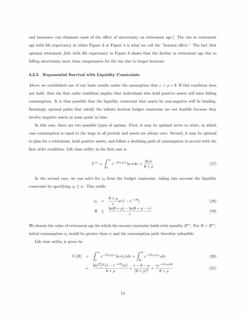
3.2.3 Exponential Survival with Liquidity Constraints
Above we established one of our basic results under the assumption that r > ρ + θ. If this condition does
not hold, then the first order condition implies that individuals who hold positive assets will have falling
consumption. It is thus possible that the liquidity constraint that assets be non-negative will be binding.
Seemingly optimal paths that satisfy the infinite horizon budget constraint are not feasible because they
involve negative assets at some point in time.
In this case, there are two possible types of optima. First, it may be optimal never to retire, in which
case consumption is equal to the wage in all periods and assets are always zero. Second, it may be optimal
to plan for a retirement, hold positive assets, and follow a declining path of consumption in accord with the
first order condition. Life time utility in the first case is
U∗∗ =
∫ ∞
0
e−(θ+ρ)x lnwdx =lnw
θ + ρ(17)
In the second case, we can solve for c0 from the budget constraint, taking into account the liquidity
constraint by specifying c0 ≤ w. This yields
c0 =θ + ρ
rw(1− e−rR) (18)
R ≤ ln(θ + ρ)− ln(θ + ρ− r)
r(19)
We denote the value of retirement age for which the second constraint holds with equality R∗∗. For R > R∗∗,
initial consumption c0 would be greater than w and the consumption path therefore infeasible.
Life time utility is given by
V (R) =
∫ ∞
0
e−(θ+ρ)x ln c(x)dx+
∫ ∞
R
e−(θ+ρ)xγdx (20)
=ln( θ+ρ
r (1− e−rR)w)
θ + ρ+
r − θ − ρ
(θ + ρ)2+
γe−(θ+ρ)R
θ + ρ(21)
14
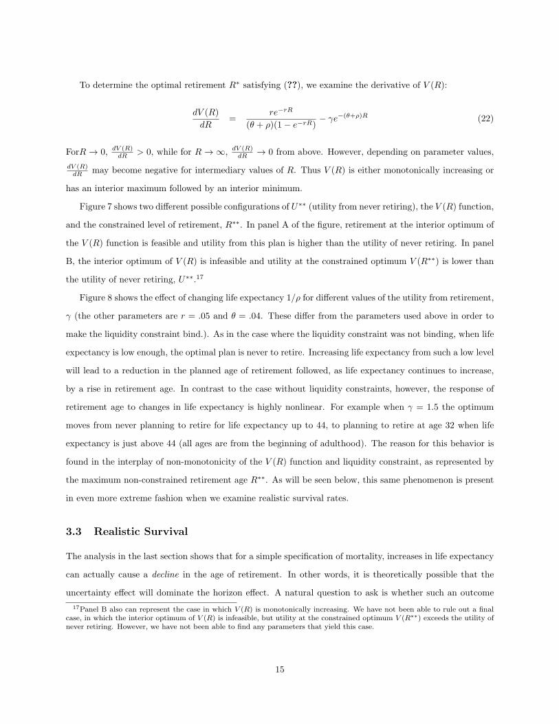
To determine the optimal retirement R∗ satisfying (??), we examine the derivative of V (R):
dV (R)
dR=
re−rR
(θ + ρ)(1− e−rR)− γe−(θ+ρ)R (22)
ForR → 0, dV (R)dR > 0, while for R → ∞, dV (R)
dR → 0 from above. However, depending on parameter values,
dV (R)dR may become negative for intermediary values of R. Thus V (R) is either monotonically increasing or
has an interior maximum followed by an interior minimum.
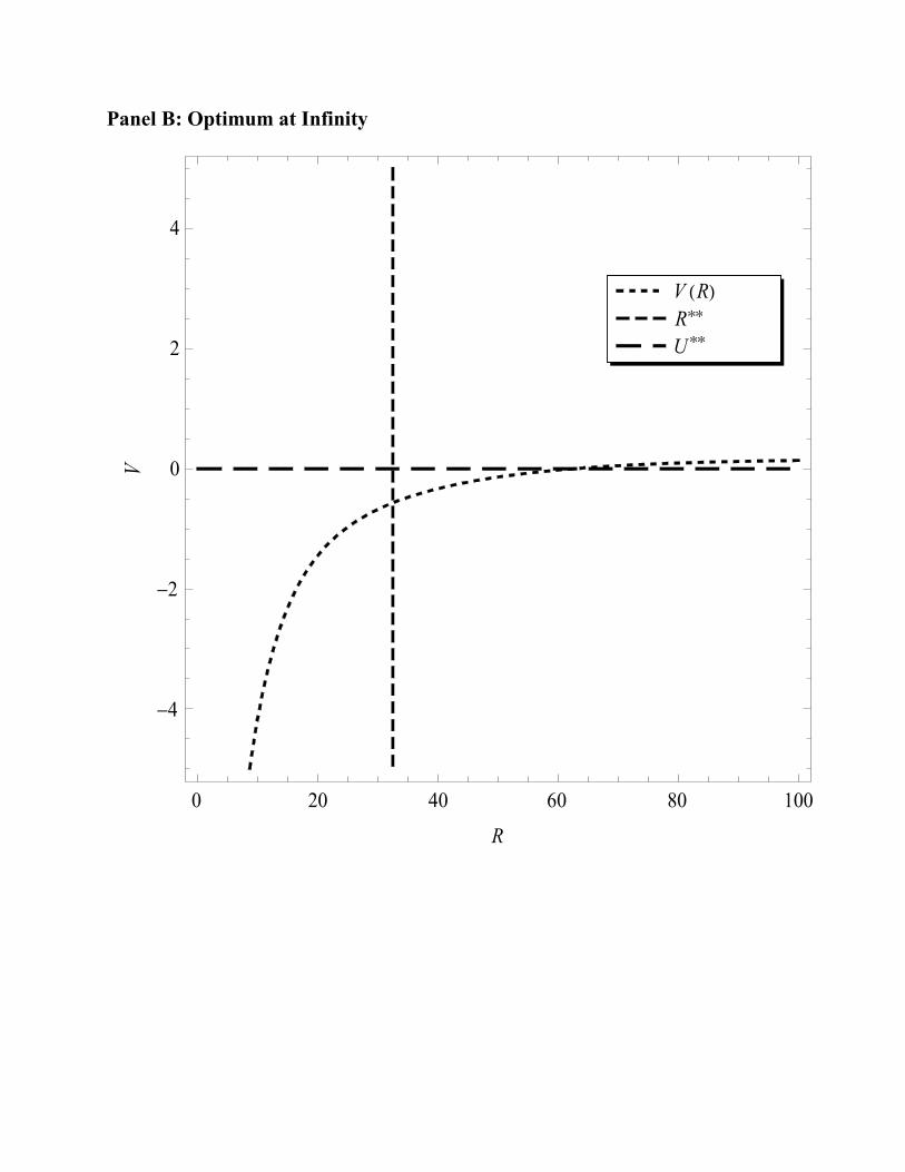
Figure 7 shows two different possible configurations of U∗∗ (utility from never retiring), the V (R) function,
and the constrained level of retirement, R∗∗. In panel A of the figure, retirement at the interior optimum of
the V (R) function is feasible and utility from this plan is higher than the utility of never retiring. In panel
B, the interior optimum of V (R) is infeasible and utility at the constrained optimum V (R∗∗) is lower than
the utility of never retiring, U∗∗.17
Figure 8 shows the effect of changing life expectancy 1/ρ for different values of the utility from retirement,
γ (the other parameters are r = .05 and θ = .04. These differ from the parameters used above in order to
make the liquidity constraint bind.). As in the case where the liquidity constraint was not binding, when life
expectancy is low enough, the optimal plan is never to retire. Increasing life expectancy from such a low level
will lead to a reduction in the planned age of retirement followed, as life expectancy continues to increase,
by a rise in retirement age. In contrast to the case without liquidity constraints, however, the response of
retirement age to changes in life expectancy is highly nonlinear. For example when γ = 1.5 the optimum
moves from never planning to retire for life expectancy up to 44, to planning to retire at age 32 when life
expectancy is just above 44 (all ages are from the beginning of adulthood). The reason for this behavior is
found in the interplay of non-monotonicity of the V (R) function and liquidity constraint, as represented by
the maximum non-constrained retirement age R∗∗. As will be seen below, this same phenomenon is present
in even more extreme fashion when we examine realistic survival rates.
3.3 Realistic Survival
The analysis in the last section shows that for a simple specification of mortality, increases in life expectancy
can actually cause a decline in the age of retirement. In other words, it is theoretically possible that the
uncertainty effect will dominate the horizon effect. A natural question to ask is whether such an outcome
17Panel B also can represent the case in which V (R) is monotonically increasing. We have not been able to rule out a finalcase, in which the interior optimum of V (R) is infeasible, but utility at the constrained optimum V (R∗∗) exceeds the utility ofnever retiring. However, we have not been able to find any parameters that yield this case.
15
is consistent with actual changes in mortality that have been experienced historically. We proceed in two
stages. First, we consider a tractable but realistic model of survival in which we can derive results analytically.
Following this, we look at actual data on survival in the United States and calculate optimal retirement ages
numerically.
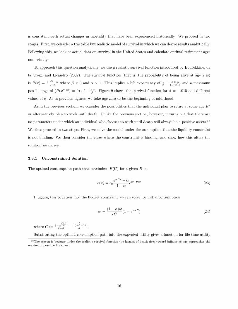
To approach this question analytically, we use a realistic survival function introduced by Boucekkine, de
la Croix, and Licandro (2002). The survival function (that is, the probability of being alive at age x is)
is P (x) = e−βx−α1−α where β < 0 and α > 1. This implies a life expectancy of 1
β + α lnα(1−α)β and a maximum
possible age of (P (xmax) = 0) of − lnαβ . Figure 9 shows the survival function for β = −.015 and different
values of α. As in previous figures, we take age zero to be the beginning of adulthood.
As in the previous section, we consider the possibilities that the individual plan to retire at some age R∗
or alternatively plan to work until death. Unlike the previous section, however, it turns out that there are
no parameters under which an individual who chooses to work until death will always hold positive assets.18
We thus proceed in two steps. First, we solve the model under the assumption that the liquidity constraint
is not binding. We then consider the cases where the constraint is binding, and show how this alters the
solution we derive.
3.3.1 Unconstrained Solution
The optimal consumption path that maximizes E(U) for a given R is
c(x) = c0e−βx − α
1− αe(r−θ)x (23)
Plugging this equation into the budget constraint we can solve for initial consumption
c0 =(1− α)w
rC(1− e−rR) (24)
where C := 1−αθ+ββ
θ+β + α(αθβ −1)θ .
Substituting the optimal consumption path into the expected utility gives a function for life time utility
18The reason is because under the realistic survival function the hazard of death rises toward infinity as age approaches themaximum possible life span.
16
in terms of R (leaving out terms without R):
V (R) = ln(1− e−rR)
∫ T
0
e−βx − α
1− αe−θxdx+ γ
∫ T
R
e−βx − α
1− αe−θxdx (25)
=ln(1− e−rR)
1− αC +
γ
1− α(e−(β+θ)R − α
θ+ββ
θ + β+
α(αθβ − e−θR)
θ) (26)
Figure 10 plots V (R) for different values of α (in each case, the function is plotted only up to R = xmax.
The other parameters are set as above: β = −.015, r = .06, θ = .03, γ = 1. For α ≥ 2.22 (life expectancy
= 30 years, xmax = 50 years), V (R) has a local maximum followed by a local minimum, after which the
function increases monotonically. Label the local maximum R∗. If V (R∗) ≥ U∗∗ it is optimal to retire at
age R∗, otherwise it is optimal to never retire. Graphically, one can see that never retiring is optimal for
values of α below a certain threshold (α ≈ 2.45, implying life expectancy ≈ 35 years, xmax ≈ 61 years).
3.3.2 Constrained Solution
As mentioned above, under realistic survival it is always the case that an individual who chooses to work
until death will hold zero assets at some age – in other words, the liquidity constraint is always binding at
some point in time. In particular, if one looks at the paths of assets implied by the unconstrained V (R)
function in the previous section, in the case where an individual never retires, assets are negative in the
period immediately before the maximum possible age. We thus define V (R) as the utility resulting from
retirement at age R taking into account the liquidity constraint. V (R) will be equal to V (R) up to some
critical retirement age R∗∗, and then will lie below it.
We were not able to derive an analytic expression for V (R). Instead, we solve for the function by brute
force. For each possible retirement age, we first check whether the path of assets implied by the unconstrained
solution is ever negative. If this is not the case, then ˜V (R) = V (R). If it is the case, we solve for utility along
a constrained path which involves holding positive assets and working up until some age x∗, then setting
income equal to consumption between ages x∗ and x∗∗, then building up assets again between age x∗∗ and
retirement.19. Figure 11 shows an example of the how the V (R) and V (R) functions compare for a particular
set of parameters (α = 2.45 and all other parameters as above). The case is chosen in particular to show
how it is possible for V (xmax)) > V (R∗) but V (xmax) < V (R∗). In other words, using the unconstrained
V (R) function, never retiring is optimal, while recognizing the liquidity constraint, retiring at an interior
optimum R∗ is optimal.
19The Matlab code is available on request
17

Despite this example, the general properties of the V (R) are quite similar to those of the V (R) function
(and the set of parameters for which optimal retirement implied by the two differ is quite small). Specifically,
there is an interior optimum and a corner solution of R = xmax. Small changes in the parameters, such as
the shape of the survival function or the utility from retirement, can lead to a shift in the utility maximizing
age of retirement from a corner solution to an interior optimum. Figure 12 shows how the optimal age of
retirement changes with life expectancy (as the parameter α varies) for different values of the utility from
retirement, γ.
The important implication of figure 12 is that because of the structure of the V (R) function, small changes
in the parameters will lead to large changes in expected retirement age. The pattern of the V(R) function
in which the two possible global optima are an interior optimum and a corner solution results from the
dichotomy between the two strategies for optimal consumption mentioned above: to plan for a retirement,
with the risk that one might die early and thus have wasted all of the money saved up; or to plan to pay
for consumption in the event that one lives into old age by working. There is no way within the model to
“convexify” between these two strategies.
Taken literally, this result would imply that there should be a sudden shift in behavior from never retiring
to planning for a large retirement. Obviously this is not what is observed in the data, where the growth of
retirement has been rapid (in historical terms) but hardly instantaneous. We do not think of this as a major
failing of the model. In the real world, heterogeneity, institutions, learning, and a host of other factors would
tend to cause retirement ages to adjust slowly, rather than jumping all at once, in response to a change in
mortality.
3.4 Optimal Retirement with Actual Survival Rates
Although the realistic survival function shown in Figure 9 are obviously a great improvement on the ex-
ponential model of survival considered in Section 3.2, it still is not a precise match to the actual survival
schedules show in Figure 1. Thus as a final exercise we examine the effect of actually observed mortality
changes.
We use a discrete time version of our model to calculate optimal retirement ages for actual mortality
data. Our procedure for finding the optimal retirement age is straightforward. We loop through possible
retirement ages, and calculate optimal consumption and asset paths for each one subject to the constraint
that assets are never negative.20 We then calculate expected utility associated with each possible retirement
20Let Pt be the probability that an individual will be alive in period t, and let At be assets at the beginning of the period.
18
age.
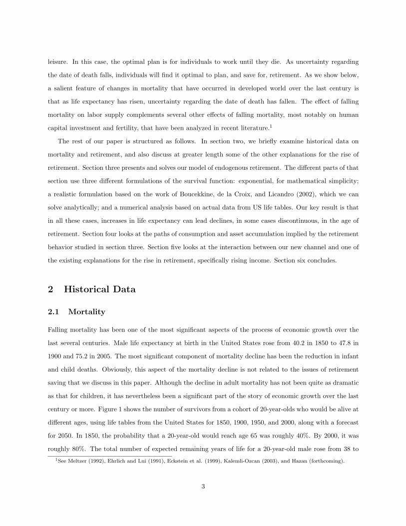
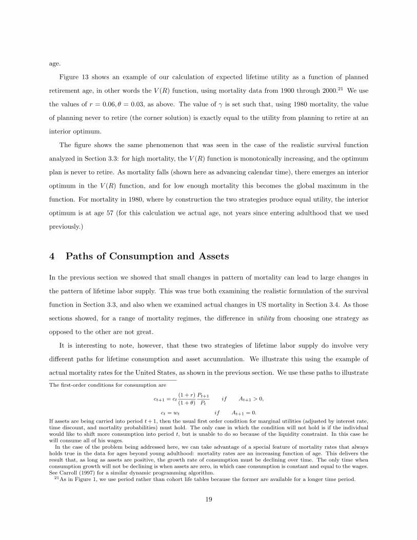
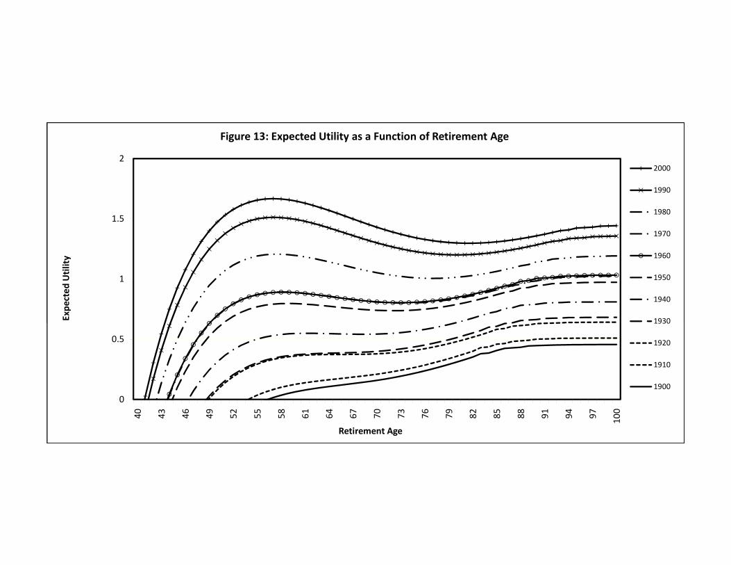
Figure 13 shows an example of our calculation of expected lifetime utility as a function of planned
retirement age, in other words the V (R) function, using mortality data from 1900 through 2000.21 We use
the values of r = 0.06, θ = 0.03, as above. The value of γ is set such that, using 1980 mortality, the value
of planning never to retire (the corner solution) is exactly equal to the utility from planning to retire at an
interior optimum.
The figure shows the same phenomenon that was seen in the case of the realistic survival function
analyzed in Section 3.3: for high mortality, the V (R) function is monotonically increasing, and the optimum
plan is never to retire. As mortality falls (shown here as advancing calendar time), there emerges an interior
optimum in the V (R) function, and for low enough mortality this becomes the global maximum in the
function. For mortality in 1980, where by construction the two strategies produce equal utility, the interior
optimum is at age 57 (for this calculation we actual age, not years since entering adulthood that we used
previously.)
4 Paths of Consumption and Assets
In the previous section we showed that small changes in pattern of mortality can lead to large changes in
the pattern of lifetime labor supply. This was true both examining the realistic formulation of the survival
function in Section 3.3, and also when we examined actual changes in US mortality in Section 3.4. As those
sections showed, for a range of mortality regimes, the difference in utility from choosing one strategy as
opposed to the other are not great.
It is interesting to note, however, that these two strategies of lifetime labor supply do involve very
different paths for lifetime consumption and asset accumulation. We illustrate this using the example of
actual mortality rates for the United States, as shown in the previous section. We use these paths to illustrate
The first-order conditions for consumption are
ct+1 = ct(1 + r)
(1 + θ)
Pt+1
Ptif At+1 > 0,
ct = wt if At+1 = 0.
If assets are being carried into period t+1, then the usual first order condition for marginal utilities (adjusted by interest rate,time discount, and mortality probabilities) must hold. The only case in which the condition will not hold is if the individualwould like to shift more consumption into period t, but is unable to do so because of the liquidity constraint. In this case hewill consume all of his wages.
In the case of the problem being addressed here, we can take advantage of a special feature of mortality rates that alwaysholds true in the data for ages beyond young adulthood: mortality rates are an increasing function of age. This delivers theresult that, as long as assets are positive, the growth rate of consumption must be declining over time. The only time whenconsumption growth will not be declining is when assets are zero, in which case consumption is constant and equal to the wages.See Carroll (1997) for a similar dynamic programming algorithm.
21As in Figure 1, we use period rather than cohort life tables because the former are available for a longer time period.
19
the qualitative change in the lifetime pattern of asset holdings that takes place when retirement behavior
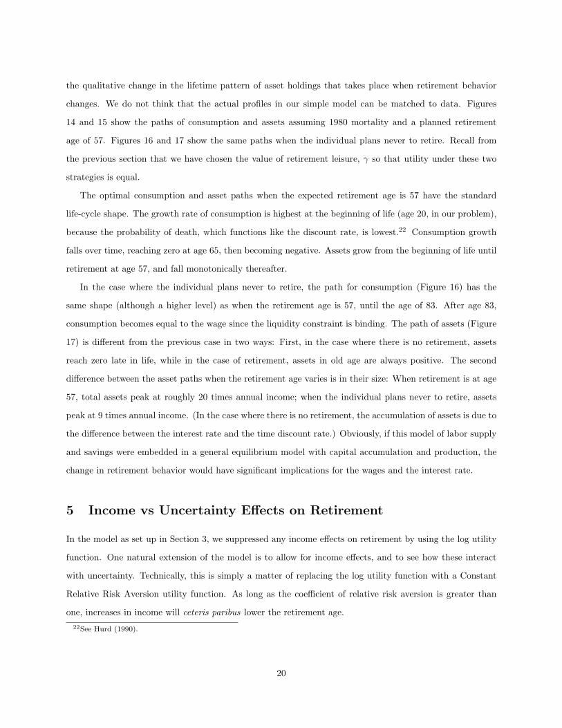
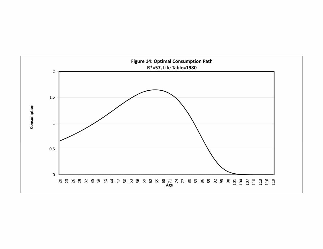
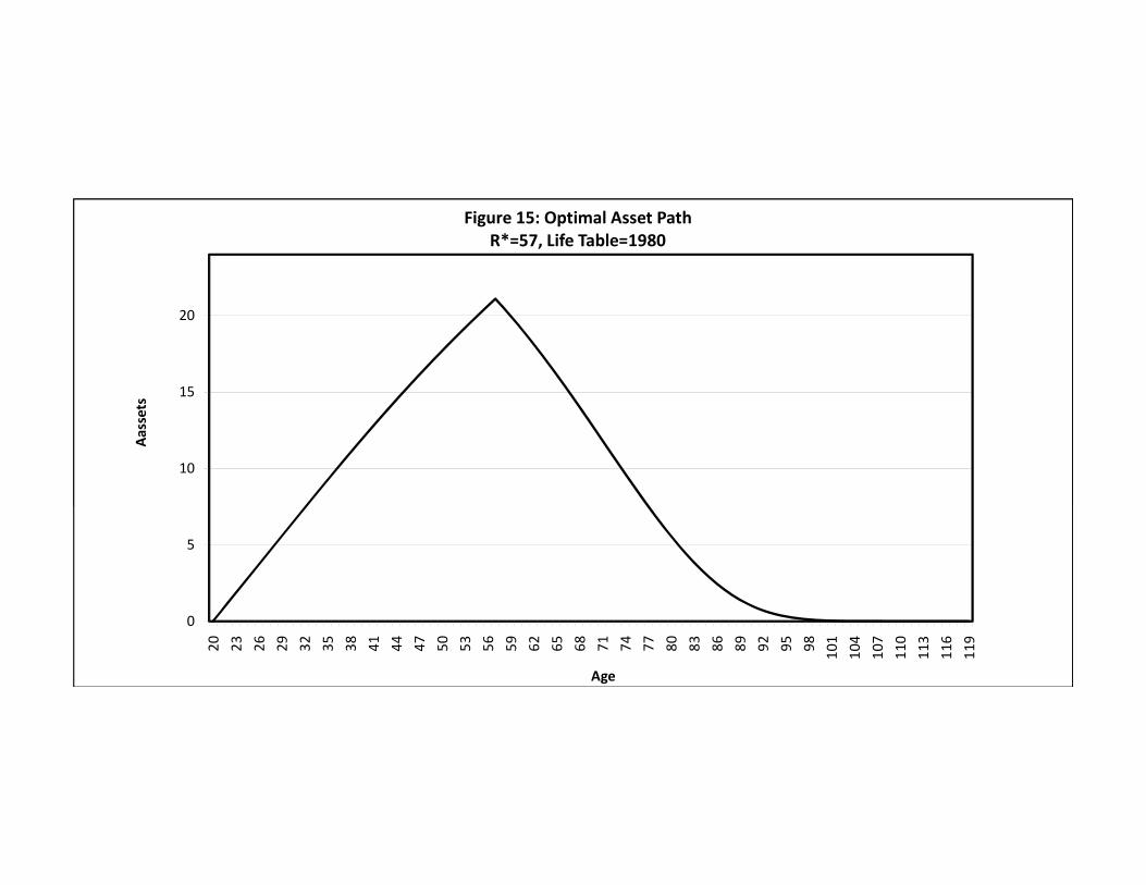
changes. We do not think that the actual profiles in our simple model can be matched to data. Figures
14 and 15 show the paths of consumption and assets assuming 1980 mortality and a planned retirement
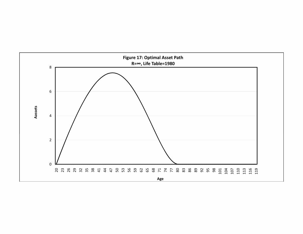
age of 57. Figures 16 and 17 show the same paths when the individual plans never to retire. Recall from
the previous section that we have chosen the value of retirement leisure, γ so that utility under these two
strategies is equal.
The optimal consumption and asset paths when the expected retirement age is 57 have the standard
life-cycle shape. The growth rate of consumption is highest at the beginning of life (age 20, in our problem),
because the probability of death, which functions like the discount rate, is lowest.22 Consumption growth
falls over time, reaching zero at age 65, then becoming negative. Assets grow from the beginning of life until
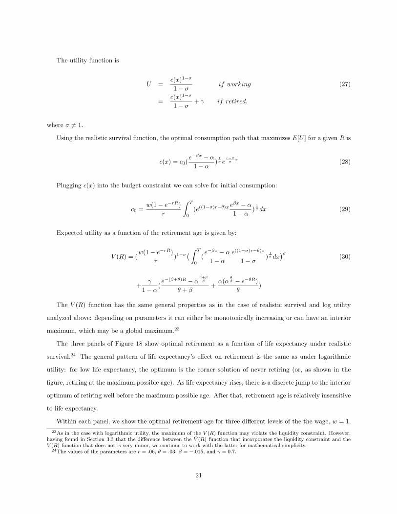
retirement at age 57, and fall monotonically thereafter.
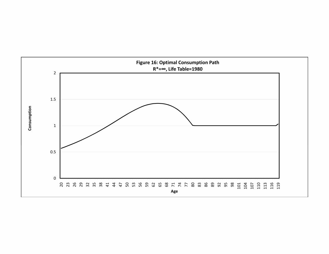
In the case where the individual plans never to retire, the path for consumption (Figure 16) has the
same shape (although a higher level) as when the retirement age is 57, until the age of 83. After age 83,
consumption becomes equal to the wage since the liquidity constraint is binding. The path of assets (Figure
17) is different from the previous case in two ways: First, in the case where there is no retirement, assets
reach zero late in life, while in the case of retirement, assets in old age are always positive. The second
difference between the asset paths when the retirement age varies is in their size: When retirement is at age
57, total assets peak at roughly 20 times annual income; when the individual plans never to retire, assets
peak at 9 times annual income. (In the case where there is no retirement, the accumulation of assets is due to
the difference between the interest rate and the time discount rate.) Obviously, if this model of labor supply
and savings were embedded in a general equilibrium model with capital accumulation and production, the
change in retirement behavior would have significant implications for the wages and the interest rate.
5 Income vs Uncertainty Effects on Retirement
In the model as set up in Section 3, we suppressed any income effects on retirement by using the log utility
function. One natural extension of the model is to allow for income effects, and to see how these interact
with uncertainty. Technically, this is simply a matter of replacing the log utility function with a Constant
Relative Risk Aversion utility function. As long as the coefficient of relative risk aversion is greater than
one, increases in income will ceteris paribus lower the retirement age.
22See Hurd (1990).
20
The utility function is
U =c(x)1−σ
1− σif working (27)
=c(x)1−σ
1− σ+ γ if retired.
where σ = 1.
Using the realistic survival function, the optimal consumption path that maximizes E[U ] for a given R is
c(x) = c0(e−βx − α
1− α)
1σ e
r−θσ x (28)
Plugging c(x) into the budget constraint we can solve for initial consumption:
c0 =w(1− e−rR)
r
∫ T
0
(e((1−σ)r−θ)x eβx − α
1− α)
1σ dx (29)
Expected utility as a function of the retirement age is given by:
V (R) = (w(1− e−rR)
r)1−σ
( ∫ T
0
(e−βx − α
1− α
e((1−σ)r−θ)x
1− σ)
1σ dx
)σ(30)
+γ
1− α(e−(β+θ)R − α
θ+ββ
θ + β+
α(αθβ − e−θR)
θ)
The V (R) function has the same general properties as in the case of realistic survival and log utility
analyzed above: depending on parameters it can either be monotonically increasing or can have an interior
maximum, which may be a global maximum.23
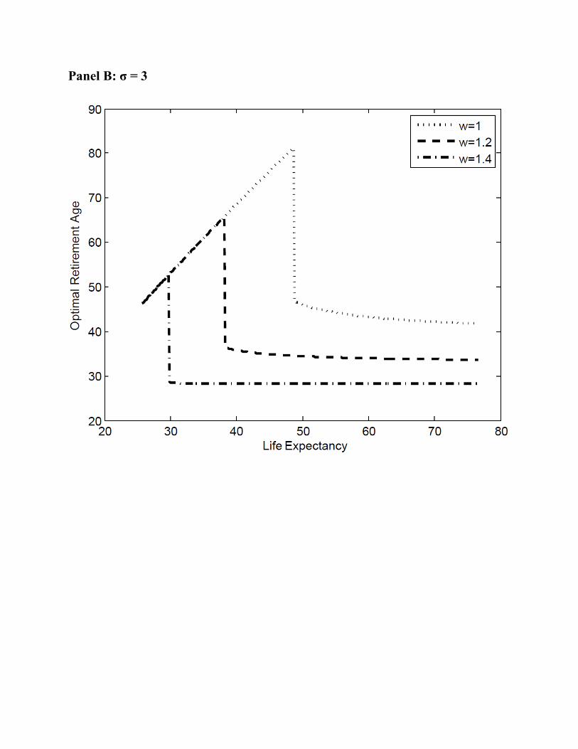
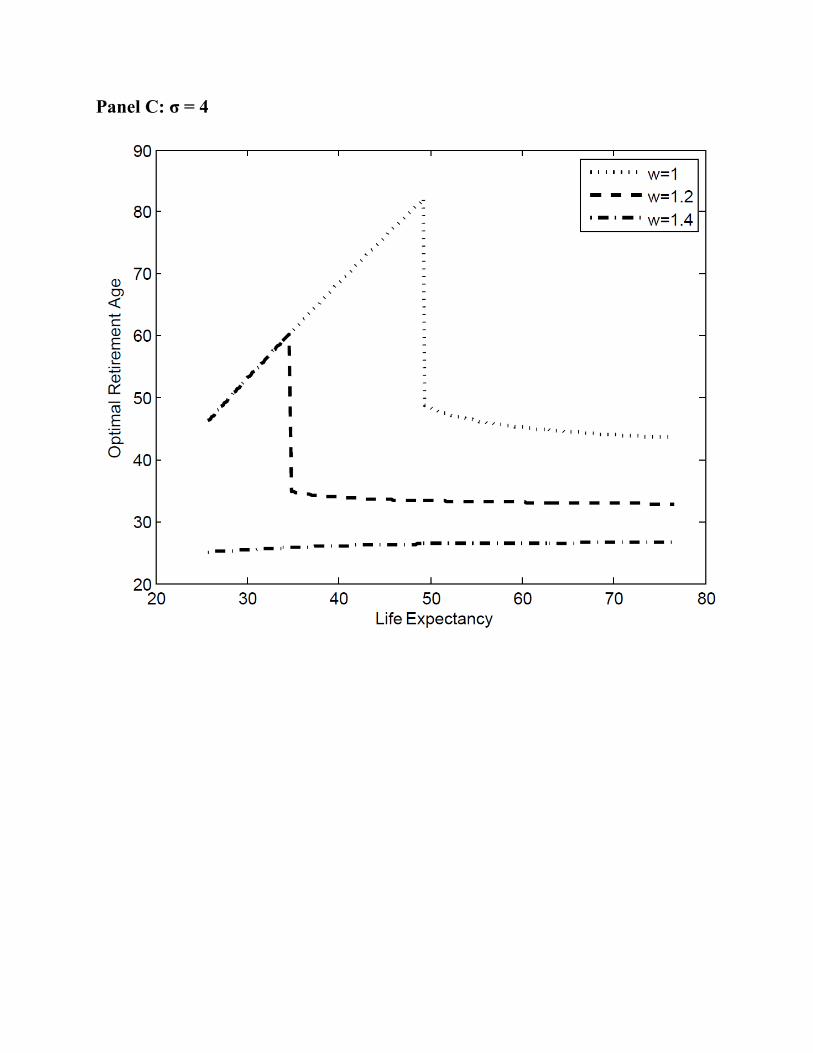
The three panels of Figure 18 show optimal retirement as a function of life expectancy under realistic
survival.24 The general pattern of life expectancy’s effect on retirement is the same as under logarithmic
utility: for low life expectancy, the optimum is the corner solution of never retiring (or, as shown in the
figure, retiring at the maximum possible age). As life expectancy rises, there is a discrete jump to the interior
optimum of retiring well before the maximum possible age. After that, retirement age is relatively insensitive
to life expectancy.
Within each panel, we show the optimal retirement age for three different levels of the the wage, w = 1,
23As in the case with logarithmic utility, the maximum of the V (R) function may violate the liquidity constraint. However,having found in Section 3.3 that the difference between the V (R) function that incorporates the liquidity constraint and theV (R) function that does not is very minor, we continue to work with the latter for mathematical simplicity.
24The values of the parameters are r = .06, θ = .03, β = −.015, and γ = 0.7.
21
w = 1.2, and w = 1.4. The figure shows that, when the coefficient of relative risk aversion is greater than
one, increases in the wage lower the age at which there is discrete jump to retirement and also lower the
retirement age which constitutes the interior optimum. Further, the effects of wage and survival on the level
of life expectancy at which the jump to retirement occurs are complementary: the higher the wage, the lower
the level of life expectancy at which the jump occurs.
Comparing the panels with different values of σ shows that as risk aversion rises, the income effect
increasingly comes to dominate the uncertainty effect as the major cause of retirement. However, using
higher values of the coefficient of relative risk aversion also leads to a somewhat troubling conclusion: the
model using these values of the risk aversion parameter generates dramatically falling age at retirement as
income rises further. That is, unlike the uncertainty effect (which predicts a one-time rise in retirement,
followed by rough constancy of the fraction of life spent retired), the income effect predicts that retirement
will come to represent an ever larger fraction of life as income rises.
6 Conclusion
Our paper has shown how a reduction in mortality can lead to a shift in the life-cycle pattern of labor
supply. High mortality leads to uncertainty about the age of death, and in this environment individuals
will find it optimal to work until they die. As mortality falls, it becomes optimal to plan for a period of
leisure at the end of life − that is, for retirement. We show, using both a realistic mathematical formulation
of the survival function as well as actual life table data for the United States over the last century, that
this “uncertainty effect” can more than compensate for the more intuitive effect of higher life expectancy in
raising the retirement age.
As we stressed in the introduction, we do not think that the uncertainty effect is the only explanation for
the rise in retirement over the last century. Changes in government policy and productive technology, as well
as the effect of higher income in raising the demand for leisure, have all played a role. Further, interactions
among several of these channels are likely to be important. For example, we have shown that the uncertainty
effect interacts with the income effect to produce a larger reduction in labor force participation than either
channel separately. A project for future work in this area will be to apportion causality for the increase in
retirement between the different channels we have discussed.
A second dimension along which the model can be extended is to examine how changes in labor supply
feed back, via increased life cycle savings, into higher levels of income. That is, one could marry our
22

model of endogenous retirement and savings with a growth model. In contrast to the standard Overlapping
Generations model, in which the fraction of life spent working is fixed, our model suggests that the emergence
of retirement, and thus of life cycle saving, may be one of the key steps in the process of modern economic
growth.
23
References
Boucekkine, R., de la Croix, D., and Licandro, O. (2002). Vintage Human Capital, Demographic Trends,
and Endogenous Growth. Journal of Economic Theory, 104(2), 340-375.
Carroll, C. (1997). Buffer-Stock Saving and the Life Cycle/Permanenent Income Hypothesis. Quarterly
Journal of Economics 112(1), 1-55.
Carroll, C., (2001). A Theory of the Consumption Function, with and without Liquidity Constraints.
Journal of Economic Perspectives, 15(3), 23-45.
Carter, S. and Sutch, R. (1996). Myth of the Industrial Scrap Heap: A Revisionist View of turn-of-the-
century American Retirement. Journal of Economic History, 56(1), 5-38.
Coile, C. and Gruber, J. (2007). Future Social Security Entitlements and the Retirement Decision. The
Review of Economics and Statistics, 89(2), 234-246.
Costa, D. (1998). The Evolution of Retirement: An American History, 1880-1990. Chicago, IL: The
University of Chicago Press.
Danziger, S., Haveman, R., and Plotnick, R. (1981). How Income Transfer Programs Affect Work, Savings,
and the Income Distribution: A Critical Review. Journal of Economic Literature 19(3), 975-1028.
Duval, R. (2004). The retirement effects of old-age pension and early retirement schemes in OECD countries.
Working Paper, OECD.
Eckstein, Z., Mira, P., and Wolpin, K. (1999). A Quantitative Analysis of Swedish Fertility Dynamics:
1751-1990. Review of Economic Dynamics 2(1), 137–165.
Ehrlich, I. and Lui, F. (1991). Intergenerational Trade, Longevity, Intrafamily Transfers and Economic
Growth. Journal of Political Economy, 99(5), 1029–1059.
Fields, G. and Mitchell, O. (1984). Retirement, Pensions, and Social Security. Cambridge: MIT Press.
Graebner, W. (1980). A History of Retirement: The Meaning and Function of an American Institution,
1885-1978. New Haven, CT: Yale University Press.
Gruber, J. and Wise, D. (1998). Social Security and Retirement: An International Comparison. American
Economic Review, 88(2), 158–163.
24
Gruber, J. and Wise, D. (1999). Introduction and Summary. In J. Gruber and D. Wise (Eds.), Social
Security and Retirement Around the World. Chicago, IL: University of Chicago Press.
Hurd, M. (1990). Research on the Elderly: Economic Status, Retirement, and Consumption and Savings.
Journal of Economic Literature 28(June), 565–637.
Haines, M. (1998). Estimated Life Tables for the United States, 1850-1910. Historical Methods, 31(4),
149167.
Hazan, M. (forthcoming). Longevity and Lifetime Labor Supply: Evidence and Implications. Econometrica.
Johnson, R. (2001). The Effect of Old-Age Insurance on Male Retirement: Evidence from Historical Cross-
Country Data. Working Paper, Federal Reserve Bank of Kansas City.
Kalemli-Ozcan, S. (2003). A Stochastic Model of Mortality, Fertility and Human Capital Investment.
Journal of Development Economics, 70(1), 103-118.
Keyfitz, N. and Flieger, W. (1990). World Population Growth and Aging. Chicago, IL: The University of
Chicago Press.
Kotlikoff, L. and Summers, L. (1988). The Contribution of Intergenerational Transfers to Total Wealth: A
Reply. In D. Kessler and A. Masson (Eds.), Modeling the Accumulation and Distribution of Wealth.
New York, NY: Oxford University Press.
Lee C. (2001). The Expected Length of Male Retirement in the United States, 1850-1990. Journal of
Population Economics, 14(4), 641-650.
Long, C. (1958). The Labor Force Under Changing Income and Employment. Princeton, NJ: Princeton
University Press for NBER.
Lumsdaine, R. and Wise, D. (1994). Aging and Labor Force Participation: A Review of Trends and
Explanations. In Y. Noguchi Y. and D. Wise (Eds.), Aging in the United States and Japan: Economic
Trends. Chicago, IL: University of Chicago Press.
Matthews, R., Feinstein, C., and Odling-Smee, J. (1982). British Economic Growth, 1856-1973. Stanford,
CA: Stanford University Press.
Meltzer, D. (1992). Mortality Decline, the Demographic Transition and Economic Growth. Ph.D Disser-
tation, University of Chicago.
25
Modigliani, F. (1986). The Role of Intergenerational Transfers and Life Cycle Saving in the Accumulation
of Wealth. Journal of Economic Perspectives, 2(2), 15-40.
Moen, J., (1988). Past and Current Trends in Retirement: American Men from 1860 to 1980. Federal
Reserve Bank of Atlanta Economic Review 73(July), 16–27.
Moen, J., (1994). Rural Nonfarm Households: Leaving the farm and the Retirement of older Men, 1860-
1980. Social Science History 18(1), 55–75.
OECD. (2004). Labor Market Statistics Indicators online database.
Pestieau, P. (2003). Are We Retiring Too Early? In O. Castellino and E. Fornero (Eds.), Pension policy
in an integrating Europe, Northampton, MA : Edward Elgar.
Ransom, R. and Sutch, R. (1986). The Labor of Older Americans: Retirement of Men on and off the Job,
1870-1937. Journal of Economic History, 46(1), 1–30.
Ransom, R. and Sutch, R. (1988). The Decline of Retirement in the Years before Social Security: US
Retirement Patterns, 1870-1940. In R. Ricardo-Campbell and E. Lazear (Eds.), Issues in Contemporary
Retirement, Stanford, CA: Stanford University Press.
Sala-i-Martin, X. (1996). A Positive Theory of Social Security. Journal of Economic Growth 1(2), 277–304.
Samwick, A. (1998). New Evidence on Pensions, Social Security, and the Timing of Retirement. Journal
of Public Economics 70(2), 207–236.
Weil, D. (2008). Population Aging. In S. Durlauf and L. Blume (Eds.), New Palgrave Dictionary of
Economics, Second Edition, New York, NY: Palgrave MacMillan.
Yashiro, N. and Oshio, T. (1999). Social Security and Retirement in Japan. In J. Gruber and D. Wise
(Eds.), Social Security and Retirement Around the World, Chicago: University of Chicago Press.
26
0
0.2
0.4
0.6
0.8
1
1.2
20 25 30 35 40 45 50 55 60 65 70 75 80 94 99
Prob
ability of S
urvival from Age 20
Age
Figure 1: Male Survival Probability in the US
1850
1900
1950
2000
2050
0.02
0.03
0.04
Prob
ability of D
eath
Figure 2: Probability of Death Conditional on Reaching 20
2000
1900
0
0.01
0.02
0.03
0.04
20 23 26 29 32 35 38 41 44 47 50 53 56 59 62 65 68 71 74 77 80 83 86 89 92 95 98 101
104
107
110
113
116
Prob
ability of D
eath
Age
Figure 2: Probability of Death Conditional on Reaching 20
2000
1900
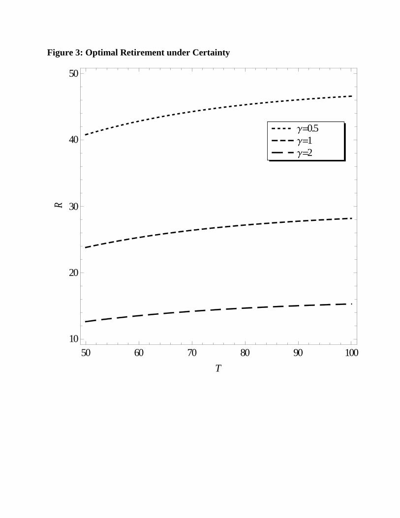
Figure 3: Optimal Retirement under Certainty
50 60 70 80 90 10010
20
30
40
50
T
R
210.5
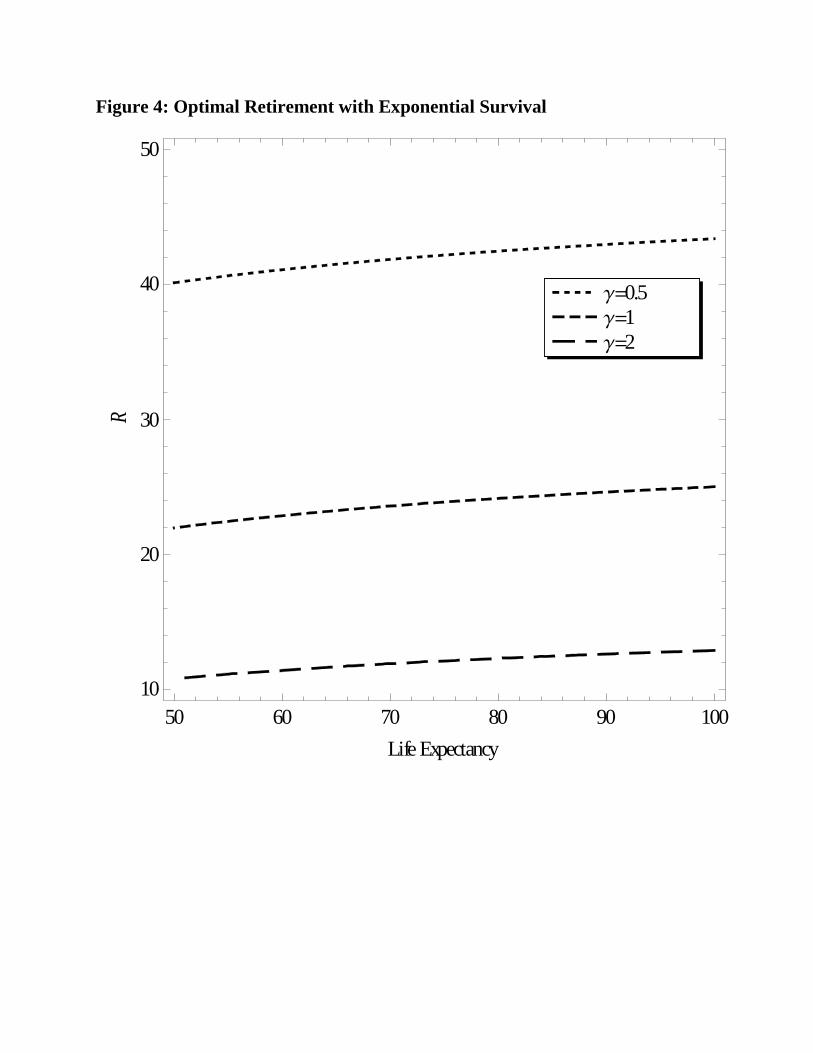
Figure 4: Optimal Retirement with Exponential Survival
50 60 70 80 90 10010
20
30
40
50
Life Expectancy
R
210.5
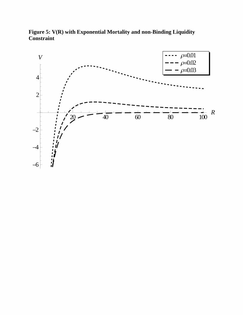
Figure 5: V(R) with Exponential Mortality and non-Binding Liquidity Constraint
20 40 60 80 100R
6
4
2
2
4
V
0.030.020.01
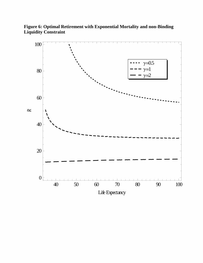
Figure 6: Optimal Retirement with Exponential Mortality and non-Binding Liquidity Constraint
40 50 60 70 80 90 1000
20
40
60
80
100
Life Expectancy
R
210.5
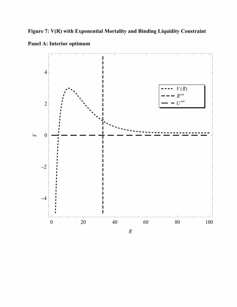
Figure 7: V(R) with Exponential Mortality and Binding Liquidity Constraint
Panel A: Interior optimum
0 20 40 60 80 100
-4
-2
0
2
4
R
V
U**R**V HRL
Panel B: Optimum at Infinity
0 20 40 60 80 100
-4
-2
0
2
4
R
V
U**R**V HRL
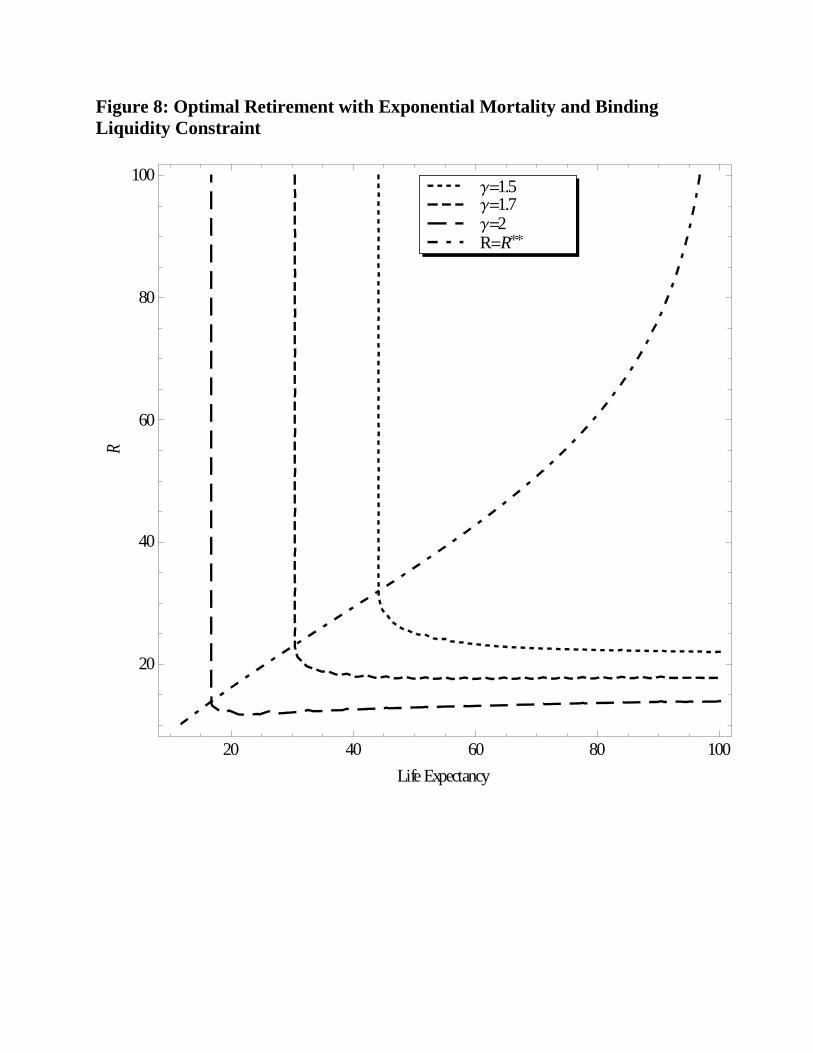
Figure 8: Optimal Retirement with Exponential Mortality and Binding Liquidity Constraint
20 40 60 80 100
20
40
60
80
100
Life Expectancy
R
RR21.71.5
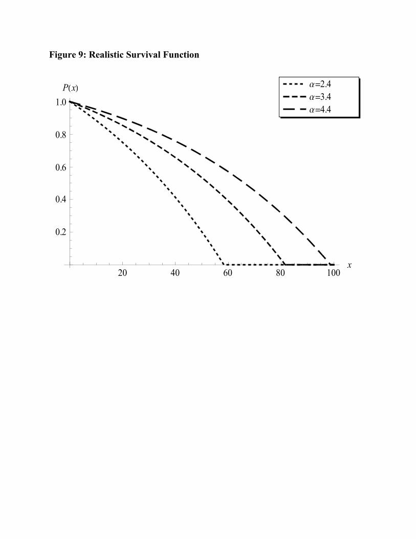
Figure 9: Realistic Survival Function
20 40 60 80 100x
0.2
0.4
0.6
0.8
1.0
PHxL
a=4.4
a=3.4
a=2.4
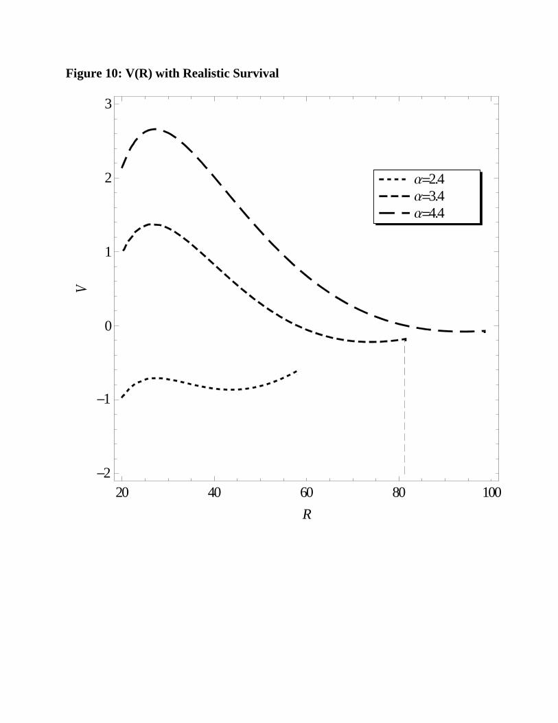
Figure 10: V(R) with Realistic Survival
20 40 60 80 1002
1
0
1
2
3
R
V
4.43.42.4
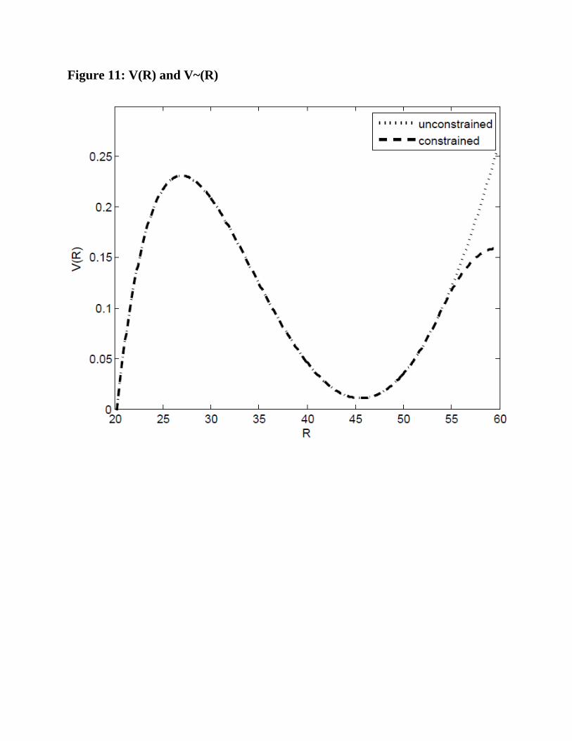
Figure 11: V(R) and V~(R)
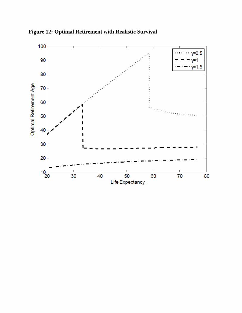
Figure 12: Optimal Retirement with Realistic Survival
1
1.5
2
Expe
cted
Utility
Figure 13: Expected Utility as a Function of Retirement Age
2000
1990
1980
1970
1960
1950
1940
1930
0
0.5
1
1.5
2
40 43 46 49 52 55 58 61 64 67 70 73 76 79 82 85 88 91 94 97 100
Expe
cted
Utility
Retirement Age
Figure 13: Expected Utility as a Function of Retirement Age
2000
1990
1980
1970
1960
1950
1940
1930
1920
1910
1900
1
1.5
2
Consum
ption
Figure 14: Optimal Consumption PathR*=57, Life Table=1980
0
0.5
1
1.5
2
20 23 26 29 32 35 38 41 44 47 50 53 56 59 62 65 68 71 74 77 80 83 86 89 92 95 98 101
104
107
110
113
116
119
Consum
ption
Age
Figure 14: Optimal Consumption PathR*=57, Life Table=1980
10
15
20
Aassets
Figure 15: Optimal Asset PathR*=57, Life Table=1980
0
5
10
15
20
20 23 26 29 32 35 38 41 44 47 50 53 56 59 62 65 68 71 74 77 80 83 86 89 92 95 98 101
104
107
110
113
116
119
Aassets
Age
Figure 15: Optimal Asset PathR*=57, Life Table=1980
1
1.5
2
Consum
ption
Figure 16: Optimal Consumption PathR*=∞, Life Table=1980
0
0.5
1
1.5
2
20 23 26 29 32 35 38 41 44 47 50 53 56 59 62 65 68 71 74 77 80 83 86 89 92 95 98 101
104
107
110
113
116
119
Consum
ption
Age
Figure 16: Optimal Consumption PathR*=∞, Life Table=1980
4
6
8
Aassets
Figure 17: Optimal Asset PathR=∞, Life Table=1980
0
2
4
6
8
20 23 26 29 32 35 38 41 44 47 50 53 56 59 62 65 68 71 74 77 80 83 86 89 92 95 98 101
104
107
110
113
116
119
Aassets
Age
Figure 17: Optimal Asset PathR=∞, Life Table=1980
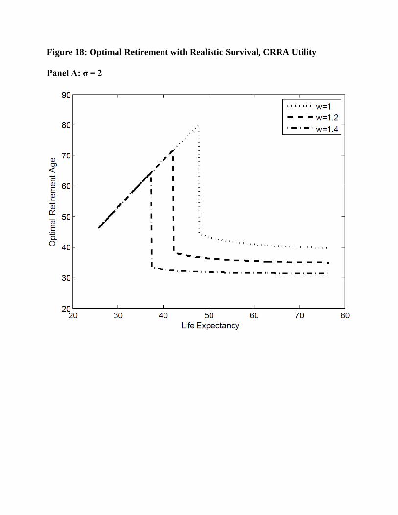
Figure 18: Optimal Retirement with Realistic Survival, CRRA Utility Panel A: σ = 2
Panel B: σ = 3
Panel C: σ = 4


![Photoelectric effect [45 marks] - Peda.net](https://img.pdfslide.us/doc/110x75/61869499ebec7b11d64c02eb/photoelectric-eect-45-marks-pedanet.jpg)