General rights Copyright and moral rights for the publications made accessible in the public portal are retained by the authors and/or other copyright owners and it is a condition of accessing publications that users recognise and abide by the legal requirements associated with these rights.

Users may download and print one copy of any publication from the public portal for the purpose of private study or research.

You may not further distribute the material or use it for any profit-making activity or commercial gain

You may freely distribute the URL identifying the publication in the public portal If you believe that this document breaches copyright please contact us providing details, and we will remove access to the work immediately and investigate your claim.

Downloaded from orbit.dtu.dk on: Feb 17, 2019

Morphology-based black and white filters for topology optimization

Sigmund, Ole

Published in:Structural and Multidisciplinary Optimization

Link to article, DOI:10.1007/s00158-006-0087-x

Publication date:2007

Document VersionEarly version, also known as pre-print

Link back to DTU Orbit

Citation (APA):Sigmund, O. (2007). Morphology-based black and white filters for topology optimization. Structural andMultidisciplinary Optimization, 33(4-5), 401-424. DOI: 10.1007/s00158-006-0087-x

Morphology-based black and white filters for topology optimization

Ole SigmundDepartment of Mechanical Engineering, Solid Mechanics

Technical University of DenmarkNils Koppels Alle, B. 404, DK-2800 Lyngby, Denmark

Tel.: (+45) 45254256, Fax.: (+45) 45931475email: sigmund@mek.dtu.dk

Lyngby November 9, 2006

Abstract

In order to ensure manufacturability and mesh-independence in density-based topology opti-mization schemes it is imperative to use restriction methods. This paper introduces a new class ofmorphology based restriction schemes which work as density filters, i.e. the physical stiffness of anelement is based on a function of the design variables of the neighboring elements. The new filtershave the advantage that they eliminate grey scale transitions between solid and void regions. Usingdifferent test examples, it is shown that the schemes in general provide black and white designs withminimum length-scale constraints on either or both minimum hole sizes and minimum structuralfeature sizes. The new schemes are compared with methods and modified methods found in theliterature.

Keywords: topology optimization, regularization, image processing, morphology operators, manu-facturing constraints.

1 Introduction

It is well-known that the standard “density approach to topology optimization” (Bendsøe, 1989; Sig-mund, 2001a) is prone to problems with checkerboards and mesh-dependency if no regularizationscheme is applied. As reviewed by Sigmund and Petersson (1998) a large number of works have sug-gested different regularization schemes to be used in connection with topology optimization. However,each scheme has its pros and cons and probably the ideal scheme still has to be invented.

In this paper, we present a new family of regularization schemes that are based on image morphologyoperators. Although the new schemes, as will be demonstrated, solve many of the known problemswith existing schemes, they require a continuation approach and hence are not very computationallyefficient, thus there is still room left for improvement.

Restriction methods for density based topology optimization problems can roughly be divided intothree categories: 1) mesh-independent filtering methods, constituting sensitivity filters (Sigmund,1994, 1997; Sigmund and Petersson, 1998) and density filters (Bruns and Tortorelli, 2001; Bourdin,2001); 2) constraint methods such as perimeter control (Ambrosio and Buttazzo, 1993; Haber et al,1994), global gradient control (Bendsøe, 1995; Borrvall, 2001), local gradient control (Niordson, 1983;Petersson and Sigmund, 1998; Zhou et al, 2001), regularized penalty methods (Borrvall and Petersson,2001) and integral filtering (Poulsen, 2003); and 3) other methods like wavelet parameterizations (Kimand Yoon, 2000; Poulsen, 2002), phase-field approaches (Bourdin and Chambolle, 2003; Wang andZhou, 2004) and level-set methods (Sethian and Wiegmann, 2000; Wang et al, 2003; Allaire et al,

1

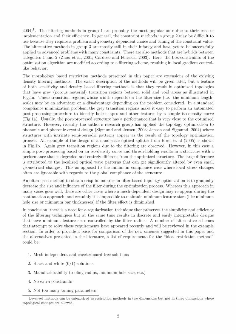
2004)1. The filtering methods in group 1 are probably the most popular ones due to their ease ofimplementation and their efficiency. In general, the constraint methods in group 2 may be difficult touse because they require a problem and geometry dependent choice and tuning of the constraint value.The alternative methods in group 3 are mostly still in their infancy and have yet to be successfullyapplied to advanced problems with many constraints. There are also methods that are hybrids betweencategories 1 and 2 (Zhou et al, 2001; Cardoso and Fonseca, 2003). Here, the box-constraints of theoptimization algorithm are modified according to a filtering scheme, resulting in local gradient control-like behavior.

The morphology based restriction methods presented in this paper are extensions of the existingdensity filtering methods. The exact description of the methods will be given later, but a featureof both sensitivity and density based filtering methods is that they result in optimized topologiesthat have grey (porous material) transition regions between solid and void areas as illustrated inFig.1a. These transition regions whose width depends on the filter size (i.e. the minimum length-scale) may be an advantage or a disadvantage depending on the problem considered. In a standardcompliance minimization problem, the grey transition regions make it easy to perform an automatedpost-processing procedure to identify hole shapes and other features by a simple iso-density curve(Fig.1a). Usually, the post-processed structure has a performance that is very close to the optimizedstructure. However, recently the author’s research group has applied the topology optimization tophononic and photonic crystal design (Sigmund and Jensen, 2003; Jensen and Sigmund, 2004) wherestructures with intricate semi-periodic patterns appear as the result of the topology optimizationprocess. An example of the design of a nano-scale optical splitter from Borel et al (2005) is shownin Fig.1b. Again grey transition regions due to the filtering are observed. However, in this case asimple post-processing based on an iso-density curve and thresh-holding results in a structure with aperformance that is degraded and entirely different from the optimized structure. The large differenceis attributed to the localized optical wave patterns that can get significantly altered by even smallgeometrical changes. This as opposed to the minimum compliance case where local stress changesoften are ignorable with regards to the global compliance of the structure.

An often used method to obtain crisp boundaries in filter-based topology optimization is to graduallydecrease the size and influence of the filter during the optimization process. Whereas this approach inmany cases goes well, there are other cases where a mesh-dependent design may re-appear during thecontinuation approach, and certainly it is impossible to maintain minimum feature sizes (like minimumhole size or minimum bar thicknesses) if the filter effect is diminished.

In conclusion, there is a need for a regularization technique that preserves the simplicity and efficiencyof the filtering techniques but at the same time results in discrete and easily interpretable designsthat have minimum feature sizes controlled by the filter radius. A number of alternative schemesthat attempt to solve these requirements have appeared recently and will be reviewed in the examplesection. In order to provide a basis for comparison of the new schemes suggested in this paper andthe alternatives presented in the literature, a list of requirements for the “ideal restriction method”could be:

1. Mesh-independent and checkerboard-free solutions

2. Black and white (0/1) solutions

3. Manufacturability (tooling radius, minimum hole size, etc.)

4. No extra constraints

5. Not too many tuning parameters1Level-set methods can be categorized as restriction methods in two dimensions but not in three dimensions where

topological changes are allowed.

2

b)

a)Result of simple post-processing

Density image as result of topology optimization

Figure 1: Demonstration of grey (porous) transition regions as results of topology optimization usingfiltering approaches. a) Grey scale picture of optimized MBB-beam with post-processed version basedon the 50% density contour curve. b) Grey scale picture of a photonic crystal splitter nano-opticaldevice.

3

6. Stable and fast convergence

7. General applicability

8. Simple implementation

9. Low CPU-time

Some comments should be attached to the list. Concerning item 1, a good scheme should resultin designs with smoothly varying geometries with details defined by the radius of the filter. Theneed for crisp black and white solution (item 2) was discussed above. Manufacturability (item 3) isclosely related to item 1 but also includes the avoidance of non-manufacturable features such as sharpcorners. Extra constraints (item 4) require difficult and problem dependent choice of constraint valuesand should be avoided. Tuning parameters (item 5) that are problem and geometry dependent shouldbe avoided. With ”stable convergence” (item 6) it is understood that the method is independent of theproblem formulation (and physical setting) and does not require delicate fine-tuning of parameters.With ”general applicability” (item 7) it is understood that the scheme should be applicable to problemsinvolving any kind of objective functions, constraints, density interpolation functions and physicalmodels. With ”simple implementation” (item 8) it is understood that one can use ”black-box” finiteelement codes and optimizers.

Depending on the viewpoint, the prioritized list may look different. The suggested list probablyapplies to researchers and academicians who are interested in getting as close to the global optimumas possible whereas software vendors may move ”stable and fast convergence” (item 6) and ”LowCPU-time” (item 9) up front as items 1 and 2, respectively.

In order to test and compare new and old filter methods this paper suggests three different test prob-lems. When performing a test and review of different filtering methods it is very difficult to perform afair comparison since every author has his preferred parameter settings, interpolation function, opti-mizer and test problems. A method may work very well in one problem setting or for one test problem,whereas it may fail in other settings. However, for a method to be generally stable and applicable, itshould be possible to use it in a standard setting. Hence, if a method does not work well for the threetest cases provided in this paper, it will probably not be working well for other formulations either.The three test cases are therefore not chosen arbitrarily but are carefully selected in order to exploitthe weaknesses of the different filtering methods with regards to the 9 requirements to an ideal filtermethod listed earlier.

The paper is organized as follows. In section 2 we set up the three test problems that will be used tobenchmark the performance of new and old filters. In section 3 we review and set up the equations forthe original sensitivity and density filters. In section 4 we present a new family of filtering techniquesbased on image morphology operators and in section 5 we briefly review black and white filteringalternatives from the recent literature. In section 6 we discuss implementation aspects and sensitivityanalysis for the new morphology based filter schemes. In section 7 we present, discuss and comparethe results obtained for the different approaches. Finally, we summarize our findings and try to drawsome general guidelines for the use of filtering methods in density based topology optimization insection 8.

2 Problem formulation and definition of test problems

In general, many new procedures and schemes in topology optimization are tested on simple compli-ance minimization problems with a material resource constraint. However, it is dangerous to drawgeneral conclusions from such studies since compliance minimization problems have some features thatmake them especially easy to solve. First of all, the compliance (objective) function is self-adjoint, i.e.

4

the direct solution and the adjoint solution are the same (possibly with opposite signs) and thus sen-sitivities will always have the same sign. Second, the single volume constraint is linear and monotonein the design variables providing for easy solution by optimality criteria approaches or other heuris-tic procedures. Nevertheless, we do include a compliance based test problem here (the MBB-beam)for comparison with the literature but we also use two other test cases that are harder to solve. Inthis connection, it should also be noted that some authors have used a two-bar truss example, i.e. avery short cantilever beam, as a test case for filtering schemes. The two-bar example (obviously) hasa unique solution (two bars) and thus demonstrating mesh independent solutions for this test casedemonstrates nothing.

A problem that is already much more difficult to solve than simple compliance minimization problemsis the design of a compliant force inverter (Sigmund, 1997, 2000). Here we use a simple formulation aspresented in Sigmund (2000) and Bendsøe and Sigmund (2003) that requires minimization of outputdisplacement subject to a single (linear) constraint on material resource. This problem is non-selfadjoint, meaning that the sensitivities of the objective function may take both positive and negativevalues – a feature that makes the convergence of this problem much more prone to local minima.

The third test case involves wave propagation and has no volume constraint. The latter feature dis-qualifies many of the existing filter approaches since they rely on an active material resource constraint.

The test cases are all based on the standard ”density based approach to topology optimization”, i.e.the design variables ρ represent piece-wise constant element densities. We consider linear isotropicmaterials and the Young’s modulus of an element is a function of the element design variable ρe givenby the modified SIMP (Simplified Isotropic Material with Penalization) interpolation scheme

Ee = E(ρe) = Emin + ρpe(E0 − Emin), ρe ∈ [0, 1], (1)

where p is the penalization power, Emin is the stiffness of soft (void) material (non-zero in order toavoid singularity of the stiffness matrix) and E0 is the Young’s modulus of solid material. Use of themodified SIMP scheme (1) as opposed to the standard SIMP scheme E(ρe) = ρp

eE0 with ρe ∈]0, 1] hasa number of advantages, including that the minimum stiffness value is independent of the penalizationfactor, that the modified formulation also covers two phase design problems and that the modified formis easier to generalize for use in the various filtering schemes discussed in the present paper. The teststructures are all discretized by 4-node bi-linear finite elements. Otherwise, the implementation is donein MATLAB as described in Sigmund (2001a). As the optimizer we use the MATLAB implementationof the Method of Moving Asymptotes (Svanberg, 1987) made freely available for research purposes byKrister Svanberg.

In the following we define the three problem specific formulations.

2.1 The MBB-beam

The optimization problem for the MBB-beam example may be written as

minρ

: f(ρ) = UTKU =∑e

uTe keue

s.t. : KU = F: g = V (ρ)/V ∗ − 1 =

∑e

veρe/V∗ − 1 ≤ 0

: 0 ≤ ρ ≤ 1

⎫⎪⎪⎪⎪⎪⎪⎬⎪⎪⎪⎪⎪⎪⎭

, (2)

where K, U and F are the global stiffness matrix, displacement vector and force vector, respectively,lower case symbols indicate element wise quantities, ke = k(ρe) = E(ρe)k0

e, is the element stiffnessmatrix, k0

e is the element stiffness matrix for unit Young’s modulus, the sum symbol in the first lineindicates finite element summation, V ∗ is the material resource constraint and ve is the volume of

5

element e. The sensitivity expressions are simply found as∂f∂ρe

= −uTe

∂ke∂ρe

ue,

∂ke∂ρe

= p (E0 − Emin)ρp−1e k0

e,

∂g∂ρe

= ve/V∗.

(3)

The design domain and its dimensions are shown in Fig. 2a. Due to symmetry we model only halfthe design domain which is discretized with 120 by 40 bi-linear quadrilaterals. The Young’s modulusof solid material is E0 = 1, the minimum stiffness is Emin = 10−9, the Poisson’s ratio is ν = 0.3, thefilter radius (see later) is R = 3.5 and the penalization factor is p = 3.

2.2 The compliant force inverter

In compliant mechanism design, a typical design goal is to transfer work from an input actuator to anoutput spring (cf. Sigmund, 2000). For the present case, we consider the force inverter that previouslyhas been used as a benchmark (Sigmund, 1997). The optimization problem for the force inverterexample may be written as

minρ

: f(ρ) = LTU

s.t. : KU = F: g = V (ρ)/V ∗ − 1 =

∑e

veρe/V∗ − 1 ≤ 0

: 0 ≤ ρ ≤ 1

⎫⎪⎪⎪⎪⎪⎬⎪⎪⎪⎪⎪⎭

, (4)

where L is a unit length vector with zeros at all degrees of freedom except at the output point whereit is one. The sensitivity is simply found as

∂f

∂ρe= λT

e

∂ke

∂ρeue, (5)

where λ is the global adjoint vector found by the solution of the adjoint problem Kλ = −L and λe

is the part of the adjoint vector associated with element e. The design domain and its dimensionsare shown in Fig. 2b. For faster computations we consider only half the structure due to symmetry.The design domain is discretized with 120 by 60 bi-linear quadrilaterals, the filter radius is R = 2.5,the input force is Fin = 1 and the input and output spring stiffnesses are kin = 1 and kout = 0.001,respectively. Otherwise, the parameters are the same as for the MBB example. Remark that the inputand output spring stiffnesses are chosen such that the resulting mechanism without filtering exhibitsso-called one-node-connected hinges. These are numerical artifacts related to checkerboard patternswhich for a compliant mechanism have the (artificial) advantage that they are good in transmittingforces but deliver no resistance to bending. For higher stiffness of the output spring, the hinge-likeconnection becomes more solid (distributed compliant) on the cost of smaller output displacement(Sigmund, 1997). In order to compare the different filtering methods abilities to prevent hinges, wehere select a small value of the output spring stiffness.

2.3 The wave transmitter

Recently, the topology optimization method has been applied to the design of wave-propagation prob-lems based on band gap structures both for phononic and photonic applications (Sigmund and Jensen,2003; Jensen and Sigmund, 2004). A special feature of these problems is that they require no volumeconstraint. An optimization problem for a wave transmitter example may be written as

minρ

: f(ρ) = −UTLU

s.t. :(K + iΩC − Ω2M

)U = F

: 0 ≤ ρ ≤ 1

⎫⎪⎬⎪⎭ , (6)

6

����

����

���� ���� ����

����

120

40

����

����

c)

1

��������������������������

1

120

60

����

����

b)

����

a)

����

���� ���� ����

����

?

?

������

������

����

������

������

������

������

��������

��������

������

������

������������

��������

?

kin kout

fin outu

������

�����

�����

����������

����������

?

Figure 2: Design domains and boundary conditions for the three test problems. a) The MBB-beam,b) the compliant force inverter and c) a wave focussing device

7

where L this time is a zero matrix with ones at the diagonal entries corresponding to the degrees offreedom where the wave amplitude is to be maximized, i is the complex operator and overbars meancomplex conjugate. M and C are the global mass and damping matrices, respectively. The globalmass matrix is defined as M =

∑e (�min + ρe(�0 − �min))m0

e, where �min and �0 are the specificmass densities of background material and foreground material, respectively, and m0

e is the elementmass matrix for unit specific mass density. In order to assure black and white solutions we apply theso-called ”pamping” (penalization damping) method introduced in Jensen and Sigmund (2005). Theglobal damping matrix is defined as C =

∑e qρe(1 − ρe)c0

e, where q is the pamping factor and c0e is

the element damping matrix (here mass proportional, i.e. c0e = m0

e). The pamping method ensuresblack and white solutions in wave transmission problems by introducing an (artificial) damping inintermediate density elements.

The sensitivity of the objective function is found as

∂f∂ρe

= 2�(λT

e

[∂ke∂ρe

+ iΩ∂ce∂ρe

− Ω2 ∂me∂ρe

]ue

),

∂ce∂ρe

= q(1 − 2ρe)m0e,

∂me∂ρe

= (�0 − �min)m0e,

(7)

where λ is the solution to the adjoint problem(K + iΩC− Ω2M

)Tλ = −LU and �(·) denotes the

real part of (·). In practice, the objective function for wave propagation problems may change byorders of magnitude during optimization which may cause normalization problems for the optimizer.Therefore, we optimize log(f) instead and the sensitivities are modified accordingly (i.e. ∂f/∂ρe

becomes (∂f/∂ρe)/f).

The design domain and its dimensions are shown in Fig. 2c. The design domain is discretized with 80by 80 bi-linear quadrilaterals, the filter radius is R = 2.5/80, the pamping coefficient is q = 5 and theangular frequency is Ω = 10. The material properties used mimic the stiffness and density ratios ofsteel and polyester, i.e. E0 = 1, Emin = 0.025, �0 = 1 and �min = 0.15. The structure is supportedby dampers perpendicular to the surfaces at all four edges with damping factors 0.1 and a distributedvertical input load (i.e. an incoming shear wave) on the left edge. The goal of the optimizationproblem is to maximize the vertical amplitude at the center node of the right edge, i.e. to obtain themost efficient shear wave focussing device.

3 Basic filtering methods

As discussed in the introduction, filtering methods intended for regularization of topology optimizationproblems can be divided into density and sensitivity based methods. In the former case, each elementdensity is redefined as a weighted average of the densities in a mesh-independent neighborhood ofthe element, before calling the finite element solver, and afterwards the sensitivities are modified in aconsistent way. In the latter case, the finite element problem is solved in the standard way but aftercalculating the sensitivities consistently, they are heuristically modified as weighted averages of thesensitivities in mesh-independent neighborhoods.

The neighborhood of element e, here named Ne, is generally specified by the elements that have centerswithin a given filter radius R of the center of element e, i.e.

Ne = {i | ||xi − xe|| ≤ R}, (8)

where xi is the spatial (center) location of element i.

In order to compare the different methods we perform different simplifications and generalizations.First, all methods are described in a discrete setting and density and sensitivity information is assumedconstant within each element and is evaluated in element centers. It is clear that especially for small

8

filter radius to mesh size ratios this simplification may cause unwanted effects that may distort theconclusions for the numerical results. Second, some of the filters from the literature are based ondensity interpolation schemes being different from piece-wise constant. Again, in order to make a fairand general comparison, these schemes are reformulated in the standard piece-wise constant densityform. It may be that this reformulation causes not so favorable behavior of the method, however, inorder to be generally applicable, the filtering method should also work in this setting.

A pitfall when working with filtering methods is the treatment of mesh boundaries. In principle oneshould expand the filter and include elements outside the mesh at external edges as void elementsand likewise one should expand the filter outside the mesh at symmetry edges and mirror the valuesfrom inside the mesh. Furthermore, supported or non-zero-traction boundaries should be specified tobe solid. In this way, one would obtain consistent filtering and avoid problems at edges and corners.However, no papers appear to have implemented such a scheme. Instead, it seems to be most commonsimply to perform the filtering operations only based on the elements inside the mesh. This is alsothe scheme applied here. As will be discussed later, the effect of the simplification seems to vary fromfilter scheme to filter scheme.

In the following two subsections, we discuss the two different filtering approaches in more detail.

3.1 Density filtering

Density filters work by modifying the element density and thereby stiffness to be a function of thedensities in a specified neighborhood of an element. The modified element density can be written as

ρ̃e = ρ̃e(ρi∈Ne), (9)

i.e., the modified element density ρ̃e is a function of the neighboring design variables ρi∈Ne . Hence,the modified stiffness in element e can be written as

Ee = Ee(ρ) = Ee(ρ̃e) = Emin + ρ̃pe(E0 − Emin), (10)

where ρ̃e is the filtered density. Several ways for implementing the density filtering have been proposedin the literature and the main ones will be reviewed below. Alternative density filter schemes will bereviewed in section 5.

An important characteristic of filter operators is volume-preservation, i.e. the volume of materialshould be the same before and after the filtering process. In practice, exact volume preservation isseldomly fulfilled due to boundary influence. Some of the suggested variations of the density filterthat have appeared in the literature do not preserve volume. This is no problem as long as the volumefraction constraint is modified accordingly and there are no fixed solid or void regions in the designdomain. For the present case, we are operating with a modified density function, hence the volumeconstraint must also be imposed on the modified (physical) density field. This means that the volumefraction constraint for a density filter approach must be defined as

g = V (ρ̃)/V ∗ − 1 =∑e

veρ̃e/V∗ − 1 ≤ 0 (11)

and not as g =∑e

veρe/V∗ − 1 as erroneously defined in some papers. The problem with non-volume

preserving filters and fixed solid or void regions will be discussed in the example section.

9

Basic density filtering

Density filtering was introduced by Bruns and Tortorelli (2001) and mathematically proven as a viableapproach by Bourdin (2001). The filtered density measure is

ρ̃e =

∑i∈Ne

w(xi)viρi

∑i∈Ne

w(xi)vi

, (12)

where the weighting function w(xi) is given by the linearly decaying (cone-shape) function

w(xi) = R − ||xi − xe|| (13)

as suggested in Bruns and Tortorelli (2001); Bourdin (2001). As defined earlier, vi denotes the volumeof element i.

In order to obtain a smoother weighting function, the Gaussian (bell shape) distribution function

w(xi) = e− 1

2

(||xi−xe||

σd

)2

(14)

was suggested in Bruns and Tortorelli (2003); Wang and Wang (2005) for use with the density filtering(12). In Bruns and Tortorelli (2003) the variance is defined by σd = R/3 and in Wang and Wang(2005) by σd = R/2. In both cases, the filter is truncated at radius R. For the latter case, it meansthat the bell-shape curve is heavily truncated. In tests, the author did not experience any advantagesof the smooth Gaussian function compared to the original linear function, however, it is possible thatthere is an advantage when the filtering scheme is used in connection with the element removal andre-introduction scheme suggested by Bruns and Tortorelli (2003).

For completeness one may also consider a constant weighting function

w(xi) = 1. (15)

together with the density filtering (12).

The effect of the weighting is highest for the constant weighting (15), less for the linear decayingweighting (13) and least for the Gaussian weighting (14). From a computing time point of view it isthus more efficient to use the constant weighting function (15) since a smaller filter radius will resultin the same filtering effect. In the comparison studies of the present paper, we will only present resultfor the linearly decaying weighting case (13).

When using density filters it is important to do the physically correct interpretation of the design. Inthe literature, this has sometimes caused problems although it should be rather simple. The originaldesign variables ρ have no physical meaning! They are only used as intermediate mathematicalvariables. Therefore, one should always show plots of the filtered design variables ρ̃ (the densitiesused in the SIMP-interpolation (10)), since they represent the physical density of the elements. Onecould also plot ρ̃p which would represent the physical stiffness of the elements. For historical reasonswe prefer the former case (i.e. we will plot the filtered densities ρ̃) but we also include plots of the(non-physical) design variable fields ρ for illustrative purposes.

3.2 Sensitivity filtering

Sensitivity filtering was introduced by Sigmund (1994, 1997); Sigmund and Petersson (1998) andhas become very popular both in academia and in commercial programs. The main idea is to basedesign updates on filtered sensitivities instead of the real sensitivities. Obviously, this is a simple but

10

potentially risky approach, especially for line-search based optimization schemes since the sensitivitydata may not represent a descent direction and hence the optimization may stop prematurely. However,numerous applications and multiple physics settings have proven the method very robust and reliableusing most of the popular optimization tools.

Original mesh-independent sensitivity filter

The original form of the sensitivity filter presented by Sigmund (1997) was

∂̃f

∂ρe=

∑i∈Ne

w(xi)ρi∂f

∂ρi

ρe

∑i∈Ne

w(xi), (16)

where the weighting function w(xi) is the linearly decaying function (13). When the lower boundon the design variable is 0 as it is here, ρe in the denominator of (16) should be substituted withmax(ρe, ε) where ε is a small number (e.g. 10−3).

A modification that accounts for non-regular meshes with varying element volumes ve is

∂̃f

∂ρe=

∑i∈Ne

w(xi)ρi∂f

∂ρi/vi

ρe/ve

∑i∈Ne

w(xi). (17)

Intuitively, it would have made more sense to multiply by the element volumes (big elements, bigweight and small elements, small weight), however, the motivation for dividing by the volumes ispartly based on numerical experiments and partly based on energy considerations. By dividing by theelement volume, the term inside the summation in the numerator can be interpreted as an averagedstrain energy density (energy per unit volume).

Through time, several researchers have tried to explain the exact workwise of the sensitivity filter, how-ever, so far without success. Since the sensitivities are modified heuristically, it is probably impossibleto figure out what objective function is actually being minimized but generally it may be stated thatthe filtered sensitivities correspond to the sensitivities of a smoothed version of the original objectivefunction. Despite that the sensitivities are modified in a heuristic way, the author has throughout hiscareer solved numerous different problems involving up to 20 filtered constraints without convergenceproblems. A key point behind the success of the method seems to be the scaling with the density inthe nominator and the denominator in (16). A number of modifications of the filter will be discussedin section 5.

4 Filtering based on image morphology operators

A common problem for the standard density and sensitivity filters discussed in the previous sectionis that a grey transition region between solid and void areas always will appear due to the averagingnature of the density filter operator. In the following, we will present a new scheme that prevents thegrey transition regions but (mostly) preserves the good features of the density filtering method.

In image analysis, morphology operators are used to quantify holes or objects, restore noisy picturesand perform automatic inspection of image data (Pratt, 1991). The basic morphology operators are“erode” and “dilate” and several extensions can be performed by sequentially applying the erode anddilate operators.

11

The work-wise of some basic binary morphology operators are illustrated in the following. An originalbinary image is shown in Fig. 3a. In image processing one defines a so-called “structuring element”which basically corresponds to the neighborhood operator defined in (8). Performing the morphologyoperation called erode, verbally corresponds to translating the center of the neighborhood over eachelement in the design domain. If any of the pixels covered by the neighborhood is void, then thecenter pixel is made void. Oppositely, the dilate operation sets the center pixel to solid if any pixelcovered by the neighborhood is solid. The “open” and “close” operations are defined as an erodefollowed by a dilate operation and a dilate followed by an erode operation, respectively. The resultsof the four different operations are seen in Fig. 3b-e. The erode and dilate operators are not volumepreserving. In particular, the erode operator removes any feature in the original image that is smallerthan the neighborhood (Fig. 3b). Oppositely, the dilate operator fills any hole that is smaller thanthe neighborhood (Fig. 3c). The open and close operators are volume preserving, have almost thesame behaviors as the erode and dilate operators, respectively, but retain the feature sizes above thefilter limit from the original image. Immediately, one recognizes that the morphology operators arewell suited to provide for feature size control in topology optimization, however, in order to makethem practically applicable, the min/max-type operators need to be redefined as continuous anddifferentiable functions. This is discussed in the following.

Dilate

In its discrete form the dilation operator is a max operator, i.e. the physical density of element etakes the maximum of the densities in the neighborhood Ne. The max-formulation is not suitable forgradient-based optimization hence it must be converted to a continuous form. A continuous form thatuses the Kreisselmeier and Steinhauser (1983) formulation can be formulated as

ρ̃e = log

⎛⎜⎜⎜⎝

∑i∈Ne

eβρi

∑i∈Ne

1

⎞⎟⎟⎟⎠ /β. (18)

For β approaching zero, the filter corresponds to the original density filter (12) with constant weighting(15) and for β approaching infinity it corresponds to the max-operator. In order to obtain a numeri-cally stable scheme β must be gradually increased using a continuation scheme. Based on numericalexperience, the continuation method is started with β = 0.2 and then gradually increased to 200.Note also that there is no volume dependence in the continuous morphology operator (18) due to itsoriginal max-operator nature.

It should also be noted here that the proposed continuation method maintains the filtering effect andis only used to enforce black and white solutions. This is in contrast to other continuation methodswhere the filtering effect gradually is diminished urging the design into a local (black and white)minimum. As will be seen in the example section, the filter works as a ”fixed radius deposition tool”,i.e. no details of the structure are smaller than a circular (deposition) tool with radius R.

As will be seen later, the resulting physical density distributions ρ̄ become quite nice and clear butthe extremely thin (has a low volume fraction) design variable structure ρ makes the physical densitydistribution very sensitive to even small variations in the design variables and may explain occasionalinstabilities during convergence.

Erode

The morphological opposite of dilation is erosion, which in its discrete form corresponds to a min-operator, i.e. the physical density of element e is the minimum of the densities in the neighborhood.

12

Erode

Dilate

Open

Structuringelement

Close

a)

b)

c)

d)

e)

Original image

Figure 3: Demonstration of basic image morphology operators. The size of the structuring elementis enlarged for illustrative purposes. a) Original image and 5 element structuring element (neighbor-hood). b) Result of erosion, c) result of dilation, d) result of open (erosion followed by dilation) ande) result of close (dilation followed by erosion).

13

As opposed to the dilation operator, the design variable field is very thick (has a high volume fraction)and thus less sensitive to variations in the design variables. The Kreisselmeier-Steinhauser formulationagain gives a continuous form of the min-operator

ρe = 1 − log

⎛⎜⎜⎜⎝

∑i∈Ne

eβ(1−ρi)

∑i∈Ne

1

⎞⎟⎟⎟⎠ /β. (19)

As before, the filter is implemented by a continuation approach. Also, the filter corresponds to theoriginal density filter (12) with constant weights (15) for β approaching zero and to the min operatorfor β approaching infinity. Again, the continuation method starts with β = 0.2 and gradually increasesto 200. Also, as will be seen in the examples, this filter works as a “machining constraint”, i.e. theresulting topology has no hole features that are smaller than a circle with radius R.

Neither the dilation filter nor the erosion filter are volume preserving. A small extension, however,resolves this issue as will be shown in the following.

Close

Dilation may be followed by erosion to form a morphological close operation. In image processing,this corresponds to filling in all details with dimensions smaller than the filter size. If we denote thedilation operation by tilde and the erosion operation with an overline, the equation for the filtereddensity becomes

ρ̃e = ρ̃e

(ρ̃j∈Ne(ρi∈Nj )

). (20)

Results obtained using the close filter are quite similar to those obtained using the dilation filteralthough the former seems to be a bit more stable due to the denser design variable field. The closeoperator is volume preserving.

Open

Likewise, erosion may be followed by dilation to form the open operator. In image processing, thiscorresponds to removing all details with dimensions smaller than the filter size. If we denote thedilation operation by tilde and the erosion operation with a bar, then the filtered density becomes

ρ̃e = ρ̃e

(ρj∈Ne

(ρi∈Nj ))

. (21)

Results obtained using the open filter are quite similar to those obtained using the erosion filteralthough the latter seems to be a bit more stable due to the denser design variable field. The openoperator is also volume preserving.

Further morphological operators

In order to obtain minimum hole size and minimum structural detail size simultaneously, one maycombine the open and close operators to form the close-open operator

˜̃ρe = ˜̃

ρe

(ρ̃i∈Ne

(ρ̃j∈Ni

(ρ̃k∈Nj

(ρl∈Nk))))

, (22)

or the open-close operator

˜̃ρe = ˜̃ρe

(˜̃ρi∈Ne

(ρ̃j∈Ni

(ρk∈Nj

(ρl∈Nk))))

, (23)

14

i.e., in both cases one has to perform four consecutive filter operations which in itself is not bad,however, the computational burden of the associated sensitivity analysis becomes immense. In prac-tice, the sensitivity of one element becomes a function of its neighbors, which are function of theirneighbors, and so on four times. This overwhelming task is much heavier than the solution of thefinite element problem (see later discussion). A shortcut may be initially to combine the open andclose operators by taking the average of them, i.e.

˜̃ρe ≈[ρ̃e + ρ̃e

]/2 =

[ρ̃e

(ρ̃j∈Ne(ρi∈Nj )

)+ ρ̃e

(ρj∈Ne

(ρi∈Nj ))]

/2. (24)

After convergence, one may use the real open-close or close-open operators to provide the final solution.The open-close, the close-open and the combination operator are all volume preserving.

5 Alternative black and white filtering schemes

Since the review article by Sigmund and Petersson (1998) a number of alternative filtering schemesthat claim black and white solutions have been published. In the following, we briefly review thesemethods. The methods are again categorized in density and sensitivity based methods.

5.1 Density filters

Modified density filtering

In order to obtain more discrete solutions than provided by the original density filter (12), Guo andGu (2004) have suggested a modification to (10) where they multiply the filtered density with theoriginal variable, i.e.

Ee = Ee(ρ) = Ee(ρ, ρ̃e) = Emin + ρeρ̃pe(E0 − Emin), (25)

where ρ̃e is given by (12) and the linear weighting function (13). The authors claim that theirmodification results in improved black and white (0/1) solutions, however, they only show picturesbased on the design variables ρ which have no physical meaning. For density filtering methods, thevector ρ should only be seen as a mathematical design variable; the physical density distribution tobe plotted is given by the filtered vector ρ̃. When the filtered densities are plotted for the examplesfrom the paper by Guo and Gu (2004) many grey elements are observed, hence the basic idea of themethod fails. There are two other problems with Guo and Gu’s implementation. First, they use theintegral over the design variable as volume constraint which again does not make physical sense sincetheir filter is non-volume preserving. However, the correct choice for the material volume constraintis not obvious for this case - but should probably be based on

∑e veρeρ̃e. Second, the filter does not

converge to the original SIMP scheme (10) for the radius R going to zero - it actually converges toρp+1

e . Due to these shortcomings, no results will be shown for this method.

Bi-lateral density filtering

Wang and Wang (2005) suggest a modification to (12), a so-called bi-lateral filter, which apart fromthe distance weighting also includes a density weighting

ρ̃e =

∑i∈Ne

w(xi)w̃(ρi)viρi

∑i∈Ne

w(xi)w̃(ρi)vi

, (26)

15

wherew̃(ρi) = e−

12

(ρi−ρe

σr

)2

. (27)

Here, the variance factor for the density dependent weighting function w̃ is σr ∈]0, 1]. For the caseof σr = ∞, this filter corresponds exactly to the original density filter (12) with Gaussian weighting(14) and for σr approaching zero, the effect of the filter is eliminated. Despite lots of effort it wasnot possible to reproduce the results of the paper by Wang and Wang (2005). The authors write thatthey use a continuation approach to obtain their results, however, no details are given concerningits implementation. In the present investigation the bi-lateral filter is implemented with a fixedvalue of σr = 1. A larger value causes further blurring of boundaries corresponding to the originalGaussian density filter (14) and a smaller value causes appearance of checkerboard patterns and mesh-dependency.

Density filtering with a Heaviside step function

In order to obtain 0/1 solutions, Guest et al (2004) have modified the original filter (12) with aHeaviside function such that if ρ̃e > 0 then the physical element density will become one and only ifthe filtered density ρ̃e = 0 will the physical density be zero. The Heaviside function is approximatedas a smooth function governed by the parameter β, thus the physical density ρ̄e becomes

ρ̄e = 1 − e−βρ̃e + ρ̃ee−β. (28)

For β equal to zero, this filter corresponds exactly to the original density filter (12) with linearlydecaying weighting (13). For β approaching infinity, the modification efficiently behaves as a max-operator, i.e. the density value of the center pixel is set equal to one if any of the pixels within theneighborhood is larger than zero. Note that Guest et al (2004) include an extra term in (28) in orderto ensure that the lower bound on the design variable is fulfilled. With the present modified SIMPinterpolation scheme (10), this extra term can be left out. It should also be noted that Guest et al(2004) propose to use a more elaborate scheme for the density interpolation. Instead of calculatingthe filtered density based on the element values within the neighborhood, the paper suggest to usemapped nodal design variables, which is reported to result in better numerical behavior. In orderto make a fair comparison of methods we here chose to use the standard element density approach.However, one may keep the idea of Guest et al (2004) in mind for improving convergence also for thenew morphology based schemes presented in this paper. The backside of the idea is the more compleximplementation that requires numerical integration for the computation of each of the element stiffnessmatrices instead of just computing one matrix that holds for all elements in a regular mesh using thestandard approach.

For stable convergence the filter is employed using a continuation approach where the value of β isgradually increased from 1 to 500.

The scheme is very similar to the suggested dilate filter operator (18) described in the previous section.Basically, the difference lies in the implementation of the max operator. In the erode scheme, the centerpixel is defined as the direct maximum of the neighborhood pixels. In the Heaviside approach, thecenter pixel is set equal to zero if any of the pixels in the neighborhood is bigger than zero. For adiscrete image the two filters are equal but for continuous design variables, the schemes will behavedifferently.

Modified density filtering with a Heaviside step function

As was the case for the erosion operator compared to the dilation operator, one may reformulate theidea from Guest et al (2004) discussed above, to turn it into a min-operator based scheme instead ofa max-operator based scheme.

16

We reformulate the Heaviside operator to give zero density for ρ̃e < 1 and only density one for ρ̃e = 1,i.e. basically the center pixel only takes the value one if all neighboring elements have density one.The modified Heaviside step function is approximated as a smooth function again governed by theparameter β

ρ̄e = e−β(1−ρ̃e) − (1 − ρ̃e)e−β . (29)

For β equal to zero, this filter corresponds exactly to (12). For β approaching infinity, the Heavisidefunction is obtained. The structure corresponding to the design variables is in this case much thickerthan the physical structure, thus providing more stability during iterations. Also, as will be seen inthe examples, this filter works as a “machining” constraint, i.e. the resulting topology has no holefeatures that are smaller than a circle with radius R.

Both the direct Heaviside density filter and the modified version are non-volume preserving. However,in the spirit of the morphology operators, one could combine the two Heaviside filters to produce closeand open operators and thereby get volume preservation and other qualities. This idea, however, hasnot been tested here and will be left for future research.

5.2 Sensitivity filters

In the following three modifications of the original sensitivity filter (16) that may be simpler to explainare presented. In general, however, these modified sensitivity filters seem to be less stable as will beseen in the example section.

Alternative sensitivity filter

In order to obtain a more discrete (black and white) solution than for the original sensitivity filter(16), Borrvall (2001) suggests the following modification

∂̃f

∂ρe=

∑i∈Ne

w(xi)ρi∂f

∂ρi∑i∈Ne

ρiw(xi), (30)

i.e., the density weighting in the denominator is moved inside the summation. The effect of thismodification is more black and white solutions at the cost of loss of some mesh-independency effectas will be shown later.

Sensitivity filter without density weighting

In order to ensure symmetric behavior for multi-phase design problems, the author has previously(Sigmund, 2001b) suggested to drop the density weighting of the original sensitivity filter (16)

∂̃f

∂ρe=

∑i∈Ne

w(xi)∂f

∂ρi∑i∈Ne

w(xi). (31)

As for the alternative sensitivity filter above, this modification is introduced at the cost of loss of someof the filtering effect and will thus not be tested for the two-phase problems considered in this paper.

17

Mean sensitivity filter

One may also drop the distance weighting of the filter above and simply modify the sensitivities ofelement e to become the mean value of the neighboring sensitivities

∂̃f

∂ρe=

∑i∈Ne

∂f

∂ρi∑i∈Ne

1. (32)

As will be seen in the example section, this filter works surprisingly well in many cases, however,occasionally, especially for more advanced design problems than compliance minimization, it fails inproducing checkerboard-free and mesh-independent designs.

Bi-lateral sensitivity filter

This alternative filter (indirectly2) proposed in Wang and Wang (2005) is the same as (26), exceptthat the density outside the weighting functions is interchanged with the sensitivity, i.e.

∂̃f

∂ρe=

∑i∈Ne

w(xi)w(∂f

∂ρi)vi

∂f

∂ρi∑i∈Ne

w(xi)w(∂f

∂ρi)vi

(33)

where the sensitivity weighting is defined as

w(∂f

∂ρi) = e

− 12

( ∂f∂ρi

− ∂f∂ρe

σr

)2

. (34)

Here the variance factor is σr ∈]0, 1]. In contrast to the bi-lateral density filter (26), the author wasable to reproduce the examples from Wang and Wang (2005) for the bi-lateral sensitivity filter (33).However, for alternative design problems, such as modelling half the MBB-beam instead of the fullbeam, the scheme did not result in smooth and mesh-independent results. A two-bar truss problemwas also used as a test problem in the paper. Here it was also possible to reproduce the results,even using half the design domain due to symmetry, however, it does not seem justified to provemesh-convergence for a design problem that is known to have a unique (two-bar) solution.

6 Implementation of morphology based filters

Contrary to what one might expect it is not very complicated to implement density based filters in astandard topology optimization software and they may be implemented using black box finite elementsolvers. Also, the extensions to the morphology-based filters are straightforward.

In order to demonstrate the implementation we first show how the procedure works for the simpleoriginal density (12), the dilate (18) and the erode (19) filters.

The sensitivity of an (objective) function f with respect to a change in design variable ρe is found byuse of the chain rule

∂f

∂ρe=

∑i∈Ne

∂f

∂ρ̃i

∂ρ̃i

∂ρe, (35)

2Many of the examples in the paper are apparently run with this modified filter although the equation is not givenexplicitly.

18

where the sensitivity of the filtered density ρ̃i with respect to a change in design variable ρe is foundas

∂ρ̃i

∂ρe=

w(xe)ve∑j∈Ni

w(xj)vj

, (36)

for the original density filter (12). In the case of the dilate operator (18), the sensitivity of the filtereddensity becomes

∂ρ̃i

∂ρe=

eβρe∑j∈Ni

eβρj. (37)

The sensitivity expression for the close operator is similar to (37) with ρk interchanged with 1−ρk. Thesensitivity expressions for the open and close operators become a bit more involved and are discussedlater.

The main computational burden of the simple filtering schemes (the original density filter and thedilate and erode operators) is to find the neighbors to each element. This is especially true in thecase of irregular meshes. Therefore, we suggest to compute a “neighborhood” matrix N that containsrows with neighbors to each element in the structure once and for all before the optimization begins.Following this idea, a very simplified flow chart in pseudo code may look like

1. Build neighborhood matrix N

2. Initialize design variable vector ρ, counter iter=0 and change=1

3. while change>0.01 and iter ≤ 1000

4. iter = iter + 1

5. Compute filtered densities ρ̃ using (12) (or (18) or (19))

6. Solve FE problem based on filtered sensitivities ρ̃

7. Calculate intermediate sensitivities based on filtered densities, i.e.

∂f

∂ρ̃e= −uT

e

∂ke

∂ρ̃eue − pρ̃p−1

e uTe k0

eue (38)

8. Compute final sensitivities from (35) using (36)

9. Update design variables ρnew using MMA

10. Calculate change = ||ρnew − ρ||∞11. end

For the filters involving β continuation schemes, the value of β is initialized in step 2 and step 9 issubstituted with

9. if { ’mod(iter,50)=1’ or ’change<0.01’ and ’β ≤ βmax’ } thenβ = 2βchange = 0.5

end

19

where βmax is the maximum value of β which is 200 for the morphology schemes and 500 for theHeaviside schemes.

Only general guidelines for the sensitivity analysis for the more complex morphology operators willbe given in the following. For the simple erode and dilate schemes, the sensitivity of the objectivefunction can be written as equation (35) with (37), as discussed above. For the close (combined dilateand erode) operator it expands to

∂f

∂ρe=

∑i∈Ne

∑j∈Ni

∂f

∂ρ̃j

∂ρ̃j

∂ρ̃i

∂ρ̃i

∂ρe. (39)

The sensitivity of the open operator is obtained by switching tilde and bars. For the close-openoperator, the sensitivity expression expands to

∂f

∂ρe=

∑i∈Ne

∑j∈Ni

∑k∈Nj

∑l∈Nk

∂f

∂˜̃ρl

∂˜̃ρl

ρ̃k

∂ρ̃k

ρ̃j

∂ρ̃j

∂ρ̃i

∂ρ̃i

∂ρe. (40)

It is seen that the computational burden is growing immensely for the combined open-close andclose-open schemes. Assuming a design domain discretized by a thousand elements, a neighborhoodcomprising 9 elements and ignoring boundary effects, the number of filter summation operations forthe simple erode or dilate filters is 9,000, for the open and close filters it is 81,000 and for the open-close and close-open filters it is 6,561,000. The general expressions for the number of summationoperations for the three cases is size(Ne)n, size(Ne)2n and size(Ne)4n, respectively, where n is thenumber of design elements and Ne is the neighborhood of element e. For a more realistic (but stillrather academic) problem like the MBB test example considered in this paper, size(Ne) = 37 andn = 4800. This results in 9 × 109 summation operations. This number should be compared to anestimate of bw2 × ndof multiplication for the decomposition of a symmetric band matrix, where bwis the bandwidth of the stiffness matrix and ndof is the number of degrees of freedom. In the MBBtest example this corresponds to approximately 70 × 106 multiplication, i.e. a factor of at least 100times less than for the filter operation. In conclusion, the open-close and close-open filters are notpractically applicable in large scale problems. However, as will be demonstrated in the example sectionit is plausible to use the combined filter (24) (with a summation count of 6×106 for the MBB-example)until convergence followed by a few iterations with the full open-close or close-open filters to obtainreasonable designs with minimum feature size control for both holes and structural details.

7 Test of the filters

It is difficult to make a fair comparison of the different filter methods. For sure, the efficiency of eachfilter has been optimized by the respective authors and fine-tuning of involved parameters may beimportant. In the following, we test the different filters with standard parameters for the three testproblems. The main aim is to test and compare the different filters for their stability and efficiencyfor practical applications. If a filter technique requires too much fine-tuning of parameters to workwell on a specific example, it will anyway not be worthwhile using it in practice.

All the filters have been implemented in a MATLAB setting and are solved using MMA (Svanberg,1987) with standard settings. Each test example is run using 15 different filtering schemes and theresults are presented in figures and tables. As discussed earlier, we plot both the non-physical designvariable distribution ρ and the physical density distribution ρ̃ (the densities used in the SIMP inter-polation scheme (10)) in all figures. For the physical interpretation of a design, it is obviously thelatter plot that must be consulted. In order to have a “measure of discreteness”, i.e. a way to tell

20

Filter type Eq. Fig. f V/V ∗ Mnd (%) It.No filtering - 4a 196.8 0.5 1.45 50Standard filtersDensity w. lin. weight (12),(13) 4b 218.3 0.5 24.02 1000Bi-lateral density (26) 4c 213.6 0.5 21.92 73Heaviside (28) 4d 190.0 0.5 0.36 489Modified Heaviside (29) 4e 192.3 0.5 0.23 435Sensitivity (17) 4f 210.0 0.5 20.41 119Mean sensitivity (32) 4g 192.5 0.5 0.48 1000Bi-lateral sensitivity (33) 4h 186.6 0.5 0.89 225New morphology-based filtersDilate (18) 5a 192.9 0.5 2.24 532Erode (19) 5b 197.3 0.5 1.42 474Close (20) 5c 195.4 0.5 1.19 414Open (21) 5d 192.9 0.5 1.84 423Combi (24) 5e 194.6 0.5 1.71 425Close-Open (22) 5f 196.2 0.5 2.31 (444)Open-Close (23) 5g 196.2 0.5 2.50 (439)

Table 1: Results for the MBB example.

whether an optimized design has converged to a discrete solution, we introduce the measure

Mnd =

n∑e=1

4ρ̃e(1 − ρ̃e)

n× 100%. (41)

If a converged design is fully discrete, i.e. there are no elements with intermediate density values, Mnd

is 0(%). If the design is totally grey, i.e. all elements densities are equal to 0.5, Mnd is 100(%). Hence,the measure may be called a Measure of Non-Discreteness (Mnd).

In the following, we discuss the results for the three different test cases.

7.1 The MBB test example

The results for the MBB test example are shown in Figs. 4 and 5 and the data for the results aregiven in Tab. 1.

An examination of Figs. 4 and 5 reveals that the resulting topologies may be very different for thevarious filters even though the filter radius R is the same. However, the cases which do not correspondto the simple MBB topology in Fig. 4b are the cases where the filter radius is not directly connectedwith topological features. If our goal is to select methods that impose minimum length-scales andmanufacturability, we can at this point already dispose of the two Bi-lateral filter methods (Figs. 4cand h) and possibly the mean sensitivity filter (Fig. 4g). The rest of the topologies are very similarwith the exceptions of the original density filter result (Fig. 4b) and the sensitivity filter result (Fig.4f) which (as expected) show grey transitions between the solid and void regions. These filter-enforcedgrey regions are also reflected in the obtained compliances that are approximately 10% higher thanfor the discrete designs.

The results for the Heaviside (Fig. 4d), dilate (Fig. 5a) and open (Fig. 5d) filters are very similar.It is seen that the filters correspond to deposition tools, i.e. there are no structural details below the

21

h) Bi-lateral sensitivityg) Mean sensitivity

b) Density w. lin. weight

Filter size

a) No filtering

d) Heavisidec) Bi-lateral density

e) Modified Heaviside f) Sensitivity

Figure 4: Results for the MBB test example with standard filters. For each filter, two images areshown. The upper one shows the (non-physical) design variable field ρ and the lower one shows thefiltered (physical) density field ρ̃. a) No filtering, b) Density filter with linearly decaying weighting(12), (13), c) Bi-lateral density filter (26), d) Density filter with a Heaviside step function (28), e)Modified density filter with a Heaviside step function (29), f) Original sensitivity filter (17), g) Meansensitivity filter (32) and h) Bi-lateral sensitivity filter (33).

22

e) Combi f) Close-Open

g) Open-Close

Filter size

a) Dilate b) Erode

d) Openc) Close

Figure 5: Results for the MBB test example with new morphology based filters. For each filter, twoimages are shown. The upper one shows the (non-physical) design variable field ρ and the lower oneshows the filtered (physical) density field ρ̃. a) Dilate filter (18), b) Erode filter (19), c) Close filter(20), d) Open (21), e) Combination of the Close and Open filters (24), f) Close-Open filter (22) andg) Open-Close filter (23).

23

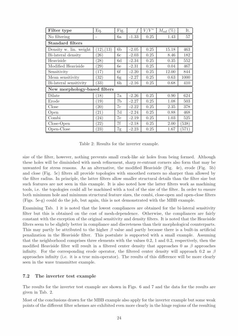
Filter type Eq. Fig. f V/V ∗ Mnd (%) It.No filtering - 6a -1.33 0.25 1.43 57Standard filtersDensity w. lin. weight (12),(13) 6b -2.05 0.25 15.18 463Bi-lateral density (26) 6c -2.03 0.25 8.46 182Heaviside (28) 6d -2.34 0.25 0.35 552Modified Heaviside (29) 6e -2.31 0.25 0.04 467Sensitivity (17) 6f -2.20 0.25 12.00 844Mean sensitivity (32) 6g -2.27 0.25 0.63 1000Bi-lateral sensitivity (33) 6h -2.16 0.25 0.68 410New morphology-based filtersDilate (18) 7a -2.26 0.25 0.90 624Erode (19) 7b -2.27 0.25 1.08 503Close (20) 7c -2.22 0.25 2.35 378Open (21) 7d -2.24 0.25 0.88 468Combi (24) 7e -2.19 0.25 1.03 525Close-Open (22) 7f -2.18 0.25 2.00 (538)Open-Close (23) 7g -2.23 0.25 1.67 (571)

Table 2: Results for the inverter example.

size of the filter, however, nothing prevents small crack-like air holes from being formed. Althoughthese holes will be diminished with mesh refinement, sharp re-entrant corners also form that may beunwanted for stress reasons. As an alternative, the modified Heaviside (Fig. 4e), erode (Fig. 5b)and close (Fig. 5c) filters all provide topologies with smoothed corners no sharper than allowed bythe filter radius. In principle, the latter filters allow smaller structural details than the filter size butsuch features are not seen in this example. It is also noted how the latter filters work as machiningtools, i.e. the topologies could all be machined with a tool of the size of the filter. In order to ensureboth minimum hole and minimum structural feature sizes, the combi, close-open and open-close filters(Figs. 5e-g) could do the job, but again, this is not demonstrated with the MBB example.

Examining Tab. 1 it is noted that the lowest compliances are obtained for the bi-lateral sensitivityfilter but this is obtained on the cost of mesh-dependence. Otherwise, the compliances are fairlyconstant with the exception of the original sensitivity and density filters. It is noted that the Heavisidefilters seem to be slightly better in compliance and discreteness than their morphological counterparts.This may partly be attributed to the higher β value and partly because there is a built-in artificialpenalization in the Heaviside filter. This postulate is supported with a small example. Assumingthat the neighborhood comprises three elements with the values 0.2, 1 and 0.2, respectively, then themodified Heaviside filter will result in a filtered center density that approaches 0 as β approachesinfinity. For the corresponding erode operator, the filtered center density will approach 0.2 as βapproaches infinity (i.e. it is a true min-operator). The results of this difference will be more clearlyseen in the wave transmitter example.

7.2 The inverter test example

The results for the inverter test example are shown in Figs. 6 and 7 and the data for the results aregiven in Tab. 2.

Most of the conclusions drawn for the MBB example also apply for the inverter example but some weakpoints of the different filter schemes are exhibited even more clearly in the hinge regions of the resulting

24

g) Mean sensitivity h) Bi-lateral sensitivity

Filter size

b) Density w. lin. weighta) No filtering c) Bi-lateral density

f) Sensitivitye) Modified Heavisided) Heaviside

Figure 6: Results for the inverter test example with standard filters. For each filter, two images areshown. The upper one shows the (non-physical) design variable field ρ and the lower one shows thefiltered (physical) density field ρ̃. a) No filtering, b) Density filter with linearly decaying weighting(12), (13), c) Bi-lateral density filter (26), d) Density filter with a Heaviside step function (28), e)Modified density filter with a Heaviside step function (29), f) Original sensitivity filter (17), g) Meansensitivity filter (32) and h) Bi-lateral sensitivity filter (33).

25

f) Close-Open

g) Open-Close

Filter size

a) Dilate b) Erode c) Close

d) Open e) Combi

Figure 7: Results for the inverter test example with new morphology based filters. For each filter, twoimages are shown. The upper one shows the (non-physical) design variable field ρ and the lower oneshows the filtered (physical) density field ρ̃. a) Dilate filter (18), b) Erode filter (19), c) Close filter(20), d) Open (21), e) Combination of the Close and Open filters (24), f) Close-Open filter (22) andg) Open-Close filter (23).

26

Filter type Eq. Fig. f V/V ∗ Mnd (%) It.No filtering - 8a -5.78 0.53 16.25 1000Standard filtersDensity w. lin. weight (12),(13) 8b -5.42 0.71 22.67 566Bi-lateral density (26) 8c -5.57 0.70 19.19 539Heaviside (28) 8d -6.55 0.90 0.87 563Modified Heaviside (29) 8e -6.45 0.28 1.06 856Sensitivity (17) 8f -6.32 0.90 4.81 929Mean sensitivity (32) 8g -6.37 0.81 3.45 635Bi-lateral sensitivity (33) 8h -6.31 0.63 10.29 643New morphology-based filtersDilate (18) 9a -5.86 0.88 2.75 694Erode (19) 9b -5.18 0.63 4.96 867Close (20) 9c -4.97 0.79 5.30 652Open (21) 9d -5.31 0.83 1.87 606Combi (24) 9e -5.25 0.80 4.46 839Close-Open (22) 9f -5.09 0.81 5.81 (1147)Open-Close (23) 9g -4.84 0.86 4.53 (1164)

Table 3: Results for the wave transmitter test example.

inverter topologies. As mentioned in Section 2, a weak point of the topology optimization methodin its application to compliant mechanism design is the modelling and design of hinges. Basically,the optimizer wants to make optimal but non-physical one-node connected hinges that can transferforces without bending resistance. The problem is mostly due to modelling issues. In reality, infinitestresses would appear in the hinges which would then fail. In order to prevent this, stresses in thehinge regions should be modelled correctly with higher order elements and mesh-refinement and stressconstraints should be imposed. However, this is impractical and may not resolve the problem entirely.Ideally a filter should take care of the problem but as is seen in Figs. 6 and 7 most of the filters donot. The only filter schemes that result in slender non-corner-connected hinges and discrete resultsare the modified Heaviside, close, combi and close-open filters (Figs. 6e, 7c, e and f). In principle,the dilate, open, open-close and Heaviside filters should also prevent the hinges with mesh-refinement,however, due to the staircase nature of the neighborhood region, it is often possible for the optimizerto find topologies where two circle like regions are only touching in one corner, resulting in a one-nodeconnected hinge. Defining the design variables in the nodal points (as in Guest et al (2004)) mayrelieve the problem although it has not been tested.

Judging from the objective function in Tab. 2 it is clear that all the discrete filters perform almostequally well with the hinge-preventing schemes (close, close-open and combi) being a bit worse sincethe distributed hinges are structurally non-efficient (with the finite element model applied). Again,the Heaviside filter result in more discrete solutions for the reasons discussed under the MBB example.

7.3 The wave transmitter test example

The results for the wave transmitter test example are shown in Figs. 8 and 9 and the data for theresults are given in Tab. 3.

Due to the non-existing volume constraint and the special nature of wave propagation problems, thetransmitter example really exhibits the differences between filters. Examining the result plots in Figs.8 and 9 and Tab. 3 it is clear that topologically extremely different structures may have very similar

27

g) Mean sensitivity h) Bi-lateral sensitivity

Filter size

a) No filtering b) Density w. const. weight c) Bi-lateral density d) Heaviside

e) Modified Heaviside f) Sensitivity

Figure 8: Results for the wave transmitter test example with standard filters. For each filter, twoimages are shown. The upper one shows the (non-physical) design variable field ρ and the lower oneshows the filtered (physical) density field ρ̃. a) No filtering, b) Density filter with linearly decayingweighting (12), (13), c) Bi-lateral density filter (26), d) Density filter with a Heaviside step function(28), e) Modified density filter with a Heaviside step function (29), f) Original sensitivity filter (17),g) Mean sensitivity filter (32) and h) Bi-lateral sensitivity filter (33).

28

f) Close-Open g) Open-Close

b) Erodea) Dilate

e) Combi

Filter size

c) Close d) Open

Figure 9: Results for the wave transmitter test example with new morphology based filters. For eachfilter, two images are shown. The upper one shows the (non-physical) design variable field ρ and thelower one shows the filtered (physical) density field ρ̃. a) Dilate filter (18), b) Erode filter (19), c)Close filter (20), d) Open (21), e) Combination of the Close and Open filters (24), f) Close-Open filter(22) and g) Open-Close filter (23).

29

objective function values which means that we are dealing with an optimization problem with a highlynon-unique solution. It is also clear that filtering is absolutely essential for getting any structurallyinterpretable design.

For the black and white filters, the results can be divided into the dilate-type filters with minimumstructural detail size but very small hole (epoxy) features, i.e. the Heaviside (Fig. 8d), dilate (Fig. 9a)and open (Fig. 9d) filters; the erode-type filters with minimum hole sizes, i.e. the modified Heaviside(Fig. 8e), erode (Fig. 9b) and close (Fig. 9c) filters; and the filters that take care of both minimumhole and structural sizes, i.e. the combi (Fig. 9e), close-open (Fig. 9f) and open-close (Fig. 9g).Again, the Heaviside filters result in the best objective function values. Their superiority in providingdiscrete designs is more clear in the present case where the morphology filters exhibit some problemswith intermediate density features. Although this problem could be resolved by raising the pampingparameter, the Heaviside filters are to be preferred here, since they have a “built-in” discretenesswhich diminishes the need for the penalization and/or pamping of intermediate densities.

7.4 Summary of examples

The only filters that have worked well for all examples are the new morphology and the Heavisidefilters. In all cases, the Heaviside filters have provided the best and most discrete designs, tightlyfollowed by the morphology based schemes. The alternative black/white filters like the two bilateralfilters, and the mean sensitivity filters may in many cases provide nice black and white solutions, butthere is no enforcement of a strict length-scale, hence they cannot be recommended as general purposefilters.

In many cases it is fine to work with the non-volume preserving filters such as the Heaviside filters,and the dilate and erode filters. However, if there are fixed solid or void regions involved in the designproblems which was not demonstrated in the three test cases, it is preferable to work with volumepreserving filters (such as the open or close filters). The reason is that details with features smallerthan the neighborhood area may appear at boundaries adjacent to the passive regions as illustratedin Fig. 10.

In conclusion, we recommend the open and close filters as stable and general filters which still arecomputationally efficient. The sensitivity analyses for the open-close and close-open operators are veryCPU-time consuming and cannot be recommended for general use. However, the combined scheme(24) composed as the average of the open and close operators constitutes a satisfactory replacement.

The reason for not directly recommending the Heaviside schemes is that they are not volume preservingand hence fail to provide length-scale constraints for the fixed solid/void domain case as discussedabove. However, it should be plausible to combine the Heaviside schemes into “Heaviside close andopen” morphological schemes just as done for the open and close operators. Although not tested here,the author believes that this idea will be rewarding with respect to computational stability and theenforcement of black and white solutions. This will also avoid the need for the special precautionsin the β-continuation approach discussed in Guest et al (2004), since the filters now become volumepreserving.

Finally, it should be mentioned that all the proposed filters can be applied to nodal-based designvariables as well. In fact this has been tested by the author for the MBB example with the sameconclusions as above and the results have therefore been omitted from the paper.

8 Conclusions

This paper has suggested a new family of morphology based density filtering schemes for topologyoptimization that provides mesh-independent, discrete and manufacturable solutions. The methods

30

erode

close

b)

c)

Neigborhood/Structuring element

~ρ

ρ~_

Des

ign

dom

ain

Fixe

d so

lid d

omai

nFi

xed

solid

dom

ain

Fixe

d so

lid d

omai

n

a)

ρ

ρ

Fixe

d so

lid d

omai

nFi

xed

solid

dom

ain

Figure 10: Demonstration of problems with non-volume-preserving filters and fixed solid domains. a)Design domain with fixed solid region and indication of neighborhood size. b) Left: image of designvariable field and right: filtered density field after erosion operation. The width of the lower hole issmaller than the neighborhood diameter. c) Left: image of design variable field and right: filtereddensity field after close operation. The small scale lower hole has been eliminated using the close filterwhich is volume preserving.

31

have been tested on three different test examples and have been compared with methods and modifiedmethods from the literature.

With the check list in section 1 in mind, it must be concluded that the new morphology based filterstogether with the Heaviside filters provide interesting new methodologies for topology optimizationwith manufacturing constraints. The only check point that is not fulfilled is point 6: “Stable and fastconvergence”. Due to the required continuation approach for the β parameter, the proposed methodstypically use between 500 and 1000 iterations to converge. Whereas this number may be satisfactoryfrom an academic point of view, it will not be accepted for industrial applications, hence the idealrestriction method probably still remains to be invented.

As a suggestion for future work, it is recommended to implement and test the extension of the Heav-iside filters (basic version proposed in Guest et al (2004)) to be used as morphology operators, i.e.sequentially applying the Heaviside and the modified Heaviside schemes in order to make open andclose operators. It is expected that this will result in a stable convergence to more discrete solutionsthan in the proposed Kreisselmeier-Steinhauser min-max formulation.

Other possible extensions include anisotropic filters, e.g. by selecting oblong instead of circular struc-turing elements one may favor certain angles of features in the optimized topologies (for application inarchitecture). Another interesting possibility is to use the morphology-based operators for perimetercontrol. The difference between the design variable image ρ and the filtered (eroded or dilated) imageρ̃ correspond to the contour of the topology and hence the number of elements making up the contouris a measure of the perimeter. Finally, there is an option for using different structural elements forthe open and close operators which will make it possible to impose different minimum length-scalesfor holes and structural features. All these extensions are left open for future research.

Acknowledgements

The author is thankful for valuable discussion on filtering methods with the following individuals:Martin P. Bendsøe, Tyler E. Bruns, James Guest, Jakob S. Jensen, Anders A. Larsen and PauliPedersen. This work received support from the Eurohorcs/ESF European Young Investigator Award(EURYI, www.esf.org/euryi) through the grant ”Synthesis and topology optimization of optomechan-ical systems”, the New Energy and Industrial Technology Development Organization project (NEDO,Japan), and from the Danish Center for Scientific Computing (DCSC).

References

Allaire G, Jouve F, Toader AM (2004) Structural optimization using sensitivity analysis and a level-setmethod. Journal of Computational Physics 194(1):363–393

Ambrosio L, Buttazzo G (1993) An optimal design problem with perimeter penalization. Calculus andVariation 1:55–69

Bendsøe MP (1989) Optimal shape design as a material distribution problem. Structural Optimization1:193–202

Bendsøe MP (1995) Optimization of Structural Topology, Shape and Material. Springer Verlag, BerlinHeidelberg

Bendsøe MP, Sigmund O (2003) Topology Optimization - Theory, Methods and Applications. SpringerVerlag, Berlin Heidelberg, XIV+370 pp.

Borel PI, Frandsen LH, Harpøth A, Kristensen M, Jensen JS, Sigmund O (2005) Topology optimisedbroadband photonic crystal Y-splitter. Electronics Letters 41(2):69–71

32

Borrvall T (2001) Topology optimization of elastic continua using restriction. Archives of Computa-tional Methods in Engineering 8(4):351–385

Borrvall T, Petersson J (2001) Topology optimization using regularized intermediate density control.Computer Methods in Applied Mechanics and Engineering 190:4911–4928

Bourdin B (2001) Filters in topology optimization. International Journal for Numerical Methods inEngineering 50(9):2143–2158

Bourdin B, Chambolle A (2003) Design-dependent loads in topology optimization. ESAIM: Control,Optimisation and Calculus of Variations 9:19–48

Bruns TE, Tortorelli DA (2001) Topology optimization of non-linear elastic structures and compliantmechanisms. Computer Methods in Applied Mechanics and Engineering 190(26-27):3443–3459

Bruns TE, Tortorelli DA (2003) An element removal and reintroduction strategy for the topologyoptimization of structures and compliant mechanisms. International Journal of Numerical Methodsin Engineering 57(10):1413–1430

Cardoso EL, Fonseca JSO (2003) Complexity control in the topology optimization of continuum struc-tures. Journal of the Brazilian Society of Mechanical Science and Engineering XXV(3):293–301

Guest J, Prevost J, Belytschko T (2004) Achieving minimum length scale in topology optimizationusing nodal design variables and projection functions. International Journal for Numerical Methodsin Engineering 61(2):238–254

Guo X, Gu YX (2004) A new density-stiffness interpolation scheme for topology optimization ofcontinuum structures. Engineering Computations: Int J for Computer-Aided Engineering 21(1):9–22

Haber RB, Jog CS, Bendsøe MP (1994) Variable-topology shape optimization with a constraint onperimeter. In: Gilmore B, et al (eds) Advances in Design Automation, ASME, New York, vol DE69-2, pp 261–272

Jensen JS, Sigmund O (2004) Systematic design of photonic crystal structures using topology opti-mization: Low-loss waveguide bends. Applied Physics Letters 84(12):2022–2024

Jensen JS, Sigmund O (2005) Topology optimization of photonic crystal structures: A high-bandwidthlow-loss T-junction waveguide. Journal of the Optical Society of America B: Optical Physics22(6):1191–1198

Kim YY, Yoon GH (2000) Multi-resolution multi-scale topology optimization – a new paradigm.International Journal of Solids and Structures 37:5529–5559

Kreisselmeier G, Steinhauser R (1983) Application of vector performance optimization to a robustcontrol loop design for a fighter aircraft. International Journal of Control 37(2):251–84

Niordson FI (1983) Optimal design of plates with a constraint on the slope of the thickness function.International Journal of Solids and Structures 19:141–151

Petersson J, Sigmund O (1998) Slope constrained topology optimization. International Journal forNumerical Methods in Engineering 41(8):1417–1434

Poulsen TA (2002) Topology optimization in wavelet space. Int Journal Numerical Methods in Engi-neering 53:567–582

Poulsen TA (2003) A new scheme for imposing a minimum length scale in topology optimization. IntJournal Numerical Methods in Engineering 57(6):741–760

33

Pratt WK (1991) Digital Image Processing. John Wiley and Sons, New York

Sethian JA, Wiegmann A (2000) Structural boundary design via level set and immersed interfacemethods. Journal of Computational Physics 163(2):489–528

Sigmund O (1994) Design of material structures using topology optimization. PhD thesis, Departmentof Solid Mechanics, Technical University of Denmark, DK-2800 Lyngby, the Danish Center forApplied Mathematics and Mechanics, DCAMM Special Report No. S69

Sigmund O (1997) On the design of compliant mechanisms using topology optimization. Mechanics ofStructures and Machines 25(4):493–524

Sigmund O (2000) Topology optimization: A tool for the tailoring of structures and materials. Philo-sophical Transactions - Mathematical Physical and Engineering Sciences 358(1765):211–228

Sigmund O (2001a) A 99 line topology optimization code written in MATLAB. Structural and Multi-disciplinary Optimization 21:120–127, DOI 10.1007/s001580050176, mATLAB code available onlineat: www.topopt.dtu.dk

Sigmund O (2001b) Design of multiphysics actuators using topology optimization - Part II: Two-material structures. Computer Methods in Applied Mechanics and Engineering 190(49-50):6605–6627, DOI 10.1016/S0045-7825(01)00252-3

Sigmund O, Jensen JS (2003) Systematic design of phononic band gap materials and structures bytopology optimization. Philosophical Transactions of the Royal Society A: Mathematical, Physicaland Engineering Sciences 361:1001–1019

Sigmund O, Petersson J (1998) Numerical instabilities in topology optimization: A survey on proce-dures dealing with checkerboards, mesh-dependencies and local minima. Structural Optimization16(1):68–75

Svanberg K (1987) The Method of Moving Asymptotes - A new method for structural optimization.International Journal for Numerical Methods in Engineering 24:359–373

Wang M, Zhou S (2004) Phase field: A variational method for structural topology optimization. CMES- Computer Modeling in Engineering and Sciences 6(6):547–566

Wang M, Wang X, Guo D (2003) A level set method for structural topology optimization. ComputerMethods in Applied Mechanics and Engineering 192(1-2):227–246

Wang MY, Wang S (2005) Bilateral filtering for structural topology optimization. International Journalfor Numerical Methods in Engineering 63(13):1911–1938

Zhou M, Shyy YK, Thomas HL (2001) Checkerboard and minimum member size control in topologyoptimization. Structural and Multidisciplinary Optimization 21:152–158

34