Embed Size (px)
Citation preview
www.elsevier.com/locate/ynimg
NeuroImage 21 (2004) 46–57
Morphological classification of brains via high-dimensional shape
transformations and machine learning methods
Zhiqiang Lao,a,1 Dinggang Shen,a Zhong Xue,a Bilge Karacali,a
Susan M. Resnick,b and Christos Davatzikosa,*
aSection for Biomedical Image Analysis, Department of Radiology, University of Pennsylvania, Philadelphia, PA 19104, USAbLaboratory of Personality and Cognition, National Institute on Aging, Baltimore, MD, USA
Received 18 February 2003; revised 7 September 2003; accepted 10 September 2003
A high-dimensional shape transformation posed in a mass-preserving
framework is used as a morphological signature of a brain image.
Population differences with complex spatial patterns are then
determined by applying a nonlinear support vector machine (SVM)
pattern classification method to the morphological signatures.
Significant reduction of the dimensionality of the morphological
signatures is achieved via wavelet decomposition and feature
reduction methods. Applying the method to MR images with
simulated atrophy shows that the method can correctly detect subtle
and spatially complex atrophy, even when the simulated atrophy
represents only a 5% variation from the original image. Applying this
method to actual MR images shows that brains can be correctly
determined to be male or female with a successful classification rate of
97%, using the leave-one-out method. This proposed method also
shows a high classification rate for old adults’ age classification, even
under difficult test scenarios. The main characteristic of the proposed
methodology is that, by applying multivariate pattern classification
methods, it can detect subtle and spatially complex patterns of
morphological group differences which are often not detectable by
voxel-based morphometric methods, because these methods analyze
morphological measurements voxel-by-voxel and do not consider the
entirety of the data simultaneously.
D 2003 Elsevier Inc. All rights reserved.
Keywords: Morphological classification; High-dimensional shape trans-
formations; Machine learning methods
Introduction
Modern tomographic imaging methods are playing an increas-
ingly important role in understanding brain structure and func-
tion, as well as in understanding the way in which these change
during development, aging and pathology (Davatzikos and
Resnick, 2002; Giedd et al., 1999; Resnick et al., 2003; Shen
1053-8119/$ - see front matter D 2003 Elsevier Inc. All rights reserved.
doi:10.1016/j.neuroimage.2003.09.027
* Corresponding author. Section for Biomedical Image Analysis,
Department of Radiology, University of Pennsylvania, 3600 Market Street,
Suite 380, Philadelphia, PA 19104.
E-mail addresses: [email protected] (Z. Lao),
[email protected] (C. Davatzikos).1 Fax: +1-215-614-0266.
Available online on ScienceDirect (www.sciencedirect.com.)
et al., 2001; Sowell et al., 2002). Information obtained through
the analysis of brain images can be used to explain anatomical
differences between normal and pathologic populations, as well
as to potentially help in the early diagnosis of pathology
(Arenillas et al., 2002). For example, subtle patterns of brain
atrophy and changes in brain physiology in individuals with no
clinical symptoms could prove to be early predictors of the
development of dementia (Brown et al., 2001; Hyman, 1997;
Weiner et al., 2001). Interventions at early stages of a disease are
often more effective than at later stages (Lamar et al., 2003).
Therefore, developing methods for early diagnosis of subtle
anatomical and physiological characteristics of individuals at high
risk for disease are becoming increasingly important, as pharma-
ceutical interventions are being developed concurrently.
Brain diseases, including Alzheimer’s disease (AD), introduce
tissue loss that is believed to be regionally specific (Bobinski et
al., 1999; Braak et al., 1998; Csernansky et al., 2000; DeLeon et
al., 1991; deToledo-Morrell et al., 1997; Freeborough and Fox,
1998; Golomb et al., 1993; Gomez-Isla et al., 1996; Hyman et al.,
1984; Jobst et al., 1994; Thompson et al., 2001). Such spatial
patterns of atrophy are confounded by atrophy due to normal
aging (Resnick et al., 2000; Sullivan et al., 2002), which also
occurs in patients along with additional pathological processes.
Although functional changes can often be identified early in the
disease process (Morris et al., 1989), different pathologies can
result in similar functional changes, making differential diagnosis
and treatment decisions difficult. Moreover, imaging-based struc-
tural measurements of the medial temporal lobe have been shown
to increase predictive accuracy for clinical outcomes above that
of cognitive dysfunction (Visser et al., 2002). Several groups
have also shown that temporal lobe measurements predict AD in
patients with mild cognitive impairment (Jack et al., 1989;
Killiany et al., 2000). These brain changes are being explored
as possible surrogate markers of therapeutic efficacy of potential
treatments to stop the progression of AD. Therefore, more
advanced methods of morphometric analysis could potentially
help diagnose the disease even earlier, before measurable func-
tional loss occurs and at a stage in which treatment might be
more effective, and may help monitor the efficacy of interven-
tions in clinical trials. Similar challenges to those understanding
and diagnosing dementia are faced in many other brain diseases.
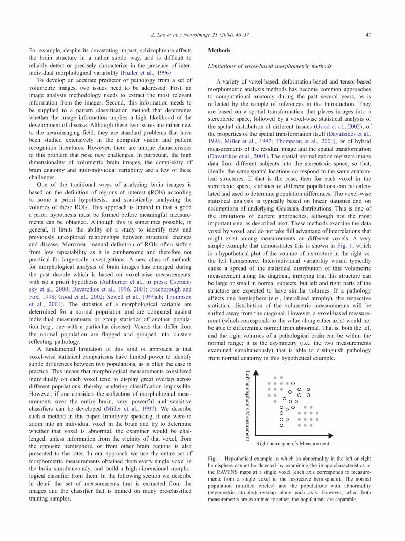
Fig. 1. Hypothetical example in which an abnormality in the left or right
hemisphere cannot be detected by examining the image characteristics or
the RAVENS maps at a single voxel (each axis corresponds to measure-
ments from a single voxel in the respective hemisphere). The normal
population (unfilled circles) and the populations with abnormality
(asymmetric atrophy) overlap along each axis. However, when both
measurements are examined together, the populations are separable.
Z. Lao et al. / NeuroImage 21 (2004) 46–57 47
For example, despite its devastating impact, schizophrenia affects
the brain structure in a rather subtle way, and is difficult to
reliably detect or precisely characterize in the presence of inter-
individual morphological variability (Haller et al., 1996).
To develop an accurate predictor of pathology from a set of
volumetric images, two issues need to be addressed. First, an
image analysis methodology needs to extract the most relevant
information from the images. Second, this information needs to
be supplied to a pattern classification method that determines
whether the image information implies a high likelihood of the
development of disease. Although these two issues are rather new
to the neuroimaging field, they are standard problems that have
been studied extensively in the computer vision and pattern
recognition literatures. However, there are unique characteristics
to this problem that pose new challenges. In particular, the high
dimensionality of volumetric brain images, the complexity of
brain anatomy and inter-individual variability are a few of these
challenges.
One of the traditional ways of analyzing brain images is
based on the definition of regions of interest (ROIs) according
to some a priori hypothesis, and statistically analyzing the
volumes of these ROIs. This approach is limited in that a good
a priori hypothesis must be formed before meaningful measure-
ments can be obtained. Although this is sometimes possible, in
general, it limits the ability of a study to identify new and
previously unexplored relationships between structural changes
and disease. Moreover, manual definition of ROIs often suffers
from low repeatability as it is cumbersome and therefore not
practical for large-scale investigations. A new class of methods
for morphological analysis of brain images has emerged during
the past decade which is based on voxel-wise measurements,
with no a priori hypothesis (Ashburner et al., in press; Csernan-
sky et al., 2000; Davatzikos et al., 1996, 2001; Freeborough and
Fox, 1998; Good et al., 2002; Sowell et al., 1999a,b; Thompson
et al., 2001). The statistics of a morphological variable are
determined for a normal population and are compared against
individual measurements or group statistics of another popula-
tion (e.g., one with a particular disease). Voxels that differ from
the normal population are flagged and grouped into clusters
reflecting pathology.
A fundamental limitation of this kind of approach is that
voxel-wise statistical comparisons have limited power to identify
subtle differences between two populations, as is often the case in
practice. This means that morphological measurements considered
individually on each voxel tend to display great overlap across
different populations, thereby rendering classification impossible.
However, if one considers the collection of morphological meas-
urements over the entire brain, very powerful and sensitive
classifiers can be developed (Miller et al., 1997). We describe
such a method in this paper. Intuitively speaking, if one were to
zoom into an individual voxel in the brain and try to determine
whether that voxel is abnormal, the examiner would be chal-
lenged, unless information from the vicinity of that voxel, from
the opposite hemisphere, or from other brain regions is also
presented to the rater. In our approach we use the entire set of
morphometric measurements obtained from every single voxel in
the brain simultaneously, and build a high-dimensional morpho-
logical classifier from them. In the following section we describe
in detail the set of measurements that is extracted from the
images and the classifier that is trained on many pre-classified
training samples.
Methods
Limitations of voxel-based morphometric methods
A variety of voxel-based, deformation-based and tensor-based
morphometric analysis methods has become common approaches
to computational anatomy during the past several years, as is
reflected by the sample of references in the Introduction. They
are based on a spatial transformation that places images into a
stereotaxic space, followed by a voxel-wise statistical analysis of
the spatial distribution of different tissues (Good et al., 2002), of
the properties of the spatial transformation itself (Davatzikos et al.,
1996; Miller et al., 1997; Thompson et al., 2001), or of hybrid
measurements of the residual image and the spatial transformation
(Davatzikos et al., 2001). The spatial normalization registers image
data from different subjects into the stereotaxic space, so that,
ideally, the same spatial locations correspond to the same anatom-
ical structures. If that is the case, then for each voxel in the
stereotaxic space, statistics of different populations can be calcu-
lated and used to determine population differences. The voxel-wise
statistical analysis is typically based on linear statistics and on
assumptions of underlying Gaussian distributions. This is one of
the limitations of current approaches, although not the most
important one, as described next. These methods examine the data
voxel by voxel, and do not take full advantage of interrelations that
might exist among measurements on different voxels. A very
simple example that demonstrates this is shown in Fig. 1, which
is a hypothetical plot of the volume of a structure in the right vs.
the left hemisphere. Inter-individual variability would typically
cause a spread of the statistical distribution of this volumetric
measurement along the diagonal, implying that this structure can
be large or small in normal subjects, but left and right parts of the
structure are expected to have similar volumes. If a pathology
affects one hemisphere (e.g., lateralized atrophy), the respective
statistical distribution of the volumetric measurements will be
shifted away from the diagonal. However, a voxel-based measure-
ment (which corresponds to the value along either axis) would not
be able to differentiate normal from abnormal. That is, both the left
and the right volumes of a pathological brain can be within the
normal range; it is the asymmetry (i.e., the two measurements
examined simultaneously) that is able to distinguish pathology
from normal anatomy in this hypothetical example.
Z. Lao et al. / NeuroImage 21 (2004) 46–5748
Although this is a very simplistic example, it demonstrates that
voxel-wise statistics are fundamentally limited by the fact that
different populations are most likely to have significant statistical
overlap on individual voxels, which would make their differenti-
ation via a voxel-wise analysis impossible. The interrelations
among measurements on different voxels are very important in
separating two or more populations, and therefore in predicting
whether a particular individual has or is likely to develop brain
pathology. These interrelations among voxel-wise morphological
measurements can be examined by statistical methods operating on
the very high dimensional space formed by measurements from all
voxels together. Although linear multivariate methods have been
previously proposed in the literature (McIntosh et al., 1996), we
have found that nonlinear methods result into much better charac-
terization of population differences. Our approach is based on the
use of nonlinear support vector machines (SVM) (Burges, 1998),
which have been shown to be one of the most powerful machine
learning methods, in conjunction with the entire collection of
morphological measurements from all voxels. These measurements
are obtained via a shape transformation that warps an individual
brain image to a template, thus forming a morphological signature
of the individual brain. We briefly summarize this shape transfor-
mation next. Details can be found in Shen and Davatzikos (2002,
2003).
Shape transformation using HAMMER
In this paper, we adopt an approach called hierarchical attribute
matching mechanism for elastic registration (HAMMER), which
was published in detail by Shen and Davatzikos (2002) and briefly
summarized here. HAMMER addresses two of the limitations that
are common among high-dimensional shape transformation meth-
ods. First, similarity of image intensities does not necessarily imply
anatomical correspondence. For example, mapping a gray matter
(GM) point of the precentral gyrus to a gray matter point of the
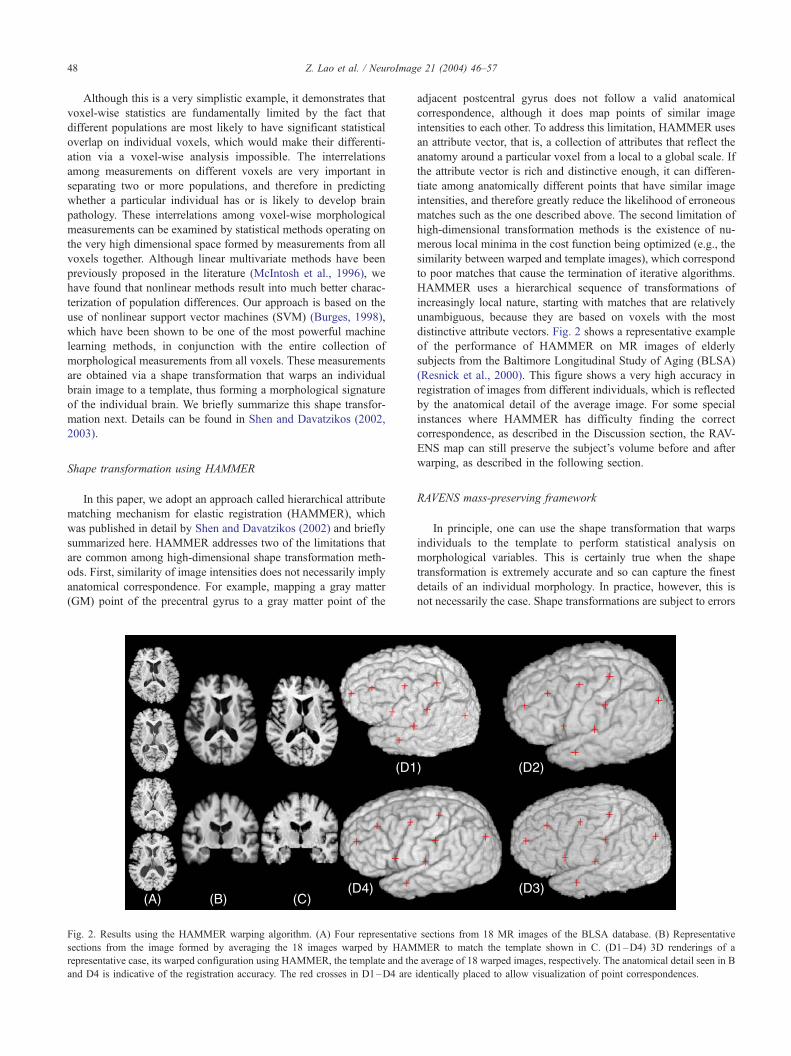
Fig. 2. Results using the HAMMER warping algorithm. (A) Four representative
sections from the image formed by averaging the 18 images warped by HAM
representative case, its warped configuration using HAMMER, the template and th
and D4 is indicative of the registration accuracy. The red crosses in D1–D4 are
adjacent postcentral gyrus does not follow a valid anatomical
correspondence, although it does map points of similar image
intensities to each other. To address this limitation, HAMMER uses
an attribute vector, that is, a collection of attributes that reflect the
anatomy around a particular voxel from a local to a global scale. If
the attribute vector is rich and distinctive enough, it can differen-
tiate among anatomically different points that have similar image
intensities, and therefore greatly reduce the likelihood of erroneous
matches such as the one described above. The second limitation of
high-dimensional transformation methods is the existence of nu-
merous local minima in the cost function being optimized (e.g., the
similarity between warped and template images), which correspond
to poor matches that cause the termination of iterative algorithms.
HAMMER uses a hierarchical sequence of transformations of
increasingly local nature, starting with matches that are relatively
unambiguous, because they are based on voxels with the most
distinctive attribute vectors. Fig. 2 shows a representative example
of the performance of HAMMER on MR images of elderly
subjects from the Baltimore Longitudinal Study of Aging (BLSA)
(Resnick et al., 2000). This figure shows a very high accuracy in
registration of images from different individuals, which is reflected
by the anatomical detail of the average image. For some special
instances where HAMMER has difficulty finding the correct
correspondence, as described in the Discussion section, the RAV-
ENS map can still preserve the subject’s volume before and after
warping, as described in the following section.
RAVENS mass-preserving framework
In principle, one can use the shape transformation that warps
individuals to the template to perform statistical analysis on
morphological variables. This is certainly true when the shape
transformation is extremely accurate and so can capture the finest
details of an individual morphology. In practice, however, this is
not necessarily the case. Shape transformations are subject to errors
sections from 18 MR images of the BLSA database. (B) Representative
MER to match the template shown in C. (D1–D4) 3D renderings of a
e average of 18 warped images, respectively. The anatomical detail seen in B
identically placed to allow visualization of point correspondences.
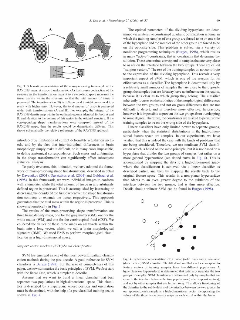
Fig. 3. Schematic representation of the mass-preserving framework of the
RAVENS maps. A shape transformation (A) that causes contraction of the
structure as the transformation maps it to a stereotaxic space increases the
tissue density within the structure, so that the total amount of tissue is
preserved. The transformation (B) is different, and it might correspond to a
result with higher error. However, the total amount of tissue is preserved
under both transformations (A and B). For example, the integral of the
RAVENS density map within the outlined region is identical for both A and
B, and identical to the volume of this region in the original structure. If the
corresponding shape transformations were compared instead of the
RAVENS maps, then the results would be dramatically different. This
shows schematically the relative robustness of the RAVENS approach.
Fig. 4. Schematic representation of a linear (solid line) and a nonlinear
(dotted curve) SVM classifier. The filled and unfilled circles correspond to
feature vectors of training samples from two different populations. A
hyperplane (or hypersurface) is determined that optimally separates the two
groups of samples. SVM classifiers are determined only by samples that are
close to the interface between the two populations (called support vectors),
and not by other samples that are further away. This allows fine-tuning of
the classifier to the subtle details of the interface between the two groups. In
our approach, each sample is a high-dimensional vector incorporating the
values of the three tissue density maps on each voxel within the brain.
Z. Lao et al. / NeuroImage 21 (2004) 46–57 49
introduced by limitations of current deformable registration meth-
ods, and by the fact that inter-individual differences in brain
morphology simply make it difficult, or in many cases impossible,
to define anatomical correspondence. Such errors and ambiguities
in the shape transformation can significantly affect subsequent
statistical analysis.
To partly overcome this limitation, we have adopted the frame-
work of mass-preserving shape transformations, described in detail
by Davatzikos (2001), Davatzikos et al. (2001) and Goldszal et al.
(1998). In this framework, we warp individual images to conform
with a template, while the total amount of tissue in any arbitrarily
defined region is preserved. This is accomplished by increasing or
decreasing the density of the tissue whenever the shape transforma-
tion contracts or expands the tissue, respectively. This approach
guarantees that the total mass within the region is preserved. This is
shown schematically in Fig. 3.
The results of the mass-preserving shape transformation are
three tissue density maps, one for the gray matter (GM), one for the
white matter (WM) and one for the cerebrospinal fluid (CSF). We
collected the values of these three maps on all voxels within the
brain into a long vector, which we call a brain morphological
signature (BMS). We used BMS to perform morphological classi-
fication in a high-dimensional space.
Support vector machine (SVM)-based classification
SVM has emerged as one of the most powerful pattern classifi-
cation methods during the past decade. A good reference for SVM
classifiers is Burges (1998). For the sake of completeness of this
paper, we now summarize the basic principles of SVM.We first start
with the linear case, which is simpler to describe.
Assume that we want to build a linear classifier that best
separates two populations in high-dimensional space. This classi-
fier is described by a hyperplane whose position and orientation
must be determined, with the help of a pre-classified training set, as
shown in Fig. 4.
The optimal parameters of the dividing hyperplane are deter-
mined via an iterative constrained quadratic optimization scheme, in
which the training samples of one group are forced to be on one side
of the hyperplane and the samples of the other group are forced to be
on the opposite side. This problem is solved via a variety of
nonlinear programming techniques (Burges, 1998), which results
in many ‘‘active’’ constraints, that is, constraints that determine the
solution. These constraints correspond to samples that are very close
to or are on the interface between the two groups. These are called
‘‘support vectors.’’ The rest of the training samples do not contribute
to the expression of the dividing hyperplane. This reveals a very
important aspect of SVM, which is one of the reasons for its
effectiveness as a classifier. The hyperplane is determined only by
a relatively small number of samples that are close to the opposite
group; the samples that are far away have no influence on the results,
because it is clear as to which group they belong. The classifier
inherently focuses on the subtleties of the morphological differences
between the two groups and not on gross differences that are not
difficult to detect, and is therefore more effective. In practice,
however, it is impossible to prevent the two groups from overlapping
to some degree. Therefore, the constraints are relaxed to permit some
training samples to be on the wrong side of the hyperplane.
Linear classifiers have only limited power to separate groups,
particularly when the statistical distributions in the high-dimen-
sional feature space are complex. In our experiments, we have
verified that this is indeed the case with the kinds of problems that
are being considered. Therefore, we use nonlinear SVM classifi-
cation which is based on the same principle, but it is not based on a
hyperplane that divides the two groups of samples, but rather on a
more general hypersurface (see dotted curve in Fig. 4). This is
accomplished by mapping the data to a high-dimensional space
where the classification is achieved via a linear classifier as
described earlier, and then by mapping the results back to the
original feature space. This results in a non-planar hypersurface
that adapts to an even greater degree to the subtleties of the
interface between the two groups, and is thus more effective.
Details about nonlinear SVM can be found in Burges (1998).
Z. Lao et al. / NeuroImage 21 (2004) 46–5750
Classification using the RAVENS maps
Our input to the SVM classifier is the morphological brain
signature, that is, the RAVENS maps of all tissues collectively.
Specifically, to perform morphological classification, we perform
the following steps:
1. RAVENS maps are smoothed via a 3D Gaussian filter, and the
resulting maps are downsampled by a factor of 4 in each
dimension. This reduces the number of variables that will be
used by the classifier by combining measurements from
neighboring voxels.
2. The resulting smoothed RAVENS values of the GM, WM and
CSF are concatenated into a long vector. Our segmentation
procedure of GM, WM and CSF employs a method based on
Markov random fields with inhomogeneity correction (Yan and
Karp, 1995). The vector is subsequently normalized to have unit
magnitude. Effectively, this normalizes for global brain size
differences. The resulting unit vector is the BMS. The
dimension of a typical RAVENS map is 256 � 256 � 124 in
voxels. The sizes of bounding boxes for WM and GM are
similar, around 180 � 140 � 123 in voxels while the size of
bounding box for VN is much smaller than that for WM and
GM, sometimes it can be negligible in calculating the dimension
of the feature vector. After downsampling by a factor of 4 in
each dimension, feature vector lengths for WM and GM are
48431 each. Concatenating the feature vectors for WM, GM and
VN, BMS ¼ ½WM GM VN� produces a brain morphological
signature, where WM; GM; VN are the feature vectors for
WM, GM and VN, respectively. Typically, a BMS has
dimensionality of order 105.
3. We train an SVM by providing the BMSs of many subjects. We
use a nonlinear SVM classifier by mapping the finite-length
brain signature data to a high-dimensional space via a Gaussian
kernel, as described by Burges (1998).
4. We apply the trained SVM classifier to a new subject. We
always test the SVM classifier on subjects not included in the
training set, as customary in classification methods.
Classification using ROIs obtained via warping a labeled atlas
Although the whole brain analysis achieved by including the
RAVENS values on every single voxel in the classification scheme,
in theory, is the most complete way of looking at the data, it
inevitably operates in a very high dimensional space (typically 104
to 105, after down-sampling the original RAVENS maps). It is
well-known that this makes a classifier vulnerable to noise,
particularly if only few training samples relative to the number
of voxels are available, which is the case when dealing with
medical images. For this reason, we also investigated alternative
ways of data representation, which are described in this and the
following subsections. In particular, we first used a region of
interest (ROI)-based approach by adopting a finely parcellated
brain image as a labeled atlas developed by Noor Kabani at the
Montreal Neurological Institute, including 101 ROIs. We then used
HAMMER to warp this atlas to individual subjects’ images,
thereby obtaining volumetric measurements of these ROIs for all
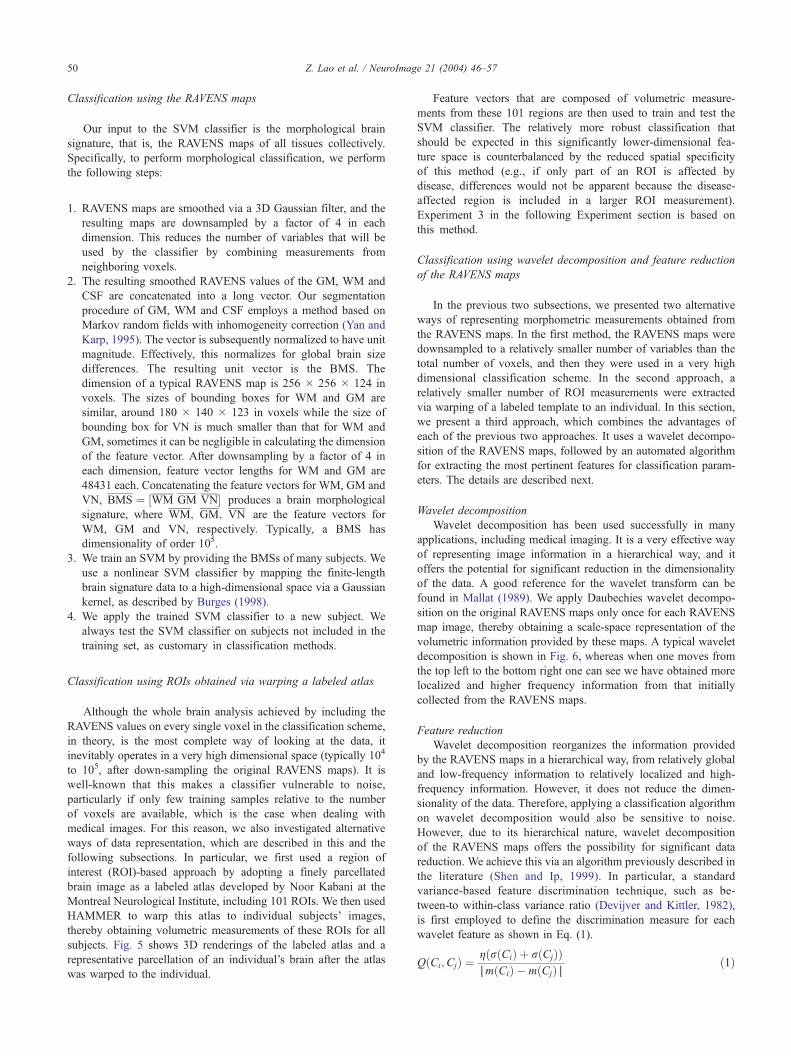
subjects. Fig. 5 shows 3D renderings of the labeled atlas and a
representative parcellation of an individual’s brain after the atlas
was warped to the individual.
Feature vectors that are composed of volumetric measure-
ments from these 101 regions are then used to train and test the
SVM classifier. The relatively more robust classification that
should be expected in this significantly lower-dimensional fea-
ture space is counterbalanced by the reduced spatial specificity
of this method (e.g., if only part of an ROI is affected by
disease, differences would not be apparent because the disease-
affected region is included in a larger ROI measurement).
Experiment 3 in the following Experiment section is based on
this method.
Classification using wavelet decomposition and feature reduction
of the RAVENS maps
In the previous two subsections, we presented two alternative
ways of representing morphometric measurements obtained from
the RAVENS maps. In the first method, the RAVENS maps were
downsampled to a relatively smaller number of variables than the
total number of voxels, and then they were used in a very high
dimensional classification scheme. In the second approach, a
relatively smaller number of ROI measurements were extracted
via warping of a labeled template to an individual. In this section,
we present a third approach, which combines the advantages of
each of the previous two approaches. It uses a wavelet decompo-
sition of the RAVENS maps, followed by an automated algorithm
for extracting the most pertinent features for classification param-
eters. The details are described next.
Wavelet decomposition
Wavelet decomposition has been used successfully in many
applications, including medical imaging. It is a very effective way
of representing image information in a hierarchical way, and it
offers the potential for significant reduction in the dimensionality
of the data. A good reference for the wavelet transform can be
found in Mallat (1989). We apply Daubechies wavelet decompo-
sition on the original RAVENS maps only once for each RAVENS
map image, thereby obtaining a scale-space representation of the
volumetric information provided by these maps. A typical wavelet
decomposition is shown in Fig. 6, whereas when one moves from
the top left to the bottom right one can see we have obtained more
localized and higher frequency information from that initially
collected from the RAVENS maps.
Feature reduction
Wavelet decomposition reorganizes the information provided
by the RAVENS maps in a hierarchical way, from relatively global
and low-frequency information to relatively localized and high-
frequency information. However, it does not reduce the dimen-
sionality of the data. Therefore, applying a classification algorithm
on wavelet decomposition would also be sensitive to noise.
However, due to its hierarchical nature, wavelet decomposition
of the RAVENS maps offers the possibility for significant data
reduction. We achieve this via an algorithm previously described in
the literature (Shen and Ip, 1999). In particular, a standard
variance-based feature discrimination technique, such as be-
tween-to within-class variance ratio (Devijver and Kittler, 1982),
is first employed to define the discrimination measure for each
wavelet feature as shown in Eq. (1).
QðCi;CjÞ ¼gðrðCiÞ þ rðCjÞÞAmðCiÞ � mðCjÞA
ð1Þ
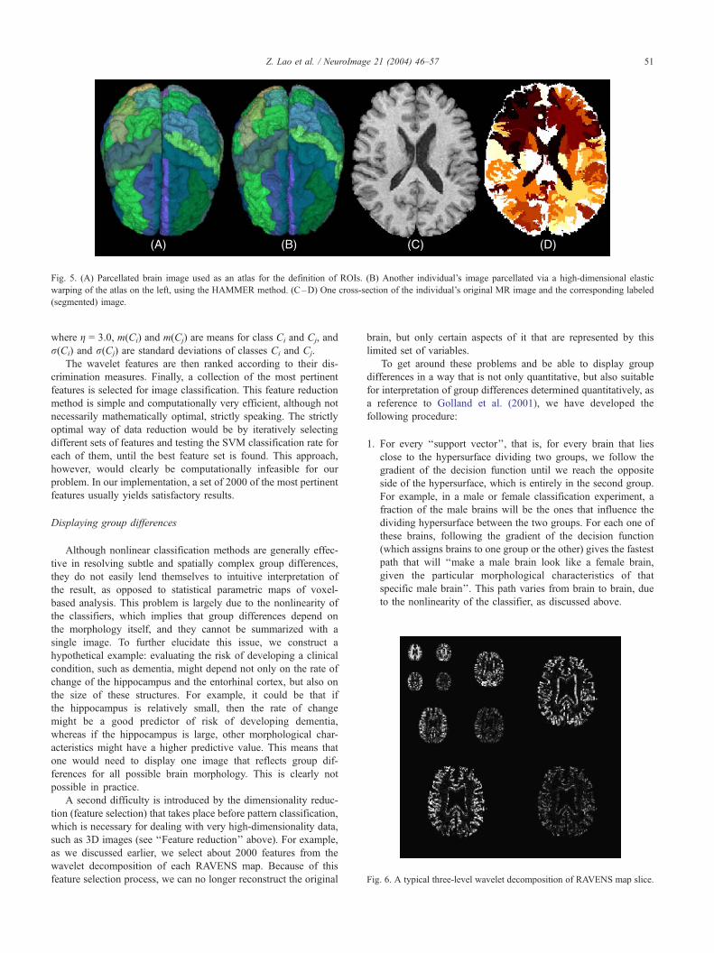
Fig. 6. A typical three-level wavelet decomposition of RAVENS map slice.
Fig. 5. (A) Parcellated brain image used as an atlas for the definition of ROIs. (B) Another individual’s image parcellated via a high-dimensional elastic
warping of the atlas on the left, using the HAMMER method. (C–D) One cross-section of the individual’s original MR image and the corresponding labeled
(segmented) image.
Z. Lao et al. / NeuroImage 21 (2004) 46–57 51
where g = 3.0, m(Ci) and m(Cj) are means for class Ci and Cj, and
r(Ci) and r(Cj) are standard deviations of classes Ci and Cj.
The wavelet features are then ranked according to their dis-
crimination measures. Finally, a collection of the most pertinent
features is selected for image classification. This feature reduction
method is simple and computationally very efficient, although not
necessarily mathematically optimal, strictly speaking. The strictly
optimal way of data reduction would be by iteratively selecting
different sets of features and testing the SVM classification rate for
each of them, until the best feature set is found. This approach,
however, would clearly be computationally infeasible for our
problem. In our implementation, a set of 2000 of the most pertinent
features usually yields satisfactory results.
Displaying group differences
Although nonlinear classification methods are generally effec-
tive in resolving subtle and spatially complex group differences,
they do not easily lend themselves to intuitive interpretation of
the result, as opposed to statistical parametric maps of voxel-
based analysis. This problem is largely due to the nonlinearity of
the classifiers, which implies that group differences depend on
the morphology itself, and they cannot be summarized with a
single image. To further elucidate this issue, we construct a
hypothetical example: evaluating the risk of developing a clinical
condition, such as dementia, might depend not only on the rate of
change of the hippocampus and the entorhinal cortex, but also on
the size of these structures. For example, it could be that if
the hippocampus is relatively small, then the rate of change
might be a good predictor of risk of developing dementia,
whereas if the hippocampus is large, other morphological char-
acteristics might have a higher predictive value. This means that
one would need to display one image that reflects group dif-
ferences for all possible brain morphology. This is clearly not
possible in practice.
A second difficulty is introduced by the dimensionality reduc-
tion (feature selection) that takes place before pattern classification,
which is necessary for dealing with very high-dimensionality data,
such as 3D images (see ‘‘Feature reduction’’ above). For example,
as we discussed earlier, we select about 2000 features from the
wavelet decomposition of each RAVENS map. Because of this
feature selection process, we can no longer reconstruct the original
brain, but only certain aspects of it that are represented by this
limited set of variables.
To get around these problems and be able to display group
differences in a way that is not only quantitative, but also suitable
for interpretation of group differences determined quantitatively, as
a reference to Golland et al. (2001), we have developed the
following procedure:
1. For every ‘‘support vector’’, that is, for every brain that lies
close to the hypersurface dividing two groups, we follow the
gradient of the decision function until we reach the opposite
side of the hypersurface, which is entirely in the second group.
For example, in a male or female classification experiment, a
fraction of the male brains will be the ones that influence the
dividing hypersurface between the two groups. For each one of
these brains, following the gradient of the decision function
(which assigns brains to one group or the other) gives the fastest
path that will ‘‘make a male brain look like a female brain,
given the particular morphological characteristics of that
specific male brain’’. This path varies from brain to brain, due
to the nonlinearity of the classifier, as discussed above.
Z. Lao et al. / NeuroImage 21 (2004) 46–5752
2. From the paths determined in Step 1, apply the inverse wavelet
transform and construct images that highlight group differences
for each of these brains.
3. Average these group difference images for all support vectors so
that a single map can be constructed.
4. Find all local maxima of the clusters that are formed in Step 3;
these local maxima show the regions which are most
informative in terms of resolving group differences.
5. Overlay these local maxima on the brain image used as template
for anatomical reference purposes.
Of course, Step 3 could be omitted. However, in that case, one
would need to show one difference map for every single brain.
Experiments
In this section we provide experiments that demonstrate the
performance of our approach using magnetic resonance images of
healthy older adults who are participants in the Baltimore Longi-
tudinal Study of Aging (BLSA). These individuals range in age
from 56 to 85 and undergo yearly structural scans, among other
evaluations, using a standard SPGR protocol. Details about the
subjects and the image acquisition parameters can be found in
Resnick et al. (2000).
In summary, there are three classification schemes as described
in (1) ‘‘Classification using the RAVENS maps’’; (2) ‘‘Classifica-
tion using ROIs obtained via warping a labeled atlas’’; and (3)
‘‘Classification using wavelet decomposition and feature reduction
of the RAVENS maps’’, respectively. The first scheme used down-
sampled original RAVENS maps as features for classification; the
second scheme used ROI-based features for classification and the
third scheme used wavelet transformed RAVENS maps combined
with a feature selection scheme to select a set of most prominent
wavelet coefficients as features for classification. Experiment 2
used the first scheme; Experiment 3 used the second scheme;
Experiments 1, 4, 5 and 6 used the third scheme. Experiment 7 is
based on the result of the third classification scheme, but it also
used techniques described in ‘‘Display group differences’’.
Experiment 1: response in the absence of any effect
To test that there is no bias in our classifier, we tested the
hypothesis that under no effect, the response should be detection of
no group differences. Accordingly, we performed a random per-
mutation experiment. Specifically, we randomly assigned the 153
individual subjects to two different groups. Using the leave-one-
out method, we then tested our method. We repeated this exper-
iment using 20 random permutations. The average classification
rate was 48%, which agrees very well with our expectation that this
experiment should lead to a nearly ‘‘coin-toss’’ success rate (which
would be 50%).
Simulated atrophy
Weperformed two experiments (Experiment 2 andExperiment 3)
in which we simulated morphological effects in two different ways
on images from older adults of the BLSA study, thereby generating
a second set of the same number of images displaying systematic
morphological differences in certain parts of the brain. Our goal
was to test whether our classification method would correctly
discriminate between these two groups, providing results that
revealed brain differences in a systematic way.
Experiment 2
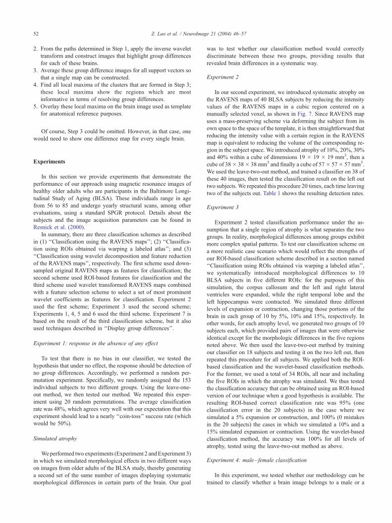
In our second experiment, we introduced systematic atrophy on
the RAVENS maps of 40 BLSA subjects by reducing the intensity
values of the RAVENS maps in a cubic region centered on a
manually selected voxel, as shown in Fig. 7. Since RAVENS map
uses a mass-preserving scheme via deforming the subject from its
own space to the space of the template, it is then straightforward that
reducing the intensity value with a certain region in the RAVENS
map is equivalent to reducing the volume of the corresponding re-
gion in the subject space. We introduced atrophy of 10%, 20%, 30%
and 40% within a cube of dimensions 19 � 19 � 19 mm3, then a
cube of 38� 38� 38 mm3 and finally a cube of 57� 57� 57 mm3.
We used the leave-two-out method, and trained a classifier on 38 of
these 40 images, then tested the classification result on the left out
two subjects. We repeated this procedure 20 times, each time leaving
two of the subjects out. Table 1 shows the resulting detection rates.
Experiment 3
Experiment 2 tested classification performance under the as-
sumption that a single region of atrophy is what separates the two
groups. In reality, morphological differences among groups exhibit
more complex spatial patterns. To test our classification scheme on
a more realistic case scenario which would reflect the strengths of
our ROI-based classification scheme described in a section named
‘‘Classification using ROIs obtained via warping a labeled atlas’’,
we systematically introduced morphological differences to 10
BLSA subjects in five different ROIs: for the purposes of this
simulation, the corpus callosum and the left and right lateral
ventricles were expanded, while the right temporal lobe and the
left hippocampus were contracted. We simulated three different
levels of expansion or contraction, changing those portions of the
brain in each group of 10 by 5%, 10% and 15%, respectively. In
other words, for each atrophy level, we generated two groups of 10
subjects each, which provided pairs of images that were otherwise
identical except for the morphologic differences in the five regions
noted above. We then used the leave-two-out method by training
our classifier on 18 subjects and testing it on the two left out, then
repeated this procedure for all subjects. We applied both the ROI-
based classification and the wavelet-based classification methods.
For the former, we used a total of 34 ROIs, all near and including
the five ROIs in which the atrophy was simulated. We thus tested
the classification accuracy that can be obtained using an ROI-based
version of our technique when a good hypothesis is available. The
resulting ROI-based correct classification rate was 95% (one
classification error in the 20 subjects) in the case where we
simulated a 5% expansion or construction, and 100% (0 mistakes
in the 20 subjects) the cases in which we simulated a 10% and a
15% simulated expansion or contraction. Using the wavelet-based
classification method, the accuracy was 100% for all levels of
atrophy, tested using the leave-two-out method as above.
Experiment 4: male–female classification
In this experiment, we tested whether our methodology can be
trained to classify whether a brain image belongs to a male or a
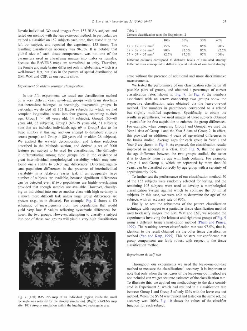
Table 1
Correct classification rates for Experiment 2
10% 20% 30% 40%
19 � 19 � 19 mm3 75% 80% 85% 90%
38 � 38 � 38 mm3 80% 82.5% 85% 92.5%
57 � 57 � 57 mm3 82.5% 87.5% 95% 100%
Different columns correspond to different levels of simulated atrophy.
Different rows correspond to different spatial extents of simulated atrophy.
Z. Lao et al. / NeuroImage 21 (2004) 46–57 53
female individual. We used images from 153 BLSA subjects and
tested our method with the leave-one-out method. In particular, we
trained a classifier on 152 subjects each time, then tested it on the
left out subject, and repeated the experiment 153 times. The
resulting classification accuracy was 96.7%. It is notable that
global size of each tissue compartment was not one of the
parameters used in classifying images into males or females,
because the RAVENS maps are normalized to unity. Therefore,
the female and male brains differ not only in global size, which is a
well-known fact, but also in the pattern of spatial distribution of
GM, WM and CSF, as our results show.
Experiment 5: older–younger classification
In our fifth experiment, we tested our classification method
on a very difficult case, involving groups with brain structures
that heretofore belonged to seemingly inseparable groups. In
particular, we divided all 153 BLSA subjects for which we had
complete longitudinal scans into four groups, according to their
age: Group1 ( < 60 years old, 14 subjects), Group2 (60–68
years old, 62 subjects), Group3 (69–79 years old, 51 subjects;
note that we included individuals age 69 in Group3 due to the
large number at this age and our attempt to distribute subjects
across groups) and Group 4 (80 years old or older, 26 subjects).
We applied the wavelet decomposition and feature reduction
described in the Methods section, and derived a set of 2000
features per subject to be used for classification. The difficulty
in differentiating among these groups lies in the existence of
great interindividual morphological variability, which may con-
found one’s ability to detect age differences. Detecting signifi-
cant population differences in the presence of interindividual
variability is a relatively easier task if an adequately large
number of subjects are available, because significant differences
can be detected even if two populations are highly overlapping
provided that enough samples are available. However, classify-
ing an individual into one or another class with high certainty is
a much more difficult task unless large group differences are
present (e.g., as in disease). For example, Fig. 8 shows a 1D
schematic of measurements from two populations that would
yield very low P values reflecting systematic differences be-
tween the two groups. However, attempting to classify a subject
into one of these two groups will yield a very high classification
Fig. 7. (Left) RAVENS map of an individual (region inside the small
rectangle was selected for the atrophy simulation). (Right) RAVENS map
after 10% atrophy simulation within the highlighted rectangular area.
error without the presence of additional and more discriminative
measurements.
We tested the performance of our classification scheme on all
possible pairs of groups, and obtained a percentage of correct
classification rates, shown in Fig. 9. In Fig. 9, the numbers
associated with an arrow connecting two groups show the
respective classification rates obtained via the leave-one-out
method. The numbers in parentheses correspond to a related
but slightly modified experiment. Specifically, to obtain the
results in parentheses, we used images of these subjects obtained
4 years after the first acquisition to enhance the group differences.
For example, when comparing Group1 and Group2, we used the
Year 1 data of Group 1 and the Year 5 data of Group 2. In effect,
this provided an additional 4 years of age-related differences to
the brains studied. Average ages for each group in Year 1 and
Year 5 are shown in Fig. 9. As expected, the classification results
improved in general: it is clear, from Fig. 9, that the greater
the age difference between the two groups studied, the easier
it is to classify them by age with high certainty. For example,
Group 1 and Group 4, which are separated by more than 20
years, can be classified correctly by age group with a certainty of
approximately 97%.
To further test the performance of our classification method, 50
of the 153 subjects were randomly selected for testing, and the
remaining 103 subjects were used to develop a morphological
classification system against which to compare the 50 initial
subjects. In this case, we were able to determine the age of the
subjects with an accuracy rate of 90%.
Finally, to test the robustness of the pattern classification
technique with respect to a particular tissue classification method
used to classify images into GM, WM and CSF, we repeated the
experiments involving the leftmost and rightmost groups of Fig. 9
using a different tissue classification method (Pham and Prince,
1999). The resulting correct classification rate was 97.5%, that is,
identical to the result obtained via the other tissue classification
method (Yan and Karp, 1995). This bolsters our confidence that
group comparisons are fairly robust with respect to the tissue
classification method.
Experiment 6: self test
Throughout our experiments we used the leave-one-out-like
method to measure the classifications’ accuracy. It is important to
note that only when the test cases of the leave-one-out method are
not included can we get accurate estimates of the classification rate.
To illustrate this, we applied our methodology to the data consid-
ered in Experiment 5, which had resulted in a classification rate
between Group 1 and Group 3 of only 83% with the leave-one-out
method. When the SVM was trained and tested on the same set, the
accuracy was 100%. Fig. 10 shows the values of the classifier
function for each subject.
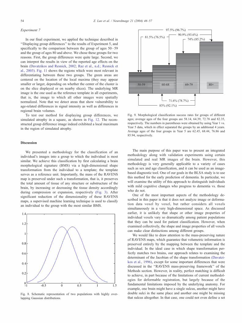
Fig. 9. Morphological classification success rates for groups of different
ages; average ages of the four groups are 58.14, 64.39, 72.78 and 82.35,
respectively. The numbers in parentheses were obtained by using Year 1 vs.
Year 5 data, which in effect separated the groups by an additional 4 years.
oImage 21 (2004) 46–57
Experiment 7
In our final experiment, we applied the technique described in
‘‘Displaying group differences’’ to the results of Experiment 5, and
specifically to the comparison between the group of ages 50–59
and the group of ages 80 and above. We chose these groups for two
reasons. First, the group differences were quite large. Second, we
can interpret the results in view of the reported age effects on the
brain (Davatzikos and Resnick, 2002; Raz et al., n.d.; Resnick et
al., 2003). Fig. 11 shows the regions which were most relevant in
differentiating between these two groups. The green areas are
centered on the location of the local maxima (they may appear
smaller or larger, depending on whether the center of the cluster is
on the slice displayed or on nearby slices). The underlying MR
image is the one used as the reference template in all experiments,
that is, the image to which all other images were spatially
normalized. Note that we detect areas that show vulnerability to
age-related differences in signal intensity as well as differences in
regional brain volumes.
To test our method for displaying group differences, we
simulated atrophy in a square, as shown in Fig. 12. The recon-
structed group difference image indeed exhibited a local maximum
in the region of simulated atrophy.
Z. Lao et al. / Neur54
Average ages of the four groups in Year 5 are 62.45, 68.44, 76.86 and
85.94, respectively.
Discussion
We presented a methodology for the classification of an
individual’s images into a group to which the individual is most
similar. We achieve this classification by first calculating a brain
morphological signature (BMS) via a high-dimensional shape
transformation from the individual to a template; the template
serves as a reference unit. Importantly, the mass of the RAVENS
map is preserved under such a transformation, that is, it preserves
the total amount of tissue of any structure or substructure of the
brain, by increasing or decreasing the tissue density accordingly
during compression or expansion, respectively (Fig. 3). After
significant reduction of the dimensionality of these RAVENS
maps, a supervised machine learning technique is used to classify
an individual to the group with the most similar BMS.
Fig. 8. Schematic representation of two populations with highly over-
lapping Gaussian distributions.
The main purpose of this paper was to present an integrated
methodology along with validation experiments using certain
simulated and real MR images of the brain. However, this
methodology is very generally applicable to a variety of cases
such as sex and age classification, and it can be used as an image-
based diagnostic tool. One of our goals in the BLSA study is to use
this method for the early prediction of dementia. In particular, we
will examine the utility of this approach to distinguish individuals
with mild cognitive changes who progress to dementia vs. those
who do not.
One of the most important aspects of the methodology de-
scribed in this paper is that it does not analyze image or deforma-
tion data voxel by voxel, but rather considers all voxels
simultaneously in a very high-dimensional space. As discussed
earlier, it is unlikely that shape or other image properties of
individual voxels vary so dramatically among patient populations
that they can be used for patient classification. However, when
examined collectively, the shape and image properties of all voxels
can make clear distinctions among different groups.
We would like to draw attention to the mass-preserving nature
of RAVENS maps, which guarantee that volumetric information is
preserved entirely by the mapping between the template and the
individual. In the ideal case in which shape transformation per-
fectly matches two brains, our approach relates to examining the
determinant of the Jacobian of the shape transformation (Davatzi-
kos et al., 1996), except for some important differences that were
discussed in the ‘‘RAVENS mass-preserving framework’’ of the
Methods section. However, in reality, perfect matching is difficult
to achieve, in part because of the limitations of current methodol-
ogies for deformable registration, but largely because of the
fundamental limitations imposed by the underlying anatomy. For
example, one brain might have a single sulcus, another might have
double sulci in the same place and another one might be missing
that sulcus altogether. In that case, one could not even define a set
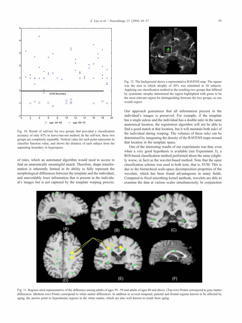
Fig. 10. Result of self-test for two groups that provided a classification
accuracy of only 83% in leave-one-out method. In the self-test, these two
groups are completely separable. Vertical value for each point represents its
classifier function value, and shows the distance of each subject from the
separating boundary in hyperspace.
Fig. 12. The background shows a representative RAVENS map. The square
was the area in which atrophy of 20% was simulated in 20 subjects.
Applying our classification method to the resulting two groups that differed
by systematic atrophy determined the region highlighted with green to be
the most relevant region for distinguishing between the two groups, as one
would expect.
Z. Lao et al. / NeuroImage 21 (2004) 46–57 55
of rules, which an automated algorithm would need to access to
find an anatomically meaningful match. Therefore, shape transfor-
mation is inherently limited in its ability to fully represent the
morphological differences between the template and the individual,
and unavoidably loses information that is present in the individu-
al’s images but is not captured by the template warping process.
Fig. 11. Regions most representative of the difference among adults of ages 50–59
differences. (Bottom row) Points correspond to white matter differences. In additi
aging, the arrows point to hypointense regions in the white matter, which are als
Our approach guarantees that all information present in the
individual’s images is preserved. For example, if the template
has a single sulcus and the individual has a double sulci in the same
anatomical location, the registration algorithm will not be able to
find a good match at that location, but it will maintain both sulci of
the individual during warping. The volumes of these sulci can be
determined by integrating the density of the RAVENS maps around
that location in the template space.
One of the interesting results of our experiments was that, even
when a very good hypothesis is available (see Experiment 3), a
ROI-based classification method performed about the same (slight-
ly worse, in fact) as the wavelet-based method. Note that the same
classification scheme was used in both tests, that is, SVM. This is
due to the hierarchical scale-space decomposition properties of the
wavelets, which has been found advantageous in many fields.
Compared to fixed smoothing kernel methods, wavelets are able to
examine the data at various scales simultaneously. In conjunction
and adults of ages 80 and above. (Top row) Points correspond to gray matter
on to several temporal, parietal and frontal regions known to be affected by
o well known to result from aging.
Z. Lao et al. / NeuroImage 21 (2004) 46–5756
with the pattern classification step, this presumably allows the
classifier to find the dimension along, or equivalently the scale at,
which best differentiation between the two groups can be achieved.
Notably, this is achieved without increase of the dimensionality of
the search space, as would be the case when smoothing the data
with Gaussian kernels of various widths.
Pattern classification is particularly suitable as a diagnostic tool.
However, displaying group differences determined by the classifier
in an intuitive way that allows further interpretation of the results is
a difficult issue, as discussed in Displaying group differences. We
presented an approach to overcome some of the limitations
inherent in displaying population differences, which is based on
determining the local maxima of clusters that have the most
relevant information for distinguishing two groups. Improvements
of this basic technique are possible. Specifically, in constructing
difference images obtained by following the gradient of the
decision function, we assumed that all wavelet coefficients not
included in our feature vector, that is, all coefficients that were
dropped during the feature reduction step, were the same in the two
groups. This is a reasonable assumption, because these variables
are never used in classification, therefore their values are irrelevant
for classification. However, wavelet coefficients across different
scales are correlated, because they are linked, to some extent, to the
same spatial location. Taking these correlations into account might
lead to better estimates of the variables not used in our feature set
but used for reconstruction of the difference among groups via the
inverse wavelet transform.
Acknowledgments
The datasets used in the experiments were obtained under the
Baltimore Longitudinal Study of Aging (BLSA). This work was
supported in part by NIH grant R01 AG14971 and by NIH contract
AG-93-07.
References
Arenillas, J.F., Rovira, A., Molina, C.A., Grive, E., Montaner, J., et al.,
2002. Prediction of early neurological deterioration using diffusion- and
perfusion-weighted imaging in hyperacute middle cerebral artery ische-
mic stroke. Stroke 33, 2197–2205.
Ashburner, J., Csernansky, J.G., Davatzikos, C., Fox, N.C., et al., 2003.
Computer-assisted imaging to assess brain structure in healthy and dis-
eased brains. Lancet (Neurology) 2, 79–88.
Bobinski, M., de Leon, M.J., Convit, A., De Santi, S., et al., 1999. MRI
of entorhinal cortex in mild Alzheimer’s disease. Lancet 353 (9146),
38–40.
Braak, H., Braak, E., Bohl, J., Bratzke, H., 1998. Evolution of Alz-
heimer’s disease related cortical lesions. J. Neural Transm., Suppl.
54, 97–106.
Brown, W.E., Eliez, S., Menon, V., et al., 2001. Preliminary evidence of
widespread morphological variations of the brain in Dyslexia. Neurol-
ogy 56 (6), 781–783 (Mar. 27).
Burges, C.J.C., 1998. A tutorial on support vector machines for pattern
recognition. Data Min. Knowl. Discov. 2 (2), 121–167.
Csernansky, J.G., Wang, L., Joshi, S., Miller, J.P., et al., 2000. Early DAT is
distinguished from aging by high-dimensional mapping of the hippo-
campus. Neurology 55, 1636–1643.
Davatzikos, C., 2001. Measuring biological shape using geometry-based
shape transformations. J. Image Vis. Comp. 19, 63–74.
Davatizkos, C., Resnick, S.M., 2002. Degenerative age changes in white
matter connectivity visualized in vivo using magnetic resonance imag-
ing. Cereb. Cortex 12 (7), 767–771.
Davatzikos, C., Vaillant, M., Resnick, S., Prince, J.L., et al., 1996. A
computerized approach for morphological analysis of the corpus callos-
um. J. Comput. Assist. Tomogr. 20, 88–97.
Davatzikos, C., Genc, A., Xu, D., Resnick, S.M., 2001. Voxel-based
morphometry using the RAVENS maps: methods and validation using
simulated longitudinal atrophy. NeuroImage 14, 1361–1369.
DeLeon, M.J., George, A.E., Golomb, J., Tarshish, C., et al., 1991. Fre-
quency of hippocampal formation atrophy in normal aging and Alz-
heimer’s Disease. Neurobiol. Aging 18, 1–11.
deToledo-Morrell, L., Sullivan, M.P., Morrell, F., Wilson, R.S., et al., 1997.
Alzheimer’s disease: in vivo detection of differential vulnerability of
brain regions. Neurobiol. Aging 18, 463–538.
Devijver, P.A., Kittler, J., 1982. Pattern Recognition: A Statistical Ap-
proach. Prentice-Hall, Englewood Cliffs, NJ.
Freeborough, P.A., Fox, N.C., 1998. Modeling brain deformations in Alz-
heimer’s disease by fluid registration of serial 3D MR images. J. Comp.
Assist. Tomogr. 22, 838–843.
Giedd, J.N., Blumenthal, J., Jeffries, N.O., Castellanos, F.X., Liu, H., Zij-
denbos, A., Paus, T., Evans, A.C., Rapoport, J.L., 1999. Brain develop-
ment during childhood and adolescence: a longitudinal MRI study. Nat.
Neurosci. 2, 861–863.
Goldszal, A.F., Davatzikos, C., Pham, D., Yan, M., et al., 1998. An image
processing protocol for the analysis of MR images from an elderly
population. J. Comp. Assist. Tomogr. 22 (5), 827–837.
Golland, P., Grimson, W.E.L., Shenton, M.E., Kikinis, R., 2001. Deforma-
tion analysis for shape based classification. In Proc. IPMI’LNCS 2082,
517–530.
Golomb, J., deLeon, M.J., Kluger, A., George, A.E., et al., 1993. Hippo-
campal atrophy in normal aging: an association with recent memory
impairment. Arch. Neurol. 50 (9), 967–973.
Gomez-Isla, T., Price, J.L., McKeel, D.W.J., Morris, J.C., et al., 1996.
Profound loss of layer II entorhinal cortex neurons occurs in very mild
Alzheimer’s disease. J. Neurosci. 16, 4491–4500.
Good, C.D., Scahill, R.I., Fox, N.C., Ashburner, J., et al., 2002. Automatic
differentiation of anatomical patterns in the human brain: validation
with studies of degenerative dementias. NeuroImage 17 (1), 29–46.
Haller, J.W., Christensen, G.E., et al., 1996. Hippocampal MR imaging
morphometry by means of general pattern matching. Radiology 199,
787–791.
Hyman, B.T., 1997. The neuropathological diagnosis of Alzheimer’s
disease: clinical –pathological studies. Neurobiol. Aging 18 (S4),
S27–S32.
Hyman, B.T., Hoesen, G.W.V., Damasio, A.R., Barnes, C.L., 1984. Alz-
heimer’s disease: cell-specific pathology isolates the hippocampal for-
mation. Science 225, 1168–1170.
Jack, J.C.R., Twomey, C.K., Zinsmeister, A., Sharbrough, F.W., et al.,
1989. Anterior temporal lobes and hippocampal formations: normative
volumetric measurements from MR images in young adults. Radiology
172, 549–554.
Jobst, K.A., Smith, A.D., Szatmari, M., Esiri, M.M., et al., 1994. Rapidly
progressing atrophy of medial temporal lobe in Alzheimer’s disease.
Lancet 343, 829–830.
Killiany, R.J., Gomez-Isla, T., et al., 2000. Use of structural magnetic
resonance imaging to predict who will get Alzheimer’s disease. Ann.
Neurol. 47 (4), 430–439.
Lamar, M., Resnick, S.M., Zonderman, A.B., 2003. Longitudinal changes
in verbal memory in older adults: distinguishing the effects of age from
repeat testing. Neurology 60 (1), 82–86.
Mallat, S.G., 1989. A theory for multiresolution signal decomposition: the
wavelet representation. IEEE Trans. Pattern Anal. Mach. Intell. 11 (7),
674–693.
McIntosh, A.R., Bookstein, F.L., Haxby, J.V., Grady, C.L., 1996. Spatial
pattern analysis of functional brain images using partial least squares.
NeuroImage 3, 143–157.
Z. Lao et al. / NeuroImage 21 (2004) 46–57 57
Miller, M., Banerjee, A., Christensen, G., Joshi, S., et al., 1997. Stat-
istical methods in computational anatomy. Stat. Methods Med. Res.
6, 267–299.
Morris, J.C., Heyman, A., Mohs, R.C., Hughes, J.P., et al., 1989. The
consortium to establish a registry for Alzheimer’s disease (CERAD).
Part I. Clinical and neuropsychological assessment of Alzheimer’s dis-
ease. Neurology 39 (9), 1159–1165.
Pham, D.L., Prince, J.L., 1999. An adaptive fuzzy C-means algorithm for
image segmentation in the presence of intensity inhomogeneities. Pat-
tern Recogn. Lett. 20 (1), 57–68.
Raz, N., Dixon, F.M., Head, D.P., Dupuis, J.H., Acker, J.D., 1998. Neuro-
anatomical correlates of cognitive aging: evidence from structural MRI.
Neuropsychology 12, 95–106.
Resnick, S.M., Goldszal, A.F., Davatzikos, C., Golski, S., et al., 2000. One-
year age changes in MRI brain volumes in older adults. Cereb. Cortex
10, 464–472.
Resnick, S.M., Pham, D.L., Kraut, M.A., Zonderman, A.B., Davatzikos,
C., 2003. Longitudinal magnetic resonance imaging studies of older
adults: a shrinking brain. J. Neurosci. 23 (8), 3295–3301.
Shen, D., Davatzikos, C., 2002. HAMMER: hierarchical attribute matching
mechanism for elastic registration. IEEE Trans. Med. Imag. 21 (11),
1421–1439.
Shen, D.G., Davatzikos, C., 2003. Very high resolution morphometry using
mass-preserving deformations and HAMMER elastic registration. Neu-
roImage 18 (1), 28–41.
Shen, D., Ip, H.H.S., 1999. Discriminative wavelet shape descriptors for
invariant recognition of 2-D patterns. Pattern Recogn. 32 (2), 151–165.
Shen, D., Lao, Z., Zeng, J., Herskovits, E.H., Fichtinger, G., Davatzikos,
C., 2001. ‘‘A Statistical Atlas of Prostate Cancer for Optimal Biopsy’’,
MICCAI2001, 416–424 (October).
Sowell, E.R., Thompson, P.M., Holmes, C.J., Batth, R., et al., 1999a.
Localizing age-related changes in brain structure between childhood
and adolescence using statistical parametric mapping. NeuroImage 9
(6 (Pt1)), 587–597.
Sowell, E.R., Thompson, P.M., Holmes, C.J., Jernigan, T.L., et al., 1999b.
In vivo evidence for post-adolescent brain maturation in front and stria-
tal regions. Nat. Neurosci. 2 (10), 859–861.
Sowell, E.R., Trauner, D.A., Gamst, A., Jernigan, T.L., 2002. Develop-
ment of cortical and subcortical brain structures in childhood and
adolescence: a structural MRI study’’. Dev. Med. Child Neurol. 44
(1), 4–16 (January).
Sullivan, E.V., Pfefferbaum, A., Adalsteinsson, E., Swan, G.E., et al., 2002.
Differential rates of regional brain change in callosal and ventricular
size: a 4-year longitudinal MRI study of elderly men. Cereb. Cortex 12
(4), 438–445.
Thompson, P.M., Mega, M.S., Woods, R.P., Zoumalan, C.I., et al., 2001.
Cortical change in Alzheimer’s disease detected with a disease-specific
population based Brain Atlas. Cereb. Cortex 11 (1), 1–16.
Visser, P.J., Verhey, F.R.J., Hofman, P.A., Scheltens, P., et al., 2002. Medial
temporal lobe atrophy predicts Alzheimer’s disease in patients with
minor cognitive impairment. J. Neurol. Neurosurg. Psychiatry 72 (4),
491–497.
Weiner, M., DeCarli, C., deLeon, M., Fox, N., Jack, C., Scheltens, P.,
Small, G., Katchatiruan, Z., Peterson, R., Thal, L., 2001. Neuroimaging
for detection, diagnosis and monitoring of Alzheimer’s disease and
other dementias: proceedings of the Alzheimer’s imaging consortium.
Neurobiol. Aging 22, 331–342.
Yan, M.X.H., Karp, J.S., 1995. An adaptive Bayesian approach to three-
dimensional MR image segmentation. Proc. of the Conf. on Inform.
Proc. in Med. Imag.