MORPHODYNAMICS OF SAND-BED RIVERS ENDING IN DELTAS

1

Contribution from the National Center for Earth-surface Dynamics

for the Short Course

Environmental Fluid Mechanics: Theory, Experiments and Applications

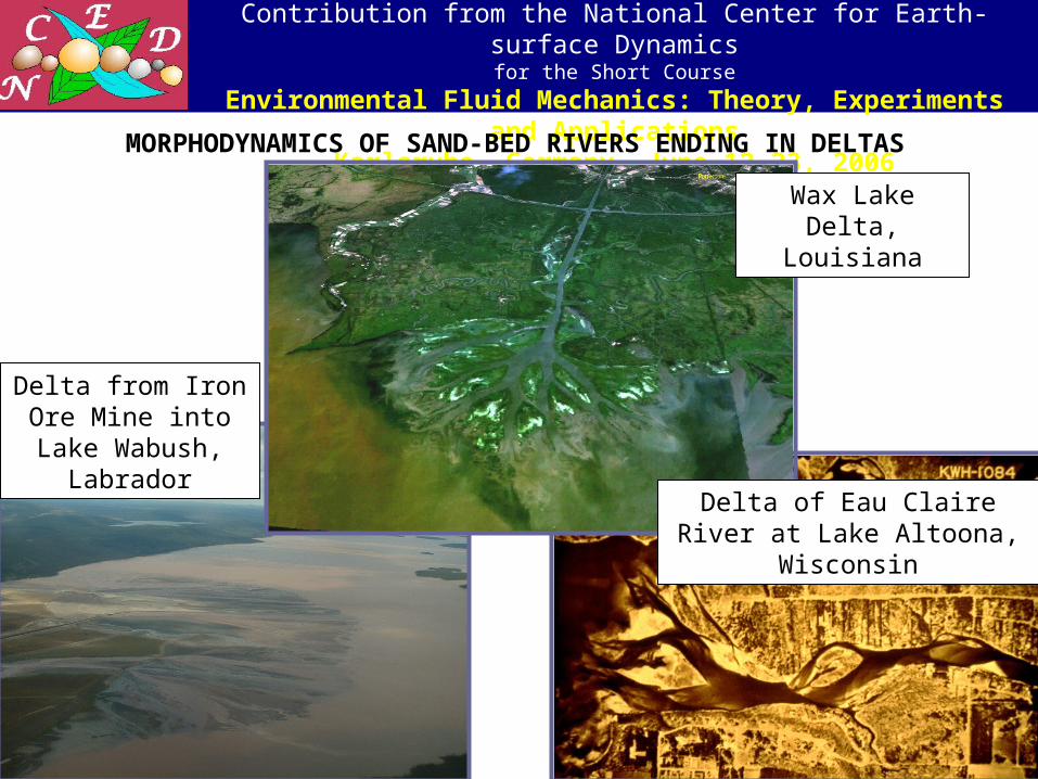
Karlsruhe, Germany, June 12-23, 2006MORPHODYNAMICS OF SAND-BED RIVERS ENDING IN DELTAS

Wax Lake Delta, Louisiana

Delta of Eau Claire River at Lake Altoona, Wisconsin

Delta from Iron Ore Mine into Lake Wabush,

Labrador

2




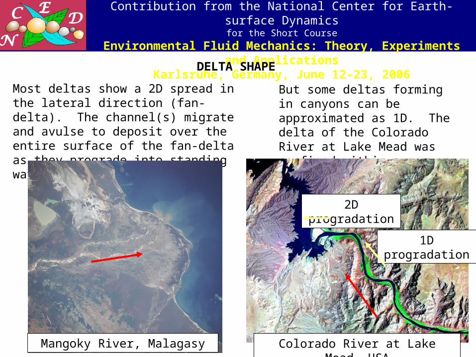
Karlsruhe, Germany, June 12-23, 2006DELTA SHAPE

Most deltas show a 2D spread in the lateral direction (fan-delta). The channel(s) migrate and avulse to deposit over the entire surface of the fan-delta as they prograde into standing water.

Mangoky River, Malagasy

But some deltas forming in canyons can be approximated as 1D. The delta of the Colorado River at Lake Mead was confined within a canyon until recently.

Colorado River at Lake Mead, USA

1D progradation

2D progradation

3




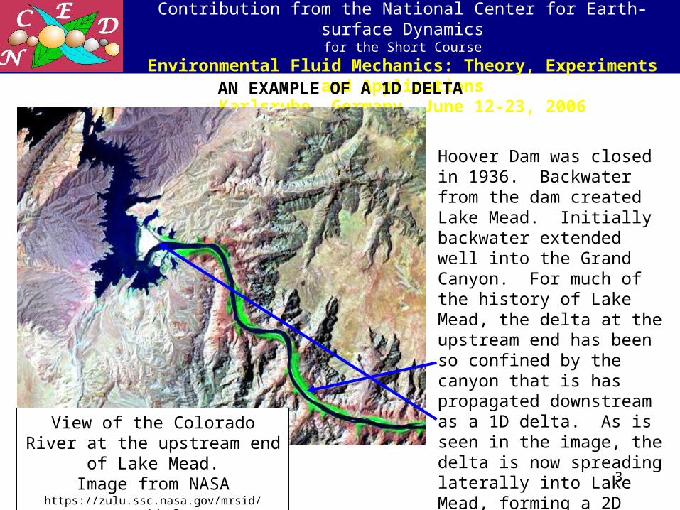
Karlsruhe, Germany, June 12-23, 2006AN EXAMPLE OF A 1D DELTA

Hoover Dam was closed in 1936. Backwater from the dam created Lake Mead. Initially backwater extended well into the Grand Canyon. For much of the history of Lake Mead, the delta at the upstream end has been so confined by the canyon that is has propagated downstream as a 1D delta. As is seen in the image, the delta is now spreading laterally into Lake Mead, forming a 2D fan-delta.

View of the Colorado River at the upstream end of Lake

Mead.Image from NASA

https://zulu.ssc.nasa.gov/mrsid/mrsid.pl

4




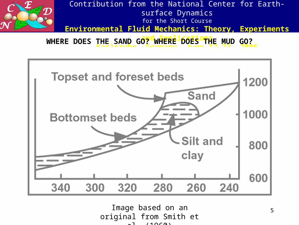
Karlsruhe, Germany, June 12-23, 2006HISTORY OF SEDIMENTATION IN LAKE MEAD, 1936 - 1948

Image based on an original from Smith et al. (1960)

5




Karlsruhe, Germany, June 12-23, 2006WHERE DOES THE SAND GO? WHERE DOES THE MUD GO?

Image based on an original from Smith et al. (1960)

6




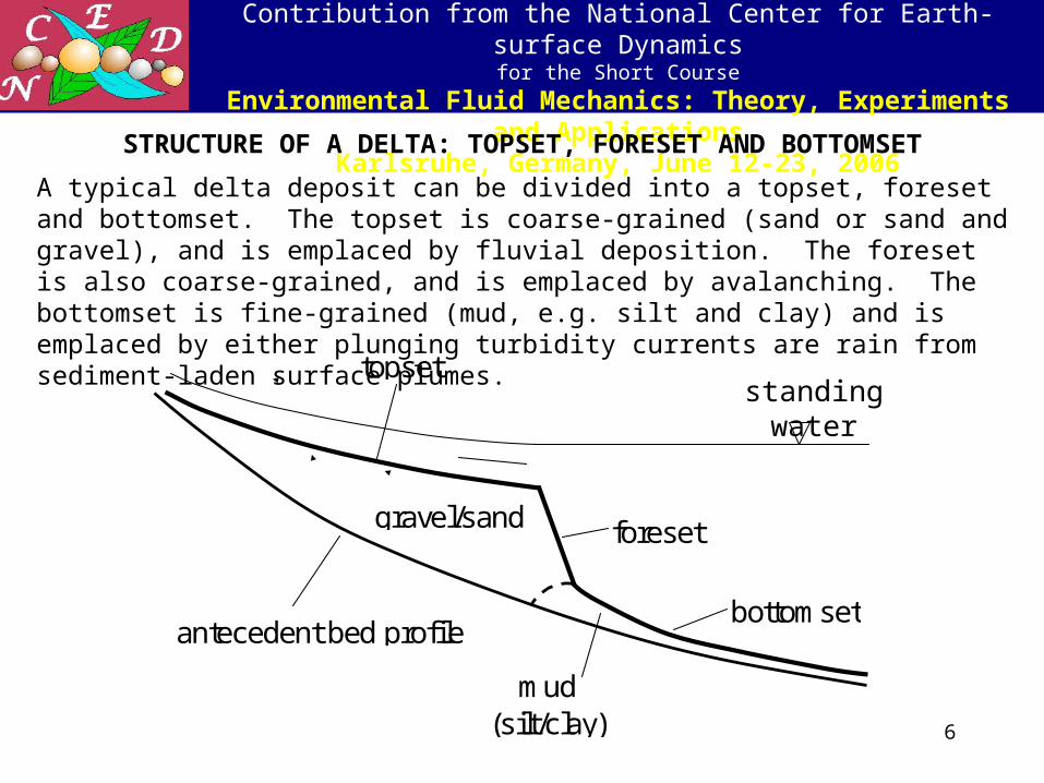
Karlsruhe, Germany, June 12-23, 2006STRUCTURE OF A DELTA: TOPSET, FORESET AND BOTTOMSET

A typical delta deposit can be divided into a topset, foreset and bottomset. The topset is coarse-grained (sand or sand and gravel), and is emplaced by fluvial deposition. The foreset is also coarse-grained, and is emplaced by avalanching. The bottomset is fine-grained (mud, e.g. silt and clay) and is emplaced by either plunging turbidity currents are rain from sediment-laden surface plumes.

antecedent bed profile

topset

foreset

bottomset

gravel/sand

mud(silt/clay)

standing water

7




Karlsruhe, Germany, June 12-23, 2006

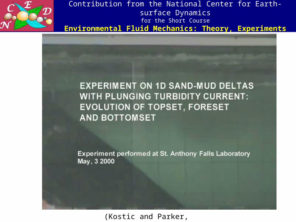
(Kostic and Parker, 2003a,b)

8




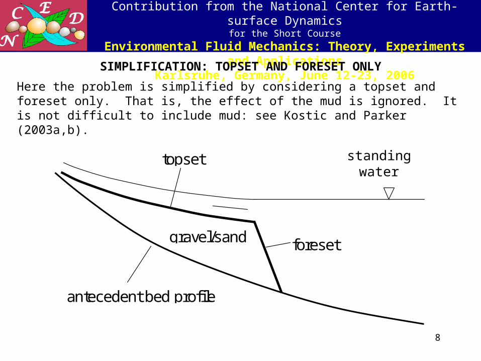
Karlsruhe, Germany, June 12-23, 2006SIMPLIFICATION: TOPSET AND FORESET ONLY

Here the problem is simplified by considering a topset and foreset only. That is, the effect of the mud is ignored. It is not difficult to include mud: see Kostic and Parker (2003a,b).

antecedent bed profile

topset

foresetgravel/sand

standing water

9




Karlsruhe, Germany, June 12-23, 2006DERIVATION OF THE 1D EXNER EQUATION OF SEDIMENT

CONSERVATION

1qq1x)1(t xxtxtsps

The channel has a constant width. Let x = streamwise distance, t = time, qt = the volume sediment transport rate per unit width and p = bed porosity (fraction of bed volume that is pores rather than sediment). The mass sediment transport rate per unit width is then sqt, where s is the material density of sediment. Mass conservation within a control volume with length x and a unit width (Exner, 1920, 1925) requires that:

x

q

t)1( t

p

-

/t (sediment mass in bed of control volume) = mass sediment inflow rate – mass sediment outflow rate

or

or

1x

qt qt

H

x+xx

control volume

10




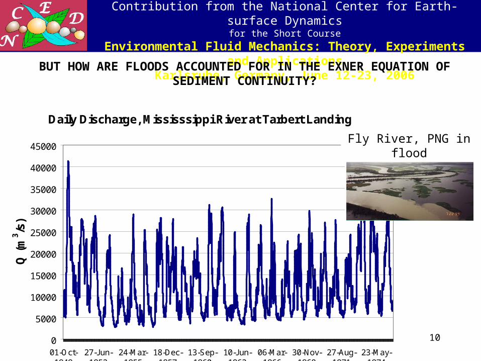
Karlsruhe, Germany, June 12-23, 2006BUT HOW ARE FLOODS ACCOUNTED FOR IN THE EXNER EQUATION OF

SEDIMENT CONTINUITY?

Daily Discharge, Mississsippi River at Tarbert Landing

0

5000

10000

15000

20000

25000

30000

35000

40000

45000

01-Oct-1949

27-Jun-1952

24-Mar-1955

18-Dec-1957

13-Sep-1960

10-Jun-1963

06-Mar-1966

30-Nov-1968

27-Aug-1971

23-May-1974

Q (

m3/s

)

Fly River, PNG in flood

11




Karlsruhe, Germany, June 12-23, 2006SIMPLE ADAPTATION TO ACCOUNT FOR FLOODING

Rivers move the great majority of their sediment, and are morphodynamically active during floods. Paola et al. (1992) represent this in terms of a flood intermittency If. They characterize floods in terms of bankfull flow, which carries a volume bed material transport rate per unit width qt for whatever fraction of time is necessary is necessary to carry the mean annual load of the river. That is, where Gma is the mean annual bed material load of the river, Bbf is bankfull width and Ta is the time of one year, If is adjusted so that

where = water density. The river is assumed to be morphodynamically inactive at other times. Wright and Parker (2005a,b) offer a specific methodology to estimate If.

The Exner equation is thus modified to

x

qI

t)1( t

fp

atbffatbffsma TqBI)R1(TqBIG

12




Karlsruhe, Germany, June 12-23, 2006KEY FEATURES OF THE MORPHODYNAMICS OF THE SELF-EVOLUTION OF 1D

SAND-BED DELTAS UNDER THE INFLUENCE WITH BACKWATER

Water discharge per unit width qw is conserved, and is given by the relation

and shear stress is related to flow velocity using a Chezy (recall Cf-1/2 = C) or

Manning-Strickler formulation;

In low-slope sand-bed streams boundary shear stress cannot be computed from from the depth-slope product, but instead must be obtained from the full backwater equation;

or thus

UHqw

)StricklerManning(k

HCor)Chezy(constC,UC

6/1

cr

2/1ff

2fb

gHSb Hxg

x

Hg

x

UU

t

U b

,

gHq

1

gHq

CS

x

H

3

2w

3

2w

f

2

2wf

2

2w

f2

fb RgDH

qC,

H

qCUC

13




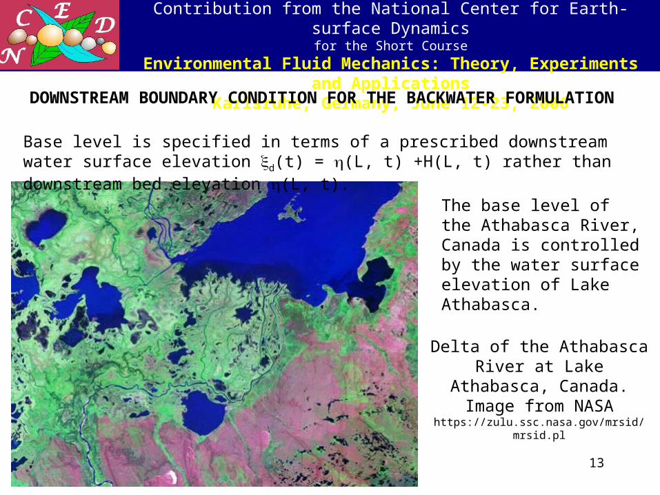
Karlsruhe, Germany, June 12-23, 2006DOWNSTREAM BOUNDARY CONDITION FOR THE BACKWATER FORMULATION

Base level is specified in terms of a prescribed downstream water surface elevation d(t) = (L, t) +H(L, t) rather than downstream bed elevation (L, t).

The base level of the Athabasca River, Canada is controlled by the water surface elevation of Lake Athabasca.

Delta of the Athabasca River at Lake Athabasca,

Canada.Image from NASA

https://zulu.ssc.nasa.gov/mrsid/mrsid.pl

14




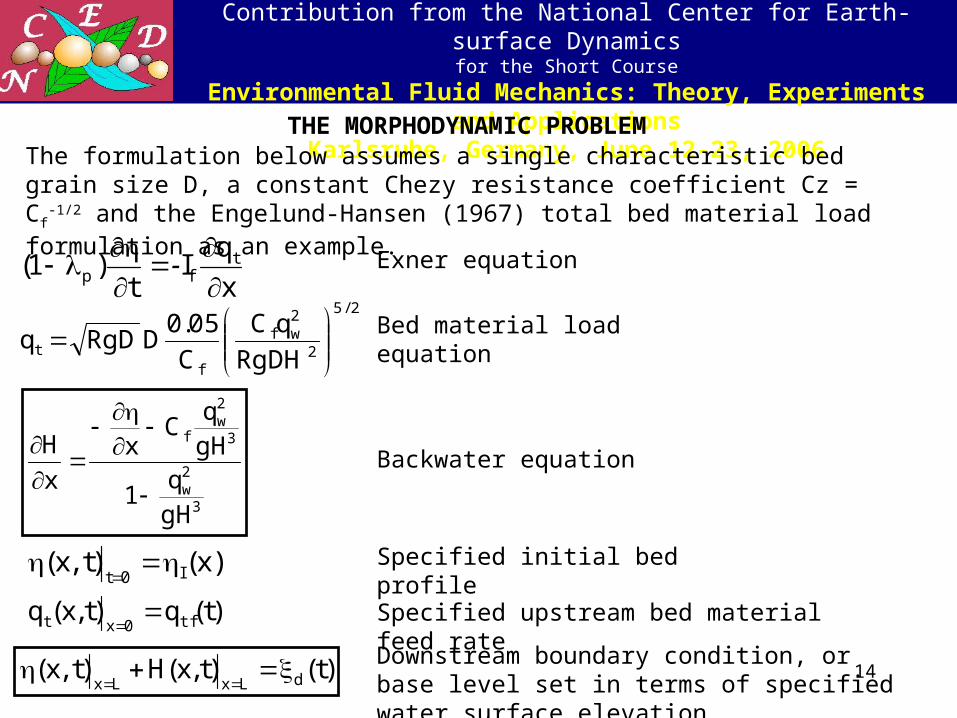
Karlsruhe, Germany, June 12-23, 2006THE MORPHODYNAMIC PROBLEM

x

qI

t)1( t

fp

-2/5

2

2wf

ft RgDH

qC

C

05.0DRgDq

3

2w

3

2w

f

gHq

1

gHq

Cx

x

H

The formulation below assumes a single characteristic bed grain size D, a constant Chezy resistance coefficient Cz = Cf

-1/2 and the Engelund-Hansen (1967) total bed material load formulation as an example.

)x()t,x( I0t

)t(q)t,x(q tf0xt

)t()t,x(H)t,x( dLxLx

Exner equation

Bed material load equation

Backwater equation

Specified initial bed profile

Specified upstream bed material feed rate

Downstream boundary condition, or base level set in terms of specified water surface elevation.

15




Karlsruhe, Germany, June 12-23, 2006NUMERICAL SOLUTION TO THE BACKWATER FORMULATION OF

MORPHODYNAMICS

)t,L()t()t,L(H d

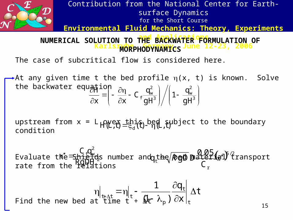
The case of subcritical flow is considered here.

At any given time t the bed profile (x, t) is known. Solve the backwater equation

upstream from x = L over this bed subject to the boundary condition

Evaluate the Shields number and the bed material transport rate from the relations

Find the new bed at time t + t

Repeat using the bed at t + t

2/5

rt C

05.0DgDq R

tx

q

)1(

1

t

t

pttt

3

2w

3

2w

f gHq

1gHq

Cxx

H

2

2wf

RgDH

qC

16





x

qI

t)1( t

fp

)H(1

)H(SS

dx

dH2f

Fr

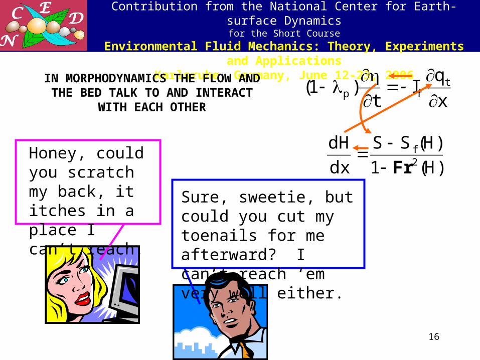
Honey, could you scratch my back, it itches in a place I can’t reach.

Sure, sweetie, but could you cut my toenails for me afterward? I can’t reach ‘em very well either.

IN MORPHODYNAMICS THE FLOW AND THE BED TALK TO AND

INTERACT WITH EACH OTHER

17





antecedent equilibrium bed profile established with load qsa

before raising base level

water surface elevation (base level) is raised at t = 0 by e.g.

installation of a dam

sediment supply remains constant

at qsa

THE PROBLEM OF IMPULSIVELY RAISED WATER SURFACE ELEVATION (BASE LEVEL) AT t = 0

M1 backwater curve

Note: the M1 backwater curve was introduced in the lecture on hydraulics and sediment transport

qta

qta

18




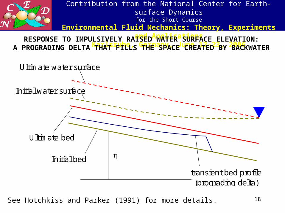
Karlsruhe, Germany, June 12-23, 2006RESPONSE TO IMPULSIVELY RAISED WATER SURFACE ELEVATION:

A PROGRADING DELTA THAT FILLS THE SPACE CREATED BY BACKWATER

Initial bed

transient bed profile (prograding delta)

Ultimate bed

Initial water surface

Ultimate water surface

See Hotchkiss and Parker (1991) for more details.

19




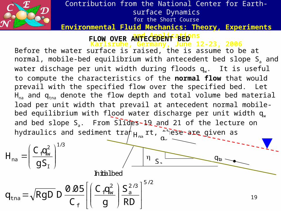
Karlsruhe, Germany, June 12-23, 2006FLOW OVER ANTECEDENT BED

Before the water surface is raised, the is assume to be at normal, mobile-bed equilibrium with antecedent bed slope Sa and water dischage per unit width during floods qw. It is useful to compute the characteristics of the normal flow that would prevail with the specified flow over the specified bed. Let Hna and qtna denote the flow depth and total volume bed material load per unit width that prevail at antecedent normal mobile-bed equilibrium with flood water discharge per unit width qw and bed slope Sa. From Slides 19 and 21 of the lecture on hydraulics and sediment transport, these are given as

3/1

I

2wf

na gS

qCH

2/53/2

a2wf

ftna RD

S

g

qC

C

05.0DRgDq

Initial bed

Hna qw

qtaSa

20




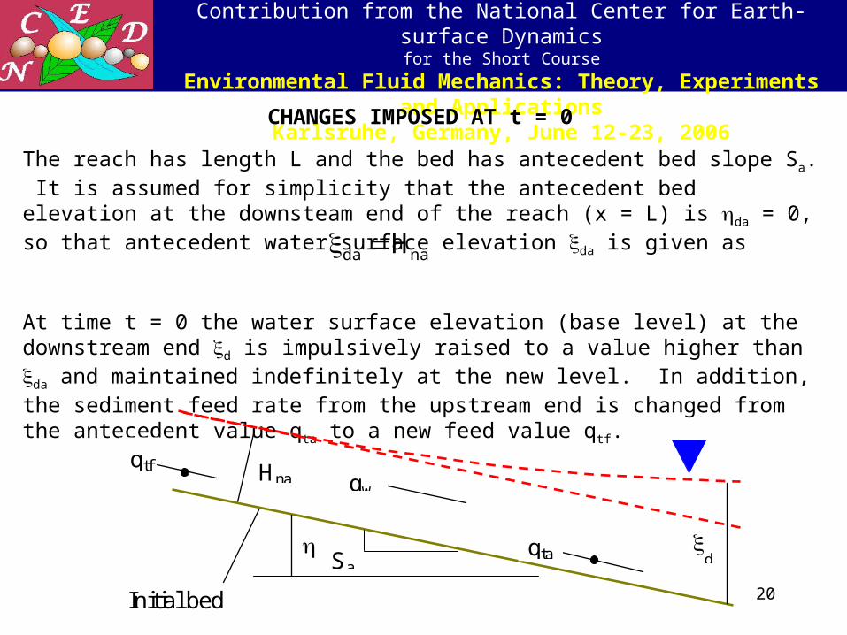
Karlsruhe, Germany, June 12-23, 2006CHANGES IMPOSED AT t = 0

The reach has length L and the bed has antecedent bed slope Sa. It is assumed for simplicity that the antecedent bed elevation at the downsteam end of the reach (x = L) is da = 0, so that antecedent water surface elevation da is given as

At time t = 0 the water surface elevation (base level) at the downstream end d is impulsively raised to a value higher than da and maintained indefinitely at the new level. In addition, the sediment feed rate from the upstream end is changed from the antecedent value qta to a new feed value qtf.

nada H

Initial bed

Hna qw

qtaSa

d

qtf

21




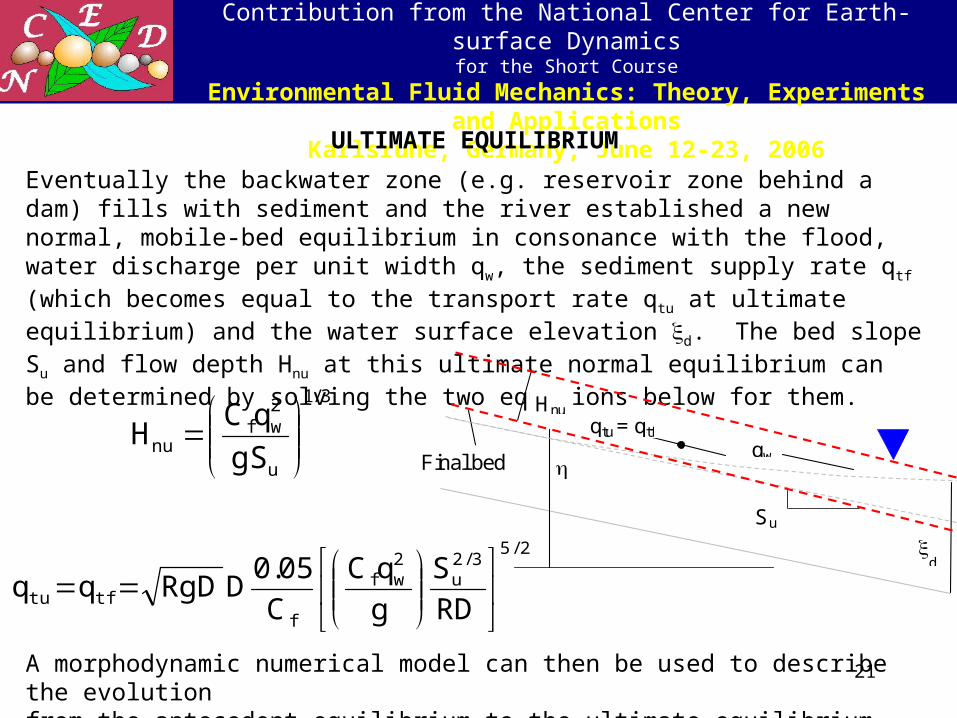
Karlsruhe, Germany, June 12-23, 2006ULTIMATE EQUILIBRIUM

Eventually the backwater zone (e.g. reservoir zone behind a dam) fills with sediment and the river established a new normal, mobile-bed equilibrium in consonance with the flood, water discharge per unit width qw, the sediment supply rate qtf (which becomes equal to the transport rate qtu at ultimate equilibrium) and the water surface elevation d. The bed slope Su and flow depth Hnu at this ultimate normal equilibrium can be determined by solving the two equations below for them.

A morphodynamic numerical model can then be used to describe the evolutionfrom the antecedent equilibrium to the ultimate equilibrium

3/1

u

2wf

nu gS

qCH

2/53/2

u2wf

ftftu RD

S

g

qC

C

05.0DRgDqq

Hnu

qw

qtu = qtf

Su

d

Final bed

22




Karlsruhe, Germany, June 12-23, 2006NUMERICAL MODEL: INITIAL AND BOUNDARY CONDITIONS

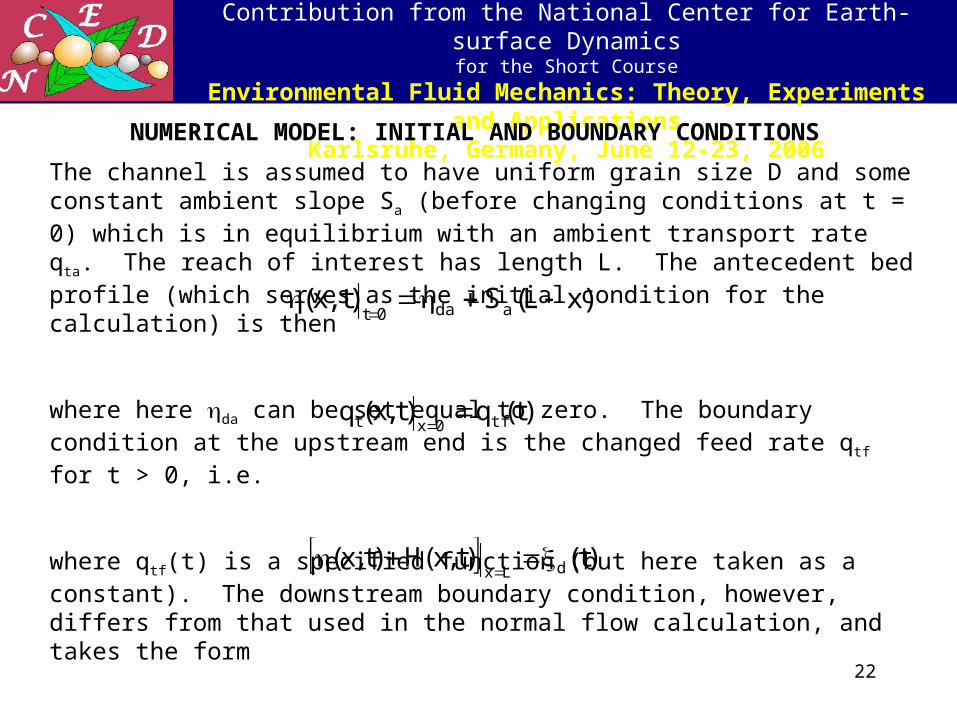
The channel is assumed to have uniform grain size D and some constant ambient slope Sa (before changing conditions at t = 0) which is in equilibrium with an ambient transport rate qta. The reach of interest has length L. The antecedent bed profile (which serves as the initial condition for the calculation) is then

where here da can be set equal to zero. The boundary condition at the upstream end is the changed feed rate qtf for t > 0, i.e.

where qtf(t) is a specified function (but here taken as a constant). The downstream boundary condition, however, differs from that used in the normal flow calculation, and takes the form

where d(t) is in general a specified function, but is here taken to be a constant.

Note that downstream bed elevation (L,t) is not specified, and is free to vary during morphodynamic evolution.

)xL(S)t,x( ada0t

)t(q)t,x(q tf0xt

)t()t,x(H)t,x( dLx

23




Karlsruhe, Germany, June 12-23, 2006NUMERICAL MODEL: DISCRETIZATION AND BACKWATER CURVE

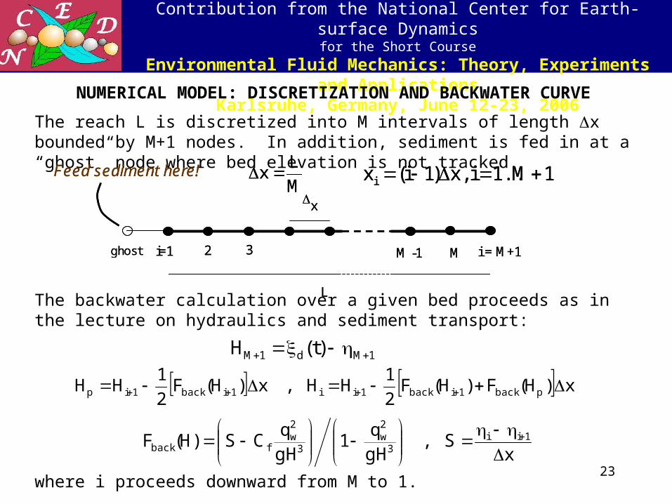
The reach L is discretized into M intervals of length x bounded by M+1 nodes. In addition, sediment is fed in at a “ghost” node where bed elevation is not tracked.

M

Lx 1M..1i,x)1i(x i Feed sediment here!

L

x

i=1 2 3 M -1 i = M+1ghost M

M

Lx 1M..1i,x)1i(x i Feed sediment here!

L

x

i=1 2 3 M -1 i = M+1ghost M

The backwater calculation over a given bed proceeds as in the lecture on hydraulics and sediment transport:

where i proceeds downward from M to 1.

1Md1M )t(H

x)H(F)H(F2

1HH,x)H(F

2

1HH pback1iback1ii1iback1ip

xS,

gHq

1gHq

CS)H(F 1ii3

2w

3

2w

fback

24





1M..1i,tIx

q

1

1f

i,t

ptitti

1Mi,x

qq

M..1i,x

qq)a1(

x

qqa

x

q

1i,ti,t

i,t1i,tu

1i,ti,tu

i,t

)t(qqq tf0,tg,t

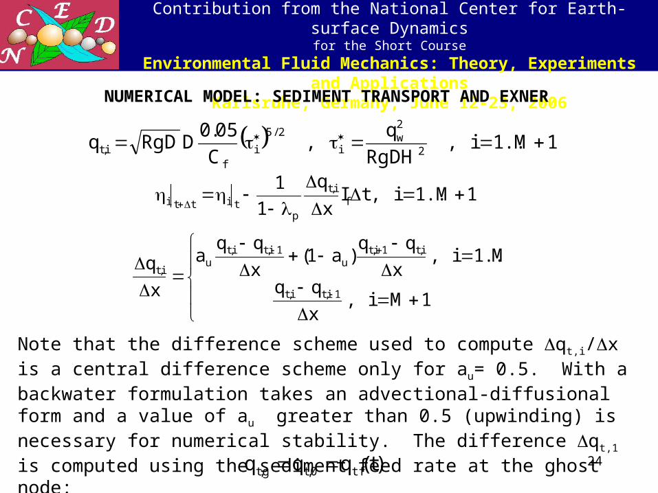
Note that the difference scheme used to compute qt,i/x is a central difference scheme only for au= 0.5. With a backwater formulation takes an advectional-diffusional form and a value of au greater than 0.5 (upwinding) is necessary for numerical stability. The difference qt,1 is computed using the sediment feed rate at the ghost node:

1M..1i,RgDH

q,

C

05.0DRgDq

2

2w

i

2/5

if

i,t

NUMERICAL MODEL: SEDIMENT TRANSPORT AND EXNER

25




Karlsruhe, Germany, June 12-23, 2006INTRODUCTION TO RTe-bookAgDegBWChezy.xls

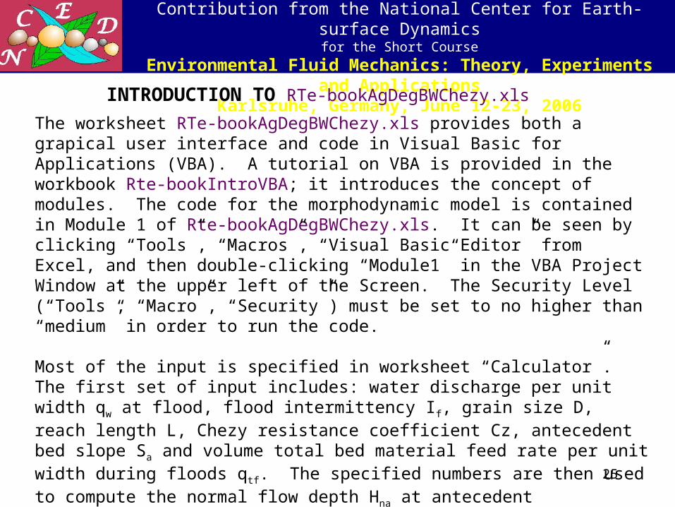
The worksheet RTe-bookAgDegBWChezy.xls provides both a grapical user interface and code in Visual Basic for Applications (VBA). A tutorial on VBA is provided in the workbook Rte-bookIntroVBA; it introduces the concept of modules. The code for the morphodynamic model is contained in Module 1 of Rte-bookAgDegBWChezy.xls. It can be seen by clicking “Tools”, “Macros”, “Visual Basic Editor” from Excel, and then double-clicking “Module1” in the VBA Project Window at the upper left of the Screen. The Security Level (“Tools”, “Macro”, “Security”) must be set to no higher than “medium” in order to run the code.

Most of the input is specified in worksheet “Calculator”. The first set of input includes: water discharge per unit width qw at flood, flood intermittency If, grain size D, reach length L, Chezy resistance coefficient Cz, antecedent bed slope Sa and volume total bed material feed rate per unit width during floods qtf. The specified numbers are then used to compute the normal flow depth Hna at antecedent conditions, the final ultimate equilibrium bed slope Su and the final ultimate equilibrium normal flow depth Hnu.

The user then specifies a downstream water surface elevation d. Thisvalue should be > the larger of either Hna or Hnu to cause delta formation.

26




Karlsruhe, Germany, June 12-23, 2006INTRODUCTION TO RTe-bookAgDegBWChezy.xls contd.

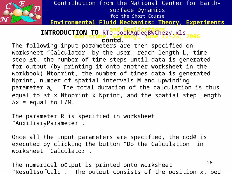
The following input parameters are then specified on worksheet “Calculator” by the user: reach length L, time step t, the number of time steps until data is generated for output (by printing it onto another worksheet in the workbook) Ntoprint, the number of times data is generated Nprint, number of spatial intervals M and upwinding parameter au. The total duration of the calculation is thus equal to t x Ntoprint x Nprint, and the spatial step length x = equal to L/M.

The parameter R is specified in worksheet “AuxiliaryParameter”.

Once all the input parameters are specified, the code is executed by clicking the button “Do the Calculation” in worksheet “Calculator”.

The numerical output is printed onto worksheet “ResultsofCalc”. The output consists of the position x, bed elevation , water surface elevation and flow depth H at every node for time t = 0 and Nprint subsequent times. The bed elevations and final water surface elevations are plotted on worksheet “PlottheData”.

27




Karlsruhe, Germany, June 12-23, 2006INTRODUCTION TO RTe-bookAgDegBWChezy.xls contd.

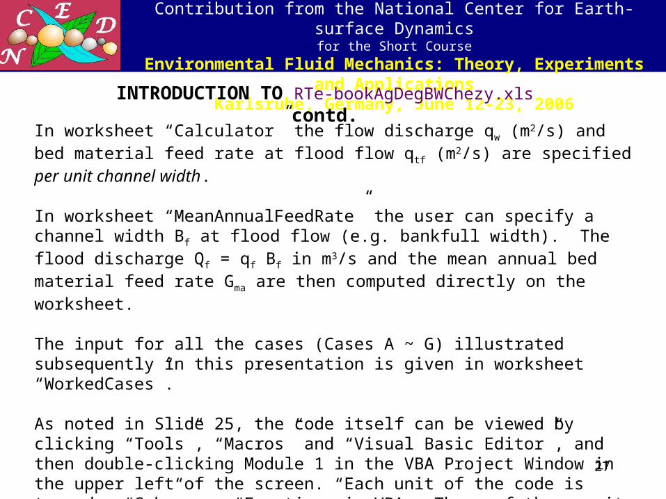
In worksheet “Calculator” the flow discharge qw (m2/s) and bed material feed rate at flood flow qtf (m2/s) are specified per unit channel width.

In worksheet “MeanAnnualFeedRate” the user can specify a channel width Bf at flood flow (e.g. bankfull width). The flood discharge Qf = qf Bf in m3/s and the mean annual bed material feed rate Gma are then computed directly on the worksheet.

The input for all the cases (Cases A ~ G) illustrated subsequently in this presentation is given in worksheet “WorkedCases”.

As noted in Slide 25, the code itself can be viewed by clicking “Tools”, “Macros” and “Visual Basic Editor”, and then double-clicking Module 1 in the VBA Project Window in the upper left of the screen. Each unit of the code is termed a “Sub” or a “Function” in VBA. Three of these units are illustrated in Slides 29, 30 and 31.

28




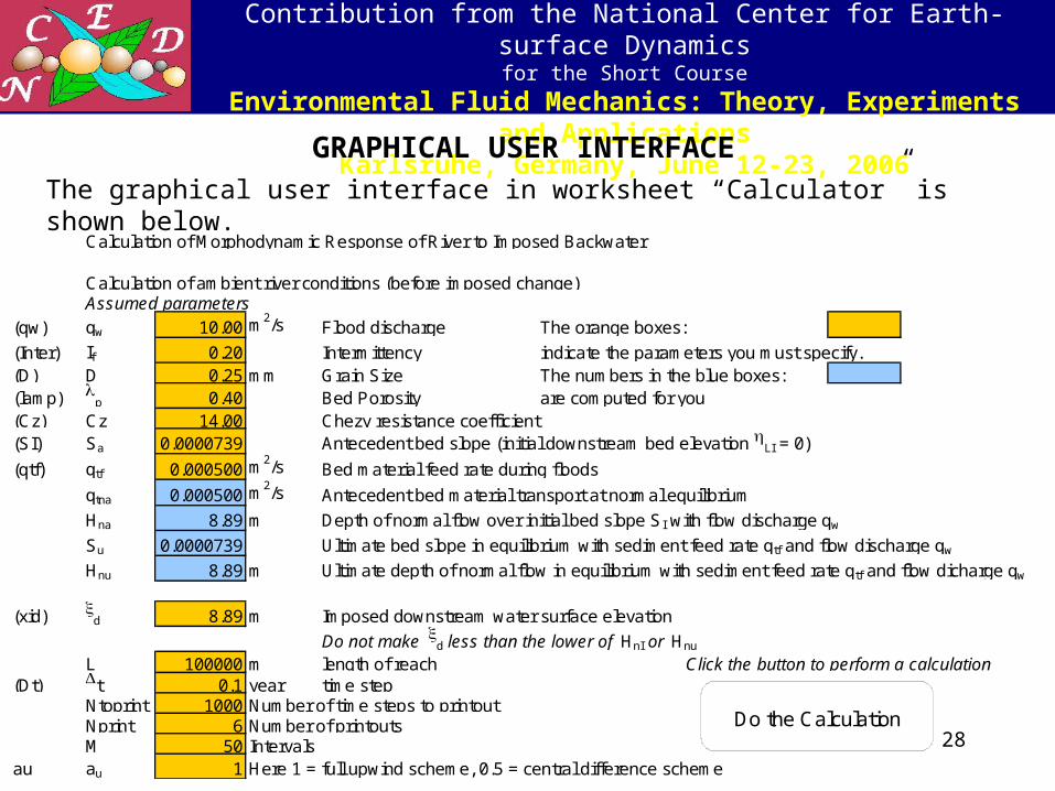
Karlsruhe, Germany, June 12-23, 2006GRAPHICAL USER INTERFACE

The graphical user interface in worksheet “Calculator” is shown below.

Calculation of Morphodynamic Response of River to Imposed Backwater

Calculation of ambient river conditions (before imposed change)Assumed parameters

(qw) qw 10.00 m2/s Flood discharge The orange boxes:

(Inter) If 0.20 Intermittency indicate the parameters you must specify.(D) D 0.25 mm Grain Size The numbers in the blue boxes:(lamp)

p 0.40 Bed Porosity are computed for you(Cz) Cz 14.00 Chezy resistance coefficient(SI) Sa 0.0000739 Antecedent bed slope (initial downstream bed elevation LI = 0)

(qtf) qtf 0.000500 m2/s Bed material feed rate during floods

qtna 0.000500 m2/s Antecedent bed material transport at normal equilibrium

Hna 8.89 m Depth of normal flow over initial bed slope SI with flow discharge qw

Su 0.0000739 Ultimate bed slope in equilibrium with sediment feed rate qtf and flow discharge qw

Hnu 8.89 m Ultimate depth of normal flow in equilibrium with sediment feed rate q tf and flow dicharge qw

(xid) d 8.89 m Imposed downstream water surface elevation

Do not make d less than the lower of HnI or Hnu

L 100000 m length of reach Click the button to perform a calculation(Dt) t 0.1 year time step

Ntoprint 1000 Number of time steps to printoutNprint 6 Number of printoutsM 50 Intervals

au au 1 Here 1 = full upwind scheme, 0.5 = central difference scheme

Do the Calculation

29




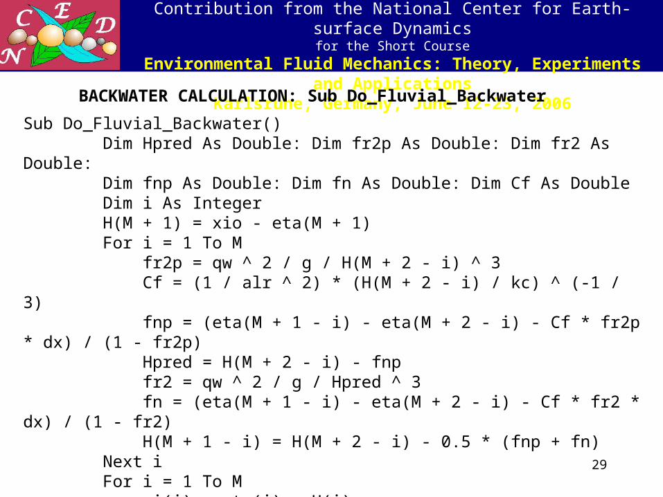
Karlsruhe, Germany, June 12-23, 2006Sub Do_Fluvial_Backwater() Dim Hpred As Double: Dim fr2p As Double: Dim fr2 As Double: Dim fnp As Double: Dim fn As Double: Dim Cf As Double Dim i As Integer H(M + 1) = xio - eta(M + 1) For i = 1 To M fr2p = qw ^ 2 / g / H(M + 2 - i) ^ 3 Cf = (1 / alr ^ 2) * (H(M + 2 - i) / kc) ^ (-1 / 3) fnp = (eta(M + 1 - i) - eta(M + 2 - i) - Cf * fr2p * dx) / (1 - fr2p) Hpred = H(M + 2 - i) - fnp fr2 = qw ^ 2 / g / Hpred ^ 3 fn = (eta(M + 1 - i) - eta(M + 2 - i) - Cf * fr2 * dx) / (1 - fr2) H(M + 1 - i) = H(M + 2 - i) - 0.5 * (fnp + fn) Next i For i = 1 To M xi(i) = eta(i) + H(i) Next i End Sub

BACKWATER CALCULATION: Sub Do_Fluvial_Backwater

30





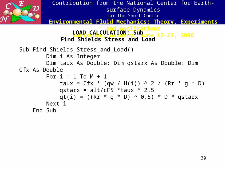
Sub Find_Shields_Stress_and_Load() Dim i As Integer Dim taux As Double: Dim qstarx As Double: Dim Cfx As Double For i = 1 To M + 1 taux = Cfx * (qw / H(i)) ^ 2 / (Rr * g * D) qstarx = alt/cFS *taux ^ 2.5 qt(i) = ((Rr * g * D) ^ 0.5) * D * qstarx Next i End Sub

LOAD CALCULATION: Sub Find_Shields_Stress_and_Load

31





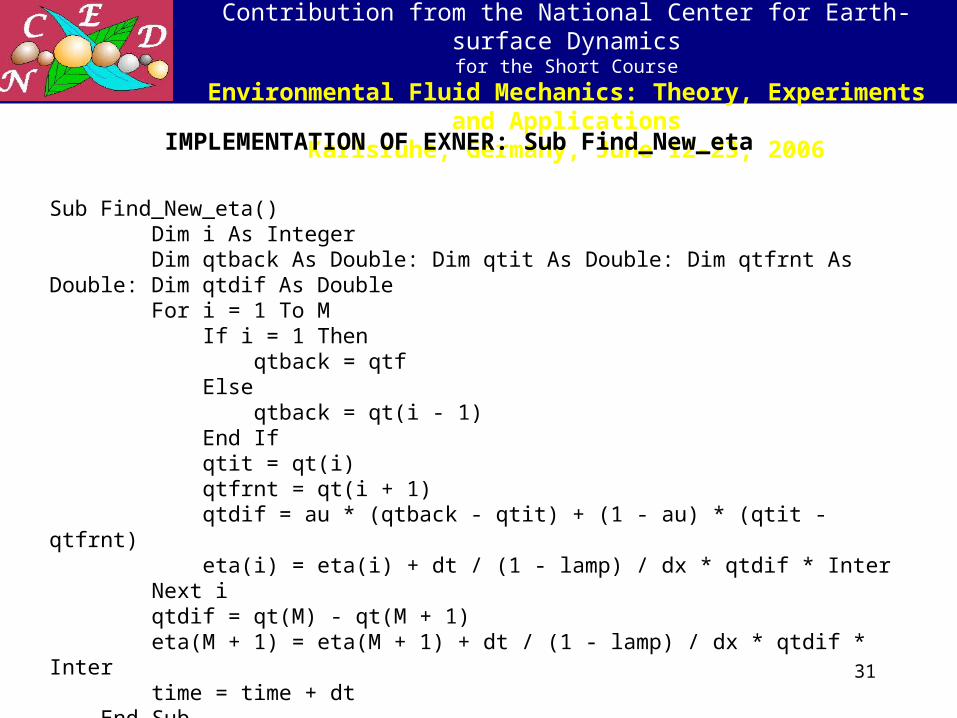
Sub Find_New_eta() Dim i As Integer Dim qtback As Double: Dim qtit As Double: Dim qtfrnt As Double: Dim qtdif As Double For i = 1 To M If i = 1 Then qtback = qtf Else qtback = qt(i - 1) End If qtit = qt(i) qtfrnt = qt(i + 1) qtdif = au * (qtback - qtit) + (1 - au) * (qtit - qtfrnt) eta(i) = eta(i) + dt / (1 - lamp) / dx * qtdif * Inter Next i qtdif = qt(M) - qt(M + 1) eta(M + 1) = eta(M + 1) + dt / (1 - lamp) / dx * qtdif * Inter time = time + dt End Sub

IMPLEMENTATION OF EXNER: Sub Find_New_eta

32




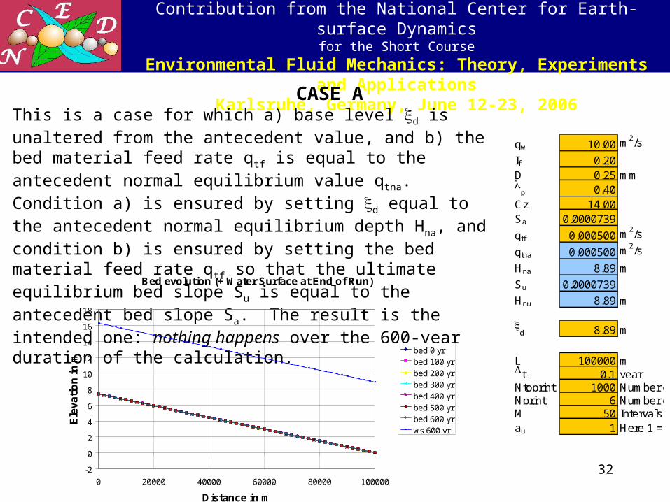
Karlsruhe, Germany, June 12-23, 2006CASE A

This is a case for which a) base level d is unaltered from the antecedent value, and b) the bed material feed rate qtf is equal to the antecedent normal equilibrium value qtna. Condition a) is ensured by setting d equal to the antecedent normal equilibrium depth Hna, and condition b) is ensured by setting the bed material feed rate qtf so that the ultimate equilibrium bed slope Su is equal to the antecedent bed slope Sa. The result is the intended one: nothing happens over the 600-year duration of the calculation. Bed evolution (+ Water Surface at End of Run)

-2

0

2

4

6

8

10

12

14

16

18

0 20000 40000 60000 80000 100000

Distance in m

Ele

vati

on

in m

bed 0 yrbed 100 yrbed 200 yrbed 300 yrbed 400 yrbed 500 yrbed 600 yrws 600 yr

qw 10.00 m2/s

If 0.20D 0.25 mm

p 0.40Cz 14.00Sa 0.0000739

qtf 0.000500 m2/s

qtna 0.000500 m2/s

Hna 8.89 m

Su 0.0000739

Hnu 8.89 m

d 8.89 m

L 100000 mt 0.1 yearNtoprint 1000 Number of time steps to printoutNprint 6 Number of printoutsM 50 Intervalsau 1 Here 1 = full upwind scheme, 0.5 = central difference scheme

33




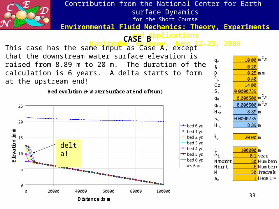
Karlsruhe, Germany, June 12-23, 2006CASE B

This case has the same input as Case A, except that the downstream water surface elevation is raised from 8.89 m to 20 m. The duration of the calculation is 6 years. A delta starts to form at the upstream end!

Bed evolution (+ Water Surface at End of Run)

0

5

10

15

20

25

0 20000 40000 60000 80000 100000

Distance in m

Ele

vati

on

in m


qw 10.00 m2/s

If 0.20D 0.25 mm

p 0.40Cz 14.00Sa 0.0000739

qtf 0.000500 m2/s

qtna 0.000500 m2/s

Hna 8.89 m

Su 0.0000739

Hnu 8.89 m

d 20.00 m


delta!

34




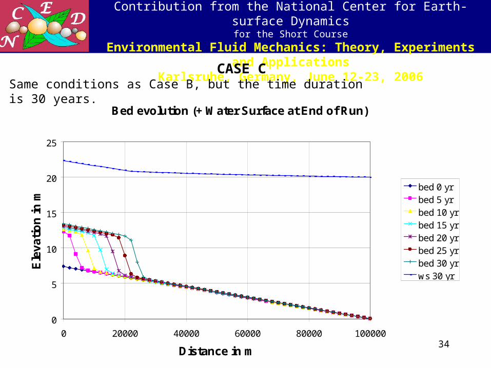
Karlsruhe, Germany, June 12-23, 2006CASE C

Same conditions as Case B, but the time duration is 30 years.


0

5

10

15

20

25

0 20000 40000 60000 80000 100000

Distance in m

Ele

vati

on

in m


35




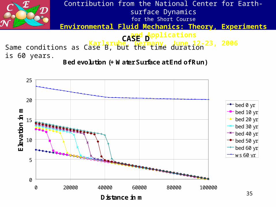
Karlsruhe, Germany, June 12-23, 2006CASE D



0

5

10

15

20

25

0 20000 40000 60000 80000 100000

Distance in m

Ele

vati

on

in m


36




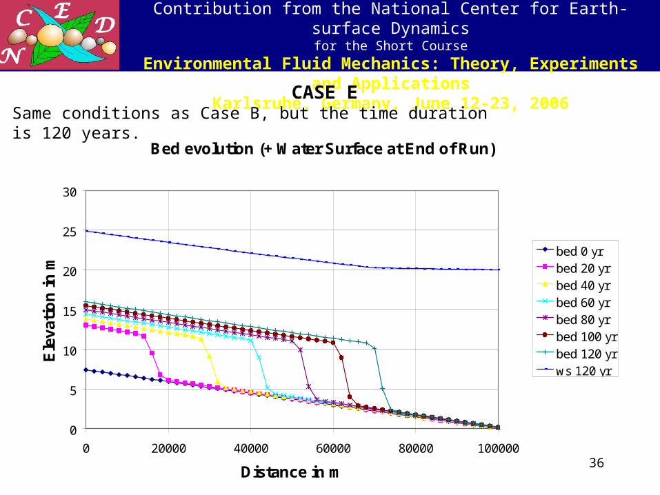
Karlsruhe, Germany, June 12-23, 2006CASE E



0

5

10

15

20

25

30

0 20000 40000 60000 80000 100000

Distance in m

Ele

vati

on

in m


37




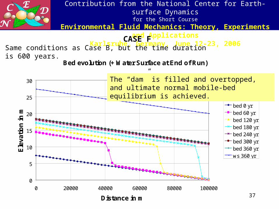
Karlsruhe, Germany, June 12-23, 2006CASE F



0

5

10

15

20

25

30

0 20000 40000 60000 80000 100000

Distance in m

Ele

vati

on

in m


The “dam” is filled and overtopped, and ultimate normal mobile-bed equilibrium is achieved.

38




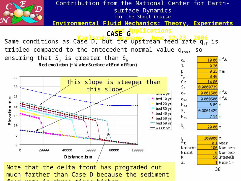
Karlsruhe, Germany, June 12-23, 2006CASE G

Same conditions as Case D, but the upstream feed rate qtf is tripled compared to the antecedent normal value qtna, so ensuring that Su is greater than Sa


0

5

10

15

20

25

30

35

0 20000 40000 60000 80000 100000

Distance in m

Ele

vati

on

in m


qw 10.00 m2/s

If 0.20D 0.25 mm

p 0.40Cz 14.00Sa 0.0000739

qtf 0.001500 m2/s

qtna 0.000500 m2/s

Hna 8.89 m

Su 0.0001429

Hnu 7.14 m

d 20.00 m


This slope is steeper than this slope

Note that the delta front has prograded out much farther than Case D because the sediment feed rate is three times higher.

39




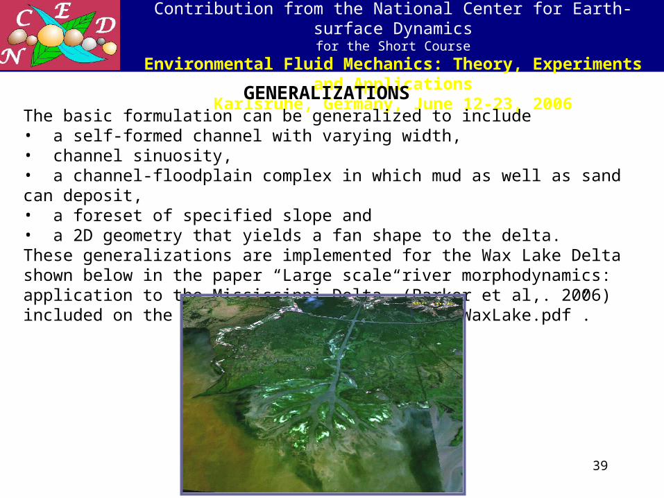
Karlsruhe, Germany, June 12-23, 2006GENERALIZATIONS

The basic formulation can be generalized to include• a self-formed channel with varying width,• channel sinuosity,• a channel-floodplain complex in which mud as well as sand can deposit,• a foreset of specified slope and• a 2D geometry that yields a fan shape to the delta.These generalizations are implemented for the Wax Lake Delta shown below in the paper “Large scale river morphodynamics: application to the Mississippi Delta” (Parker et al,. 2006) included on the CD for this course as file “WaxLake.pdf”.

40




Karlsruhe, Germany, June 12-23, 2006REFERENCES

Exner, F. M., 1920, Zur Physik der Dunen, Sitzber. Akad. Wiss Wien, Part IIa, Bd. 129 (in German).

Exner, F. M., 1925, Uber die Wechselwirkung zwischen Wasser und Geschiebe in Flussen, Sitzber. Akad. Wiss Wien, Part IIa, Bd. 134 (in German).

Hotchkiss, R. H. and Parker, G., 1991, Shock fitting of aggradational profiles due to backwater, Journal of Hydraulic Engineering, 117(9): 1129‑1144.

Kostic, S. and Parker, G., 2003a, Progradational sand-mud deltas in lakes and reservoirs. Part 1. Theory and numerical modeling, Journal of Hydraulic Research, 41(2), pp. 127-140.

Kostic, S. and Parker, G.. 2003b, Progradational sand-mud deltas in lakes and reservoirs. Part 2. Experiment and numerical simulation, Journal of Hydraulic Research, 41(2), pp. 141-152.

Paola, C., Heller, P. L. & Angevine, C. L., 1992, The large-scale dynamics of grain-size variation in alluvial basins. I: Theory, Basin Research, 4, 73-90.

Parker, G., Sequeiros, O. and River Morphodynamics Class of Spring 2006, 2006, Large scale river morphodynamics: application to the Mississippi Delta, Proceedings, River Flow 2006 Conference, Lisbon, Portugal, September 6 – 8, 2006, Balkema.

Smith, W. O., Vetter, C.P. and Cummings, G. B., 1960, Comprehensive survey of Lake Mead, 1948-1949: Professional Paper 295, U.S. Geological Survey, 254 p.

Wright, S. and Parker, G., 2005a, Modeling downstream fining in sand-bed rivers. I: Formulation, Journal of Hydraulic Research, 43(6), 612-619.

Wright, S. and Parker, G., 2005b, Modeling downstream fining in sand-bed rivers. II: Application, Journal of Hydraulic Research, 43(6), 620-630.

Documents

MORPHODYNAMICS OF SAND-BED RIVERS ENDING IN DELTAS