Morphing of Triangular Meshes in Shape Spacecs.smith.edu/~jorourke/Papers/shapeSpace.pdf · 2009-11-19 · Morphing of Triangular Meshes in Shape Space 3 shape space corresponds to

November 18, 2009 21:7 WSPC/INSTRUCTION FILE shapeSpace

International Journal of Shape Modelingc© World Scientific Publishing Company

Morphing of Triangular Meshes in Shape Space∗

Stefanie Wuhrer

National Research Council of Canada, Ottawa, Ontario, [email protected]

Prosenjit Bose

School of Computer Science, Carleton University, Ottawa, Ontario, [email protected]

Chang Shu

National Research Council of Canada, Ottawa, Ontario, [email protected]

Joseph O’Rourke

Smith College, Northampton, USA

[email protected]

Alan Brunton

University of Ottawa, Ottawa, Canada

National Research Council of Canada, Ottawa, [email protected]

Received (Day Month Year)Revised (Day Month Year)

Accepted (Day Month Year)

Communicated by (xxxxxxxxxx)

We present a novel approach to morph between two isometric poses of the same non-rigid object given as triangular meshes. We model the morphs as linear interpolations

in a suitable shape space S. For triangulated 3D polygons, we prove that interpolating

linearly in this shape space corresponds to the most isometric morph in R3. We thenextend this shape space to arbitrary triangulations in 3D using a heuristic approach

and show the practical use of the approach using experiments. Furthermore, we dis-cuss a modified shape space that is useful for isometric skeleton morphing. All of thenewly presented approaches solve the morphing problem without the need to solve a

minimization problem.

Keywords: Morphing, shape space, geometry processing, computational geometry.

∗A preliminary version of this work was accepted to CCCG 2008. Research supported in part by

HPCVL and NSERC.

1


2 S. Wuhrer, P. Bose, C. Shu, J. O’Rourke, and A. Brunton

1. Introduction

Interpolating smoothly between two given poses of the same non-rigid object, knownas morphing, arises from many geometry processing problems. For example, morph-ing can compute an animation between given poses of a human or an animal. Twoobjects are isometric if they have the same intrinsic geometry. We consider morphsbetween isometric objects because the locomotion of humans and many animalspreserves the intrinsic geometry of the body. We aim to solve the following prob-lem. Given two isometric poses of the same non-rigid object as triangular meshesS(0) and S(1) with known point-to-point correspondences, find a smooth isometricdeformation between the poses.

Recently, Kilian et al. 8 showed that an isometric morph can be computed byfinding a geodesic path in a shape space. A mesh that contains n vertices is usuallyrepresented in shape space as a point in R3n that contains all the vertex coordi-nates of the mesh. 7 The mesh is arranged in a standard position so it is translationand rotation invariant. Computing geodesic paths in this space involves solving alarge-scale non-linear optimization problem. Non-linear optimization problems areusually solved iteratively starting from an initial solution. This is computationallyexpensive. It is difficult to find the best solution because convergence problems mayarise if the initial solution is far from the optimum, and finding a good initial solu-tion is not straight forward. Kilian et al. overcome the inefficiency of the approachand the difficulty of finding a good initial solution by implementing two multi-resolution schemes. The number of resolutions that are used have an effect on theresult. This means that the numbers of resolutions can be viewed as non-intuitiveinput parameters. The approach is difficult to implement.

The objective of this paper is to propose an alternative representation of theshape space. Instead of encoding the extrinsic geometry of the mesh in shape spaceas in Kilian et al., we encode the intrinsic geometry of the mesh in shape space.This has the effect that a point on a geodesic path in shape space simply linearlyinterpolates between the endpoints of the geodesic path. Hence, we replace solvinga large-scale non-linear optimization problem with linearly interpolating betweentwo points. This is more efficient, conceptually simpler, and easier to implement.

A deformation of a shape represented by a triangular mesh is isometric if andonly if all triangle edge lengths are preserved during the deformation. 8 We call amorph S(t), 0 < t < 1 between two (possibly non-isometric) shapes S(0) and S(1)

most isometric if it minimizes the sum of the absolute values of the differencesbetween the corresponding edge lengths of two consecutive shapes summed over allshapes S(t), for t in [0, 1]. Note that in a similar definition, Kilian et al. 8 use the L2

instead of the L1 metric as we do to measure most isometric morphs. In this paper,we examine isometric morphs of general triangular manifold meshes in 3D. We startby examining the simpler problem of morphing between isometric triangulated 3D

polygons, which are triangular meshes with no interior vertices. In this case, weintroduce a new shape space S that has the property that interpolating linearly in


Morphing of Triangular Meshes in Shape Space 3

shape space corresponds to the most isometric morph in R3. For arbitrary triangularmeshes, this property is no longer guaranteed. However, we extend the shape spaceto arbitrary triangular manifold meshes using a heuristic approach. While we cancompute morphs in this shape space using linear interpolations, the morphs are nolonger guaranteed to be of high quality. Furthermore, we discuss a modification ofthe shape space that is useful for isometric skeleton morphing.

2. Related Work

Computing a smooth morph from one pose of a shape in two or three dimensions toanother pose of the same shape has received considerable attention. 10, 2 A recentsurvey on this topic is by Alexa. 1

Early work on morphing has focused on the two-dimensional version of the prob-lem. We focus on the case where the input is sampled over an irregular domain. Inthis case, the problem is to interpolate between two simple polygons in the plane.Several authors make use of intrinsic representations of the polygons. Sederberg etal. 14 proposed to interpolate an intrinsic representation of two-dimensional poly-gons, namely the edge lengths and interior angles of the polygon. Surazhsky andGotsman 20 morphed by computing mean value barycentric coordinates based onan intrinsic representation of triangulated polygons. This method is guaranteed tobe intersection free. Iben et al. 6 morphed planar polygons while guaranteeing thatno self-intersections occur using an approach based on energy minimization. Thisapproach can be constrained to be as isometric as possible. Our approach can beviewed as a generalization of these techniques to three dimensions.

More recently, much work has focused on morphing between triangular meshes.We first review work that does not require energy minimizations. Sun et al. 19 mor-phed between three-dimensional manifold meshes. They extended the approach bySederberg et al. 14 to three dimensions by extending the intrinsic representationto polyhedra. However, the developed methods are computationally expensive. 1

Another extension of the approach by Sederberg et al. 14 to three dimensions waspresented by Lipman et al. 11 They gave a rotation-invariant mesh representationthat is similar in spirit to the first and second fundamental form in differential ge-ometry. This representation can be used to find an approximate morph. The methodis again computationally expensive. Our approach is similar to these approaches inthat no energy is minimized. However, it is more efficient.

Next we review approaches that require solving non-linear optimization prob-lems. When solving non-linear optimization problems, it is often not guaranteedthat a globally optimal solution is found. Kraevoy and Sheffer 9 presented a rep-resentation that is based on mean-value encodings of vertices. This representationhas the property that similar models have similar encodings and it can be used formorphing. Morphing requires minimizing a non-linear energy function. Sorkine andAlexa 17 proposed an algorithm to deform a surface based on a given triangularsurface and updated positions of few feature points. The surface is modeled as a



covering by overlapping cells. The deformation aims to deform each cell as rigidlyas possible. The overlap is necessary to avoid stretching along cell boundaries. Thedeformation is based on minimizing a global non-linear energy function. While theenergy is guaranteed to converge, the algorithm is not guaranteed to find the globalminimum. If the global minimum is found, the approach tends to preserve theedge lengths of the triangular mesh. Zhou et al. 22 proposed a method to deformtriangular meshes based on the Laplacian of a graph representing the volume ofthe triangular mesh. The method is shown to prevent volumetric details to changeunnaturally. The work by Kilian et al. 8 was described in Section 1. In this ap-proach, the geodesic paths in shape space are found using an energy-minimizationapproach. Note that Kilian et al.’s approach is more general than our approach inthat it is possible to extrapolate isometric deformations. Eckstein et al. 4 proposeda generalized gradient descent method similar to the approach by Kilian et al. thatcan be applied to deform triangular meshes.

In this paper, we propose a novel shape space representation for morphing thatdoes not require solving a minimization problem. The representation has the prop-erty that interpolating linearly in shape space approximates the most isometricmorph in R3. For triangulated 3D polygons, we prove that the linear interpola-tion in shape space corresponds exactly to the most isometric morph in R3. Forarbitrary triangulated manifolds in 3D, we provide a heuristic that extends theapproach developed for 3D polygons.

3. Theory of Shape Space for Triangulated 3D Polygons

Before considering the problem of morphing between triangulated manifolds in 3D,we consider the simpler problem of morphing between triangular meshes with nointerior vertices. We call these meshes triangulated 3D polygons in the following.

We start with two triangulated 3D polygons P (0) and P (1) corresponding totwo near-isometric poses of the same non-rigid object. Poses are considered near-isometric if the stretching between the poses is small. We assume that the point-to-point correspondence of the vertices P (0) and P (1) are known. Furthermore, weassume that both P (0) and P (1) share the same underlying mesh structure M .Hence, we know the mesh structure M with two sets of ordered vertex coordinatesV (0) and V (1) in R3, where M is an outer-planar graph. We will show that wecan represent P (0) and P (1) as points p(0) and p(1) in a shape space S, such thateach point p(t) that is a linear interpolation between p(0) and p(1) corresponds to atriangular mesh P (t) isometric to P (0) and P (1) in R3.

As we know the point-to-point correspondence of the vertices P (0) and P (1), wecan find the best rigid alignment of the two shapes by solving an overdeterminedlinear system of equations and by modifying the solution to ensure a valid rotationmatrix. To modify the solution to the overdetermined linear system, we compute asingular value decomposition of the solution matrix and replace the singular valuematrix by the identity matrix. 5 Note that the relative rigid alignment of P (0) and



P (1) in R3 has an influence on the linear interpolation.Let M consist of n vertices. As M is a triangulation of a 3D polygon with n

vertices, M has 2n− 3 edges and n− 2 triangles. We assign an arbitrary but fixedorder on the vertices, edges, and faces of M . The shape space S is defined as follows.The first 3 coordinates of a point p ∈ S correspond to the coordinates of the firstvertex v in M . Coordinates 4 and 5 of p correspond to the direction of the first edgeof M incident to v in spherical coordinates. The next 2n − 3 coordinates of p arethe lengths of the edges in M in order. The final 2(n− 2) coordinates of p describethe outer normal directions of the triangles in M in spherical coordinates, in order.Hence, the shape space S has dimension 5 + 2n− 3 + 2(n− 2) = 4n− 2 = Θ(n).

In the following, we prove that interpolating linearly between P (0) and P (1)

in shape space yields the most isometric morph. To interpolate linearly in shapespace, we interpolate the edge lengths by simple linear interpolation. That is, p

(t)k =

tp(0)k + (1− t)p(1)

k , where p(x)k is the kth coordinate of p(x). The normal vectors are

interpolated using geometric spherical linear interpolation (SLERP). 15 That is,p

(t)k = sin(1−t)Θ

sin Θ p(0)k + sin tΘ

sin Θ p(1)k , where Θ is the angle between the two directions

that are interpolated.To study interpolation in shape space, we make use of the dual graph D(M)

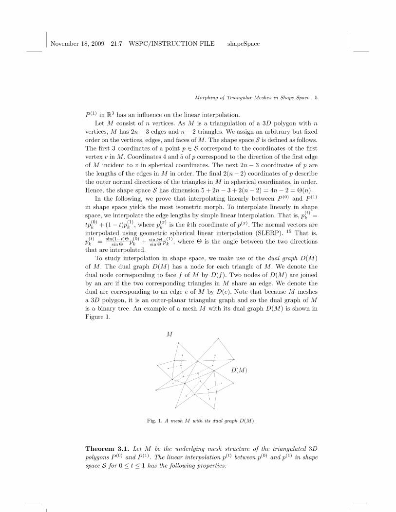
of M . The dual graph D(M) has a node for each triangle of M . We denote thedual node corresponding to face f of M by D(f). Two nodes of D(M) are joinedby an arc if the two corresponding triangles in M share an edge. We denote thedual arc corresponding to an edge e of M by D(e). Note that because M meshesa 3D polygon, it is an outer-planar triangular graph and so the dual graph of M

is a binary tree. An example of a mesh M with its dual graph D(M) is shown inFigure 1.

M

D(M)

Fig. 1. A mesh M with its dual graph D(M).

Theorem 3.1. Let M be the underlying mesh structure of the triangulated 3D

polygons P (0) and P (1). The linear interpolation p(t) between p(0) and p(1) in shapespace S for 0 ≤ t ≤ 1 has the following properties:



(1) There exists a unique mesh P (t) ∈ R3 that corresponds to p(t) ∈ S that has theunderlying mesh structure M . The mesh P (t) is a valid triangular mesh. Wecan compute this mesh using a traversal of the binary tree D(M) in Θ(n) time.

(2) If P (0) and P (1) are isometric, then P (t) is isometric to P (0) and P (1). If P (0)

and P (1) are not isometric, then each edge length of P (t) linearly interpolatesbetween the corresponding edge lengths of P (0) and P (1).

(3) The coordinates of the vertices of P (t) are a continuous function of t.

Proof. Part 1: To prove uniqueness, we start by noting that the first vertex v ofP (t) is uniquely determined by the first three coordinates of p(t). The direction ofthe first edge e of M incident to v is uniquely determined by coordinates 4 and 5 ofp(t). The length of each edge of P (t) is uniquely determined by the following 2n− 3coordinates. Furthermore, the outer normal of each triangle is uniquely determinedby the following 2(n−2) coordinates. Hence, the edge e is uniquely determined. Fora triangle f containing e, we now know the position of two vertices of f , the planecontaining f , and the three lengths of the edges of f . Assuming that the normalvectors in shape space represent right-hand rule counterclockwise traversals of eachtriangle, this uniquely determines the position of the last vertex of f . We can nowdetermine the coordinate of each vertex of P (t) uniquely by traversing D(M).

As D(M) is a tree, it is cycle-free. Hence, the coordinates of each vertex ofP (t) are set exactly once. Because the complexity of D(M) is Θ(n), the algorithmterminates after Θ(n) steps.

The mesh P (t) is a valid triangular mesh because both input meshes are validtriangular meshes.

Part 2: The edge lengths of P (t) are linear interpolations between the edgelengths of P (0) and P (1). Hence, the claim follows.

Part 3: When varying t continuously, the point p(t) ∈ S varies continuously.Hence, the coordinate of the lengths of all the edges vary continuously. Because adirection [sin v cos u, sin v sin u, cos v]T varies continuously if u and v vary continu-ously, the normal directions vary continuously. Because all the vertex positions ofthe mesh P (t) are uniquely determined by continuous functions of those quantities,all vertex positions of P (t) vary continuously.

We do not need to solve minimization problems to find the shortest path in shapespace as in Kilian et al. 8 The only computation required to find an intermediatedeformation pose is a graph traversal of D(M).

Because D(M) has complexity Θ(n), we can traverse D(M) in Θ(n) time. Hence,we can compute intermediate deformation poses in Θ(n) time each. We denote thisthe polygon algorithm in the following. In the following, we show that the polygonalgorithm computes the most isometric morph.

Corollary 3.2. The polygon algorithm computes the most isometric morph betweentwo triangulated 3D polygons P (0) and P (1) with underlying mesh structure M .



Proof. The following argument shows that Part 2 of Theorem 3.1 implies that themost isometric morph is found. Consider an edge e of M and let l(e)(t) denote thelength of e in P (t). As all edge lengths are linearly interpolated during the morph,e is linearly interpolated during the morph. Let the morph consist of k + 1 posesP (0), P ( 1

k ), . . . , P (1). Recall that a morph is most isometric if it minimizes

Q =∑e∈E

k∑i=1

∣∣∣l(e)( ik ) − l(e)( i−1

k )∣∣∣ ,

where E is the edge set of M . We have

Q ≥∑

e∈E

∑ki=1 l(e)( i

k ) − l(e)( i−1k )

≥∑

e∈E

(l(e)( 1

k ) − l(e)(0) + l(e)( 2k ) − l(e)( 1

k ) + . . . + l(e)(1) − l(e)( k−1k ))

≥∑

e∈E l(e)(1) − l(e)(0).

The linear interpolation achieves exactly Q =∑

e∈E l(e)(1) − l(e)(0), for it simplysums up the total difference l(e)(1) − l(e)(0) in e’s lengths from start to finish ink + 1 little pieces. As linear interpolation achieves the lower bound on Q, the mostisometric morph is found by the polygon algorithm.

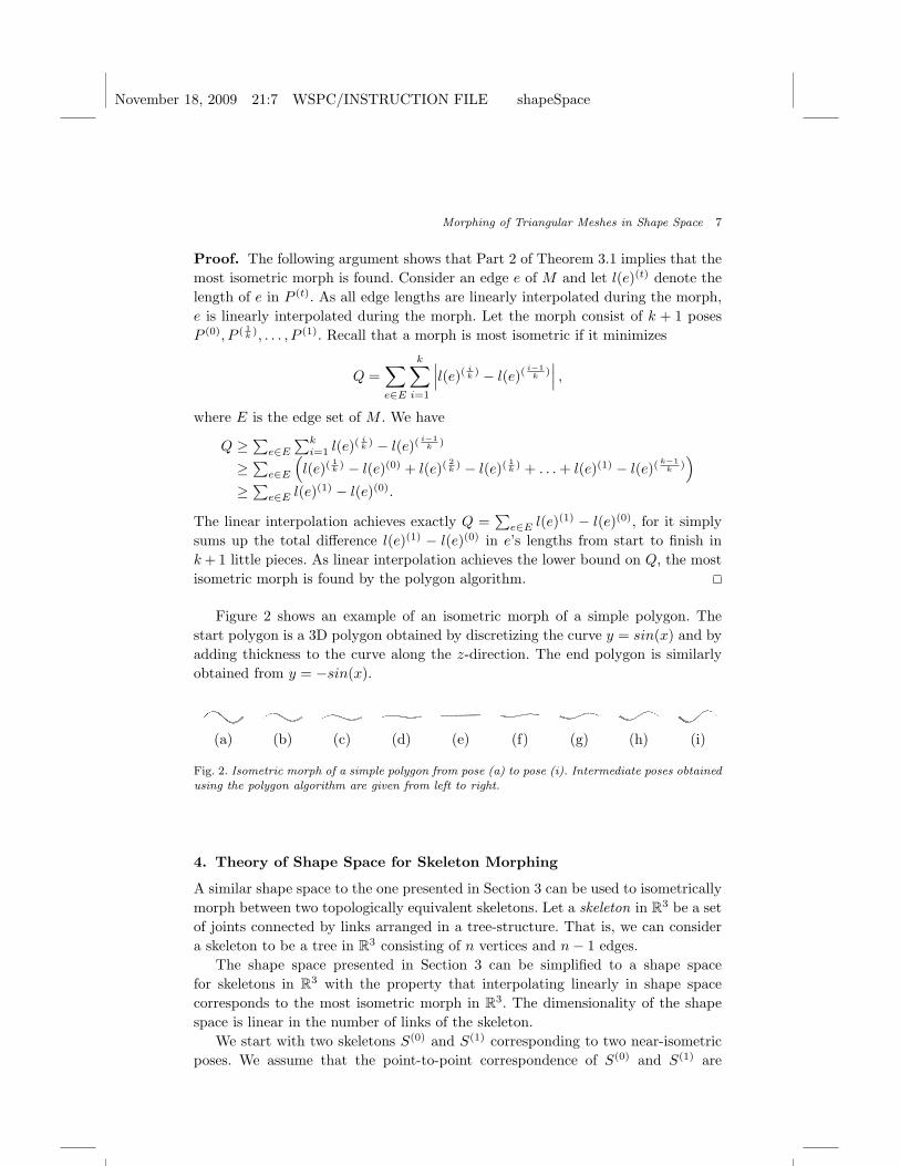
Figure 2 shows an example of an isometric morph of a simple polygon. Thestart polygon is a 3D polygon obtained by discretizing the curve y = sin(x) and byadding thickness to the curve along the z-direction. The end polygon is similarlyobtained from y = −sin(x).

(a) (b) (c) (d) (e) (f) (g) (h) (i)

Fig. 2. Isometric morph of a simple polygon from pose (a) to pose (i). Intermediate poses obtained

using the polygon algorithm are given from left to right.

4. Theory of Shape Space for Skeleton Morphing

A similar shape space to the one presented in Section 3 can be used to isometricallymorph between two topologically equivalent skeletons. Let a skeleton in R3 be a setof joints connected by links arranged in a tree-structure. That is, we can considera skeleton to be a tree in R3 consisting of n vertices and n− 1 edges.

The shape space presented in Section 3 can be simplified to a shape spacefor skeletons in R3 with the property that interpolating linearly in shape spacecorresponds to the most isometric morph in R3. The dimensionality of the shapespace is linear in the number of links of the skeleton.

We start with two skeletons S(0) and S(1) corresponding to two near-isometricposes. We assume that the point-to-point correspondence of S(0) and S(1) are



known. Hence, we know the tree structure T with two sets of ordered vertex coor-dinates V (0) and V (1) in R3. As before, we first find the best rigid alignment of thetwo skeletons.

The skeleton shape space SS is defined in a similar way as S. We assign anarbitrary but fixed root to T and traverse the edges of T in a depth-first order.We assign an arbitrary order to the edges incident on each vertex of T . The first3 coordinates of s correspond to the coordinates of the root in T . The next n − 1coordinates of s are the lengths of the edges in T in depth-first order. The final2(n − 1) coordinates of s describe the unit directions of the edges in sphericalcoordinates in depth-first order. All edges are oriented such that they point awayfrom the root. Note that the shape space S has dimension Θ(n).

Interpolating linearly between points in SS is performed the same way as inter-polating linearly between points in S. Namely, edge lengths are interpolated linearlyand unit directions are interpolated via SLERP. With a technique similar to theproof of Theorem 3.1, we can prove the following theorem. In the proof, we do notneed to consider a dual graph, but we can simply traverse the tree T in depth-firstorder to propagate the information.

Theorem 4.1. Let T be the underlying tree structure of the skeletons S(0) and S(1).The linear interpolation s(t) between s(0) and s(1) in shape space SS for 0 ≤ t ≤ 1has the following properties:

(1) The skeleton S(t) ∈ R3 that corresponds to s(t) ∈ SS is uniquely defined and hasthe underlying tree structure T . We can compute this tree using a depth-firsttraversal of the tree in Θ(n) time.

(2) If S(0) and S(1) are isometric, then S(t) is isometric to S(0) and S(1). If S(0)

and S(1) are not perfectly isometric, then each edge length of S(t) linearly in-terpolates between the corresponding edge lengths of S(0) and S(1).

(3) The coordinates of the vertices of S(t) are a continuous function of t.

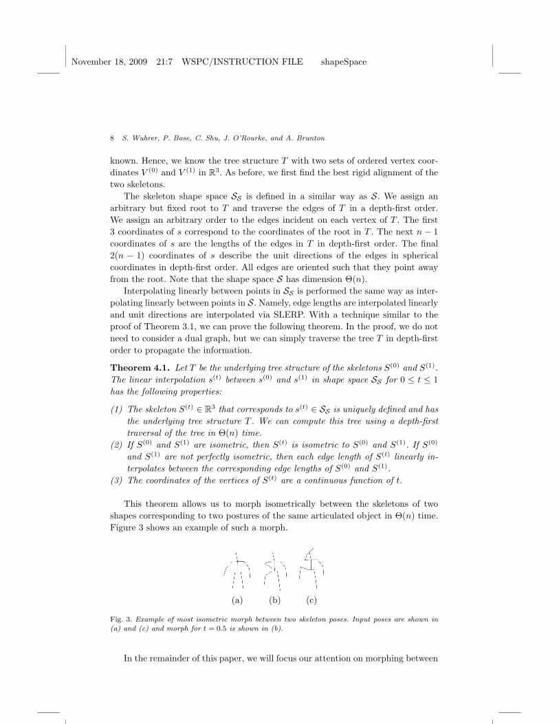
This theorem allows us to morph isometrically between the skeletons of twoshapes corresponding to two postures of the same articulated object in Θ(n) time.Figure 3 shows an example of such a morph.

(a) (b) (c)

Fig. 3. Example of most isometric morph between two skeleton poses. Input poses are shown in

(a) and (c) and morph for t = 0.5 is shown in (b).

In the remainder of this paper, we will focus our attention on morphing between



triangular meshes.

5. Generalization to Triangular Meshes

This section extends the shape space S from Section 3 to arbitrary connected trian-gular meshes. However, we can no longer guarantee the properties of Theorem 3.1,because the dual graph of the triangular mesh M is no longer a tree.

Given two triangular meshes S(0) and S(1) corresponding to two near-isometricposes of the same non-rigid object with known point-to-point correspondence, weknow one mesh structure M with two sets of ordered vertex coordinates V (0) andV (1) in R3.

As before, we can use this information to find the best rigid alignment in R3.We do this before representing the shapes in a shape space. As outlined above, thisalignment has a major influence on the result of the morph.

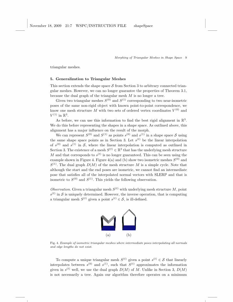
We can represent S(0) and S(1) as points s(0) and s(1) in a shape space S usingthe same shape space points as in Section 3. Let s(t) be the linear interpolationof s(0) and s(1) in S, where the linear interpolation is computed as outlined inSection 3. The existence of a mesh S(t) ∈ R3 that has the underlying mesh structureM and that corresponds to s(t) is no longer guaranteed. This can be seen using theexample shown in Figure 4. Figure 4(a) and (b) show two isometric meshes S(0) andS(1). The dual graph D(M) of the mesh structure M is a simple cycle. Note thatalthough the start and the end poses are isometric, we cannot find an intermediatepose that satisfies all of the interpolated normal vectors with SLERP and that isisometric to S(0) and S(1). This yields the following observation.

Observation. Given a triangular mesh S(t) with underlying mesh structure M , points(t) in S is uniquely determined. However, the inverse operation, that is computinga triangular mesh S(t) given a point s(t) ∈ S, is ill-defined.

(a) (b)

Fig. 4. Example of isometric triangular meshes where intermediate poses interpolating all normalsand edge lengths do not exist.

To compute a unique triangular mesh S(t) given a point s(t) ∈ S that linearlyinterpolates between s(0) and s(1), such that S(t) approximates the informationgiven in s(t) well, we use the dual graph D(M) of M . Unlike in Section 3, D(M)is not necessarily a tree. Again our algorithm therefore operates on a minimum



spanning tree T (M) of D(M). The tree T (M) is computed by assigning a weight toeach arc e of D(M). The weight of e is equal to the difference in dihedral angle of thesupporting planes of the two triangles of M corresponding to the two endpoints ofe. That is, we compute the dihedral angle between the two supporting planes of thetwo triangles of M corresponding to the two endpoints of e for the start pose S(0)

and for the end pose S(1), respectively. The weight of e is then set as the differencebetween those two dihedral angles, which corresponds to the change in dihedralangle during the deformation. The weight can therefore be seen as a measure ofrigidity. The smaller the change in dihedral angle between the two triangles duringthe deformation, the smaller the weight, and the more rigidly the two trianglesmove with respect to each other. As T (M) is a minimum spanning tree, T (M)contains the arcs corresponding to the most rigid components of M , in some sensethe skeleton of the surface.

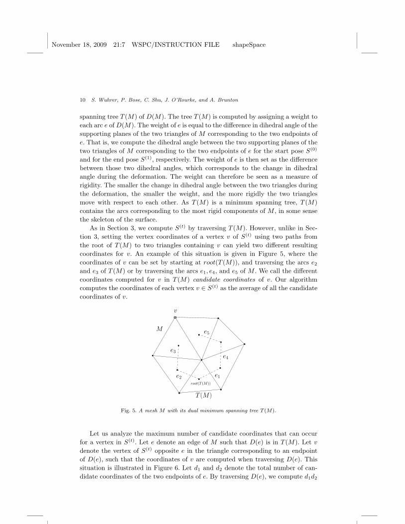
As in Section 3, we compute S(t) by traversing T (M). However, unlike in Sec-tion 3, setting the vertex coordinates of a vertex v of S(t) using two paths fromthe root of T (M) to two triangles containing v can yield two different resultingcoordinates for v. An example of this situation is given in Figure 5, where thecoordinates of v can be set by starting at root(T (M)), and traversing the arcs e2

and e3 of T (M) or by traversing the arcs e1, e4, and e5 of M . We call the differentcoordinates computed for v in T (M) candidate coordinates of v. Our algorithmcomputes the coordinates of each vertex v ∈ S(t) as the average of all the candidatecoordinates of v.

M

T (M)

v

e1

e5

e2

e3e4

root(T (M))

Fig. 5. A mesh M with its dual minimum spanning tree T (M).

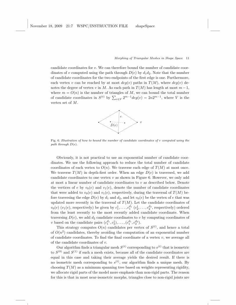
Let us analyze the maximum number of candidate coordinates that can occurfor a vertex in S(t). Let e denote an edge of M such that D(e) is in T (M). Let v

denote the vertex of S(t) opposite e in the triangle corresponding to an endpointof D(e), such that the coordinates of v are computed when traversing D(e). Thissituation is illustrated in Figure 6. Let d1 and d2 denote the total number of can-didate coordinates of the two endpoints of e. By traversing D(e), we compute d1d2



candidate coordinates for v. We can therefore bound the number of candidate coor-dinates of v computed using the path through D(e) by d1d2. Note that the numberof candidate coordinates for the two endpoints of the first edge is one. Furthermore,each vertex v can be reached by at most deg(v) paths in T (M), where deg(v) de-notes the degree of vertex v in M . As each path in T (M) has length at most m−1,where m = O(n) is the number of triangles of M , we can bound the total numberof candidate coordinates in S(t) by

∑v∈V 2m−1deg(v) = 2n2m−1, where V is the

vertex set of M .

e

D(e)v

Fig. 6. Illustration of how to bound the number of candidate coordinates of v computed using thepath through D(e).

Obviously, it is not practical to use an exponential number of candidate coor-dinates. We use the following approach to reduce the total number of candidatecoordinates of each vertex to O(n). We traverse each edge of T (M) at most once.We traverse T (M) in depth-first order. When an edge D(e) is traversed, we addcandidate coordinates to one vertex v as shown in Figure 6. However, we only addat most a linear number of candidate coordinates to v as described below. Denotethe vertices of e by v0(e) and v1(e), denote the number of candidate coordinatesthat were added to v0(e) and v1(e), respectively, during the traversal of T (M) be-fore traversing the edge D(e) by d1 and d2, and let v0(e) be the vertex of e that wasupdated more recently in the traversal of T (M). Let the candidate coordinates ofv0(e) (v1(e), respectively) be given by c1

1, . . . , cd11 (c1

2, . . . , cd22 , respectively) ordered

from the least recently to the most recently added candidate coordinate. Whentraversing D(e), we add d2 candidate coordinates to v by computing coordinates ofv based on the candidate pairs (cd1

1 , c12), . . . , (cd1

1 , cd22 ).

This strategy computes O(n) candidates per vertex of S(t), and hence a totalof O(n2) candidates, thereby avoiding the computation of an exponential numberof candidate coordinates. To find the final coordinate of a vertex v, we average allof the candidate coordinates of v.

Our algorithm finds a triangular mesh S(t) corresponding to s(t) that is isometricto S(0) and S(1) if such a mesh exists, because all of the candidate coordinates areequal in this case and taking their average yields the desired result. If there isno isometric mesh corresponding to s(t), our algorithm finds a unique mesh. Bychoosing T (M) as a minimum spanning tree based on weights representing rigidity,we allocate rigid parts of the model more emphasis than non-rigid parts. The reasonfor this is that in most near-isometric morphs, triangles close to non-rigid joints are



deformed more than triangles in mainly rigid parts of the model. We conclude withthe following.

Proposition 1. Let S(0) and S(1) denote two connected triangular meshes that areisometric to each other and let s(0) and s(1) denote the corresponding shape spacepoints, respectively. We can compute a unique triangular mesh S(t) representingthe information given in the linear interpolation s(t), 0 ≤ t ≤ 1 of s(0) and s(1),in exponential time. We find a triangular mesh S(t) corresponding to s(t) that isisometric to S(0) and S(1) if such a mesh exists.

6. Experiments

The experiments were conducted using an implementation in C++ on an Intel (R)Pentium (R) D with 3.5 GB of RAM. OpenMP was used to improve the efficiencyof the algorithms. To compute the minimum spanning tree T (M), the boost graphlibrary 16 was used.

We use the following data sets in our experiments. The armadillo models arechosen from the AIM@SHAPE repository. a The models contain 331904 triangles.The horse, elephant, and flamingo models were created and used by Sumner et al. 18

The horse models contain 16843 triangles, the cat models contain 14410 triangles,the elephant models contain 84638 triangles, and the flamingo models contain 52895triangles. The head models are from the CAESAR database. 13 The correspondencebetween the two head models was found using the approach by Xi et al. 21 Themodels contain 22091 triangles.

6.1. Results

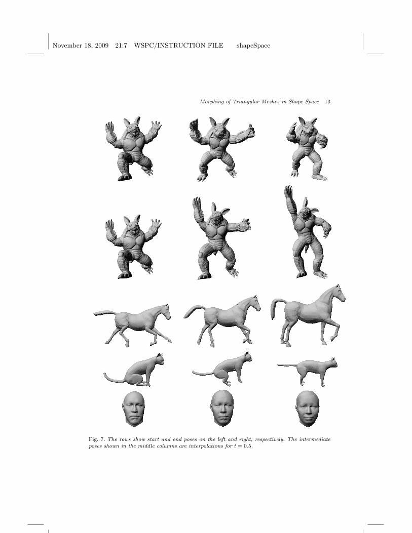
Figure 7 shows a number of morphs. Note that the intermediate poses are visuallypleasing and that most details are preserved during the morph.

ahttp://shapes.aimatshape.net/releases.php



Fig. 7. The rows show start and end poses on the left and right, respectively. The intermediate

poses shown in the middle columns are interpolations for t = 0.5.



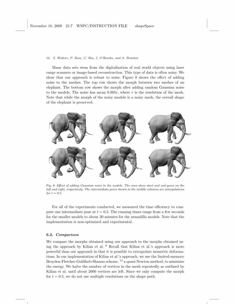
Many data sets stem from the digitalization of real world objects using laserrange scanners or image-based reconstruction. This type of data is often noisy. Weshow that our approach is robust to noise. Figure 8 shows the effect of addingnoise to the meshes. The top row shows the morph between two meshes of anelephant. The bottom row shows the morph after adding random Gaussian noiseto the models. The noise has mean 0.005r, where r is the resolution of the mesh.Note that while the morph of the noisy models is a noisy mesh, the overall shapeof the elephant is preserved.

Fig. 8. Effect of adding Gaussian noise to the models. The rows show start and end poses on theleft and right, respectively. The intermediate poses shown in the middle columns are interpolations

for t = 0.5.

For all of the experiments conducted, we measured the time efficiency to com-pute one intermediate pose at t = 0.5. The running times range from a few secondsfor the smaller models to about 30 minutes for the armadillo models. Note that theimplementation is non-optimized and experimental.

6.2. Comparison

We compare the morphs obtained using our approach to the morphs obtained us-ing the approach by Kilian et al. 8 Recall that Kilian et al.’s approach is morepowerful than our approach in that it is possible to extrapolate isometric deforma-tions. In our implementation of Kilian et al.’s approach, we use the limited-memoryBroyden-Fletcher-Goldfarb-Shanno scheme, 12 a quasi-Newton method, to minimizethe energy. We halve the number of vertices in the mesh repeatedly as outlined byKilian et al. until about 2000 vertices are left. Since we only compute the morphfor t = 0.5, we do not use multiple resolutions on the shape path.



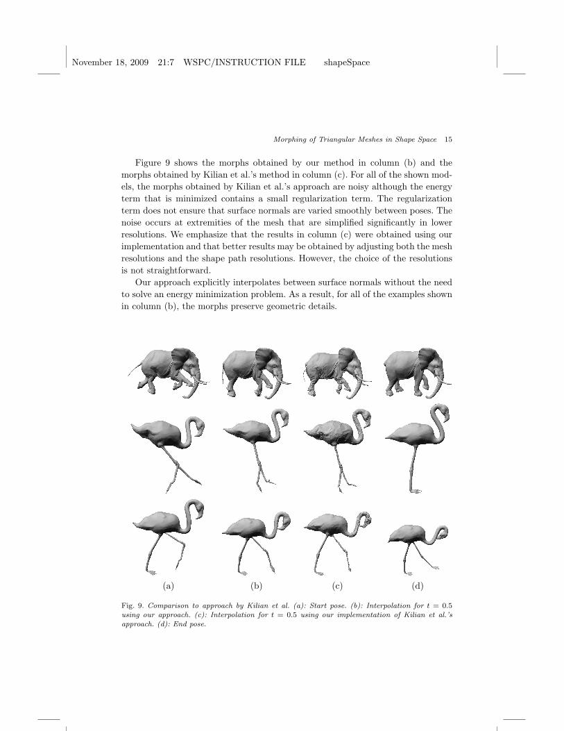
Figure 9 shows the morphs obtained by our method in column (b) and themorphs obtained by Kilian et al.’s method in column (c). For all of the shown mod-els, the morphs obtained by Kilian et al.’s approach are noisy although the energyterm that is minimized contains a small regularization term. The regularizationterm does not ensure that surface normals are varied smoothly between poses. Thenoise occurs at extremities of the mesh that are simplified significantly in lowerresolutions. We emphasize that the results in column (c) were obtained using ourimplementation and that better results may be obtained by adjusting both the meshresolutions and the shape path resolutions. However, the choice of the resolutionsis not straightforward.

Our approach explicitly interpolates between surface normals without the needto solve an energy minimization problem. As a result, for all of the examples shownin column (b), the morphs preserve geometric details.

(a) (b) (c) (d)

Fig. 9. Comparison to approach by Kilian et al. (a): Start pose. (b): Interpolation for t = 0.5

using our approach. (c): Interpolation for t = 0.5 using our implementation of Kilian et al.’s

approach. (d): End pose.



7. Conclusion

We presented an approach to morph efficiently between near-isometric poses oftriangular meshes in a novel shape space. The main advantage of this morphingmethod is that the most isometric morph is always found in linear time when trian-gulated 3D polygons are considered. For general triangular meshes, the approachcannot be proven to find the optimal solution. However, we present an efficientheuristic approach to find a morph for general triangular meshes that does notdepend on solving a non-linear optimization problem.

The presented experimental results demonstrate that the heuristic approachyields visually pleasing results. The running time of the approach can be improvedby employing a multi-resolution scheme.

An interesting direction for future work is to find an efficient way of morphingtriangular meshes while guaranteeing that no self-intersections occur. For polygonsin two dimensions, this problem was solved using an approach based on energyminimization. 6

Acknowledgments

We thank Martin Kilian for sharing his insight on the topic of shape spaces withus. We thank Pengcheng Xi for providing us the data for the head experiment.

References

1. Marc Alexa. Recent advances in mesh morphing. Computer Graphics Forum,21(2):173–196, 2002.

2. Helmut Alt and Leonidas J. Guibas. Discrete Geometric Shapes: Matching, Interpo-lation, and Approximation. In: Jorg-Rudiger Sack and Jorge Urrutia (Editors). Thehandbook of computational geometry, pages 121–153. Elsevier Science, 2000.

3. Prosenjit Bose, Joseph O’Rourke, Chang Shu, and Stefanie Wuhrer. Isometric Morph-ing of Triangular Meshes. In Proceedings of the Canadian Conference on ComputationalGeometry, 2008.

4. Ilya Eckstein, Jean-Philippe Pons, Yiying Tong, C. C. Jay Kuo, and Mathieu Desbrun.Generalized surface flows for mesh processing. In Symposium on Geometry Processing,pages 183–192, 2007.

5. Gene Golub and Charles van Loan. Matrix Computations, Third Edition. The JohnHopkins University Press, 1996.

6. Hayley N. Iben, James F. O’Brien, and Erik D. Demaine. Refolding planar polygons.In Proceedings of the 2006 Symposium on Computational Geometry, pages 71–79, 2006.

7. David Kendall. Shape manifolds, Procrustean metrics and complex projective spaces.Bulletin of the London Mathematical Society, 16:81–121, 1984.

8. Martin Kilian, Niloy J. Mitra, and Helmut Pottmann. Geometric modeling in shapespace. ACM Transactions on Graphics, 26(3), 2007. Proceedings of SIGGRAPH.

9. Vladislav Kraevoy and Alla Sheffer. Mean-Value Geometry Encoding. InternationalJournal of Shape Modeling, 12(1):29–46, 2006.

10. Francis Lazarus and Anne Verroust. Three-dimensional metamorphosis: a survey. TheVisual Computer, 14:373–389, 1998.



11. Yaron Lipman, Olga Sorkine, David Levin, and Daniel Cohen-Or. Linear Rotation-invariant Coordinates for Meshes. ACM Transactions on Graphics, 24(3), 2005. Pro-ceedings of SIGGRAPH.

12. Dong C. Liu and Jorge Nocedal. On the limited memory method for large scaleoptimization. Mathematical Programming, 45:503–528, 1989.

13. Kathleen Robinette, Hans Daanen, and Eric Paquet. The caesar project: A 3-d surfaceanthropometry survey. In 3-D Digital Imaging and Modeling, pages 180–186, 1999.

14. Thomas W. Sederberg, Peisheng Gao, Guojin Wang, and Hong Mu. 2-d shape blend-ing: an intrinsic solution to the vertex path problem. In SIGGRAPH ’93: Proceedingsof the 20th annual conference on Computer graphics and interactive techniques, pages15–18, 1993.

15. Ken Shoemake. Animating rotation with quaternion curves. In SIGGRAPH ’85: Pro-ceedings of the 12th annual conference on Computer graphics and interactive techniques,pages 245–254, 1985.

16. Jeremy G. Siek, Lie-Quan Lee, and Andrew Lumsdaine. The boost graph library: userguide and reference manual. Addison-Wesley Longman Publishing Co., Inc., 2002.

17. Olga Sorkine and Marc Alexa. As-rigid-as-possible surface modeling. In SGP ’07:Proceedings of the fifth Eurographics symposium on Geometry processing, pages 109–116, 2007.

18. Robert W. Sumner and Jovan Popovic. Deformation transfer for triangle meshes.ACM Transactions on Graphics, 23(3):399–405, 2004. Proceedings of SIGGRAPH.

19. Yue Man Sun, Wengping Wang, and Francis Chin. Interpolating polyhedral modelsusing intrinsic shape parameters. The Journal of Visualization and Computer Anima-tion, 8(2):81–96, 1997.

20. Vitaly Surazhsky and Craig Gotsman. Intrinsic morphing of compatible triangula-tions. International Journal of Shape Modeling, 9:191–201, 2003.

21. Pengcheng Xi, Won-Sook Lee, and Chang Shu. Analysis of segmented human bodyscans. In Graphics Interface, 2007.

22. Kun Zhou, Jin Huang, John Snyder, Xinguo Liu, Hujun Bao, Baining Guo, andHeung-Yeung Shum. Large mesh deformation using the volumetric graph laplacian.ACM Transactions on Graphics, 24(3):496–503, 2005.

Documents

Morphing of Triangular Meshes in Shape Spacecs.smith.edu/~jorourke/Papers/shapeSpace.pdf · 2009-11-19 · Morphing of Triangular Meshes in Shape Space 3 shape space corresponds to