Morphing Aerospace Vehicles and Structures (Valasek/Morphing Aerospace Vehicles and Structures) || Hierarchical Control and Planning for Advanced Morphing Systems

P1: TIX/XYZ P2: ABCJWST149-c11 JWST149-Valasek January 11, 2012 19:22 Printer Name: Markono

11Hierarchical Control and Planningfor Advanced Morphing SystemsMrinal Kumar1 and Suman Chakravorty2

1University of Florida, USA2Texas A&M University, USA

11.1 Introduction

This chapter discusses an integrated hierarchical approach to simultaneous planning andcontrol for morphing dynamics. Research in the field of morphing structures has seen recentsurge in interest, especially with the advent of smart structures (e.g. shape memory alloys) thathave made realization of shape changing structures feasible. In addition, the ever increasingdemands on a single structure to accomplish a variety of mission objectives (e.g. an aircraftrequired to conduct both bombing and reconnaissance) has led researchers to explore the fieldof morphing structures in greater detail (Rodriguez 2007; Grant et al. 2006; Hurtado 2006;Wickenheiser and Garcia 2004). Study of morphing dynamics is in general different fromthe study of dynamics of the object itself, and the two may be coupled with each other. Forexample, flight dynamics of an aircraft is traditionally described using a twelve dimensionalstate-space (six translational and six rotational). On the other hand, morphing dynamics of thesame aircraft is described by differential equations that govern reconfiguration of the aircraftfrom one shape (mode of operation) to another. These equations could include dynamicsassociated with smart structures used to build the wings of the reconfigurable aircraft. Theobjective of morphing control then is to find controllers that transform the structure fromone shape to another along a best possible path based on a prescribed metric. In the majorityof cases, true dynamics governing morphing is unknown because of underlying complexity.As a result, model free methods like reinforcement learning (Valasek et al. 2005; Lamptonet al. 2007; Doebbler et al. 2005) (e.g. Q-learning) are popular for control of such systems.Reinforcement learning “learns” the best possible path to the desired goal shape by gatheringinformation about rewards and penalties over numerous Monte Carlo episodes.

Morphing Aerospace Vehicles and Structures, First Edition. Edited by John Valasek.© 2012 John Wiley & Sons, Ltd. Published 2012 by John Wiley & Sons, Ltd.

261


262 Morphing Aerospace Vehicles and Structures

In this chapter, a model-based hierarchical approach for the integrated planning and controlof morphing dynamics is described. All the potential target morphing states to be achievedare contained within the so-called morphing-performance envelope. The objective is to designcontrol laws that transfer the system from one operating point in the envelope to another. Thepresented methodology is an integrated planning and control technique and as such, is closelyrelated to the sequential composition methods (Burridge et al. 1999; Conner 2007; Conneret al. 2007) for deterministic systems and that of hierarchical reinforcement learning (RL) forstochastic systems (Sutton et al. 1999; Parr 1998; Kaebling 1993). In these methods a globalcontrol policy (for stabilization, tracking etc.), is designed by concatenating local policiesthat have smaller (local) domains of operation. The local policies constitute the lower levelof the hierarchy and form the edges of a graph which is superimposed on the performanceenvelope and used as a “highway-system” to traverse inside the envelope. The best path onthe graph is then found between the current and desired points, constituting the higher levelof the hierarchical planning.

11.1.1 Hierarchical Control Philosophy

As briefly mentioned above, the methodology described in this chapter is hierarchical innature, illustrated in Figure 11.1. The starting point is a performance map (shown in top right

Figure 11.1 Schematic of the hierarchical morphing control methodology


Hierarchical Control and Planning for Advanced Morphing Systems 263

section of Figure 11.1), inside which it is desired to move the system from one operatingpoint to another. Each point inside the performance map depicts a morphing trim state wherethe structure is required to operate to fulfill particular mission objectives. Such a map couldpotentially contain a continuum or a discrete set of trim states. In either case, the objective ofhierarchical control is to design controllers at multiple levels to reach a desired trim state fromthe current state. In general, the dynamics of morphing inside the performance map may behybrid in nature, i.e. governed by different dynamical equations in different regions of the map(shown in Figure 11.1). In this chapter, we will consider the special case of uniform dynamicsall across the performance map.

The problem as described above, is to transfer the system from its current operating trimstate to a different morphing trim state on the map, possibly to accomplish a different setof mission objectives. In order to break this problem down, decision-making is divided intotwo levels (hence the hierarchy). The top-level of hierarchy comprises of a connected graphsuperimposed on the performance map. The graph acts like a highway network on whichthe system traverses to reach the vicinity of the target state (Figure 11.1). In other words, thepresented approach ensures that the structure can morph from any state in the performance mapto any other state in some sense of optimality by traversing along the nodes of a connectedgraph on the map. Finding the best route on this highway network to get to the desireddestination constitutes the top level of the hierarchy. The nodes on the graph are connectedto each other bi-directionally (i.e. if it is possible to go from node A to node B, it is alsopossible to go back from node B to A) by means of local controllers. These local controllersconstitute the lower level of the hierarchy. In summary, the hierarchical control works in thefollowing manner: first, a lower level local controller transfers the current morphing-state tothe closest available node on the connected graph. At this point, the top level planner takesover and activates a sequence of lower level controllers to traverse the graph by following apath that minimizes a prescribed cost to arrive at the node closest to the desired trim state.The lower level control takes over again and delivers the morphing-state from the final nodearrived at to the final, desired morphing trim state. The design of such hierarchical controllersmust address the following three questions:

� How is the high level graph containing interconnections of local policies generated?� How are these local policies/controllers designed?� How are the edge costs of the higher level graph, which characterize the higher level

planner, evaluated?

There exists no generic methodology to answer these three questions and most methodsmentioned above provide solutions to particular applications. In this chapter, a method isprovided for automating the solution of the integrated planning/control problem for the classof morphing dynamical systems. Answers to the key questions above are provided by: (1)designing the local policies by leveraging optimal linear controllers that are designed torobustly operate near certain nodes/landmark/trim states of the system; (2) automating thegraph construction on the global domain using these nodes through a novel recursive algorithmsuch that every point in the morphing space is reachable; and (3) using the optimal costsobtained from the local linear designs to specify the edge costs of the graph resulting fromstep 2, to facilitate planning at the higher discrete level.



The end result of hierarchical planning/control design is a hybrid control system (Branicky1995, 1998), or more accurately, a switched linear system in our case (Sun and Ge 2005;Bemporad and Morari 1999; Leonessa et al. 2001). Typically such systems can show verycomplicated behavior even when the component systems are essentially very simple and wellunderstood. Thus, control of such systems is a difficult problem and substantial research inrecent years has concentrated on solving the control problem (Sun and Ge 2005). This chapterpresents a particular instance of such hybrid control systems in which, due to the switchingstrategy that is used between nodes encoded in the discrete higher level graph, the problems ofstability do not arise as in more generic hybrid systems. Essentially, the stability of the localcontrol systems assures the global stability because of the switching strategy that is enforcedon the system. One must also note here the connection to linear parameter varying (LPV)(Leith and Leithead 2000; Rugh and Shamma 2000) and the state dependent Ricatti equation(SDRE) (Cloutier 1997; Hammett et al. 1998) based control of nonlinear systems. In thesemethods, the nonlinear plant is represented in a linear form dependent on an external parameter(as in the case of LPV) or the state of the system (as in SDREs). A stabilizing controller is thenfound by either solving a family of parameter dependent LMIs or a family of state dependentRiccati equations. However, there is no “planning” involved in these controllers, i.e., theydo not tell us where to go next in the context of the morphing problem. Thus, the differencebetween the approach presented here and the above-mentioned methods is the hierarchicalnature of the planner/controller and in particular, the discrete higher level decision-makerin the hierarchical controller while using standard LQ techniques for the design of the lowerlevel controllers.

11.2 Morphing Dynamics and Performance Maps

In this section, mathematical definitions for the various concepts involved in this chapterare presented and the framework for building the hierarchical control strategy is set up.In view of simplicity, we will consider the following deterministic dynamical model formorphing dynamics:

x = f(x, u); x ∈ �N, u ∈ �M (11.1)

where, x depicts the morphing state of the structure. An example is shown in Figure 11.2(a),comprising a triangle with a fixed base. The other two sides change their lengths and aremodeled with spring-damper assemblies. The lengths of the morphing sides along withtheir time derivatives (x1, x2, x1, x2) constitute the morphing state in Equation 11.1 for thisstructure. The vertex is prescribed to move inside the rectangular region shown, which definesthe performance map for this structure. Therefore, the performance map for this structure indefined on the subspace (x1, x2).

In general, the performance map, M of a morphing system is prescribed on a subspace ofthe morphing state in the following manner:

M � {(x1, x2, . . . xn) ⊂ �n}; n ≤ Ne.g., (x1, x2, . . . xn) ∈ [a1, b1] × [a2, b2] × . . . [an, bn]

(11.2)

The problem of optimal morphing control can then be posed in the following manner: For thesystem given by Equation 11.1, design an optimal controller that transfers the system from



PerformanceMap

(a) Two-D morphing triangle

Performance Map Boundary

1.6

1.4

1.2

1

0.8

0.6

0.4

0.2

–1 –0.5 0 0.5 1 1.5 2

0θ1

x2x 1

θ2

θ3

(b) Geometry of the morphing triangle

l

NB

Figure 11.2 A simple morphing structure modeled with nonlinear oscillators

an initial morphing state of xs to a target morphing state, xt , minimizing in the process thefollowing cost function along the path:

J =∫ ∞

0(xTQx + uTRu)dt (11.3)

The above problem can be solved in a suboptimal manner by constructing a connected graph,G on the performance map M, that provides bi-directional access between all points onthe map.

11.2.1 Discretization of Performance Maps via Graphs

The hierarchical approach builds its foundation on a discrete graph that is laid upon theperformance map of the morphing structure. All points on the performance map can bemade accessible from every other point via this graph. In general, there can be many ways ofconstructing this graph. Here, two methods are described: first, a method in which considerablemanual input from the user is required and another which can be completely automated and isamenable to discretation of high dimensional performance maps.

11.2.1.1 Graph Construction: Method 1

This section describes the first of two graph construction techniques described in this chapter.The basic idea is to initialize the graph with a base node and then expand outward by con-structing a nested sequence of envelopes of accessible regions. These envelopes are denotedby �i, i = 1 . . . Q. The last constructed envelope is such that it engulfs the performance map,i.e. M ∈ �Q, thus making almost all points accessible (Figure 11.3). Let us begin with thedefinition of the region of influence (ROI) of a node on the graph.



Performance Map

1 2

34

NB

NB

NB

NB

Ω2

Ω1Ω11

Ω2j

X2j*

*

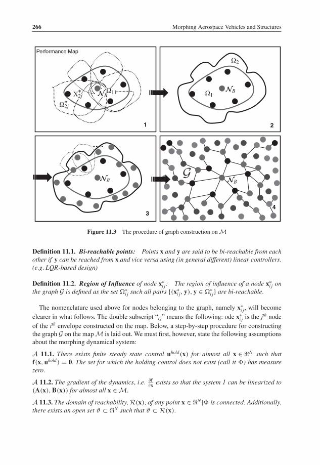
Figure 11.3 The procedure of graph construction on M

Definition 11.1. Bi-reachable points: Points x and y are said to be bi-reachable from eachother if y can be reached from x and vice versa using (in general different) linear controllers.(e.g. LQR-based design)

Definition 11.2. Region of Influence of node x∗i j: The region of influence of a node x∗

i j onthe graph G is defined as the set �∗

i j such all pairs {(x∗i j, y), y ∈ �∗

i j} are bi-reachable.

The nomenclature used above for nodes belonging to the graph, namely x∗i j, will become

clearer in what follows. The double subscript “i j” means the following: ode x∗i j is the jth node

of the ith envelope constructed on the map. Below, a step-by-step procedure for constructingthe graph G on the map M is laid out. We must first, however, state the following assumptionsabout the morphing dynamical system:

A 11.1. There exists finite steady state control uhold(x) for almost all x ∈ �N such thatf(x, uhold) = 0. The set for which the holding control does not exist (call it �) has measurezero.

A 11.2. The gradient of the dynamics, i.e. ∂f∂x exists so that the system 1 can be linearized to

(A(x), B(x)) for almost all x ∈ M.

A 11.3. The domain of reachability, R(x), of any point x ∈ �N |� is connected. Additionally,there exists an open set ϑ ⊂ �N such that ϑ ⊂ R(x).



The set � represents points that are not reachable in the morphing system 1. This chapteris only concerned with systems for which this set has zero measure and thus excluded fromanalysis. Assumption 11.1 can be relaxed in practice to perform the analysis for only thereachable points inside M. Assumption 11.2 restricts the realm of the described approachto those systems for which a linearized representation can be found for almost all points(excluding sets of zero measure) inside the performance map. Assumption 11.3 is essential forthe present approach for determining regions of influence. Note that R(x) is different fromROI(x). From definition 11.2, it is clear that ROI(x) ⊂ R(x). A parametric-sweep approachwill be utilized for determining ROI(x) which would formally work for systems satisfyingassumption 11.3.

Given the validity of the above assumptions, the following result can be stated:

Theorem 11.1. For the morphing system 1 with a continuous performance map, M, givenassumptions 2.1, 2.2 and 2.3, a connected graph, G, can be constructed on M with a finitenumber of nodes, {x∗

i j} (∑

i, j = P) such that all points yt ∈ M can be reached from any otherpoint ys ∈ M to within a specified tolerance, i.e., ‖x(t = ∞, ys) − yt‖ ≤ ε by traversing G.

The following steps outline the procedure for graph construction and also serve as a con-structive proof for the above theorem. As mentioned previously, the basic idea is to constructa sequence of expanding envelopes, �i, i = 1 . . . Q that eventually engulfs the map M, i.e.M ∈ �Q. Figure 11.3 illustrates this process.

1. Graph construction begins with the base node. This node represents the most likely trim-state of the morphing dynamics, and is denoted by NB in Figure 11.3. For the morphingtriangle, this represents the equilateral-triangle configuration. (see Figure 11.2(b)) Denotethis node by x∗

i j = x∗11.

2. Estimate the region of influence of this node. This is done by performing a parametricsweep of the boundary of the performance map and determining the farthest point that isbi-reachable for each value of the parameter set. (see definition 11.1 of bi-reachability) Aparametric representation is thus obtained for the boundary of the region of reachabilityby joining the farthest bi-reachable points. Figure 11.4(a) illustrates this process for atwo-dimensional map. In this figure, a rough estimate of the region of influence of theshown node has been obtained by utilizing a single parameter (θ ) sweep with 6 points.The farthest points bi-reachable from the node for each value of the sweeping parameterhave been joined to obtain the region of influence. In general, an N dimensional performancemap would require a parameter set of (N − 1) independent parameters. The farthest pointfor any particular value of the parameter set is estimated by the process of successive LQR(Figure 11.4(b)). In this process, progressively closer points are chosen (in Figure 11.4(b)by bisection) until a bi-reachable point is obtained. Note that this approach requires thevalidity of assumption 11.3 for an accurate estimate of ROI(x∗

i j). The sweeping processresults in the boundary of ROI(x∗

i j), namely, �∗i j. Also note that ROI(x∗

i j) is referred to as�∗

i j. The first in the sequence of envelopes, �1 is simply the ROI of the base node, i.e.�1 = �∗

i j.3. Discretize �∗

i j by placing nodes as shown in Figure 11.3. These nodes form the base forconstructing the next envelope and we denote them by x∗

2 j, where j = 1, 2, . . . R. (numberof nodes used to discretize �1)



xx

x

xx

x

θ1

θ2θ3

θ4

θ5

θ6

(a) Parametric sweep on a two dimensional performance map

×

×

+initial state

desiredtarget state

×

×

+×

initial state bi-reachable target state

new target state ××

×××

++++++initial state

desiredtarget state

××

×××

++++++××

initial state et bi-reachable targeea×statee

new target gstatestate

(b) Successive LQR approach to determine bi-reachable pairs

Figure 11.4 Determining the region of influence for a node on the graph

4. Determine the ROI’s for x∗2 j, i.e. �∗

2 j.5. Determine the new envelope as �2 = ∪R

i=1�∗2 j ∪ �1. Denote boundary (�2) = �2. Note

from Figure 11.3 that the construction results in a sequence of nested envelopes �2 ⊂ �1.The process is repeated until Q envelopes are generated so that the final envelope engulfs theperformance map: M ⊂ �Q. The entire set of nodes used in this construction constitutesthe graph and is seen in Figure 11.3.

Step 3 in the above algorithm can be manually intensive and require input from the user.This becomes increasingly difficult as the dimensionality of the performance map grows.For high dimensional scenarios, an alternate technique is therefore desired, one which maybe fully automated. The section below describes one such method, based on the use ofpseudo-random numbers.

11.2.1.2 Graph Construction Method 2: Pseudo Random Graphs

This section describes an alternate method of graph construction based on pseudo randomnumbers. Dimensionality of the performance map can become a serious issue in the graphconstruction method described in the previous section. In dimensions three and higher, it is verydifficult to manually place nodes to discretize the envelopes in step 3. Instead, pseudo randomsampling can be used to construct a connected graph to cover the entire performance mapefficiently with no manual input. Pseudo random numbers have been widely used to samplereal spaces for the purpose of numerical integration. They are generated using an algorithm,with the particular algorithm used determining the variety of psuedo random numbers obtained,e.g. Halton pseudo random numbers, Sobol numbers, Fauvre numbers, etc. A pseudo randomsequence, even though algorithmically generated, gives the appearance of having a uniformrandom distribution over the sampled region (hence the qualification “pseudo”). The actualseparation of the sample from a true uniform distribution is typically quantified using certaindiscrepancy parameters (Niederreiter 1992). In the present context, they can be utilized to



(a) Pseudo random numbers in two-dimensional space (b) Pseudo random numbers in three-dimensional space

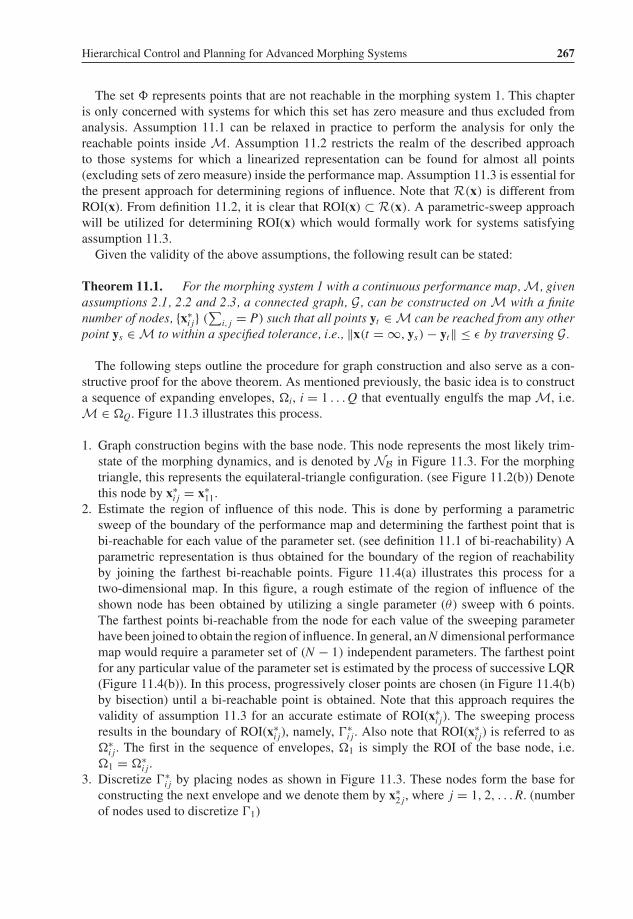
Figure 11.5 Examples of pseudo random numbers (halton sequence) in two- and three-dimensionalspaces

uniformly distribute nodes on the performance map which can be connected to construct thegraph of interest. Examples of pseudo random distributions (Halton sequence) in two and threedimensions are shown in Figure 11.5. It is also important to note that it is very easy to locallysample pseudo random points if the density in a certain area is low. Additionally, it is alsoeasy to generate high dimensional pseudo random numbers, thus making them suitable to highdimensional performance maps. The following steps briefly outline the graph constructionprocedure:

1. Let the dimensionality of the performance map be n, i.e. M ⊂ �n. Generate a total of P0 ndimensional pseudo random numbers xi ∈ M, i = 1, . . . P0. The number P0 is the startingguess for the total number of nodes in the graph G. The nodes xi, i = 1, . . . P0 form theinitial estimate of the graph (currently not connected).

2. For each i = 1, 2, . . . , P, do the following(a) Consider a n dimensional box Mo ⊂ M whose volume is a small percentage (perhaps

5%) of the volume of M. Translate the box such that the current node (xi) is itscentroid. Find all the nodes lying inside Mo, labeling them xi j, j = 1, 2, . . . Qi, thepotential neighbors of xi.

(b) Attempt to design controllers (the type of controller is up to the user, e.g. LQR) totransfer the system from xi to xi j and back from xi j to xi. In other words, determinewhich points out of xi j are bi-directionally connected to xi. If this set is not empty,move to the next point, i.e. i → i + 1 and go back to step 2, otherwise go to the nextstep.

(c) (If node xi does not have any bi-directional neighbors.) Resample the box Mo with asmall number of pseudo random points to increase node density and re-do step 2(b).Record the bi-directional neighbors for node xi.

Given the validity of assumptions 11.1–11.3, the above steps guarantee the construction of aconnected graph on M such that all points inside it are reachable from every other point in



M. Note that the above sequence of steps does not require any manual input and is suitablefor high dimensional performance maps.

11.2.2 Planning on Morphing Graphs

In this section, the top level of the hierarchical control strategy is described. Once is graphis constructed, it is desired to know the best routes on it from any given node to any othernode. Depending on the number of nodes on the graph, this search may be performed onlineor may need to be offline and stored away for future access. There are numerous techniquesin the literature that may be used to search for optimal paths on a graph. Here, we describe atwo-level A∗ algorithm for this purpose. Note that the objective here is not to find a path ofshortest “distance,” but one of least cost which is defined based on the design of the lower levelcontrollers used to connect the nodes on the graph with each other. This cost may be relatedto a time parameter or fuel expense or something else. The problem therefore is to find a pathconnecting two nodes on the graph along which this particular cost of interest is minimized.

Standard A∗ algorithms work well for path-planning applications where it is needed to finda minimum-distance path between any two points on the graph. The performance of the A∗

algorithm hinges on a heuristic function that estimates the cost-to-go from the current nodeto the destination node. In order to guarantee convergence to the optimal path, it is required(though not always) that the heuristic function under-estimate the cost-to-go from the currentnode. Such a heuristic function is said to be admissible. For a problem that seeks to findthe minimum distance path, it is easy to find an admissible heuristic function, simply as theEuclidean distance between the concerned points. In the current application however, it isrequired to find an optimal path based on the metric given in Equation 11.3 (or any otherprescribed cost on the basis of which the local, low level controllers are based). We note that itis extremely difficult to find an admissible heuristic function for such an arbitrary cost function.The two-level A∗ search described below takes care of this problem and generates a feasibleheuristic function. Such a function ensures convergence, but not necessarily to the optimalpath because it does not always provide an under-estimate of the cost-to-go. The two-level A∗

is described in the next section.

11.2.2.1 Two-Level A∗

Problem statement: Given graph G, find the optimal path from node xo to x f . Two-levelalgorithm:

� Let OL be the current open-list of the search. Open-list is the collection of points that havealready been visited but not expanded (explored) yet.

� Define auxiliary heuristic cost, h(x) = ‖x f − x‖. This is simply the Euclidean distance costfor which the standard A∗ algorithm works well.

� For each xk ∈ OL, run the A∗ algorithm to determine the optimal path from xk to x f using theauxiliary heuristic function, h(x). Let the obtained path for xk bePk = {xk, xk1, xk2, . . . , x f }.

� Determine the heuristic cost for the node xk as:

h(xk) =∫Pk

(xTQx + uTRu)dt (11.4)



� Using h(xk) as the heuristic function, determine the lowest cost node to remove from theopen-list and add to the closed-list, CL.

� Continue until x f ∈ CL.

The above algorithm results in a sequence of nodes connecting xo to x f which may be storedaway for each such pair in the graph for future reference.

11.3 Application to Advanced Morphing Structures

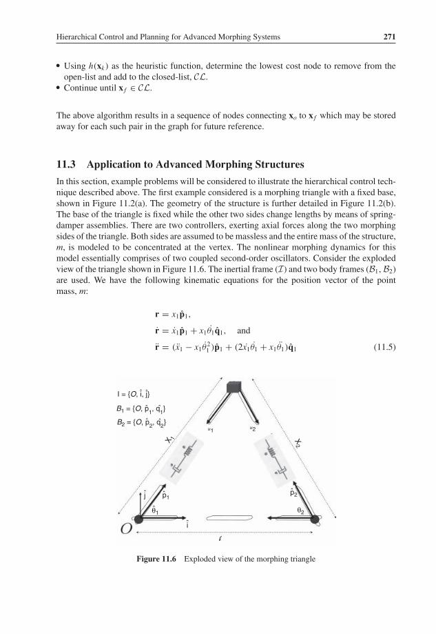
In this section, example problems will be considered to illustrate the hierarchical control tech-nique described above. The first example considered is a morphing triangle with a fixed base,shown in Figure 11.2(a). The geometry of the structure is further detailed in Figure 11.2(b).The base of the triangle is fixed while the other two sides change lengths by means of spring-damper assemblies. There are two controllers, exerting axial forces along the two morphingsides of the triangle. Both sides are assumed to be massless and the entire mass of the structure,m, is modeled to be concentrated at the vertex. The nonlinear morphing dynamics for thismodel essentially comprises of two coupled second-order oscillators. Consider the explodedview of the triangle shown in Figure 11.6. The inertial frame (I) and two body frames (B1,B2)are used. We have the following kinematic equations for the position vector of the pointmass, m:

r = x1p1,

r = x1p1 + x1θ1q1, and

r = (x1 − x1θ21 )p1 + (2x1θ1 + x1θ1)q1 (11.5)

B1 = {O, p1, q

1}

B2 = {O, p2, q

2}

X 1 X2

ˆ

p1ˆ p2ˆ

θ1ˆ θ2

ˆ

ˆˆ

j

i

I = {O, i, j}ˆ ˆ

u1u2

Figure 11.6 Exploded view of the morphing triangle



The spring/damper forces and the controls can be expressed as:

F = [k1(x1) + c1(x1, x1)︸︷︷︸f1

+u1](−p1) + [k2(x2) + c2(x2, x2)︸︷︷︸f2

+u2](− cos θ3p1 − sin θ3q1)

(11.6)Consideration of geometrical constraints for the triangular structure leads to following theequations relating the angular rates, θ1 and θ1 to the morphing states:

θ1 = 1

lx1 sin θ1(x2x2 + lx1 cos θ1 − x1x1)

θ1 = − 1

x1

[x1θ

21 − f1 + u1 + ( f2 + u2) cos θ3

m

](11.7)

We are thus lead to the equations for morphing-dynamics in state-space form:

x1 = x3

x2 = x4

x3 = x1θ21 + 1

m[ f1 + u1 + ( f2 + u2) cos θ3]

x4 = 1

x2[x2

1 − x22 + (x1 − l cos θ1)x3 + 2lx1θ1 sin θ1 + lx1θ

21 cos θ1 + lx1θ1 sin θ1] (11.8)

The various trigonometric functions appearing in Equations 11.7 and 11.8 can be obtained eas-ily in terms of the states, x1 and x2. Finally, the nonlinear spring-damper forces can be modeledwith the following constitutive equations: (there can be numerous other constitutive laws)

f1 = k1l(x1 − l) + k1nl(x1 − l)3 + c1l x1 + c1nlx1θ1

f2 = k2l(x2 − l) + k2nl(x2 − l)3 + c2l x2 + c2nlx2θ2 (11.9)

In order to implement the successive LQR algorithm, it is required to linearize the dynamics(Equation 11.8) about the current steady state condition (trim). The following are thelinearized equations of motion for the morphing triangle about a trim state, xss: (all subscripts‘ss’ denote steady state conditions)

δx1 = δx3

δx2 = δx4

δx3 = − 1

m[δ f1 + δu1 + cos θ3ss(δ f2 + δu2) − sin θ3ss( f2ss + u2ss)δθ3]

δx4 = x1ss − l cos θ1ss

x2ssδx3 + l

x1ss

x2sssin θ1ssδθ1 (11.10)

where, θ3 = π − (θ1 + θ2). The linearized equations for the angles and their rates used aboveare given by:



δθ1 = −1

lx1ss sin θ1ss[(x1ss − l cos θ1ss)δx1 − x2ssδx2]

δθ2 = −1

lx2ss sin θ2ss[(x2ss − l cos θ2ss)δx2 − x1ssδx1], δθ3 = −(δθ1 + δθ2)

δθ1 = 1

lx1ss sin θ1ss[x2ssδx2 + (l cos θ1ss − x1ss)]δx3

δθ1 = −1

mx1ss[( f2ss + u2ss) cos θ3ssδθ3 + sin θ3ss(δ f2 + δu2)] (11.11)

It is easy to obtain the departure values for the forces, i.e., δ f1 and δ f2 in terms of themorphing-states from Equation 11.9. Since it is required to transfer the morphing-state fromone trim to another, the problem at hand is one of non-zero set point regulation; wherein, itis desired to obtain a non-zero steady-state value for the departure state. We will now look atthat problem. The linearized equations above can be assembled into linear state-space formas δx = Aδx + Bδu. Let the desired steady-state value of the departure motion be δx∗. Thenwe perform the following transformation of coordinates:

δx � δx − δx∗

δu � δu − δu∗ (11.12)

The steady-state condition requires that: Aδx∗ + Bδu∗ = 0. The transformed equations thenreduce to:

δ ˙x = Aδx + Bδu − Aδx∗ − Bδu∗ = Aδx + Bδu (11.13)

Note that the above transformation reduces the problem to the standard regulator problem,in which it is desired to obtain limt→∞ δx = 0. The standard LQR solution to this problem isgiven by δu = −Kδx. It remains to find δu∗. To this end, we exploit the steady-state conditionand note that:

δx∗ =

⎧⎪⎪⎨⎪⎪⎩

δx∗1

δx∗2

00

⎫⎪⎪⎬⎪⎪⎭ ; δu∗ =

{δu∗

1

δu∗2

}; A =

⎡⎢⎢⎣

0 0 1 00 0 0 1× × × ×× × × ×

⎤⎥⎥⎦ ; B =

⎡⎢⎢⎣

0 00 0× ×× ×

⎤⎥⎥⎦ ;

∴ Aδx∗ + Bδu∗ = 0 ⇒

⎧⎪⎪⎨⎪⎪⎩

00c1

c2

⎫⎪⎪⎬⎪⎪⎭ +

⎧⎪⎪⎪⎨⎪⎪⎪⎩

00[

b1 b2

b3 b4

] {δu∗

1

δu∗2

}⎫⎪⎪⎪⎬⎪⎪⎪⎭ =

⎧⎪⎪⎨⎪⎪⎩

0000

⎫⎪⎪⎬⎪⎪⎭ (11.14)

It is easy to obtain a solution for the steady-state control δu∗ from the above equation.

11.3.1 Morphing Graph Construction

The graph construction for the morphing triangle begins with the base node shown in Fig-ure 11.2(b) which represents the equilateral triangle configuration.As outlined in the algorithm



(a) Region of influence of the base node (Ω11) and itsdiscretized boundary (Γ11). Γ1 = Γ11

(b) Region of influence of x*2j, j = 1, 2, ...., 34

(c) Nested envelopes that engulf the performance map (d) Obtained least cost path using the A* search algorithm

Figure 11.7 Graph construction and search for the morphing triangle

above, starting with the base node, we construct a graph that grows outward, eventually en-gulfing the performance map defined by the limits on the movement of the vertex. Figure 11.7depicts this process. In Figure 11.7(a), the domain of the influence of the base node is shown.By construction, all points inside this region are accessible from the base node, and vice versa;i.e., the base node is bi-reachable with all points inside this region. Following the nomen-clature in the algorithm, the depicted region is �∗

11 = �1. The shown boundary is �∗11 = �1.

Figure 11.7(a) shows the discretization of �1 using 34 points (= x∗2 j). The domains of influence

for these nodes (= �∗2 j) are shown in Figure 11.7(b). Figure 11.7(c). shows that continuing

with this process results in a set of expanding nested envelopes which eventually engulf M.(M ⊂ �11) Figure 11.7(d) shows all the nodes that comprise the graph G on M. Also on thisfigure is shown the solved problem of finding an optimal path between two nodes. A two-levelA∗ algorithm was used to find this path.

A sample solution of the above algorithm is shown in Figure 11.7(d). Note that the heuristiccost evaluated for xk in Equation 11.4 over the minimum distance path, P , is not necessarily an



(a) The Kagomé lattice pattern (b) A Kagomé basket (source: Wikipedia)

Figure 11.8 The Kagome lattice

underestimate of the actual cost-to-go from xk. Therefore, h(x) is not admissible, only feasible.In the authors’ experience, the results obtained from this approach have been extremely good,with no convergence issues.

11.3.2 Introduction to the Kagome Truss

In this section, advanced morphing structural concepts using the Kagome truss are brieflydiscussed. Kagome, which literally means “a basket with eyes,” (“kago” = basket, “me” =eyes) is a traditional Japanese weaving pattern, shown in Figure 11.8. Note from the highlightednodes in Figure 11.8(a) that for any node on the lattice, there are four neighboring nodes.

The first paper on this subject was published in 1951 by Japanese physicist Itiro Syozi.There have been numerous papers written on the Kagome lattice, particularly in the structurescommunity. The structure has emerged as being capable of bearing large passive loads at anextremely low weight (Hutchinson et al. 2003; dos Santos e Lucato et al. 2004). The use of theassociated Kagome truss has not been fully explored in the aerospace community. The authorsbelieve that the superior load bearing capacity of the Kagome truss can be utilized to greatadvantage for problems in aerospace engineering. In this section, a morphing structure basedon the Kagome truss from dos Santos e Lucato et al. (2004) is adapted and used to illustrate thethe hierarchical control methodology. Figure 11.9(a) illustrates a morphing structure mountedon a Kagome truss. The Kagome truss (marked with broken lines) constitutes the base of thestructure and comprises of morphing elements. A tetrahedral core (shown with solid lines) ismounted on top of the base and consists of non-morphing elements. In other words, the legsof the tetrahedral core are fixed in length. A face-plate (shown as a shaded surface atop thetetrahedral core) is attached to the core at the vertices of the tetrahedra, and it forms the outersurface of the morphing structure. This could be the outer surface of a wing. The desired shapeof the face-plate is obtained by morphing the Kagome truss (at the base) alone. Changing thelengths of the sides of the Kagome truss causes the vertices of the various tetrahedra to moveup or down, in turn moving the face-plate to the desired shape. Such a structure provides greatflexibility and a wide range of attainable shapes. Figure 11.10 shows a possible wing morphingapplication using the Kagome truss structure, wherein the top-surface of a symmetric wing ismorphed into a wing with large camber.



1.2

1

0.8

0.6

6

5

4

3

2

1

00 1 2 3 4 5 6 7 8 9

0.4

0.2

06

4

2

06 5 4 3 2 1 0

(a) A morphing structure based on the Kagomé truss (b) Location of actuators in a fully morphing Kagomé truss

Figure 11.9 Details of the Kagome truss

A great advantage of using the Kagome truss to morph the face-plate is that the underlyingmorphing control problem is a two-dimensional structure (the Kagome truss). All we need is atransformation describing the lengths of the Kagome truss elements as a function of the heightsof the various tetrahedral vertices. Figure 11.11 illustrates the details of such a transformation.Consider an isolated element of the Kagome base shown in Figure 11.11(a). All the elementsof the tetrahedral core are assumed to have the same length. It is desired that the vertex of thelower tetrahedron be at the position marked by the diamond. Top and side views are shown.The problem then is to determine what the new lengths of the triangle should be in order forthe vertex to be located at the desired location. It turns out that this problem has a non-uniquesolution, shown in Figure 11.11(b). The locus of solutions is the circle drawn by the individuallegs of the tetrahedron on the plane of the Kagome truss. Since all three legs are assumedto have the same lengths, they all describe the same circle, centered at the projection of thedesired vertex location on the base plane. The solution then is to simply move the verticesof the base triangle onto a point on the circle, as shown in Figure 11.11(b), leading to thenew configuration on the base triangle (shown with broken lines). The non-uniqueness comesform the fact that the user the free to move the base triangle vertices to any point on this

(a) Top surface of a symmetric wing (b) Top surface of a cambered wing

Figure 11.10 Wing morphing using the face-plate atop a Kagome truss assembly



3.5

1

0.8

0.6

0.4

0.2

0

–2 –1.5 –1–0.5 0 0.5 1 1.5 2 2.5 3 3.5

3

1

0

–1

–2

2

3

2.5

2

1.5

1

0.5

0

–0.5

–1

–1.5

–2–2 –1.5–1–0.5 0 0.5 1 1.5 2 2.5 3 3.5

3.5

3

3.5

2

1.5

1

0.5

0

–0.5

–1

–1.5

–2–2 –1.5 –1 –0.5 0 0.5 1 1.5 2 2.5 3 3.5

(a) Desired location of the tetrahefron’s vertex (b) A non-unique solution to the transformation problem

Figure 11.11 The problem of transformation of the tetrahedron-vertex location to the configuration ofthe base triangle

circle. A possible strategy could be to move the vertices to the closest respective points on thecircle. This then becomes the equivalent morphing problem to obtain the desired position ofthe vertex. Note that in case the legs of the tetrahedron are of different lengths, there would bethree concentric circles of different radii and it would be required to move the three verticesof the triangle to the appropriate circles.

11.3.3 Examples of Morphing with the Kagome Truss

In this section, morphing examples are considered for the Kagome truss structure. The firstinvolves a constrained structure in which the morphing elements of the Kagome base are thesame as the morphing triangle shown in Figure 11.6 with fixed bases. A single Kagome unit isextracted and the three triangular shapes shown in Figure 11.12 morph independently of eachother. The desired shape of the face-plate is shown in Figure 11.12(b). Only the final resultis shown here, including the final shape of the individual triangles. More complex morphingshapes can be achieved with the Kagome truss if all three sides of the triangular units areallowed to morph. In this chapter, only an initial description of this problem is given andmore detailed analysis is currently under investigation. Figure 11.9(b) illustrates the location

(a) Current and desired shapes of the face-plate

1

0.8

0.6

0.4

0.2

0

3 2 1 0 –1 –2 –1 02 3

Desired configuration

Base configuration

1

4 3.5

3

2.5

2

1.5

10.5

0–0.5

–1

–1.5–2

2

3

(b) The final obtained configuration of the Kagomé base truss for the desiredshape of the face-plate

1

0

–1

–2–2 –1.5 –1 –0.5 0 0.5 1 1.5 2 2.5 3 –1.5–2 –1 –0.5 0 0.5 1 1.5 2 2.5 3 3.5

Figure 11.12 An example morphing problem using the Kagome truss



(a) Current and desired shapes of the face-plate

(c) Current and desired shapes of the face-plate

(b) The final obtained configuration of the Kagomé basetruss for the desired shape of the face-plate

(b) The final obtained configuration of the Kagomé basetruss for the desired shape of the face-plate

14 1

12

10

8

6

4

2

00 2 4 6 8 10 12 14 16 18

14

0.6

0.8

0.4

0.2

0.0

20

15

10

5

14

14

1

0.8

0.6

0.4

0.2

0

12 10 8 6 2 0 –20

0

10

2

4

12 10 8 6 4 2 0

12

10

8

6

4

2

0

–2–2 0 2 4 6 8 10 14 16 1812

Figure 11.13 An example morphing problem using the Kagome truss

of actuators in an assembly where all three sides of the triangular elements are allowed tomove. This figure depicts a “three-channel” Kagome truss with four hexagonal units in thelowest channel. In a more general structure, if the number of channels is c and the number ofhexagonal units in the lowest channel is h, the total number of actuators is: 3

2 c(2h − c + 3).Of course, the number of actuated triangles is one-third of this number, as is clearly visiblefrom Figure 11.9(b).

The dynamic modeling of this scenario is more complex because it involves all hexagonalunits of the Kagome base moving together. The end result is a very high dimensional (possiblyin the hundreds) morphing state space and equivalently high dimensional performance map.The problem can be greatly simplified if the structure is assumed to morph one hexagonalunit at a time, locking down the remaining Kagome base until only the activated unit attainsits target shape. Under this assumption, the dimensionality of the morphing state would besix, which despite being still a sizeable value can be easily handled using the pseudo randomgraph construction technique described in Section 11.2.1.

An example of a fully morphing Kagome truss is shown in Figure 11.13. The base config-uration is a flat face-plate, with the Kagome base composed of 7 (= c) channels of hexagonal



Kagome units and the lowest channel with 8 (= h) hexagonal units. This counts for a total of126 actuators (a very large number!). The morphing problem is to convert the flat face-plateto the quadratic shape shown in Figure 11.13(d). The resulting morphed shape of the Kagomebase is shown in Figure 11.13(c). A comparison with the flat face-plate truss configuration isalso shown in this figure, using dotted lines. Note that this figure only represents a geometricalsolution to the described problem using the rules of inverse transform described in the abovesection and Figure 11.11. The development of dynamical equations and related control lawsbased on the hierarchical methodology for this type of structure is currently under investigationand will be the topic of a future article.

In summary, the authors believe that the above-described morphing structure based on theKagome truss holds great promise for building morphing structures for aircraft. There remainsa lot of be studied yet and the current work exhibits initial promise. Some challenges includeaccurate modeling of the morphing elements of the Kagome base, determination of the densityof the tetrahedral core, dynamic structural analysis of the structure and aeroelastic behavior ifused in a wing-application among several others.

11.4 Conclusion

In this chapter, a hierarchical, model-based approach for optimal control of morphing dynamicswas presented. It was shown that a connected graph can be imposed on the performance mapof a morphing structure, making all points on the map accessible from every other point viathe graph. Two techniques for graph construction were presented, one requiring considerablemanual input, and the other suitable for high dimensional applications using pseudo randomsequences. The control laws for lower level control were designed using non-zero set pointLQR. An example problem based on a morphing triangle with a fixed base was presented. Arudimentary description of morphing problems using the Kagome truss was also given. It isproposed that a morphing structure based on the Kagome turss can be used to great advantagein the aerospace community for morphing aircraft applications.

ReferencesBemporad A and Morari M 1999 Control of systems integrating logic, dynamics and constraints. Automatica, 35(3):

407–427.Branicky MS 1995 Studies in hybrid systems: modeling, analysis and control, PhD thesis. Dept. of Electrical

Engineering and Computer Science, MIT.Branicky MS 1998 Multiple Lyapunov functions and other analysis tools for switched and hybrid systems. IEEE

Transactions on Automatic Control, 43(4): 475–482.5Burridge RR, Rizzi, AA and Koditschek D 1999 Sequential composition of dynamically dexterous robot behaviour.

International Journal of Robotic Research, 18(6): 535–555.Cloutier JR 1997 State dependent Riccati equation techniques. In Proceedings of the American Control Conference,

Albuquerque, NM, June, pp. 932–936.Conner DC 2007 Integrating planning and control for constrained dynamical systems, PhD thesis. Robotics Institute,

Carnegie Mellon University, Pittsburgh, PA.Conner DC, Kress-Gazit H, Choset H, Rizzi A, and Pappas GJ 2007 Valet parking without a valet. In Proceedings of

the 2007 IEEE/RSJ International Conference on Intelligent Robots and Systems, San Diego, October.Doebbler J, Tandale M, Valasek J, and Meade A 2005 Improved adaptive-reinforcement learning control for morphing

unmanned air vehicles. AIAA Paper 2005–7159. Arlington, TX, USA, 26–29 Sept.dos Santos e Lucato SL, Wang J, Maxwell P, McMeeking RM, and Evans AG 2004 Design and demonstration of a

high authority shape morphing structure. International Journal of Solids and Structures, 41: 3521–3543.



Grant DT, Abdulrahim M, and Lind R 2006 Flight dynamics of a morphing aircraft utilizing independent multiple-jointwing sweep. AIAA Paper 20066505. Keystone, CO, USA, 21–24 Aug.

Hammett KD, Hall CD, and Ridgely DB 1998 Controllability issues in nonlinear state dependent Riccati equationcontrol. Journal of Guidance Control and Dynamics, 21(5).

Hurtado JE 2006 Dynamic shape control of a morphing airfoil using spatially distributed actuators. AIAA Journal ofGuidance Control and Dynamics, 29(3): 612–616.

Hutchinson RG, Wicks N, Evans AG, Fleck NA, and Hutchinson JW 2003 Kagome plate structure for actuation.International Journal of Solids and Structures, 40: 6969–6980.

Kaelbling LP 1993 Hierarchical reinforcement learning: preliminary results. In Proceedings of the Tenth InternationalConference on Machine Learning.

Lampton A, Niksch A, and Valasek J 2007 Reinforcement learning of morphing airfoils with aerodynamic andstructural effects. AIAA Paper 2007–2805, Rohnert Part, CA, USA, 7 May.

Leith DJ and Leithead WE 2000 Survey of gain-scheduling analysis and design. International Journal of Control,73(11): 1001–1025.

Leonessa A, Chellaboina V and Haddad W 2001 Nonlinear system stabilization via hierarchical switching control.IEEE Transactions on Automatic Control, 46, 2001.

Niederreiter H 1992 Random number generation and quasi-Monte Carlo methods. Society for Industrial and AppliedMathematics, Philadelphia, PA.

Parr R 1998 Hierarchical control and learning from Markov decision processes, PhD Thesis. Berkeley, CA: Universityof California.

Rodriguez AR 2007 Morphing aircraft technology survey. AIAA Paper 20071258. Reno, NV, USA, 8–11 Jan.Rugh WJ and Shamma JS 2000 Research on gain scheduling. Automatica, 36: 1401–1425.Sun Z and Ge SS 2005 Analysis and synthesis of switched linear systems. Automatica, 41.Sutton RS, Precup D, and Singh S 1999 Between MDPS and semi-MDPS: a framework for temporal abstraction in

reinforcement learning. Artificial Intelligence, 112: 181–211.Valasek J, Tandale M, and Rong R 2005 A reinforcement learning-adaptive control architecture for morphing. Journal

of Aerospace Computing, Information and Communication, 2(4): 1014–1020.Wickenheiser A and Garcia E 2004 Evaluation of Bio-Inspired Morphing Concepts with Regard to Aircraft Dynamics

and Performance. SSL, George Washington University, Washington, DC, pp. 202–211.

Documents

Morphing Aerospace Vehicles and Structures (Valasek/Morphing Aerospace Vehicles and Structures) || Hierarchical Control and Planning for Advanced Morphing Systems