More Effective Distributed ML via a StaleSynchronous Parallel Parameter Server

†Qirong Ho, †James Cipar, §Henggang Cui, †Jin Kyu Kim, †Seunghak Lee,‡Phillip B. Gibbons, †Garth A. Gibson, §Gregory R. Ganger, †Eric P. Xing

†School of Computer ScienceCarnegie Mellon University

Pittsburgh, PA 15213qho@, jcipar@, jinkyuk@,

seunghak@, garth@,

epxing@cs.cmu.edu

§Electrical and Computer EngineeringCarnegie Mellon University

Pittsburgh, PA 15213hengganc@, ganger@ece.cmu.edu

‡Intel LabsPittsburgh, PA 15213

phillip.b.gibbons@intel.com

Abstract

We propose a parameter server system for distributed ML, which follows a StaleSynchronous Parallel (SSP) model of computation that maximizes the time com-putational workers spend doing useful work on ML algorithms, while still provid-ing correctness guarantees. The parameter server provides an easy-to-use sharedinterface for read/write access to an ML model’s values (parameters and vari-ables), and the SSP model allows distributed workers to read older, stale versionsof these values from a local cache, instead of waiting to get them from a centralstorage. This significantly increases the proportion of time workers spend com-puting, as opposed to waiting. Furthermore, the SSP model ensures ML algorithmcorrectness by limiting the maximum age of the stale values. We provide a proofof correctness under SSP, as well as empirical results demonstrating that the SSPmodel achieves faster algorithm convergence on several different ML problems,compared to fully-synchronous and asynchronous schemes.

1 IntroductionModern applications awaiting next generation machine intelligence systems have posed unprece-dented scalability challenges. These scalability needs arise from at least two aspects: 1) massivedata volume, such as societal-scale social graphs [10, 25] with up to hundreds of millions of nodes;and 2) massive model size, such as the Google Brain deep neural network [9] containing billions ofparameters. Although there exist means and theories to support reductionist approaches like subsam-pling data or using small models, there is an imperative need for sound and effective distributed MLmethodologies for users who cannot be well-served by such shortcuts. Recent efforts towards dis-tributed ML have made significant advancements in two directions: (1) Leveraging existing commonbut simple distributed systems to implement parallel versions of a limited selection of ML models,that can be shown to have strong theoretical guarantees under parallelization schemes such as cyclicdelay [17, 1], model pre-partitioning [12], lock-free updates [21], bulk synchronous parallel [5], oreven no synchronization [28] — these schemes are simple to implement but may under-exploit thefull computing power of a distributed cluster. (2) Building high-throughput distributed ML architec-tures or algorithm implementations that feature significant systems contributions but relatively lesstheoretical analysis, such as GraphLab [18], Spark [27], Pregel [19], and YahooLDA [2].

While the aforementioned works are significant contributions in their own right, a naturally desirablegoal for distributed ML is to pursue a system that (1) can maximally unleash the combined compu-tational power in a cluster of any given size (by spending more time doing useful computation andless time waiting for communication), (2) supports inference for a broad collection of ML methods,and (3) enjoys correctness guarantees. In this paper, we explore a path to such a system using the

1

idea of a parameter server [22, 2], which we define as the combination of a shared key-value storethat provides a centralized storage model (which may be implemented in a distributed fashion) witha synchronization model for reading/updating model values. The key-value store provides easy-to-program read/write access to shared parameters needed by all workers, and the synchronizationmodel maximizes the time each worker spends on useful computation (versus communication withthe server) while still providing algorithm correctness guarantees.

Towards this end, we propose a parameter server using a Stale Synchronous Parallel (SSP) model ofcomputation, for distributed ML algorithms that are parallelized into many computational workers(technically, threads) spread over many machines. In SSP, workers can make updates δ to a param-eter1 θ, where the updates follow an associative, commutative form θ ← θ + δ. Hence, the currenttrue value of θ is just the sum over updates δ from all workers. When a worker asks for θ, the SSPmodel will give it a stale (i.e. delayed) version of θ that excludes recent updates δ. More formally,a worker reading θ at iteration c will see the effects of all δ from iteration 0 to c − s − 1, wheres ≥ 0 is a user-controlled staleness threshold. In addition, the worker may get to see some recentupdates beyond iteration c − s − 1. The idea is that SSP systems should deliver as many updatesas possible, without missing any updates older than a given age — a concept referred to as boundedstaleness [24]. The practical effect of this is twofold: (1) workers can perform more computationinstead of waiting for other workers to finish, and (2) workers spend less time communicating withthe parameter server, and more time doing useful computation. Bounded staleness distinguishesSSP from cyclic-delay systems [17, 1] (where θ is read with inflexible staleness), Bulk SynchronousParallel (BSP) systems like Hadoop (workers must wait for each other at the end of every iteration),or completely asynchronous systems [2] (workers never wait, but θ has no staleness guarantees).

We implement an SSP parameter server with a table-based interface, called SSPtable, that supportsa wide range of distributed ML algorithms for many models and applications. SSPtable itself canalso be run in a distributed fashion, in order to (a) increase performance, or (b) support applicationswhere the parameters θ are too large to fit on one machine. Moreover, SSPtable takes advantage ofbounded staleness to maximize ML algorithm performance, by reading the parameters θ from cacheson the worker machines whenever possible, and only reading θ from the parameter server when theSSP model requires it. Thus, workers (1) spend less time waiting for each other, and (2) spend lesstime communicating with the parameter server. Furthermore, we show that SSPtable (3) helps slow,straggling workers to catch up, providing a systems-based solution to the “last reducer” problem onsystems like Hadoop (while we note that theory-based solutions are also possible). SSPtable canbe run on multiple server machines (called “shards”), thus dividing its workload over the cluster;in this manner, SSPtable can (4) service more workers simultaneously, and (5) support very largemodels that cannot fit on a single machine. Finally, the SSPtable server program can also be run onworker machines, which (6) provides a simple but effective strategy for allocating machines betweenworkers and the parameter server.

Our theoretical analysis shows that (1) SSP generalizes the bulk synchronous parallel (BSP) model,and that (2) stochastic gradient algorithms (e.g. for matrix factorization or topic models) under SSPnot only converge, but do so at least as fast as cyclic-delay systems [17, 1] (and potentially evenfaster depending on implementation). Furthermore, our implementation of SSP, SSPtable, supportsa wide variety of algortihms and models, and we demonstrate it on several popular ones: (a) Ma-trix Factorization with stochastic gradient descent [12], (b) Topic Modeling with collapsed Gibbssampling [2], and (c) Lasso regression with parallelized coordinate descent [5]. Our experimentalresults show that, for these 3 models and algorithms, (i) SSP yields faster convergence than BSP (upto several times faster), and (ii) SSP yields faster convergence than a fully asynchronous (i.e. no stal-eness guarantee) system. We explain SSPtable’s better performance in terms of algorithm progressper iteration (quality) and iterations executed per unit time (quantity), and show that SSPtable hits a“sweet spot” between quality and quantity that is missed by BSP and fully asynchronous systems.

2 Stale Synchronous Parallel Model of ComputationWe begin with an informal explanation of SSP: assume a collection of P workers, each of whichmakes additive updates to a shared parameter x ← x + u at regular intervals called clocks. Clocksare similar to iterations, and represent some unit of progress by an ML algorithm. Every worker

1 For example, the parameter θ might be the topic-word distributions in LDA, or the factor matrices in amatrix decomposition, while the updates δ could be adding or removing counts to topic-word or document-wordtables in LDA, or stochastic gradient steps in a matrix decomposition.

2

has its own integer-valued clock c, and workers only commit their updates at the end of each clock.Updates may not be immediately visible to other workers trying to read x — in other words, workersonly see effects from a “stale” subset of updates. The idea is that, with staleness, workers can retrieveupdates from caches on the same machine (fast) instead of querying the parameter server over thenetwork (slow). Given a user-chosen staleness threshold s ≥ 0, SSP enforces the following boundedstaleness conditions (see Figure 1 for a graphical illustration):

• The slowest and fastest workers must be ≤ s clocks apart — otherwise, the fastest worker isforced to wait for the slowest worker to catch up.

• When a worker with clock c commits an update u, that u is timestamped with time c.• When a worker with clock c reads x, it will always see effects from all u with timestamp ≤c− s− 1. It may also see some u with timestamp > c− s− 1 from other workers.

• Read-my-writes: A worker p will always see the effects of its own updates up.

Clock 0 1 2 3 4 5 6 7 8 9

SSP: Bounded Staleness and Clocks

Updates visible to all workers

Worker 1

Worker 2

Worker 3

Worker 4

Staleness Threshold 3

Updates visible to Worker 1, due to read-my-writes

Updates not necessarily visible to Worker 1

Here, Worker 1 must wait on further reads, until Worker 2 has reached clock 4

Worker progress

Figure 1: Bounded Staleness under the SSP Model

Since the fastest and slowest workers are≤ s clocks apart, a worker reading x atclock c will see all updates with times-tamps in [0, c − s − 1], plus a (possi-bly empty) “adaptive” subset of updates inthe range [c − s, c + s − 1]. Note thatwhen s = 0, the “guaranteed” range be-comes [0, c − 1] while the adaptive rangebecomes empty, which is exactly the BulkSynchronous Parallel model of computa-tion. Let us look at how SSP applies to anexample ML algorithm.

2.1 An example: Stochastic Gradient Descent for Matrix ProblemsThe Stochastic Gradient Descent (SGD) [17, 12] algorithm optimizes an objective function by ap-plying gradient descent to random subsets of the data. Consider a matrix completion task, whichinvolves decomposing an N ×M matrix D into two low-rank matrices LR ≈ D, where L,R havesizes N × K and K ×M (for a user-specified K). The data matrix D may have missing entries,corresponding to missing data. Concretely, D could be a matrix of users against products, with Dij

representing user i’s rating of product j. Because users do not rate all possible products, the goal isto predict ratings for missing entries Dab given known entries Dij . If we found low-rank matricesL,R such that Li· ·R·j ≈ Dij for all known entries Dij , we could then predict Dab = La· ·R·b forunknown entries Dab.

To perform the decomposition, let us minimize the squared difference between each known entryDij and its prediction Li· ·R·j (note that other loss functions and regularizers are also possible):

minL,R

∑(i,j)∈Data

∥∥∥∥∥Dij −K∑

k=1

LikRkj

∥∥∥∥∥2

. (1)

As a first step towards SGD, consider solving Eq (1) using coordinate gradient descent on L,R:∂OMF

∂Lik

=∑

(a,b)∈Data

δ(a = i) [−2DabRkb + 2La·R·bRkb] ,∂OMF

∂Rkj

=∑

(a,b)∈Data

δ(b = j) [−2DabLak + 2La·R·bLak]

where OMF is the objective in Eq(1), and δ(a = i) equals 1 if a = i, and 0 otherwise. This can betransformed into an SGD algorithm by replacing the full sum over entries (a, b) with a subsample(with appropriate reweighting). The entries Dab can then be distributed over multiple workers, andtheir gradients computed in parallel [12].

We assume that D is “tall”, i.e. N > M (or transpose D so this is true), and partition the rows ofD and L over the processors. Only R needs to be shared among all processors, so we let it be theSSP shared parameter x := R. SSP allows many workers to read/write to R with minimal waiting,though the workers will only see stale values of R. This tradeoff is beneficial because withoutstaleness, the workers must wait for a long time when readingR from the server (as our experimentswill show). While having stale values of R decreases convergence progress per iteration, SSP morethan makes up by enabling significantly more iterations per minute, compared to fully synchronoussystems. Thus, SSP yields more convergence progress per minute, i.e. faster convergence.

3

Note that SSP is not limited to stochastic gradient matrix algorithms: it can also be applied to parallelcollapsed sampling on topic models [2] (by storing the word-topic and document-topic tables in x),parallel coordinate descent on Lasso regression [5] (by storing the regression coefficients β in x), aswell as any other parallel algorithm or model with shared parameters that all workers need read/writeaccess to. Our experiments will show that SSP performs better than bulk synchronous parallel andasynchronous systems for matrix completion, topic modeling and Lasso regression.

3 SSPtable: an Efficient SSP System Client process

Threadcache

Threadcache

Threadcache

Applicationthread

Applicationthread

Applicationthread

Table serverTable serverTable server

Processcache

Threadcache

Applicationthread

Table server

Table data

Pending requests

Figure 2: Cache structure of SSPtable, withmultiple server shards

An ideal SSP implementation would fully exploit the lee-way granted by the SSP’s bounded staleness property,in order to balance the time workers spend waiting onreads with the need for freshness in the shared data. Thissection describes our initial implementation of SSPtable,which is a parameter server conforming to the SSP model,and that can be run on many server machines at once (dis-tributed). Our experiments with this SSPtable implemen-tation shows that SSP can indeed improve convergencerates for several ML models and algorithms, while fur-ther tuning of cache management policies could furtherimprove the performance of SSPtable.

SSPtable follows a distributed client-server architecture. Clients access shared parameters using aclient library, which maintains a machine-wide process cache and optional per-thread2 thread caches(Figure 2); the latter are useful for improving performance, by reducing inter-thread synchronization(which forces workers to wait) when a client ML program executes multiple worker threads on eachof multiple cores of a client machine. The server parameter state is divided (sharded) over multipleserver machines, and a normal configuration would include a server process on each of the clientmachines. Programming with SSPtable follows a simple table-based API for reading/writing toshared parameters x (for example, the matrix R in the SGD example of Section 2.1):

• Table Organization: SSPtable supports an unlimited number of tables, which are divided intorows, which are further subdivided into elements. These tables are used to store x.

• read row(table,row,s): Retrieve a table-row with staleness threshold s. The user canthen query individual row elements.

• inc(table,row,el,val): Increase a table-row-element by val, which can be negative.These changes are not propagated to the servers until the next call to clock().

• clock(): Inform all servers that the current thread/processor has completed one clock, andcommit all outstanding inc()s to the servers.

Any number of read row() and inc() calls can be made in-between calls to clock(). Differ-ent thread workers are permitted to be at different clocks, however, bounded staleness requires thatthe fastest and slowest threads be no more than s clocks apart. In this situation, SSPtable forces thefastest thread to block (i.e. wait) on calls to read row(), until the slowest thread has caught up.To maintain the “read-my-writes” property, we use a write-back policy: all writes are immediatelycommitted to the thread caches, and are flushed to the process cache and servers upon clock().

To maintain bounded staleness while minimizing wait times on read row() operations, SSPtableuses the following cache protocol: Let every table-row in a thread or process cache be endowedwith a clock rthread or rproc respectively. Let every thread worker be endowed with a clock c, equalto the number of times it has called clock(). Finally, define the server clock cserver to be theminimum over all thread clocks c. When a thread with clock c requests a table-row, it first checksits thread cache. If the row is cached with clock rthread ≥ c − s, then it reads the row. Otherwise,it checks the process cache next — if the row is cached with clock rproc ≥ c − s, then it reads therow. At this point, no network traffic has been incurred yet. However, if both caches miss, then anetwork request is sent to the server (which forces the thread to wait for a reply). The server returnsits view of the table-row as well as the clock cserver. Because the fastest and slowest threads canbe no more than s clocks apart, and because a thread’s updates are sent to the server whenever itcalls clock(), the returned server view always satisfies the bounded staleness requirements for the

2 We assume that every computation thread corresponds to one ML algorithm worker.

4

asking thread. After fetching a row from the server, the corresponding entry in the thread/processcaches and the clocks rthread, rproc are then overwritten with the server view and clock cserver.

A beneficial consequence of this cache protocol is that the slowest thread only performs costly serverreads every s clocks. Faster threads may perform server reads more frequently, and as frequently asevery clock if they are consistently waiting for the slowest thread’s updates. This distinction in workper thread does not occur in BSP, wherein every thread must read from the server on every clock.Thus, SSP not only reduces overall network traffic (thus reducing wait times for all server reads), butalso allows slow, straggler threads to avoid server reads in some iterations. Hence, the slow threadsnaturally catch up — in turn allowing fast threads to proceed instead of waiting for them. In thismanner, SSP maximizes the time each machine spends on useful computation, rather than waiting.

4 Theoretical Analysis of SSPFormally, the SSP model supports operations x ← x ⊕ (z · y), where x,y are members of a ringwith an abelian operator ⊕ (such as addition), and a multiplication operator · such that z · y = y′

where y′ is also in the ring. In the context of ML, we shall focus on addition and multiplicationover real vectors x,y and scalar coefficients z, i.e. x ← x + (zy); such operations can be foundin the update equations of many ML inference algorithms, such as gradient descent [12], coordinatedescent [5] and collapsed Gibbs sampling [2]. In what follows, we shall informally refer to x as the“system state”, u = zy as an “update”, and to the operation x← x+ u as “writing an update”.

We assume that P workers write updates at regular time intervals (referred to as “clocks”). Let up,cbe the update written by worker p at clock c through the write operation x← x+up,c. The updatesup,c are a function of the system state x, and under the SSP model, different workers will “see”different, noisy versions of the true state x. Let xp,c be the noisy state read by worker p at clock c,implying that up,c = G(xp,c) for some function G. We now formally re-state bounded staleness,which is the key SSP condition that bounds the possible values xp,c can take:SSP Condition (Bounded Staleness): Fix a staleness s. Then, the noisy state xp,c is equal to

xp,c = x0 +

c−s−1∑c′=1

P∑p′=1

up′,c′

︸ ︷︷ ︸guaranteed pre-window updates

+

c−1∑c′=c−s

up,c′

︸ ︷︷ ︸

guaranteed read-my-writes updates

+

∑(p′,c′)∈Sp,c

up′,c′

︸ ︷︷ ︸best-effort in-window updates

, (2)

where Sp,c ⊆ Wp,c = ([1, P ] \ {p}) × [c − s, c + s − 1] is some subset of the updates u writtenin the width-2s “window”Wp,c, which ranges from clock c − s to c + s − 1 and does not includeupdates from worker p. In other words, the noisy state xp,c consists of three parts:

1. Guaranteed “pre-window” updates from clock 0 to c− s− 1, over all workers.2. Guaranteed “read-my-writes” set {(p, c − s), . . . , (p, c − 1)} that covers all “in-window”

updates made by the querying worker3 p.3. Best-effort “in-window” updates Sp,c from the width-2s window4 [c − s, c + s − 1] (not

counting updates from worker p). An SSP implementation should try to deliver as manyupdates from Sp,c as possible, but may choose not to depending on conditions.

Notice that Sp,c is specific to worker p at clock c; other workers at different clocks will observedifferent S. Also, observe that SSP generalizes the Bulk Synchronous Parallel (BSP) model:BSP Corollary: Under zero staleness s = 0, SSP reduces to BSP. Proof: s = 0 implies [c, c +s− 1] = ∅, and therefore xp,c exactly consists of all updates until clock c− 1. �

Our key tool for convergence analysis is to define a reference sequence of states xt, informallyreferred to as the “true” sequence (this is different and unrelated to the SSPtable server’s view):

xt = x0 +

t∑t′=0

ut′ , where ut := ut mod P,bt/Pc.

In other words, we sum updates by first looping over workers (t mod P ), then over clocks bt/P c.We can now bound the difference between the “true” sequence xt and the noisy views xp,c:

3 This is a “read-my-writes” or self-synchronization property, i.e. workers will always see any updates theymake. Having such a property makes sense because self-synchronization does not incur a network cost.

4 The width 2s is only an upper bound for the slowest worker. The fastest worker with clock cmax has awidth-s window [cmax − s, cmax − 1], simply because no updates for clocks ≥ cmax have been written yet.

5

Lemma 1: Assume s ≥ 1, and let xt := xt mod P,bt/Pc, so that

xt = xt −

[∑i∈At

ui

]︸ ︷︷ ︸

missing updates

+

[∑i∈Bt

ui

]︸ ︷︷ ︸extra updates

, (3)

where we have decomposed the difference between xt and xt into At, the index set of updates uithat are missing from xt (w.r.t. xt), and Bt, the index set of “extra” updates in xt but not in xt. Wethen claim that |At|+ |Bt| ≤ 2s(P − 1), and furthermore, min(At ∪ Bt) ≥ max(1, t− (s+ 1)P ),and max(At ∪ Bt) ≤ t+ sP .Proof: Comparing Eq. (3) with (2), we see that the extra updates obey Bt ⊆ St mod P,bt/Pc,while the missing updates obeyAt ⊆ (Wt mod P,bt/Pc \ St mod P,bt/Pc). Because |Wt mod P,bt/Pc| =2s(P − 1), the first claim immediately follows. The second and third claims follow from looking atthe left- and right-most boundaries ofWt mod P,bt/Pc. �

Lemma 1 basically says that the “true” state xt and the noisy state xt only differ by at most 2s(P−1)updates ut, and that these updates cannot be more than (s+1)P steps away from t. These propertiescan be used to prove convergence bounds for various algorithms; in this paper, we shall focus onstochastic gradient descent SGD [17]:Theorem 1 (SGD under SSP): Suppose we want to find the minimizer x∗ of a convex functionf(x) = 1

T

∑Tt=1 ft(x), via gradient descent on one component ∇ft at a time. We assume the

components ft are also convex. Let ut := −ηt∇ft(xt), where ηt = σ√t

with σ = F

L√

2(s+1)Pfor

certain constants F,L. Then, under suitable conditions (ft are L-Lipschitz and the distance betweentwo points D(x‖x′) ≤ F 2),

R[X] :=

[1

T

T∑t=1

ft(xt)

]− f(x∗) ≤ 4FL

√2(s+ 1)P

T

This means that the noisy worker views xt converge in expectation to the true view x∗ (as measuredby the function f(), and at rate O(T−1/2)). We defer the proof to the appendix, noting that itgenerally follows the analysis in Langford et al. [17], except in places where Lemma 1 is involved.Our bound is also similar to [17], except that (1) their fixed delay τ has been replaced by ourstaleness upper bound 2(s + 1)P , and (2) we have shown convergence of the noisy worker viewsxt rather than a true sequence xt. Furthermore, because the constant factor 2(s + 1)P is only anupper bound to the number of erroneous updates, SSP’s rate of convergence has a potentially tighterconstant factor than Langford et al.’s fixed staleness system (details are in the appendix).

5 ExperimentsWe show that the SSP model outperforms fully-synchronous models such as Bulk SynchronousParallel (BSP) that require workers to wait for each other on every iteration, as well as asynchronousmodels with no model staleness guarantees. The general experimental details are:• Computational models and implementation: SSP, BSP and Asynchronous5. We used SSPtable for the

first two (BSP is just staleness 0 under SSP), and implemented the Asynchronous model using many of thecaching features of SSPtable (to keep the implementations comparable).

• ML models (and parallel algorithms): LDA Topic Modeling (collapsed Gibbs sampling), Matrix Fac-torization (stochastic gradient descent) and Lasso regression (coordinate gradient descent). All algorithmswere implemented using SSPtable’s parameter server interface. For TM and MF, we ran the algorithms in a“full batch” mode (where the algorithm’s workers collectively touch every data point once per clock()),as well as a “10% minibatch” model (workers touch 10% of the data per clock()). Due to implementa-tion limitations, we did not run Lasso under the Async model.

• Datasets: Topic Modeling: New York Times (N = 100m tokens, V = 100k terms, K = 100 topics),Matrix Factorization: NetFlix (480k-by-18k matrix with 100m nonzeros, rank K = 100 decomposition),Lasso regression: Synthetic dataset (N = 500 samples with P = 400k features6). We use a static datapartitioning strategy explained in the Appendix.

• Compute cluster: Multi-core blade servers connected by 10 Gbps Ethernet, running VMware ESX. Weuse one virtual machine (VM) per physical machine. Each VM is configured with 8 cores (either 2.3GHzor 2.5GHz each) and 23GB of RAM, running on top of Debian Linux 7.0.5 The Asynchronous model is used in many ML frameworks, such as YahooLDA [2] and HogWild! [21].6This is the largest data size we could get the Lasso algorithm to converge on, under ideal BSP conditions.

6

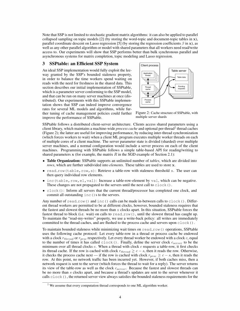
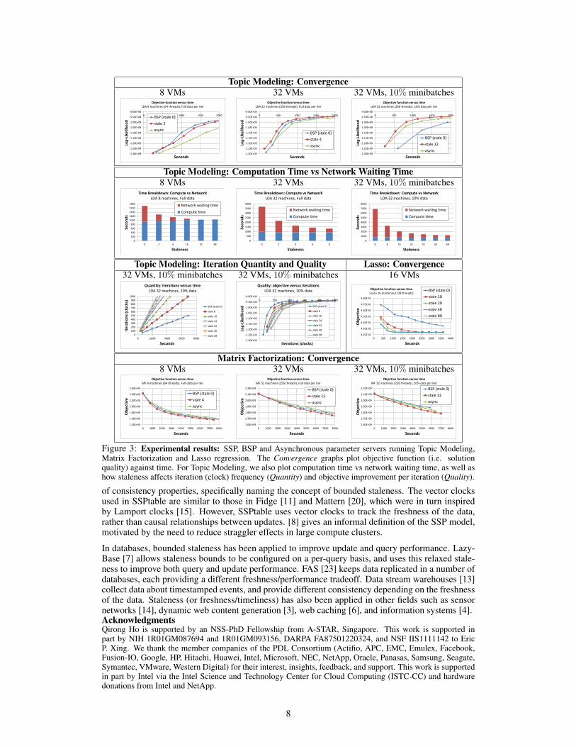
Convergence Speed. Figure 3 shows objective vs. time plots for the three ML algorithms, overseveral machine configurations. We are interested in how long each algorithm takes to reach a givenobjective value, which corresponds to drawing horizontal lines on the plots. On each plot, we showcurves for BSP (zero staleness), Async, and SSP for the best staleness value ≥ 1 (we generallyomit the other SSP curves to reduce clutter). In all cases except Topic Modeling with 8 VMs, SSPconverges to a given objective value faster than BSP or Async. The gap between SSP and the othersystems increases with more VMs and smaller data batches, because both of these factors lead toincreased network communication — which SSP is able to reduce via staleness. We also provide ascalability-with-N -machines plot in the Appendix.Computation Time vs Network Waiting Time. To understand why SSP performs better, we lookat how the Topic Modeling (TM) algorithm spends its time during a fixed number of clock()s. Inthe 2nd row of Figure 3, we see that for any machine configuration, the TM algorithm spends roughlythe same amount of time on useful computation, regardless of the staleness value. However, the timespent waiting for network communication drops rapidly with even a small increase in staleness,allowing SSP to execute clock()s more quickly than BSP (staleness 0). Furthermore, the ratio ofnetwork-to-compute time increases as we add more VMs, or use smaller data batches. At 32 VMsand 10% data minibatches, the TM algorithm under BSP spends six times more time on networkcommunications than computation. In contrast, the optimal value of staleness, 32, exhibits a 1:1ratio of communication to computation. Hence, the value of SSP lies in allowing ML algorithmsto perform far more useful computations per second, compared to the BSP model (e.g. Hadoop).Similar observations hold for the MF and Lasso applications (graphs not shown for space reasons).Iteration Quantity and Quality. The network-compute ratio only partially explains SSP’s behav-ior; we need to examine each clock()’s behavior to get a full picture. In the 3rd row of Figure 3,we plot the number of clocks executed per worker per unit time for the TM algorithm, as well asthe objective value at each clock. Higher staleness values increase the number of clocks executedper unit time, but decrease each clock’s progress towards convergence (as suggested by our theory);MF and Lasso also exhibit similar behavior (graphs not shown). Thus, staleness is a tradeoff be-tween iteration quantity and quality — and because the iteration rate exhibits diminishing returnswith higher staleness values, there comes a point where additional staleness starts to hurt the rate ofconvergence per time. This explains why the best staleness value in a given setting is some constant0 < s < ∞— hence, SSP can hit a “sweet spot” between quality/quantity that BSP and Async donot achieve. Automatically finding this sweet spot for a given problem is a subject for future work.6 Related Work and DiscussionThe idea of staleness has been explored before: in ML academia, it has been analyzed in the con-text of cyclic-delay architectures [17, 1], in which machines communicate with a central server (oreach other) under a fixed schedule (and hence fixed staleness). Even the bulk synchronous paral-lel (BSP) model inherently produces stale communications, the effects of which have been studiedfor algorithms such as Lasso regression [5] and topic modeling [2]. Our work differs in that SSPadvocates bounded (rather than fixed) staleness to allow higher computational throughput via localmachine caches. Furthermore, SSP’s performance does not degrade when parameter updates fre-quently collide on the same vector elements, unlike asynchronous lock-free systems [21]. We notethat staleness has been informally explored in the industrial setting at large scales; our work providesa first attempt at rigorously justifying staleness as a sound ML technique.

Distributed platforms such as Hadoop and GraphLab [18] are popular for large-scale ML. Thebiggest difference between them and SSPtable is the programming model — Hadoop uses a statelessmap-reduce model, while GraphLab uses stateful vertex programs organized into a graph. In con-trast, SSPtable provides a convenient shared-memory programming model based on a table/matrixAPI, making it easy to convert single-machine parallel ML algorithms into distributed versions. Inparticular, the algorithms used in our experiments — LDA, MF, Lasso — are all straightforwardconversions of single-machine algorithms. Hadoop’s BSP execution model is a special case of SSP,making SSPtable more general in that regard; however, Hadoop also provides fault-tolerance anddistributed filesystem features that SSPtable does not cover. Finally, there exist special-purposetools such as Vowpal Wabbit [16] and YahooLDA [2]. Whereas these systems have been targeted ata subset of ML algorithms, SSPtable can be used by any ML algorithm that tolerates stale updates.

The distributed systems community has typically examined staleness in the context of consistencymodels. The TACT model [26] describes consistency along three dimensions: numerical error, ordererror, and staleness. Other work [24] attempts to classify existing systems according to a number

7

Topic Modeling: Convergence8 VMs 32 VMs 32 VMs, 10% minibatches

-1.30E+09

-1.25E+09

-1.20E+09

-1.15E+09

-1.10E+09

-1.05E+09

-1.00E+09

-9.50E+08

-9.00E+08

0 500 1000 1500 2000

Log-

Like

liho

od

Seconds

Objective function versus time LDA 8 machines (64 threads), Full data per iter

BSP (stale 0)

stale 2

async

-1.30E+09

-1.25E+09

-1.20E+09

-1.15E+09

-1.10E+09

-1.05E+09

-1.00E+09

-9.50E+08

-9.00E+08

0 500 1000 1500 2000

Log-

Like

liho

od

Seconds

Objective function versus time LDA 32 machines (256 threads), Full data per iter

BSP (stale 0)

stale 4

async

-1.30E+09

-1.25E+09

-1.20E+09

-1.15E+09

-1.10E+09

-1.05E+09

-1.00E+09

-9.50E+08

-9.00E+08

0 500 1000 1500 2000

Log-

Like

liho

od

Seconds

Objective function versus time LDA 32 machines (256 threads), 10% data per iter

BSP (stale 0)

stale 32

async

Topic Modeling: Computation Time vs Network Waiting Time8 VMs 32 VMs 32 VMs, 10% minibatches

0

200

400

600

800

1000

1200

1400

1600

1800

0 2 4 16 32 48

Seco

nd

s

Staleness

Time Breakdown: Compute vs Network LDA 8 machines, Full data

Network waiting time

Compute time

0

500

1000

1500

2000

2500

3000

3500

4000

0 2 4 6 8 Se

con

ds

Staleness

Time Breakdown: Compute vs Network LDA 32 machines, Full data

Network waiting time

Compute time

0

1000

2000

3000

4000

5000

6000

7000

8000

0 8 16 24 32 40 48

Seco

nd

s

Staleness

Time Breakdown: Compute vs Network LDA 32 machines, 10% data

Network waiting time

Compute time

Topic Modeling: Iteration Quantity and Quality Lasso: Convergence32 VMs, 10% minibatches 32 VMs, 10% minibatches 16 VMs

0

100

200

300

400

500

600

700

800

900

1000

0 2000 4000 6000 8000

Ite

rati

on

s (c

lock

s)

Seconds

Quantity: iterations versus time LDA 32 machines, 10% data

BSP (stale 0)

stale 8

stale 16

stale 24

stale 32

stale 40

stale 48

-1.30E+09

-1.25E+09

-1.20E+09

-1.15E+09

-1.10E+09

-1.05E+09

-1.00E+09

-9.50E+08

-9.00E+08

0 200 400 600 800 1000

Log-

Like

liho

od

Iterations (clocks)

Quality: objective versus iterations LDA 32 machines, 10% data

BSP (stale 0)

stale 8

stale 16

stale 24

stale 32

stale 40

stale 48 4.20E-01

4.30E-01

4.40E-01

4.50E-01

4.60E-01

4.70E-01

4.80E-01

0 500 1000 1500 2000 2500 3000 3500 4000

Ob

ject

ive

Seconds

Objective function versus time Lasso 16 machines (128 threads)

BSP (stale 0)

stale 10

stale 20

stale 40

stale 80

Matrix Factorization: Convergence8 VMs 32 VMs 32 VMs, 10% minibatches

1.40E+09

1.60E+09

1.80E+09

2.00E+09

2.20E+09

2.40E+09

2.60E+09

0 1000 2000 3000 4000 5000 6000 7000 8000

Ob

ject

ive

Seconds

Objective function versus time MF 8 machines (64 threads), Full data per iter

BSP (stale 0)

stale 4

async

1.60E+09

1.70E+09

1.80E+09

1.90E+09

2.00E+09

2.10E+09

2.20E+09

0 1000 2000 3000 4000 5000 6000 7000 8000

Ob

ject

ive

Seconds

Objective function versus time MF 32 machines (256 threads), Full data per iter

BSP (stale 0)

stale 15

async

1.60E+09

1.70E+09

1.80E+09

1.90E+09

2.00E+09

2.10E+09

2.20E+09

0 1000 2000 3000 4000 5000 6000 7000 8000

Ob

ject

ive

Seconds

Objective function versus time MF 32 machines (256 threads), 10% data per iter

BSP (stale 0)

stale 32

async

Figure 3: Experimental results: SSP, BSP and Asynchronous parameter servers running Topic Modeling,Matrix Factorization and Lasso regression. The Convergence graphs plot objective function (i.e. solutionquality) against time. For Topic Modeling, we also plot computation time vs network waiting time, as well ashow staleness affects iteration (clock) frequency (Quantity) and objective improvement per iteration (Quality).

of consistency properties, specifically naming the concept of bounded staleness. The vector clocksused in SSPtable are similar to those in Fidge [11] and Mattern [20], which were in turn inspiredby Lamport clocks [15]. However, SSPtable uses vector clocks to track the freshness of the data,rather than causal relationships between updates. [8] gives an informal definition of the SSP model,motivated by the need to reduce straggler effects in large compute clusters.

In databases, bounded staleness has been applied to improve update and query performance. Lazy-Base [7] allows staleness bounds to be configured on a per-query basis, and uses this relaxed stale-ness to improve both query and update performance. FAS [23] keeps data replicated in a number ofdatabases, each providing a different freshness/performance tradeoff. Data stream warehouses [13]collect data about timestamped events, and provide different consistency depending on the freshnessof the data. Staleness (or freshness/timeliness) has also been applied in other fields such as sensornetworks [14], dynamic web content generation [3], web caching [6], and information systems [4].AcknowledgmentsQirong Ho is supported by an NSS-PhD Fellowship from A-STAR, Singapore. This work is supported inpart by NIH 1R01GM087694 and 1R01GM093156, DARPA FA87501220324, and NSF IIS1111142 to EricP. Xing. We thank the member companies of the PDL Consortium (Actifio, APC, EMC, Emulex, Facebook,Fusion-IO, Google, HP, Hitachi, Huawei, Intel, Microsoft, NEC, NetApp, Oracle, Panasas, Samsung, Seagate,Symantec, VMware, Western Digital) for their interest, insights, feedback, and support. This work is supportedin part by Intel via the Intel Science and Technology Center for Cloud Computing (ISTC-CC) and hardwaredonations from Intel and NetApp.

8

References[1] A. Agarwal and J. C. Duchi. Distributed delayed stochastic optimization. In Decision and Control (CDC),

2012 IEEE 51st Annual Conference on, pages 5451–5452. IEEE, 2012.[2] A. Ahmed, M. Aly, J. Gonzalez, S. Narayanamurthy, and A. J. Smola. Scalable inference in latent variable

models. In WSDM, pages 123–132, 2012.[3] N. R. Alexandros Labrinidis. Balancing performance and data freshness in web database servers. pages

pp. 393 – 404, September 2003.[4] M. Bouzeghoub. A framework for analysis of data freshness. In Proceedings of the 2004 international

workshop on Information quality in information systems, IQIS ’04, pages 59–67, 2004.[5] J. K. Bradley, A. Kyrola, D. Bickson, and C. Guestrin. Parallel coordinate descent for l1-regularized loss

minimization. In International Conference on Machine Learning (ICML 2011), June 2011.[6] L. Bright and L. Raschid. Using latency-recency profiles for data delivery on the web. In Proceedings of

the 28th international conference on Very Large Data Bases, VLDB ’02, pages 550–561, 2002.[7] J. Cipar, G. Ganger, K. Keeton, C. B. Morrey, III, C. A. Soules, and A. Veitch. LazyBase: trading

freshness for performance in a scalable database. In Proceedings of the 7th ACM european conference onComputer Systems, pages 169–182, 2012.

[8] J. Cipar, Q. Ho, J. K. Kim, S. Lee, G. R. Ganger, G. Gibson, K. Keeton, and E. Xing. Solving the stragglerproblem with bounded staleness. In HotOS ’13. Usenix, 2013.

[9] J. Dean, G. Corrado, R. Monga, K. Chen, M. Devin, Q. Le, M. Mao, M. Ranzato, A. Senior, P. Tucker,K. Yang, and A. Ng. Large scale distributed deep networks. In NIPS 2012, 2012.

[10] Facebook. www.facebook.com/note.php?note_id=10150388519243859, January 2013.[11] C. J. Fidge. Timestamps in Message-Passing Systems that Preserve the Partial Ordering. In 11th Aus-

tralian Computer Science Conference, pages 55–66, University of Queensland, Australia, 1988.[12] R. Gemulla, E. Nijkamp, P. J. Haas, and Y. Sismanis. Large-scale matrix factorization with distributed

stochastic gradient descent. In KDD, pages 69–77. ACM, 2011.[13] L. Golab and T. Johnson. Consistency in a stream warehouse. In CIDR 2011, pages 114–122.[14] C.-T. Huang. Loft: Low-overhead freshness transmission in sensor networks. In SUTC 2008, pages

241–248, Washington, DC, USA, 2008. IEEE Computer Society.[15] L. Lamport. Time, clocks, and the ordering of events in a distributed system. Commun. ACM, 21(7):558–

565, July 1978.[16] J. Langford, L. Li, and A. Strehl. Vowpal wabbit online learning project, 2007.[17] J. Langford, A. J. Smola, and M. Zinkevich. Slow learners are fast. In Advances in Neural Information

Processing Systems, pages 2331–2339, 2009.[18] Y. Low, G. Joseph, K. Aapo, D. Bickson, C. Guestrin, and M. Hellerstein, Joseph. Distributed GraphLab:

A framework for machine learning and data mining in the cloud. PVLDB, 2012.[19] G. Malewicz, M. H. Austern, A. J. Bik, J. C. Dehnert, I. Horn, N. Leiser, and G. Czajkowski. Pregel: a

system for large-scale graph processing. In Proceedings of the 2010 International Conference on Man-agement of Data, pages 135–146. ACM, 2010.

[20] F. Mattern. Virtual time and global states of distributed systems. In C. M. et al., editor, Proc. Workshopon Parallel and Distributed Algorithms, pages 215–226, North-Holland / Elsevier, 1989.

[21] F. Niu, B. Recht, C. Re, and S. J. Wright. Hogwild!: A lock-free approach to parallelizing stochasticgradient descent. In NIPS, 2011.

[22] R. Power and J. Li. Piccolo: building fast, distributed programs with partitioned tables. In Proceedingsof the USENIX conference on Operating systems design and implementation (OSDI), pages 1–14, 2010.

[23] U. Rohm, K. Bohm, H.-J. Schek, and H. Schuldt. Fas: a freshness-sensitive coordination middleware fora cluster of olap components. In VLDB 2002, pages 754–765. VLDB Endowment, 2002.

[24] D. Terry. Replicated data consistency explained through baseball. Technical Report MSR-TR-2011-137,Microsoft Research, October 2011.

[25] Yahoo! http://webscope.sandbox.yahoo.com/catalog.php?datatype=g, 2013.[26] H. Yu and A. Vahdat. Design and evaluation of a conit-based continuous consistency model for replicated

services. ACM Transactions on Computer Systems, 20(3):239–282, Aug. 2002.[27] M. Zaharia, M. Chowdhury, M. J. Franklin, S. Shenker, and I. Stoica. Spark: cluster computing with

working sets. In Proceedings of the 2nd USENIX conference on Hot topics in cloud computing, 2010.[28] M. Zinkevich, M. Weimer, A. Smola, and L. Li. Parallelized stochastic gradient descent. Advances in

Neural Information Processing Systems, 23(23):1–9, 2010.

9