MORE CONFIDENCE IN SALARIES IN PETROLEUM ENGINEERING · MORE CONFIDENCE IN SALARIES IN PETROLEUM ENGINEERING ... Petroleum Engineering”, then you can skip Part 1 and only complete

_____________________________________________________________________________________________

STatistics Education Web: Online Journal of K-12 Statistics Lesson Plans 1

http://www.amstat.org/education/stew/

Contact Author for permission to use materials from this STEW lesson in a publication

MORE CONFIDENCE IN

SALARIES IN PETROLEUM

ENGINEERING Susan A. Peters AnnaMarie Conner

University of Louisville University of Georgia

[email protected] [email protected]

Published: October, 2016

Overview of Lesson

This lesson follows from the “Confidence in Salaries in Petroleum Engineering” lesson, and

introduces students to randomization tests for making inferences about a population parameter

using a randomly selected sample from the population. Students use random samples of salaries

for petroleum engineering graduates and technology tools to conduct a significance test to

determine whether petroleum engineering graduates after 2014 suffered lower starting salaries in

alignment with falling crude oil prices than the 2014 population mean starting salary of

petroleum engineering graduates. They also explore connections between significance tests and

confidence intervals. Students draw conclusions using both the context of the activities and one-

sided and two-sided randomization tests using simulations.

GAISE Components

This investigation follows the four components of statistical problem solving put forth in the

Guidelines for Assessment and Instruction in Statistics Education (GAISE) Report. The four

components are: formulate a question, design and implement a plan to collect data, analyze the

data, and interpret results in the context of the original question.

This is a GAISE Level C activity.

Common Core State Standards for Mathematical Practice

2. Reason abstractly and quantitatively.

3. Construct viable arguments and critique the reasoning of others.

4. Model with mathematics.

5. Use appropriate tools strategically.

Learning Objectives Alignment with Common Core and NCTM PSSM

Learning Objectives Common Core State

Standards

NCTM Principles and

Standards for School

Mathematics

Students will construct a distribution

of sample means using a random

sample.

S-IC.B.5. Use data from a

randomized experiment to

compare two treatments;

Develop and evaluate

inferences and

predictions that are based


mailto:[email protected]

mailto:[email protected]

_____________________________________________________________________________________________




use simulations to decide

if differences between

parameters are significant.

on data:

Use simulations to

explore the variability

of sample statistics

from a known

population and to

construct sampling

distributions.

Students will use a randomization test

to draw conclusions about a

hypothesized population mean or

proportion.

S-IC.B.5. Use data from a

randomized experiment to

compare two treatments;

use simulations to decide

if differences between

parameters are significant.

Develop and evaluate

inferences and

predictions that are based

on data:

Understand how sample

statistics reflect the

values of population

parameters and use

sampling distributions

as the basis for informal

inference.

Students will describe the relationship

between conclusions drawn about a

population mean or proportion for a

95% confidence interval and a

significance test at the 5% level.

Prerequisites

Students should know how to calculate and interpret numerical summary values for one variable

data (mean, standard deviation, median, interquartile range) and know how to construct and

interpret graphical displays of data including dotplots. Students should have some familiarity

with data collection methods such as surveying and important constructs and concepts related to

data collection including random sampling and representative samples. Students who have

previously conducted simulations and encountered sampling distributions will benefit most from

this lesson. Prior to this lesson, students should have completed the “Confidence in Salaries in

Petroleum Engineering” lesson or have experience with using bootstrapping methods and

technology tools to calculate and interpret interval estimates for a population mean and

population proportion. If students have completed the lesson “Confidence in Salaries in

Petroleum Engineering”, then you can skip Part 1 and only complete Part 2 of this lesson. If not,

students will benefit from engaging in informal inference with the sample data in Part 1.


_____________________________________________________________________________________________




Time Required

This two-part lesson will require about 100-150 minutes per part, with Part 1 requiring two 50-

minute class periods and Part 2 requiring two to three 50-minute class periods. One additional

class period would be needed for the suggested assessment.

NOTE: If students completed the “Confidence in Salaries in Petroleum Engineering” lesson, then

you can skip Part 1. You may also choose to skip the physical simulation done with cards if they

did this similar activity in the “Confidence in Salaries in Petroleum Engineering” lesson.

Materials and Preparation Required

Pencil and paper

One deck of cards per student group

Randomization software or Internet access (directions in this lesson will refer to a

StatKey applet http://lock5stat.com/statkey)

Calculator or statistics software for computing statistics and graphing data

Post-it notes to record class data

Large number lines to display dotplots of class data


http://lock5stat.com/statkey

_____________________________________________________________________________________________




More Confidence in Salaries in Petroleum Engineering

Teacher’s Lesson Plan

Part 1: Informal Inference

(Note: If students have completed the lesson “Confidence in Salaries in Petroleum Engineering”,

then you can skip Part 1 in this lesson and only complete Part 2. If not, students will benefit from

engaging in informal inference with the sample data in Part 1.)

Describe the Context and Formulate a Question

Ask students to consider different professions they might consider for their futures and why.

Students might mention different professions based on salary and job availability. Inform

students that a job in petroleum engineering might be appealing to them. According to a survey

conducted by the National Association of Colleges and Employers (NACE, 2015b), bachelor

degree graduates from the class of 2014 who earned the highest average (mean) starting salary of

$86,266 were those who majored in petroleum engineering. Ask students what other information

they might want to know about the petroleum engineering profession. Focus on information that

might help students to determine whether the profession might be a good choice for them.

Ask students to state specific questions about the petroleum engineering profession that could be

answered with data. Focus students on salaries and job availability as two important

characteristics for considering the viability of the major and graduates’ likelihood of achieving

this mean salary. Ask students whether they believe the $86,266 mean starting salary would be

the current mean starting salary or whether the salary might have increased or decreased based

on current market demands. Ask students to consider various factors that could affect starting

salaries of petroleum engineering graduates. The NACE (2015b) survey also suggested that 43

out of the 277 petroleum-engineering graduates in 2014 were still seeking employment at the

time of the survey. Ask students whether they believe that this figure from 2014 is still valid

today. Students may be aware that towards the end of 2015, crude oil prices dropped

(http://www.cnbc.com/2015/12/04/petroleum-engineering-degrees-seen-going-from-boom-to-

bust.html), raising the question of whether the drop in oil prices also precipitated a drop in

salaries or job availability at energy firms that employ petroleum engineers.

The activities that follow are based on answering the following questions: Is the current average

starting salary for graduates majoring in petroleum engineering less than $86,266? Does the

current average starting salary for graduates majoring in petroleum engineering differ from

$86,266? Is the current proportion of petroleum-engineering graduates who are employed less

than 84.5%?


http://www.cnbc.com/2015/12/04/petroleum-engineering-degrees-seen-going-from-boom-to-bust.html


_____________________________________________________________________________________________




Collect Data

This lesson does not involve direct data collection for the sample of 16 randomly selected

starting salaries of petroleum engineering graduates that students will use in lesson activities.

However, students will consider data collection techniques that allow inferences for a population

to be made from a sample.

Distribute the “Analyzing Data from a Single Sample” activity sheet, and ask students to work in

pairs or in groups to answer the items on the activity sheet. Make sure that students have a

calculator or software to calculate summary values. After students have a chance to answer the

questions, discuss their responses. You may wish to begin discussions with item (1), which is

discussed below in the “Analyze Data” and “Interpret Results” sections, or with item (3).

Item (3) from the activity is intended to directly address the issue of data collection. Poll students

about what methods they believe would yield representative samples. An important aspect of any

data collection method that should be mentioned is random selection. Although students might

suggest different methods to increase representativeness such as stratifying graduates according

to the type of institution from which they graduated, there still may be lurking variables that

interfere with selecting a representative sample. Random selection is designed to control the

effects of unidentified factors by ensuring equal probabilities for selecting units exhibiting these

factors (or not) and provides the best means for achieving samples representative of their

respective populations. This particular item is intended to focus students on the difference

between a sample and a population and the importance of using random and representative

samples to make inferences about a population. If students suggest that we should have worked

with the population of all post-2014 petroleum engineering graduates, ask students to generate

reasons why collecting data from the population of all graduates, particularly data about salaries,

may not be feasible or possible.

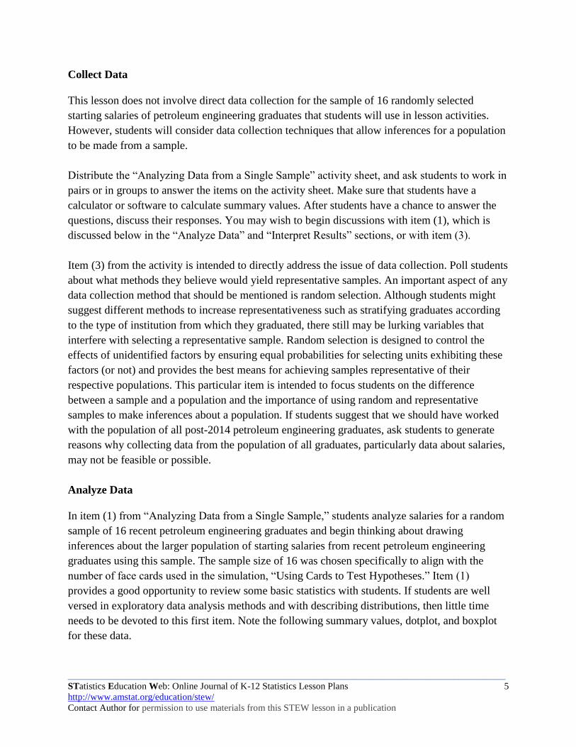
Analyze Data

In item (1) from “Analyzing Data from a Single Sample,” students analyze salaries for a random

sample of 16 recent petroleum engineering graduates and begin thinking about drawing

inferences about the larger population of starting salaries from recent petroleum engineering

graduates using this sample. The sample size of 16 was chosen specifically to align with the

number of face cards used in the simulation, “Using Cards to Test Hypotheses.” Item (1)

provides a good opportunity to review some basic statistics with students. If students are well

versed in exploratory data analysis methods and with describing distributions, then little time

needs to be devoted to this first item. Note the following summary values, dotplot, and boxplot

for these data.


_____________________________________________________________________________________________




N Mean SE Mean StDev Minimum Q1 Median Q3 Maximum

16 80603.06 5773.45 23093.80 35000.00 65087.00 93750.00 100000.00 106475.00

*Note that these sample characteristics are consistent with starting salary projections for

petroleum engineering graduates in the class of 2015 (NACE, 2015c).

Interpret Results

These data are somewhat skewed left, so the median and interquartile range might be best for

describing these data. However, the lack of outliers suggests that the mean and standard

deviation are not entirely inappropriate for describing the distribution. Use a Whip Around

strategy to have groups share their descriptions from (1) by randomly selecting groups to share

one observation about the distribution and continuing in this manner until all ideas have been

shared. As students present their responses, press them to not only report statistics but also to

interpret the meaning of the measures. For example, the mean of approximately $80,603 means

that if every one of the 16 engineers earned the same salary, they would each earn a salary of

$80,603. This is not the case, however, as the approximate average deviation from the mean is

$23,093.80. The middle 50% of salaries fall in the interval between $65,087 and $100,000. The

person earning the least in this sample earns $35,000, which is $71,475 less than the person

earning the maximum of $106,475.

As students continue to share their responses to items (2) through (4), focus students on the idea

that sample characteristics rarely, if ever, are equivalent to the population characteristics,

whether the population is salaries from the NACE survey, salaries from some other population,

or units different from salaries. Therefore, a sample mean is not likely to equal a population

mean; however, without additional information about a population, a sample mean provides a

reasonable estimate for the population mean. Introduce the idea of sampling variability—that

samples and their characteristics such as shape, measures of center, and measure of variation are

likely to vary from sample to sample in repeated sampling—to suggest that this sample of size 16

could have been selected from the population of starting salaries of petroleum engineering

graduates with mean $86,266. If students consider the variability between the sample mean and

population mean to be too great for the sample of size 16 to have been selected from the same

population, ask students to speculate about what sample means would suggest samples selected


_____________________________________________________________________________________________




from the population of salaries with mean $86,266. Point out that inference techniques present

criteria for making these types of decisions.

Items (5) and (6) set up the idea of using samples to make inferences about populations. Point

out to students that we typically don’t expect sample means to equal population means. The real

question is whether a sample mean provides evidence to doubt a posited value for a population

mean. Inform students that they will explore one method—using a test of significance—to test

whether an observed characteristic of sample data could have occurred by chance or is indicative

of a population parameter different from what was assumed. In particular, they will conduct a

randomization test. Remind students that we will perform these analyses under the assumption

that our sample data are representative of the larger population from which they were drawn.

Part 2: Randomization Test

Describe the Context and Formulate a Question

Before introducing the randomization test to students, revisit the questions that are the focus of

this series of activities: Is the current average starting salary for graduates majoring in petroleum

engineering less than $86,266? Does the current average starting salary for graduates majoring in

petroleum engineering differ from $86,266? Is the current proportion of petroleum-engineering

graduates who are employed less than 84.5%? To begin, focus students on the first question.

Distribute the “Hypothesizing about Salaries” handout to students, and ask students to read the

information contained in the box. Inform students that they will be conducting a test of

significance, but in order to do so, they must first make their hypotheses about what they are

testing clear. These hypotheses follow directly from the question under investigation. Ask

students to complete items (1) through (4). After students complete these items, ask them for

their null hypotheses, and record all of the different hypotheses offered by students. You may

have students vote on the possibilities to determine the number of students who agree with each

listed hypothesis. Before revealing the correct null hypothesis, ask students which population

value is of interest when addressing the question of whether the current average starting salary

for graduates majoring in petroleum engineering is less than $86,266. In particular, make sure

that students know that the value of $86,266 is the hypothesized value of the population mean,

notated as . Poll students again to lead them to the null hypothesis of H0: = 86,266.

Next, ask students for their alternative hypotheses, and record all of the different hypotheses

offered by students. You may again wish to have students vote on the possibilities to determine

the number of students who agree with each listed hypothesis. Before revealing the correct

alternative hypothesis, ask students to consider which alternative to = 86,266 is of interest

when addressing the question of whether the current average starting salary for graduates


_____________________________________________________________________________________________




majoring in petroleum engineering is less than $86,266. Poll students again to lead them to the

alternative hypothesis of H1: < 86,266.

After recording correct null and alternative hypotheses, poll students about probabilities that they

associate with rare events. Remind students that a significance test yields an estimate of the

probability that an observed data characteristic occurred by chance—that an observed data

characteristic is rare under the assumed condition of the null hypothesis. Then ask students to

read the information in the box that appears after item (4) and to complete items (5) and (6). This

appears here as well:

A low probability that a sample statistic occurred by chance raises questions about

the truth or validity of the null hypothesis. Many statisticians begin to question

chance occurrence with probabilities that are less than 0.05 or 0.01, which are

typical threshold values that statisticians use when considering the null

hypothesis. This threshold probability value is called the alpha level or the

significance level and is typically noted as . When we observe probabilities less

than , we typically reject the null hypothesis in favor of the alternative

hypothesis. Alternatively, when we observe probabilities greater than or equal to

, we have not proven that our null hypothesis is true but fail to reject the null

hypothesis because we do not have sufficient evidence to accept the alternative.

After students complete these two items, ask how many students believe that they should reject a

null hypothesis given a probability (also known as a p-value) of 0.025 and how many students

believe that they should fail to reject the null hypothesis. Ask the questions again, specifying an

level of 0.05. Repeat for an level of 0.01. Note that with a p-value of 0.025, students should

reject the null hypothesis for an level of 0.05 and fail to reject the null hypothesis for an

level of 0.01. Remind students that if they reject the null hypothesis, they accept the alternative

hypothesis that the population mean starting salary of recent petroleum engineering graduates is

less than $86,266. If they fail to reject the null hypothesis, they do not have sufficient evidence to

accept the alternative hypothesis. That is, they do not have sufficient evidence to suggest that the

population mean starting salary of recent petroleum engineering graduates is less than $86,266.

Item (6) is intended to have students think about possible ways to determine probabilities.

Depending upon their previous experiences, students might suggest obtaining a larger sample or

additional samples to better estimate the probability.

Collect Data

Students will use sampling with replacement to select samples towards determining whether the

average starting salary of all recent graduates majoring in petroleum engineering could be


_____________________________________________________________________________________________




$86,266. Point out to students that the only data they have available to them is the data from this

single sample. Revisit the idea of representativeness to have students consider what the

population distribution might be if the sample truly were representative of the population. (Note

that they would likely estimate the population mean to be close in value to the sample mean,

which would not be close in value to the hypothesized population mean of $86,266. Do not yet

point this out to students.) Lead in to the idea of randomization by asking students to consider

how they might use this single sample to obtain additional samples. Ask students to read the

information contained in the box before item (7) and then to complete item (7).

Engage students in a think-pair-share to think about, discuss, and share methods for sampling

with replacement. Students may suggest strategies such as creating slips of paper for each salary

and selecting slips (with replacement) from a hat. If students previously worked with random

number tables, they may suggest assigning numbers to each possible outcome and using a

random number table to simulate sampling with replacement. For each strategy presented, ask

students to be explicit in describing how each of the 16 salaries is represented, how the process

incorporates randomization (so that each of the 16 salaries has the same probability of being

selected), and how the process incorporates the idea of replacement so that each of the 16 values

can be selected for each of the 16 selections.

Note: From this point forward, we refer to the original 16 salaries as a sample of salaries. Our

use of this terminology is an abbreviated way of saying that the salaries were reported by a

sample of recent petroleum engineering graduates from the population of all recent petroleum

engineering graduates. The sampling unit is the graduate, but the observational unit is the salary.

Students may pick up on this slight change in wording.

Note that the randomization process and using sample data as if it were population data may not

be intuitive for students. Remind students that ideally we would work with the population

directly; because we realistically can only work from the sample, we try to approximate

characteristics of the population as closely as possible by using sample data. In this way, students

can consider the population to be many copies of the sample. Rather than make copies of the

sample, we use sampling with replacement to repeatedly resample from our sample. In the case

of salaries for recent petroleum engineering graduates, we will need to assume that each starting

salary from the sample represents many similar starting salaries from the population of all recent

petroleum engineering graduates’ salaries. Because we want to examine a distribution of means

centered at the hypothesized value of $86,266 to see where our sample mean falls in this

distribution and because we are using our sample as a best estimate for a population, however,

we need a sample that has this hypothesized population mean of $86,266. Because our sample

mean is $5,663 lower than the hypothesized mean, we add $5,663 to each data value in our

sample to simulate a distribution centered at $86,266—a set of data consistent with the null

hypothesis— and sample with replacement from this distribution.


_____________________________________________________________________________________________




Distribute the “Using Cards to Test Hypotheses” activity sheet to students. Ask students to read

the information displayed in the box at the top of the first page. After students complete reading,

ask different students to paraphrase key sentences (e.g., the first sentence and what it means to

conduct a significance test in this context) until students seem to understand what they are testing

and how they are using the original sample data in their simulations.

(** Note: Students who completed the series of activities for “Confidence in Salaries in

Petroleum Engineering” may not need to conduct the physical simulation. Although they may be

able to skip the simulation work for “Using Cards to Test Hypotheses,” they should read and

discuss the information presented in the box on the first page of the activity sheet. **)

Ask students to complete the activity sheet. Students will use a deck of cards to simulate

sampling with replacement from the sample of 16 adjusted salaries [items (1) through (7) for

“Using Cards to Test Hypotheses”]. Research suggests that performing simulations by hand

before using technology can aid students in understanding the conceptual ideas that underlie

statistical inference (Pfannkuch, Forbes, Harraway, Budgett, & Wild, 2013). Students will

combine their results with those from the rest of the class to estimate the probability of observing

a mean as low or lower than the sample mean from the original sample of salaries [items (8)

through (12) for “Using Cards to Test Hypotheses”]. Prior to beginning this activity, display a

large number line such as the number line displayed in item (8) in the classroom. As students are

working, circulate around the room, and when you notice that students have recorded their four

means in item (5), ask them to record their sample means on post-it notes and position the post-it

notes as dots above the large number line to create a dotplot of simulation results from the class.

As part of the simulation process, students compare one or more simulated randomization sample

salaries with the adjusted sample salaries to reinforce the notion of sampling variability [item

(2)]. While they are working, encourage students to consider the shape, center, and variation of

the randomization samples in comparison with the adjusted sample. Students should observe

differences in these characteristics, but ask them to focus on the variability in the samples in

comparison with the variability in characteristics. Students create dotplots from the

randomization sample means to begin creating a randomization distribution; asking students to

compare the variability of the samples with the variability of the randomization distribution can

help students to see the reduced variation in a distribution of means.

After students complete the activity, focus discussion on items (11) and (12). If students do not

express greater confidence for suggesting a probability estimate from the class display, question

students about how the size of a sample affects their confidence for describing distribution

characteristics. Just as larger samples instill greater confidence for drawing inferences about

populations, larger distributions of statistics instill greater confidence for drawing inferences


_____________________________________________________________________________________________




about parameters. The randomization distribution of sample means from (8) is a distribution of a

sample of sample means. Students should have greater confidence in estimating a probability

from the dotplot displaying sample means from the class, which should then motivate additional

simulation.

Analyze Data

Students will need Internet access and computing technology in the form of a laptop or tablet to

access the StatKey applets to create a randomization distribution for 1000 sample means.

Students should work with a partner on items (1) through (7) from “Randomizing for

Significance” to conduct a significance test for the population mean starting salary of recent

petroleum engineering graduates.

Interpret Results

After all students have recorded answers to items (1) through (7), ask students to share whether

the value of $80,603 was one of the means in the left tail of their randomization distribution or

would fall within the interval of values in the left tail of their randomization distribution. Then

ask students to respond to the following questions.

1. For how many of the class simulations did the original sample mean of $80,603 fall in the

interval of values for the left tail of the randomization distribution?

2. What does the value of $80,603 falling in the left tail tell us about the probability of

obtaining a mean starting salary equal to the original sample mean or less?

3. What conclusion should we draw based on this probability?

4. What does the value of $80,603 not falling in the left tail tell us about the probability of

obtaining a mean starting salary equal to the original sample mean or less?


With respect to conclusions, emphasize that these conclusions are based on our initial

assumption that the population mean was $86,266. For most, if not all, students, the original

sample mean will not be in the interval of values in the left tail. As a result, most students should

conclude that the probability of drawing a sample with mean of $80,603 or less from a

population of starting salaries for petroleum engineering graduates with a mean of $86,266 is

greater than 5%. They would fail to reject the null hypothesis and conclude that they do not have

sufficient evidence to suggest that the mean starting salary has decreased from 2014. Ask

students how their conclusions might differ if the population mean were larger than $86,266 or if

the population mean were smaller than $86,266 and what value of the population mean might

produce significant results. Point out to students that variation in data also affects abilities to

reject the null hypothesis.


_____________________________________________________________________________________________




Ask students to complete questions 8 through 10 on the Randomizing for Significance activity

sheet. After students have answered the remaining questions, again poll students.

1. For your randomization distribution, what was the probability of selecting a sample with

a mean equal to or less than the original sample mean of $80,603?


Note that students should obtain the same results in terms of significance for item (8) as they did

for item (6). To this point, students have conducted a one-sided test of significance, meaning

they were interested in determining whether the population parameter was greater than or less

than the hypothesized value in the null hypothesis. Item (10) leads into having students consider

a two-sided test. We use a two-sided test when we wish to test whether data support a different

parameter value than specified in the null hypothesis but are not concerned about the direction of

the relationship. At a significance level of 0.05, then we would consider the cutoff values for

significance to be the lower 2.5% and the upper 2.5% of the randomization distribution.

Students who completed the series of activities for “Confidence in Salaries in Petroleum

Engineering” may recall that significance tests are not the only methods used to draw inferences

about population characteristics using samples randomly drawn from the population: confidence

intervals also are used to draw inferences. Ask students whether they believe there is a

relationship between confidence intervals and significance tests. If students believe that a

relationship exists, ask them what they think the relationship might be. Inform them that they

will explore whether a relationship exists in the next activity.

Part 3: Connecting Confidence with Significance

The resampling process used to conduct a significance test is the same as the resampling process

used to construct confidence intervals; the only difference is the shift in sample values used for

resampling with the significance test. We will use the bootstrapping method used in the

“Confidence in Salaries in Petroleum Engineering” lesson to find a 95% confidence interval for

the population mean starting salary for petroleum engineering graduates.

Distribute the “Connecting Confidence with Significance” activity sheet to students. Have

students work in pairs to complete items (1) through (5). As students work, circulate to make

sure that they are selecting the correct options in StatKey for item (1). In particular, focus on

making sure that students enter the data for salaries from the original sample and that they select

the “Right Tail” option in StatKey. Ask each pair of students to record their interval, whether the

interval captured the value of $86,255, their interpretation of the interval, and their conclusions

in relation to the significance test on whiteboards or chart paper.


_____________________________________________________________________________________________




After students complete questions (1) through (5), ask them to conduct a gallery walk, taking

sticky notes along with them. Ask students to read through the information posted by each pair,

to ask clarifying questions for those pairs by recording questions on sticky notes and affixing

them to the posters, and to look for patterns in results. When students complete the gallery walk,

give them an opportunity to revise their answers if necessary. Then conduct a Whip Around to

have students share their responses. Pay particular attention to students’ interpretations of the

confidence interval. Their interpretations should take the form of: “We can be 95% confident

that the population mean starting salary for recent petroleum engineering graduates is less than

$________”. In most cases, students will capture the value of $86,266 in their intervals,

suggesting that the population mean starting salary might not be less than $86,266. Their results

should largely coincide with their tests of significance: If their confidence interval captures the

hypothesized population mean value of $86,266, their results should not have been significant; if

their confidence interval does not capture the hypothesized population mean value of $86,266,

their results should have been significant. Because students are using different distributions of

sample means for the significance test and the confidence interval, there is a (slight) chance that

their results might not agree.

Ask students to complete the activity sheet. Circulate as students are working, and record any

problems that students are having with answering items (6) through (11). Discuss these issues as

needed with individual pairs or with the class. After students complete the activity sheet, ask

each pair to share their conjecture from item (12). Record each of the conjectures. At this point,

do not discuss the conjectures but rather suggest that students will examine another situation and

revisit their conjectures at the conclusion of that activity.

Suggested Assessment

Ask students to complete items (1) through (11) from “Try This on your Own.” Note that the

sample proportion is consistent with figures from 2015 petroleum engineering graduates

according to the Society of Petroleum Engineers (as cited in DiChristopher & Schoen, 2015).

After students finish the items, discuss their results and revisit their conjectures. Ask students

to update their conjectures as needed. Discuss the merits of each conjecture and whether any

work completed to this point would disprove the conjecture. In general, if a one-sided

significance test yields significant results at the level of , then the one-sided (100 - )%

confidence interval should not captures the hypothesized parameter value. If a one-sided

significance test does not yield significant results at the level of , then the one-sided (100 - )%

confidence interval should capture the hypothesized parameter value. If a two-sided significance

test yields significant results at the level of , then the two-sided (100 - )% confidence interval

should not capture the hypothesized parameter value. If a two-sided significance test does not

yield significant results at the level of , then the two-sided (100 - )% confidence interval

should capture the hypothesized parameter value.


_____________________________________________________________________________________________




Possible Differentiation

The lesson in general is targeted for students at GAISE Level C; however, lesson activities

associated with Part 1 could be implemented with students at Level B. These students may need

some additional guidance for representing and describing sample data when “Analyzing Data

from a Single Sample” such as being told which representations and summary statistics to use.

Students at Level B may need greater differentiation for activities associated with Part 2.

Specifically, they may need to discuss the concepts introduced in item (7) of “Hypothesizing

about Salaries” in conjunction with completing the first step of “Using Cards to Test

Hypotheses.” After using cards to sample with replacement, students may be able to consider

additional processes that could be used to sample with replacement. Similarly, after completing

the sixth step of “Using Cards to Test Hypotheses,” students may observe that different samples

yield different population estimates to suggest why many samples are needed to calculate

probabilities for determining the significance of a population characteristic. Students at Level B

also will need to spend some time comparing the sample distribution with the distribution of

means that emerges in “Using Cards to Test Hypotheses.” Similarly, they should make multiple

comparisons between the sample distribution and the distribution of means in “Randomizing for

Significance.” Rather than immediately generating 1000 samples using the software, students

should generate many samples and examine the emerging distribution of means to compare

characteristics of the sample distribution with characteristics of the distribution of sample means.

Differentiation needed for “Connecting Confidence with Significance” and “Try This on your

Own” similarly should focus more on making the situation as concrete as possible and slowly

generating the distributions of statistics and thus focus more on the beginning steps of the

activities than on the later steps.

References

DiChristopher, T., & Schoen, J. W. (2015, December 4). Petroleum engineering degrees seen

going from boom to bust. Retrieved from http://www.cnbc.com/2015/12/04/petroleum-

engineering-degrees-seen-going-from-boom-to-bust.html

Franklin, C., Kader, G., Mewborn, D., Moreno, J., Peck, R., Perry, M., & Scheaffer, R. (2007).

Guidelines for Assessment and Instruction in Statistics Education (GAISE) Report.

Alexandra, VA: American Statistical Association. Retrieved from

http://www.amstat.org/education/gaise/

National Association of Colleges and Employers. (2015a). Spring 2015 Salary Survey Executive

Summary. Bethlehem, PA: Author.

National Association of Colleges and Employers. (2015b). First Destinations for the College

Class of 2014. Bethlehem, PA: Author. Retrieved from




http://www.amstat.org/education/gaise/

_____________________________________________________________________________________________




https://www.naceweb.org/uploadedFiles/Pages/surveys/first-destination/nace-first-

destination-survey-preliminary-report-022015.pdf

National Association of Colleges and Employers. (2015c). NACE salary survey. Bethlehem, PA:

Author. Retrieved from https://www.tougaloo.edu/sites/default/files/page-files/2015-

january-salary-survey.pdf

National Governors Association Center for Best Practices & Council of Chief State School

Officers. (2010). Common Core State Standards for Mathematics. Washington, DC:

Authors. Retrieved from http://www.corestandards.org/wp-

content/uploads/Math_Standards.pdf

National Council of Teachers of Mathematics (NCTM). (2000). Principles and Standards for

School Mathematics. Reston, VA: Author.

Payscale Human Capital. (2015). Petroleum Engineer Salary (United States). Retrieved from

http://www.payscale.com/research/US/Job=Petroleum_Engineer/Salary

Pfannkuch, M., Forbes, S., Harraway, J., Budgett, S., & Wild, C. (2013). “Bootstrapping”

Students’ Understanding of Statistical Inference. Auckland, NZ: Teaching & Learning

Research Initiative. Retrieved from

http://www.tlri.org.nz/sites/default/files/projects/9295_summary%20report.pdf

Further Reading About the Topic

Lock, R. H., Lock, P. F., Morgan, K. L., Lock, E. F., & Lock, D. F. (2013). Statistics: Unlocking

the Power of Data. Hoboken, NJ: Wiley.

Tintle, N., Chance, B. L., Cobb, G. W., Rossman, A. J., Roy, S., Swanson, T., & VanderStoep, J.

(2016). Introduction to statistical investigations. Hoboken, NJ: Wiley.

Wild, C. (2011, November 22). Bootstrapping and randomization: Seeing all the moving parts

[Webinar]. In CAUSEweb Activity Webinar Series. Retrieved from

https://www.causeweb.org/webinar/activity/2011-11/

Zieffler, A., & Catalysts for Change. (2015). Statistical Thinking: A simulation approach to

uncertainty (3rd

edition). Minneapolis, MN: Catalyst Press. Downloadable from

https://github.com/zief0002/Statistical-Thinking


https://www.naceweb.org/uploadedFiles/Pages/surveys/first-destination/nace-first-destination-survey-preliminary-report-022015.pdf

https://www.naceweb.org/uploadedFiles/Pages/surveys/first-destination/nace-first-destination-survey-preliminary-report-022015.pdf

https://www.tougaloo.edu/sites/default/files/page-files/2015-january-salary-survey.pdf

https://www.tougaloo.edu/sites/default/files/page-files/2015-january-salary-survey.pdf

http://www.corestandards.org/wp-content/uploads/Math_Standards.pdf

http://www.corestandards.org/wp-content/uploads/Math_Standards.pdf

http://www.payscale.com/research/US/Job=Petroleum_Engineer/Salary

http://www.tlri.org.nz/sites/default/files/projects/9295_summary%20report.pdf

https://www.causeweb.org/webinar/activity/2011-11/

https://github.com/zief0002/Statistical-Thinking

_____________________________________________________________________________________________




http://www.resumeok.com/engineering-manufacturing-

resume-samples/petroleum-engineer-resume-template/

http://www.occupational-resumes.com/Petroleum-

Engineer-Resume-Finding-a-qualified-Resume-

Writer-for-a.php

More Confidence in Salaries in Petroleum Engineering

Student Handouts

Analyzing Data from a Single Sample

For the class of 2014, bachelor’s degree graduates earning the

highest average (mean) starting salary of $86,266 were those who

majored in petroleum engineering (National Association of Colleges

and Employers [NACE], 2015a). Petroleum engineers often work for

oil companies and oversee retrieval and production methods for oil

and natural gas (Payscale, 2015).

The demand for petroleum

engineers tends to rise and fall with oil prices. As oil prices

increase, consumer demands for cheaper production increase; as

oil prices decrease, so do demands for innovation. In this series of

activities, you will explore whether the drop in crude oil prices at

the end of 2015 was accompanied by a drop in starting salaries for

recent petroleum engineering graduates.

1. Suppose a sample of 16 petroleum engineering majors who graduated after 2014 reported the

following starting salaries: $35,000, $42,500, $55,125, $64,875, $65,299, $67,750, $71,750

$93,750, $93,750, $94,125, $94,500, $99,875, $100,125, $101,250, $103,500, and $106,475.

Represent and describe these sample data.

2. Is the mean salary from this sample equal to the mean salary from 2014 that was reported by

NACE? Should it be? Why or why not?


_____________________________________________________________________________________________




3. What would need to be true about the way these data were collected for these salaries to be

representative of starting salaries for the larger population of recent petroleum engineering

graduates?

4. If the actual mean starting salary for recent petroleum engineers equals the 2014 NACE

estimate of $86,266, could the salaries from #1 have been reported from a sample of

graduates from the population of all recent petroleum-engineering graduates? Why or why

not?

5. Estimate the mean starting salary for all recent petroleum-engineering graduates. On what are

you basing this estimate?

6. Will this estimate for the mean starting salary of the population be equal to the population

mean? Why or why not?


_____________________________________________________________________________________________




Hypothesizing about Salaries

In reality, to definitively determine whether the mean starting salary for recent petroleum

engineering graduates is $86,266, we would need to survey every recent petroleum-engineering

graduate about their starting salary. Realistically, surveying an entire population typically cannot

be done. In the case of surveying graduates to determine their starting salaries, privacy laws

would prohibit colleges and universities from supplying researchers with graduates’ contact

information. Even if populations can be surveyed, the costs associated with doing so often are

prohibitive. We get our best guesses about characteristics of a population from using a sample

randomly selected from the population.

We are interested in whether the actual mean starting salary for recent petroleum engineering

graduates is $86,266 because we suspect that the mean may have decreased after crude oil prices

dropped drastically. The only data that we have

available at this point are the 16 salaries from recent

petroleum-engineering graduates, which you just

analyzed (“Analyzing Data from a Single Sample”).

Assume that this sample was randomly selected from

salaries from a representative group of recent graduates.

Although the sample mean does not equal $86,266,

does it provide evidence to suggest that the mean

starting salary for recent graduates is less than $86,266?

Or, could this sample mean have occurred by chance?

To answer these questions, we need to conduct a test of

significance. A significance test yields an estimate of

the probability that an observed data characteristic

occurred by chance if the hypothesized value is indeed

correct.

To be sure that we are clear about what we are testing, we begin by stating our hypotheses in

terms of the population characteristics we are testing.

1. What population characteristic or parameter is our focus in this setting?

http://eugenieteasley.com/hypothesis/


_____________________________________________________________________________________________




2. We begin significance tests with a hypothesis—the null hypothesis (H0)—that our observed

results occurred by chance, in this case, that the sample mean does not provide evidence of a

reduced population mean. If the sample mean occurred by chance, what do we hypothesize as

the population mean starting salary for recent petroleum-engineering graduates?

H0:

3. We conduct a significance test to determine whether evidence exists to cast doubt on the null

hypothesis to the point where we reject the null hypothesis. The alternative to our null

hypothesis is called the alternative hypothesis, notated as H1 or Ha, and is the hypothesis

about what we believe to be the case about the population characteristic and the hypothesis

that we accept when we reject the null hypothesis. What do we hypothesize about the

population mean starting salary for recent petroleum-engineering graduates?

H1:

4. As indicated above, a significance test yields an estimate of the probability that an observed

data characteristic occurred by chance if the null hypothesis is true. What probability value(s)

might cause us to question whether an observed characteristic such as a sample mean could

have occurred by chance?

A low probability that a sample statistic occurred by chance raises questions about the truth or

validity of the null hypothesis. Many statisticians begin to question chance occurrence with

probabilities that are less than 0.05 or 0.01, which are typical threshold values that statisticians

use when considering the null hypothesis. This threshold probability value is called the alpha

level or the significance level and is typically noted as . When we

observe probabilities less than , we typically reject the null

hypothesis in favor of the alternative hypothesis. Alternatively,

when we observe probabilities greater than or equal to , we have

not proven that our null hypothesis is true but fail to reject the null

hypothesis because we do not have sufficient evidence to accept

the alternative.

5. If the probability of obtaining a sample mean as low as our sample mean or lower is 0.025,

what should we conclude about our hypotheses?

6. How might you go about determining the probability of obtaining a sample mean as low as

our sample mean or lower?

http://www.clipartpanda.com/categories/alpha-clipart


_____________________________________________________________________________________________




We could select additional samples of engineers and

calculate their mean starting salaries to estimate the

probability of obtaining a sample mean that differs from

$86,266 as much as or more than our sample mean.

Because sampling from the population can be

expensive, however, we instead use our best estimate

for the population—the sample—and use it as if it were

the population. We randomly select samples using the

data from our sample, a process called resampling.

Because there are a finite number of values in our

sample, we use sampling with replacement, meaning

that after being selected, each salary is recorded and

returned to the collection before the next salary is

selected at random. We will use the term, randomization

sample, for each randomly selected sample formed by

resampling from the original sample.

7. Describe a process for sampling with replacement that could be used to randomly select 16

salaries from the 16 salaries given in “Analyzing Data from a Single Sample”: $35,000,

$42,500, $55,125, $64,875, $65,299, $67,750, $71,750 $93,750, $93,750, $94,125, $94,500,

$99,875, $100,125, $101,250, $103,500, and $106,475.

http://www.petroleumengineer.at/petroleum-engineer/profile.html


_____________________________________________________________________________________________




Using Cards to Test Hypotheses

We wish to test whether the value of this sample mean is too much less

than the value of the hypothesized mean, 𝐻0: 𝜇 = 86266, to believe that

the population mean could be $86,266. To estimate a reasonable

probability for the chance of obtaining a mean as low or lower than our

sample mean, we need to select many samples and calculate their sample

means.

Because we want to examine a distribution of means centered at the

hypothesized value of $86,266 to see where our sample mean falls in this

distribution and because we are using our sample as a best estimate for a

population, we need a sample that has this hypothesized population mean

of $86,266. Because our sample mean is $5663 less than the hypothesized

mean, we will add $5,663 to each data value in our sample to simulate a

distribution centered at $86,266—a set of data now consistent with the null hypothesis— and

sample with replacement from this distribution. (In reality, we would want

to select all possible resamples to know all possible means that could

result from samples of the population, but doing so often is impractical.

Instead, we work with a large number of resamples.) We simulate the

process for the sake of efficiency.

We will use 16 cards from a deck of cards to represent specific salaries in

order to simulate sampling with replacement from our sample of 16

salaries. In particular, we will use the aces and face cards of the four card

suits to represent each of the salaries as shown on the “Resampling

Simulation” page. To begin, remove the aces and face cards from your

deck of cards.

1. Record the values of the sample of 16 salaries that is consistent with the null hypothesis and

that we will use for resampling.

http://www.numericana.com/answer/cards.htm

http://beaed.com/Products/Signage/Safet

ySigns/tabid/1097/CategoryID/434/List/

0/Level/a/ProductID/5426/Default.aspx?

SortField=ProductName%2CProductNa

me


_____________________________________________________________________________________________




2. Simulate the selection of a sample of size 16 using resampling.

a. Shuffle the 16 aces and face cards, and randomly select one of the cards.

b. Record a tally mark for this card in the appropriate box for Sample 1 on the next page.

c. Replace the card.

d. Repeat the selection and recording process (a-c) 15 more times until you have a total of

16 tally marks.

e. Calculate the mean for the 16 salaries selected, and record the value in the table.

3. Compare and contrast this randomization sample with the sample of size 16 from which you

resampled. Focus on the distribution of values and on the mean.

4. Repeat the resampling process (#2) three more times, recording your results in the tables on

the next page.

5. Examine the four means that you calculated for your four randomization samples by first

plotting the means on a dotplot.

6. Use these means to estimate the probability of observing a mean as low or lower than our

original sample mean. Record your estimate here. What would you conclude about your

hypotheses based on this estimate?

7. Would your estimate change if you had calculated additional means? Why or why not?


_____________________________________________________________________________________________




Resampling Simulation

Card Hearts Clubs Diamonds Spades

Ace King Queen Jack Ace King Queen Jack Ace King Queen Jack Ace King Queen Jack

Salary $40,663 $48,163 $60,788 $70,538 $70,962 $73,413 $77,413 $99,413 $99413 $99,788 $100,163 $105,538 $105,788 $106,913 $109,163 $112,138

Sample 1



Salary $40,663 $48,163 $60,788 $70,538 $70,962 $73,413 $77,413 $99,413 $99413 $99,788 $100,163 $105,538 $105,788 $106,913 $109,163 $112,138

Tally

Mean

Sample 2



Salary $40,663 $48,163 $60,788 $70,538 $70,962 $73,413 $77,413 $99,413 $99413 $99,788 $100,163 $105,538 $105,788 $106,913 $109,163 $112,138

Tally

Mean

Sample 3



Salary $40,663 $48,163 $60,788 $70,538 $70,962 $73,413 $77,413 $99,413 $99413 $99,788 $100,163 $105,538 $105,788 $106,913 $109,163 $112,138

Tally

Mean

Sample 4



Salary $40,663 $48,163 $60,788 $70,538 $70,962 $73,413 $77,413 $99,413 $99413 $99,788 $100,163 $105,538 $105,788 $106,913 $109,163 $112,138

Tally

Mean


_____________________________________________________________________________________________




8. Record the value of each mean you calculated on a separate post-it note. Use your post-it

notes to plot your four means on the class display. Examine the class distribution of means,

and record it below.

9. Use the class means to estimate the probability of observing a mean as low or lower than our

observed sample mean. Record your estimate here. What would you conclude about your


10. Compare and contrast this probability and your conclusions with your probability and

conclusions from #6.

11. With which estimate are you more confident for drawing conclusions about recent petroleum

engineering graduates’ starting salaries and why?

12. How many means did you record on your dotplot in #8?


_____________________________________________________________________________________________




Randomizing for Significance

To estimate the probability of selecting a sample with a mean as low as or lower than our

original sample mean when the null hypothesis is true, we need hundreds of randomization

sample means—realistically, 1000 or more. Even though the cards can help us to select samples

quickly, the card process would be quite tedious and frustrating to use for finding 1000 sample

means. We need many more means than we reasonably can gather from using simulations with

materials such as cards. Instead, we use computing technology to simulate

the selection of 1000 or more samples and calculate their means to form a

randomization distribution of means. A nice collection of applets for

resampling, StatKey, is freely available at http://lock5stat.com/statkey/

Go to the StatKey website, and under the heading of

“Randomization Hypothesis Tests,” select the option of “Test

for Single Mean.” To draw inferences about a population, we

use our original sample data with $5,663 added to each value,

for the sample to have a mean of $86,266. (As a reminder,

these adjusted salaries are: $40,663, $48,163, $60,788,

$70,538, $70,962, $73,413, $77,413, $99,413, $99,413,

$99,788, $100,163, $105,538, $105,788, $106,913, $109,163,

and $112,138.) We wish to test whether the mean of the

original sample is too much less than the hypothesized mean, 𝐻0: 𝜇 = 86266, to believe that the

value of $86,266 could be the population mean. We want to examine a distribution of means

centered at the hypothesized value of $86,266 and examine where our original sample mean

would fall in this distribution.

We use these data that are consistent with the null hypothesis as if they

were the population data with a mean of $86,266 to generate a probability

estimate for testing the null hypothesis, 𝐻0: 𝜇 = 86266, against the

alternative hypothesis, 𝐻1: 𝜇 < 86266. We then resample from these data,

record the means, and plot the means to form a randomization distribution.

We use StatKey to create this distribution by following the steps listed below.

a. Click on the “Edit Data” tab at the top of the screen.

b. Select and delete the data that appear in the “Edit data” window.

c. On the first line, enter the heading of “Salary.”

d. Enter each of the 16 salaries without the dollar signs on a separate line below the heading.

e. Double-check your entries, and then click “OK.”

f. Enter the correct value for the null hypothesis by clicking on the displayed value for mu

above the graph and then enter the value of 86266.

http://lock5stat.com/statkey/

https://freeimagesetc.wordpress.com/tag/work/

𝐻0: 𝜇 = 86266

𝐻1: 𝜇 < 86266

http://lock5stat.com/sta

tkey/






_____________________________________________________________________________________________




1. Our adjusted sample data is now displayed in the graph labeled as “Original Sample.” Click

on the “Generate 1 Sample” tab to select a single randomization sample. You should see the

sample displayed in the graph labeled as “Randomization Sample.” The mean of this sample

is plotted on the “Randomization Dotplot of �̅�” graph. As we noted, we would like 1000 or

more randomization sample means from which to estimate the probability of selecting a

sample with a mean as low as or lower than our original sample mean when the null

hypothesis is true. Rather than repeat the generation of a single samples 1000 times, we

instead will generate 1000 samples by clicking on the “Generate 1000 Samples” tab. You

will not see all 1000 samples, but you will see all of the means plotted in the bootstrap

distribution. What is the mean of these means?

The value of the randomization distribution mean should

be close to or approximately equal to our hypothesized

population mean. We use the randomization distribution to

determine the probability of selecting a sample with a

mean as low as or lower than our original sample mean if

the null hypothesis is true.

2. Locate the sample mean within the randomization distribution. Does it fall in the interval of

values in the left tail, the right tail, or the middle of the randomization distribution?

3. Are there many randomization sample means that are less than or equal to the original

sample mean?

4. Consider a significance level of = 0.05. Because the alternative hypothesis is 𝐻1: 𝜇 <

86266, you should consider only those randomization means in the left tail that are as low or

lower than the observed sample mean. Click on the box at the top of the graph for “Left

Tail.” The graph now displays a probability value (0.025 is the default left-tail probability)

and highlights in red the means in the tail that correspond with that probability (the ratio of

the number of highlighted means to the number of all randomization means displayed). The

value for the rightmost of those means is listed. One way to determine whether the simulation

provides sufficient evidence to doubt a population mean starting salary of $86,266 is to

change the probability value to correspond with the significance level of 0.05. To do so, click

on the probability value displayed, and enter a value of 0.05. Is the observed sample mean

one of means in the left tail that is highlighted in red?

https://www.mathsisfun.com/data/probability.htm

l


_____________________________________________________________________________________________




5. What does your answer to #4 tell you about the probability of

obtaining a mean starting salary equal to the original sample

mean or even less if the null hypothesis is true?

6. In terms of our hypotheses, should you reject the null hypothesis

in favor of the alternative hypothesis or fail to reject the null

hypothesis?

7. A second way to determine whether the sample provides sufficient evidence to doubt a

population mean starting salary of $86,266 is to enter the value of the original sample mean

in the box displaying the value of the rightmost red mean value. Click on this value, and

enter the original sample mean. What probability is displayed now?

8. In terms of our hypotheses, should you reject the null hypothesis

in favor of the alternative hypothesis or fail to reject the null

hypothesis?

9. What does your decision to reject or fail to reject the null

hypothesis mean in terms of the starting salary for recent

petroleum engineering graduates in relation to the starting

salaries of 2014 graduates?

10. How would the process you followed differ if we had no expectation that the population

mean might be less than $86,266? In other words, how would you conduct a significance test

for which the alternative hypothesis was 𝐻1: 𝜇 ≠ 86266?

?

?

http://www.keepcalm-o-matic.co.uk/p/keep-

calm-and-reject-the-null-hypothesis/

http://www.keepcalm-o-matic.co.uk/p/keep-

calm-and-reject-the-null-hypothesis/


_____________________________________________________________________________________________




Connecting Confidence with Significance

The resampling process used to conduct a significance

test is the same as the resampling process used to

construct confidence intervals; the only difference is the

shift in sample values used for resampling with the

significance test.

We will use the bootstrapping method used in the

“Confidence in Salaries in Petroleum Engineering”

lesson to find a 95% confidence interval for the

population mean starting salary for petroleum

engineering graduates.

1. As before, we will use StatKey to perform the simulation efficiently.

a. From the main StatKey menu, select “CI for Single Mean” from the “Bootstrap

Confidence Intervals” options.

b. You may need to click on “Edit Data,” and enter the 16 salaries from the original sample.

c. Generate 1000 samples.

d. We are interested in finding a 95% confidence interval for the average starting salary of

recent petroleum engineering graduates. In particular, because we believe the salary may

have gone down from the 2014 average, we are not specifically interested in the lower

bound for the interval but will focus on the upper bound. As a result, you should check

the box for “Right Tail” at the top of the graph and enter a value of 0.05 for the

probability associated with the right tail. Record the interval, keeping in mind that there is

no lower bound for the confidence interval.

2. Interpret the meaning of this interval.

3. Did your interval capture the 2014 mean of $86,266?

4. Does the interval cause you to question whether the population mean starting salary for

recent petroleum engineering graduates is less than $86,266? Why or why not?

5. Recall your decision from the significance test you conducted and that you recorded in #9 of

“Randomizing for Significance.” How does this decision compare with the conclusion you

drew from the confidence interval?

http://www.pete.lsu.edu/research/pertt/photos


_____________________________________________________________________________________________




6. If we had no expectation that the population mean might be less than $86,266, only that it

might be different from $86,266, we would need to consider both lower and upper bounds for

the confidence interval. Return to StatKey and check the box for “Two-Tail” at the top of the

graph and enter a value of 0.025 for the probabilities associated with each tail. Record the

interval.




recent petroleum engineering graduates differs from $86,266? Why or why not?

10. If you did not conduct the significance test associated with the hypotheses from #10 of

“Randomizing for Significance,” conduct the significance test and record your decision here.

11. How does this decision compare with the conclusion you drew from the confidence interval?

12. Use your comparison of conclusions between significance tests and confidence intervals in

#5 and #11 to draw a conjecture about the relationship between significance tests and

confidence intervals.


_____________________________________________________________________________________________




Try This on your Own

84.5% of the petroleum-engineering graduates in 2014 were able to find

employment (NACE, 2015a). In this activity, you will explore whether the

drop in crude oil prices at the end of 2015 accompanied a drop in

employment for recent petroleum engineering graduates. You select a

random sample of 250 recent petroleum engineering graduates and find that

160 of them are employed. Use a randomization test to test whether the

population proportion of recent petroleum engineering graduates who

obtain employment is less than 84.5% http://woman.thenest.com/chemical-engineer-vs-petroleum-engineer-14124.html

1. Record your null and alternative hypotheses for the test you will perform.

2. Use StatKey to perform the simulation efficiently.

a. From the main StatKey menu, select “Test for Single Proportion” from the

“Randomization Hypothesis Test” options.

b. Click to “Edit Data,” and enter the appropriate count of graduates who are employed for a

sample of size 250 consistent with the null hypothesis.

c. Enter the value for your null hypothesis proportion.

d. Generate 1000 samples.

e. Select the proper tail based on your alternative hypothesis, and use a significance level of

= 0.05.

Locate the sample proportion within the randomization distribution. Does it fall in the left

tail, the right tail, or in the middle of the randomization distribution?

3. Are there many randomization sample proportions that are less than or equal to the original

sample proportion?

4. In terms of your hypotheses, should you reject the null hypothesis in favor of the alternative

hypothesis or fail to reject the null hypothesis?


_____________________________________________________________________________________________




5. What does your decision to reject or fail to reject the null hypothesis mean in terms of the

employment rate for recent petroleum engineering graduates in relation to the employment

rate for 2014 graduates?

6. Use StatKey to find a 95% confidence interval for the population proportion employment

rate for recent petroleum engineering graduates.

a. From the main StatKey menu, select “CI for Single Proportion” from the “Bootstrap


b. You may need to click on “Edit Data,” and enter the count of 160 for the count of

graduates who are employed and the sample of size 250.


d. Check the appropriate box for “Left Tail,” “Two-Tail,” or “Right Tail” at the top of the

graph and enter the probability associated with that option. Record the interval.


8. Did your interval capture the 2014 employment rate of 84.5%?

9. Does the interval cause you to question whether the population proportion for recent

petroleum engineering graduates’ employment is less than 84.5%? Why or why not?

10. Recall your decision for the significance test you conducted and that you recorded in #4.

How does the decision compare with the conclusion you drew from the confidence interval?

11. Did your conjecture for the relationship between significance tests and confidence intervals

hold? If not, make a new conjecture.


_____________________________________________________________________________________________




Sample Solutions for Student Handouts

Analyzing Data from a Single Sample

1. Suppose a sample of 16 petroleum engineering majors who graduated after 2014 reported the

following starting salaries: $35,000, $42,500, $55,125, $64,875, $65,299, $67,750, $71,750

$93,750, $93,750, $94,125, $94,500, $99,875, $100,125, $101,250, $103,500, and $106,475.

Represent and describe these sample data.

Note the following summary values, dotplot, and boxplot for these sample data.


16 80603.06 5773.45 23093.80 35000.00 65087.00 93750.00 100000.00 106475.00

The distribution of sample salaries is slightly skewed left with no outliers. The mean salary is

$80,603.06 with a standard deviation of $23,093.80. The mean of approximately $80,603.06

means that if every one of the 16 engineers earned the same salary, they would each earn a

salary of $80,603.06. Data on average deviate approximately $23,093.80 from the mean.

Because of the skew in the data, the median ($93,750.00) and interquartile range

($34,913.00) might be better measures of center and variation, respectively, to describe the

distribution. (However, the lack of outliers suggests that the mean and standard deviation are

not entirely inappropriate for describing the distribution.) The lowest salary in the sample is

$35,000.00, which is $71,475.00 less than the highest salary of $106,475.00. The middle

50% of salaries (8) fall between $65,087.00 and $100,000 for an interquartile range of

$34,913.00, and the median salary is $93,750.00. Eight salaries are greater than the median

salary, and eight are less than the median salary.

2. Is the mean salary from this sample equal to the mean salary from 2014 that was reported by

NACE? Should it be? Why or why not?

Sample characteristics rarely, if ever, are equivalent to the population characteristics whether

the population is salaries from the NACE survey, salaries from some other population, or

units different from salaries. Therefore, a sample mean is not likely to equal a population

mean; however, without additional information about a population, a sample mean provides a

reasonable estimate for the population mean. Therefore, although the sample mean does not

equal the 2014 mean salary reported by NACE, the sample mean of $80,603.06 is within

$6,000 of $86,266.


_____________________________________________________________________________________________




3. What would need to be true about the way these data were collected for these salaries to be

representative of starting salaries for the larger population of recent petroleum engineering

graduates?

To have confidence in the representativeness of the data, we would need information about

the data collection methods employed by those who collected the sample data. Ideally, the

sample data would constitute a simple random sample of salaries from the larger population

of all petroleum engineers’ starting salaries for recent graduates. An important aspect of any

data collection method that should be mentioned is random selection. Although students

might suggest different methods to increase representativeness such as stratifying graduates

according to the type of institution from which they graduated, there still may be lurking

variables that interfere with selecting a representative sample. Random selection is designed

to control the effects of unidentified factors by ensuring equal probabilities for selecting units

exhibiting these factors (or not) and provides the best means for achieving samples

representative of their respective populations. This particular item is intended to focus

students on the difference between a sample and a population and the importance of using

random and representative samples to make inferences about a population.

4. If the actual mean starting salary for recent petroleum engineers equals the 2014 NACE

estimate of $86,266, could the salaries from #1 have been reported from a sample of

graduates from the population of all recent petroleum-engineering graduates? Why or why

not?

Sampling variability is to be expected; samples and their characteristics such as shape,

measures of center, and measure of variation are likely to vary from sample to sample in

repeated sampling and thus are likely to vary from the population. As a result, sampling

variability suggests that this sample of size 16 could possibly have been selected from the

population with a mean of $86,266 because the sample mean of $80,603.06 is within $6,000

of $86,266.

5. Estimate the mean starting salary for all recent petroleum-engineering graduates. On what are

you basing this estimate?

A sample mean is not likely to equal a population mean; however, without additional

information about a population, a sample mean provides a reasonable estimate for the

population mean. A reasonable point estimate for the mean starting salary of all recent

petroleum engineering graduates is $80,603.06. Students also might report an interval

estimate of values around $80,603.06.

6. Will this estimate for the mean starting salary of the population be equal to the population

mean? Why or why not?

A sample mean is not likely to equal a population mean; however, without additional

information about a population, a sample mean provides a reasonable estimate for the


_____________________________________________________________________________________________




population mean. A reasonable point estimate for the mean starting salary of all recent

petroleum engineering graduates is $80,603.06, but the population mean is likely to be

capture in an interval of values around this estimate of $80,603.06.

Hypothesizing about Salaries

1. What population characteristic or parameter is our focus in this setting?

We are focused on the population mean salary for all recent petroleum engineering graduates.

2. We begin significance tests with a hypothesis—the null hypothesis (H0)—that our observed

results occurred by chance, in this case, that the sample mean does not provide evidence of a

reduced population mean. If the sample mean occurred by chance, what do we hypothesize as

the population mean starting salary for recent petroleum-engineering graduates?

H0: = 86266

3. We conduct a significance test to determine whether evidence exists to cast doubt on the null

hypothesis to the point where we reject the null hypothesis. The alternative to our null

hypothesis is called the alternative hypothesis, notated as H1 or Ha, and is the hypothesis

about what we believe to be the case about the population characteristic and the hypothesis

that we accept when we reject the null hypothesis. What do we hypothesize about the

population mean starting salary for recent petroleum-engineering graduates?

H1: < 86266

4. As indicated above, a significance test yields an estimate of the probability that an observed

data characteristic occurred by chance if the null hypothesis is true. What probability value(s)

might cause us to question whether an observed characteristic such as a sample mean could

have occurred by chance?

A common probability value associated with a rare event is 5%. Thus, a probability of less

than 5% might cause us to question whether an observed characteristic such as a sample

mean could have occurred by chance if the null hypothesis is true. Other common

probabilities are 1% and 10%.


_____________________________________________________________________________________________




5. If the probability of obtaining a sample mean as low as our sample mean or lower is 0.025,

what should we conclude about our hypotheses?

Note that with a p-value of 0.025, students should reject the null hypothesis for an alpha level

of 0.05 and fail to reject the null hypothesis for an alpha level of 0.01. Remind students that

if they reject the null hypothesis, they accept the alternative hypothesis that the population

mean starting salary of recent petroleum engineering graduates is less than $86,266. If they

fail to reject the null hypothesis, they do not have sufficient evidence to accept the alternative

hypothesis. That is, they do not have sufficient evidence to suggest that the population mean

starting salary of recent petroleum engineering graduates is less than $86,266.

6. How might you go about determining the probability of obtaining a sample mean as low as

our sample mean or lower?

Depending upon their previous experiences, students might suggest obtaining a larger sample

or additional samples to better estimate the probability.

7. Describe a process for sampling with replacement that could be used to randomly select 16

salaries from the 16 salaries given in “Analyzing Data from a Single Sample”: $35,000,

$42,500, $55,125, $64,875, $65,299, $67,750, $71,750, $93,750, $93,750, $94,125, $94,500,

$99,875, $100,125, $101,250, $103,500, and $106,475.

Students may suggest strategies such as creating slips of paper for each salary and selecting

slips (with replacement) from a hat. If students previously worked with random number

tables, they may suggest assigning numbers to each possible outcome and using a random

number table to simulate sampling with replacement. Students who completed the activities

from the “Confidence in Salaries in Petroleum Engineering” activities might suggest using

aces and face value cards from a deck of cards to represent the 16 salaries and repeatedly

randomly selecting cards from the collection of 16 shuffled cards. In their responses, students

should be explicit in describing how each of the 16 salaries is represented, how the process

incorporates randomization (so that each of the 16 salaries has the same probability of being

selected), and how the process incorporates the idea of replacement so that each of the 16

values can be selected for each of the 16 selections.

Using Cards to Test Hypotheses

1. Record the values of the sample of 16 salaries that is consistent with the null hypothesis and

that we will use for resampling.

We will use the following 16 salaries for resampling:

$40,663 $48,163 $60,788 $70,538 $70,962 $73,413 $77,413 $99,413

$99,413 $99,788 $100,163 $105,538 $105,788 $106,913 $109,163 $112,138


_____________________________________________________________________________________________




2. Simulate the selection of a sample of size 16 using resampling.

a. Shuffle the 16 aces and face cards, and randomly select one of the cards.

b. Record a tally mark for this card in the appropriate box for Sample 1 on the next page.

c. Replace the card.

d. Repeat the selection and recording process (a-c) 15 more times until you have a total of

16 tally marks.

e. Calculate the mean for the 16 salaries selected, and record the value in the table.

Responses will vary. Results from one simulation are recorded in the table for Sample 1.

3. Compare and contrast this randomization sample with the sample of size 16 from which you

resampled. Focus on the distribution of values and on the mean.

Note the following summary values, dotplot, and boxplot for the adjusted sample data.


16 86266.10 5773.45 23093.80 40663.00 70750.00 99413.00 105663.00 112138.00

Note the following summary values, dotplot, and boxplot for one distribution of resampled

data.


16 93356.80 5613.64 22454.64 40663.00 99413.00 99788.00 106350.00 112138.00

The bootstrap sample has less variability and tends be skewed more to the left than the

adjusted sample distribution. The mean, median, lower quartile, and upper quartile are all

greater in value than the corresponding values from the adjusted sample distribution. The

mean is more than $7000 greater whereas the median is approximately $365 greater.


_____________________________________________________________________________________________




4. Repeat the resampling process (#2) three more times, recording your results in the tables on

the next page.

Sample simulation results are recorded in the table.

5. Examine the four means that you calculated for your four randomization samples by first

plotting the means on a dotplot.

Note that the mean of these resample means is $85,518.40.

6. Use these means to estimate the probability of observing a mean as low or lower than our

original sample mean. Record your estimate here. What would you conclude about your


The original sample mean of 80,603.06 does not seem to be extremely rare given that one of

four of our samples produced a mean less than $80,603.06. As a result, the probability

associated with observing a mean as low or lower than our observed sample given a

population mean of $86,266 is likely to be greater than 5%, (perhaps 25%) and we would fail

to reject the null hypothesis. We would conclude that we do not have sufficient evidence to

suggest that the population mean salary for recent petroleum engineering graduates has

dropped from $86,266.

7. Would your estimate change if you had calculated additional means? Why or why not?

The estimate likely would change based in a change in the overall mean of the resample

means. However, the change is not likely to be great.


Peters & Conner

September 2016

_____________________________________________________________________________________________




Resampling Simulation



Salary $40,663 $48,163 $60,788 $70,538 $70,962 $73,413 $77,413 $99,413 $99,413 $99,788 $100,163 $105,538 $105,788 $106,913 $109,163 $112,138

Sample 1



Salary $40,663 $48,163 $60,788 $70,538 $70,962 $73,413 $77,413 $99,413 $99,413 $99,788 $100,163 $105,538 $105,788 $106,913 $109,163 $112,138

Tally II I III II II II II I

Mean $93,356.80

Sample 2



Salary $40,663 $48,163 $60,788 $70,538 $70,962 $73,413 $77,413 $99,413 $99,413 $99,788 $100,163 $105,538 $105,788 $106,913 $109,163 $112,138

Tally II I I II III I I I I III

Mean $77,695.60

Sample 3



Salary $40,663 $48,163 $60,788 $70,538 $70,962 $73,413 $77,413 $99,413 $99,413 $99,788 $100,163 $105,538 $105,788 $106,913 $109,163 $112,138

Tally I II I II I I III II I I I

Mean $87,008.20

Sample 4



Salary $40,663 $48,163 $60,788 $70,538 $70,962 $73,413 $77,413 $99,413 $99,413 $99,788 $100,163 $105,538 $105,788 $106,913 $109,163 $112,138

Tally II I II II I II II III I

Mean $84,012.90


Peters & Conner

September 2016

_____________________________________________________________________________________________




8. Record the value of each mean you calculated on a separate post-it note. Use your post-it

notes to plot your four means on the class display. Examine the class distribution of means,

and record it below.

Sample means from four simulations for 30 students (120 means) are displayed below.

9. Use the class means to estimate the probability of observing a mean as low or lower than our

observed sample mean. Record your estimate here. What would you conclude about your


The original sample mean of 80,603.06 does not appear to be very rare. At least 24 sample

means out of the 120 (20%) appear to be less than the value of the original sample mean. As

a result, the probability associated with observing a mean as low or lower than our observed

sample given a population mean of $86,266 is likely to be greater than 5%, and we would fail

to reject the null hypothesis. We would conclude that we do not have sufficient evidence to

suggest that the population mean of recent petroleum engineering graduates has dropped

from $86,266.

10. Compare and contrast this probability and your conclusions with your probability and

conclusions from #6.

Theoretically, the more data that we have, the more confidence we should have in our results.

Therefore, the better estimates should come from #9. The probability associated with

observing a mean as low or lower than our observed sample given a population mean of

$86,266 is slightly lower, but the conclusions are the same. We do not have sufficient

evidence to suggest that the population mean of recent petroleum engineering graduates has


11. With which estimate are you more confident for drawing conclusions about recent petroleum

engineering graduates’ starting salaries and why?

Theoretically, the more data that we have, the more confidence we should have in our results.

Therefore, the better estimates should come from #9. The probability associated with

observing a mean as low or lower than our observed sample given a population mean of

$86,266 is slightly lower, but the conclusions are the same. We do not have sufficient

evidence to suggest that the population mean of recent petroleum engineering graduates has


12. How many means did you record on your dotplot in #8?

Sample means from four simulations for 30 students are displayed, for a total of 120 means.


Peters & Conner

September 2016

_____________________________________________________________________________________________




Randomizing for Significance

1. Our adjusted sample data is now displayed in the graph labeled as “Original Sample.” Click

on the “Generate 1 Sample” tab to select a single randomization sample. You should see the

sample displayed in the graph labeled as “Randomization Sample.” The mean of this sample

is plotted on the “Randomization Dotplot of �̅�” graph. As we noted, we would like 1000 or

more randomization sample means from which to estimate the probability of selecting a

sample with a mean as low as or lower than our original sample mean when the null

hypothesis is true. Rather than repeat the generation of a single samples 1000 times, we

instead will generate 1000 samples by clicking on the “Generate 1000 Samples” tab. You

will not see all 1000 samples, but you will see all of the means plotted in the bootstrap

distribution. What is the mean of these means?

One simulation for generating 1000 samples yields a mean of sample means of $86,182.98.

2. Locate the sample mean within the randomization distribution. Does it fall in the interval of

values in the left tail, the right tail, or the middle of the randomization distribution?

The original sample mean of $80,603.06 falls in the interval of values in the left tail.

3. Are there many randomization sample means that are less than or equal to the original

sample mean?

A considerable number of means fall below a value of $80,000. The graph of randomization

means from the simulation is displayed below.

4. Consider a significance level of = 0.05. Because the alternative hypothesis is 𝐻1: 𝜇 <

86266, you should consider only those randomization means in the left tail that are as low or

lower than the observed sample mean. Click on the box at the top of the graph for “Left

Tail.” The graph now displays a probability value (0.025 is the default left-tail probability)

and highlights in red the means in the tail that correspond with that probability (the ratio of

the number of highlighted means to the number of all randomization means displayed). The

value for the rightmost of those means is listed. One way to determine whether the simulation

provides sufficient evidence to doubt a population mean starting salary of $86,266 is to


Peters & Conner

September 2016

_____________________________________________________________________________________________




change the probability value to correspond with the significance level of 0.05. To do so, click

on the probability value displayed, and enter a value of 0.05. Is the observed sample mean

one of means in the left tail that is highlighted in red?

For the given simulation, the left tail highlights means less than $76,406.63 in red so that the

observed sample mean is not one of the means highlighted in red.

5. What does your answer to #4 tell you about the probability of obtaining a mean starting

salary equal to the original sample mean or even less if the null hypothesis is true?

If the null hypothesis is that the population mean starting salary for recent petroleum

engineering graduates is $86,266, the probability of obtaining a mean starting salary equal to

the original sample mean of $80,603.06 or less than the sample mean is greater than 5%.

6. In terms of our hypotheses, should you reject the null hypothesis in favor of the

alternative hypothesis or fail to reject the null hypothesis?

With a probability greater than 5%, we should fail to reject the null hypothesis.

7. A second way to determine whether the sample provides sufficient evidence to doubt a

population mean starting salary of $86,266 is to enter the value of the original sample mean

in the box displaying the value of the rightmost red mean value. Click on this value, and

enter the original sample mean value of $80,603.06. What probability is displayed now?

Entering the original sample mean of $80,603.06 yields a probability of 17.3%.

8. In terms of our hypotheses, should you reject the null hypothesis in favor of the

alternative hypothesis or fail to reject the null hypothesis?

With a probability greater than 5%, we should fail to reject the null hypothesis.


starting salary for recent petroleum engineering graduates in relation to the starting salaries

of 2014 graduates?

We do not have sufficient evidence to conclude that the mean starting salary for recent

petroleum engineering graduates is less than the mean starting salary of $86,266 for 2014

petroleum engineering graduates.

10. How would the process you followed differ if we had no expectation that the population

mean might be less than $86,266? In other words, how would you conduct a significance test

for which the alternative hypothesis was 𝐻1: 𝜇 ≠ 86266?

Rather than using one tail of the randomization distribution, we would use both tails. For an

of 0.05, we would set a cut-off of 0.025 for each tail. In other words, we would consider

the cut-off values for significance to be the lower 2.5% and the upper 2.5% of the

randomization distribution.

?

?


Peters & Conner

September 2016

_____________________________________________________________________________________________




Connecting Confidence with Significance

1. As before, we will use StatKey to perform the simulation efficiently.

a. From the main StatKey menu, select “CI for Single Mean” from the “Bootstrap


b. You may need to click on “Edit Data,” and enter the 16 salaries from the original sample.


d. We are interested in finding a 95% confidence interval for the average starting salary of

recent petroleum engineering graduates. In particular, because we believe the salary may

have gone down from the 2014 average, we are not specifically interested in the lower

bound for the interval but will focus on the upper bound. As a result, you should check

the box for “Right Tail” at the top of the graph and enter a value of 0.05 for the

probability associated with the right tail. Record the interval, keeping in mind that there is

no lower bound for the confidence interval.

The 95% confidence interval from one simulation of 1000 salaries would include

population mean salaries up to $89,319.50.


We can be 95% confident that the population mean starting salary for recent petroleum

engineering graduates is less than $89,319.50.


The 95% confidence interval interpreted in #2 does capture the 2014 population mean of

$86,266.


recent petroleum engineering graduates is less than $86,266? Why or why not?

Because we captured the value of $86,266 in the 95% confidence interval, we do not have

evidence to suggest that the population mean starting salary is less than $86,266.

5. Recall your decision from the significance test you conducted and that you recorded in #9 of

“Randomizing for Significance.” How does this decision compare with the conclusion you

drew from the confidence interval?

The results from constructing a 95% confidence interval coincide with the test of significance

conducted for the population at the 0.05 level of significance. The confidence interval

captured the value of $86,266, and the results from the test were not significant. Both

decisions suggest that we do not have sufficient evidence to suggest that the population mean

starting salary for recent petroleum engineering graduates is less than $86,266.


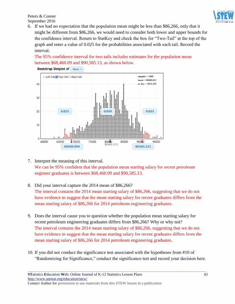
Peters & Conner

September 2016

_____________________________________________________________________________________________




6. If we had no expectation that the population mean might be less than $86,266, only that it

might be different from $86,266, we would need to consider both lower and upper bounds for

the confidence interval. Return to StatKey and check the box for “Two-Tail” at the top of the

graph and enter a value of 0.025 for the probabilities associated with each tail. Record the

interval.

The 95% confidence interval for two tails includes estimates for the population mean

between $68,460.09 and $90,585.13, as shown below.


We can be 95% confident that the population mean starting salary for recent petroleum

engineer graduates is between $68,460.09 and $90,585.13.


The interval contains the 2014 mean starting salary of $86,266, suggesting that we do not

have evidence to suggest that the mean starting salary for recent graduates differs from the

mean starting salary of $86,266 for 2014 petroleum engineering graduates.


recent petroleum engineering graduates differs from $86,266? Why or why not?

The interval contains the 2014 mean starting salary of $86,266, suggesting that we do not

have evidence to suggest that the mean starting salary for recent graduates differs from the

mean starting salary of $86,266 for 2014 petroleum engineering graduates.

10. If you did not conduct the significance test associated with the hypotheses from #10 of

“Randomizing for Significance,” conduct the significance test and record your decision here.


Peters & Conner

September 2016

_____________________________________________________________________________________________




The probability of obtaining a mean starting salary equal to the original sample mean of

$80,603.06 or more extreme than the sample mean if the null hypothesis is true is greater

than 5% because the sample mean does not fall in either tail of the randomization

distribution. Therefore, we would fail to reject the null hypothesis and conclude that we do

not have sufficient evidence to suggest that the mean starting salary for recent graduates

differs from the mean starting salary of $86,266 for 2014 petroleum engineering graduates.

11. How does this decision compare with the conclusion you drew from the confidence interval?

The conclusions are the same.

12. Use your comparison of conclusions between significance tests and confidence intervals in

#5 and #11 to draw a conjecture about the relationship between significance tests and

confidence intervals.

In general, if a one-sided significance test yields significant results at the level of , then the

one-sided (100 - )% confidence interval should not capture the hypothesized parameter

value. If a one-sided significance test does not yield significant results at the level of , then

the one-sided (100 - )% confidence interval should capture the hypothesized parameter

value. If a two-sided significance test yields significant results at the level of , then the two-

sided (100 - )% confidence interval should not capture the hypothesized parameter value. If

a two-sided significance test does not yield significant results at the level of , then the two-

sided (100 - )% confidence interval should capture the hypothesized parameter value.

Try This on your Own

1. Record your null and alternative hypotheses for the test you will perform.

𝐻0: 𝑝 = 0.845

𝐻1: 𝑝 < 0.845

2. Use StatKey to perform the simulation efficiently.

a. From the main StatKey menu, select “Test for Single Proportion” from the

“Randomization Hypothesis Test” options.

b. Click to “Edit Data,” and enter the appropriate count of graduates who are employed for a

sample of size 250 consistent with the null hypothesis.

c. Enter the value for your null hypothesis proportion.

d. Generate 1000 samples.

e. Select the proper tail based on your alternative hypothesis, and use a significance level of

= 0.05.

Locate the sample proportion within the randomization distribution. Does it fall in the left

tail, the right tail, or in the middle of the randomization distribution?


Peters & Conner

September 2016

_____________________________________________________________________________________________




Sample randomization distribution:

Note that the sample proportion of 0.64 is below the left-tail boundary value of 0.808

displayed on the number line, so the sample proportion value of 0.64 falls in the left tail.

3. Are there many randomization sample proportions that are less than or equal to the original

sample proportion?

No—there are no sample proportions equal to or less than 0.64 displayed for the simulation

results displayed in #2.

4. In terms of your hypotheses, should you reject the null hypothesis in favor of the alternative

hypothesis or fail to reject the null hypothesis?

Reject the null hypothesis and accept the alternative hypothesis that we have evidence to

suggest that the population proportion of recent petroleum engineering graduates who obtain

employment is less than 84.5%.


employment rate for recent petroleum engineering graduates in relation to the employment

rate for 2014 graduates?

We have evidence to suggest that the employment rate for the population of recent petroleum

engineering graduates is less than 84.5%.

6. Use StatKey to find a 95% confidence interval for the population proportion employment

rate for recent petroleum engineering graduates.

a. From the main StatKey menu, select “CI for Single Proportion” from the “Bootstrap


b. You may need to click on “Edit Data,” and enter the count of 160 for the count of

graduates who are employed and the sample of size 250.



Peters & Conner

September 2016

_____________________________________________________________________________________________




d. Check the appropriate box for “Left Tail,” “Two-Tail,” or “Right Tail” at the top of the

graph and enter the probability associated with that option. Record the interval.

Sample bootstrap distribution:


Using the bootstrap distribution, we can be 95% confident that the population proportion of

recent petroleum engineering graduates who are employed is less than 69%.

8. Did your interval capture the 2014 employment rate of 84.5%? No.

9. Does the interval cause you to question whether the population proportion for recent

petroleum engineering graduates’ employment is less than 84.5%? Why or why not?

Yes—because the hypothesized proportion of 84.5% was not captured by the confidence

interval, which consisted entirely of values that are less than 84.5%, we have evidence to

suggest that the real population proportion of recent petroleum engineering graduates who

obtain employment is less than 84.5%.

10. Recall your decision for the significance test you conducted and that you recorded in #4.

How does the decision compare with the conclusion you drew from the confidence interval?

In both cases, we have evidence to suggest that the population proportion of recent petroleum

engineering graduates who obtain employment is less than 84.5%.

11. Did your conjecture for the relationship between significance tests and confidence intervals

hold? If not, make a new conjecture.

In general, if a one-sided significance test yields significant results at the level of , then the

one-sided (100 - )% confidence interval should not capture the hypothesized parameter

value. If a one-sided significance test does not yield significant results at the level of , then

the one-sided (100 - )% confidence interval should capture the hypothesized parameter

value. If a two-sided significance test yields significant results at the level of , then the two-

sided (100 - )% confidence interval should not capture the hypothesized parameter value. If

a two-sided significance test does not yield significant results at the level of , then the two-

sided (100 - )% confidence interval should capture the hypothesized parameter value.


Documents

MORE CONFIDENCE IN SALARIES IN PETROLEUM ENGINEERING · MORE CONFIDENCE IN SALARIES IN PETROLEUM ENGINEERING ... Petroleum Engineering”, then you can skip Part 1 and only complete