Moral Geosta IJC 2010

INTERNATIONAL JOURNAL OF CLIMATOLOGYInt. J. Climatol. 30: 620–631 (2010)Published online 9 April 2009 in Wiley InterScience(www.interscience.wiley.com) DOI: 10.1002/joc.1913

Comparison of different geostatistical approaches to mapclimate variables: application to precipitation

Francisco J. Moral*Department of Graphic Representation, University of Extremadura, 06071 Badajoz, Spain

ABSTRACT: The benefits of an integrated geographical information system (GIS) and a geostatistics approach to accuratelymodel the spatial distribution pattern of precipitation are known. However, the determination of the most appropriategeostatistical algorithm for each case is usually neglected, i.e. it is important to select the best interpolation techniquefor each study area to obtain accurate results. In this work, the ordinary kriging (OK), simple kriging (SK) and universalkriging (universal kriging) methods are compared with three multivariate algorithms which take into account the altitude:collocated ordinary cokriging (OCK), simple kriging with varying local means (SKV) and regression-kriging (RK). Thedifferent techniques are applied to monthly and annual precipitation data measured at 136 meteorological stations in aregion of southwestern Spain (Extremadura). After carrying out cross-validation, the smallest prediction errors are obtainedfor the three multivariate algorithms but, particularly, SKV and RK outperform collocated OCK, which needs a moredemanding variogram analysis. These algorithms are easily implemented in a GIS, requiring the residual estimates andmap algebra capability to generate the final maps. Results evidence the necessity of accounting for spatially dependentprecipitation data and the collocated altitude, to accurately define monthly and annual precipitation maps. Copyright 2009 Royal Meteorological Society

KEY WORDS kriging; precipitation; altitude; geographical information system; regression

Received 11 July 2008; Revised 22 January 2009; Accepted 8 March 2009

1. Introduction

There are many different areas of research (e.g. climatol-ogy, agriculture, ecological modelling, hydrology) thatrequire interpolated surfaces or gridded datasets of cli-mate variables. Consequently, there have been numerousattempts made at spatial interpolation using a variety ofmethods.

Surfaces of climate variables have been interpolated,using point data, for areas ranging from a few thou-sand square kilometres (Ninyerola et al., 2000; Vicente-Serrano et al., 2003) to the continental scale (Hulmeet al., 1995, 1996) and even for the entire globe (Willmottand Robeson, 1995).

The main problem, previous to the selection of themost appropriate estimation technique, is related tothe availability of climatic data. Sometimes data arerecorded at permanent but too much disperse weatherstations, especially in mountainous areas, where climaticvalues are more difficult to predict due to the complextopography. Even in flatter areas, weather stations shouldbe properly distributed to detect the influences of airflows, surrounding mountains, thermal inversions andother phenomena that could affect the climatic patterns.

* Correspondence to: Francisco J. Moral, Department of Graphic Rep-resentation, University of Extremadura, 06071 Badajoz, Spain.E-mail: [email protected]

The spatial interpolation methods differ in theirassumptions, deterministic or statistical nature, and local(they use the data of the nearest sampling points toestimate at unsampled locations) or global (they usethe data of all sampling points to estimate at unsam-pled sites) perspective (Burrough and McDonnell, 1998).Some examples related to the use of deterministic tech-niques can be found in the works of Legates andWillmott (1990) – inverse distance weighting; Hutchin-son and Gessler (1994) – splines; Agnew and Palutikof(2000) or Vicente-Serrano et al. (2003) – empirical mul-tiple regressions. However, it is recognized that the statis-tical approach, geostatistical methods or kriging, has sev-eral advantages over the deterministic techniques (Isaaksand Srivastava, 1989; Goovaerts, 1997). Nowadays, geo-statistics is widely used in climate mapping (Atkinson,1997; Goovaerts, 1997). The fact of giving unbiased pre-dictions with minimum variance and taking into accountthe spatial correlation between the data recorded at differ-ent weather stations is an important advantage of kriging.

Some studies have shown that kriging provides bet-ter estimates than other techniques (e.g. Phillips et al.,1992; Goovaerts, 2000), but other authors have foundthat results depend on the sampling density (Dirks et al.,1998). A major advantage of kriging over simpler meth-ods, besides providing a measure of prediction error(kriging variance), is the possibility of complementingthe sample data, when they are sparse, by secondary orauxiliary information which can help with interpolation.

Copyright 2009 Royal Meteorological Society

DIFFERENT GEOSTATISTICAL APPROACHES TO MAP CLIMATE VARIABLES 621

Those sources of knowledge are: (1) data from a cheap-to-measure covariable which is known at many morepoints, and (2) an empirical spatial model of a drivingprocess.

For precipitation, weather–radar observations can bethe secondary data, as Azimi-Zonooz et al. (1989) andRaspa et al. (1997) considered to estimate precipitationfields using multivariate extensions of kriging (cokrigingand kriging with an external drift, respectively). How-ever, Goovaerts (2000) suggested the use of altitude froma digital elevation model (DEM) as another valuable andcheaper source of auxiliary data. It is known that pre-cipitation is higher with increasing elevation, due to theorographic effect of mountainous areas where the air islifted vertically and the condensation generates becauseof adiabatic cooling. Goovaerts (2000) showed that geo-statistical algorithms outperform deterministic techniquesand, especially, multivariate extensions of kriging, wherethe altitude is considered, generate the best results. Morerecently, Diodato (2005) also found better estimates whenordinary cokriging (OCK), considering altitude as theauxiliary data, is compared with ordinary kriging (OK).

During the last years, some mixed interpolation tech-niques have been developed, combining kriging and thesecondary information. According to Hengl et al. (2003),these methods can be classified depending on the prop-erties of input data. When the number of secondary vari-ables is low and these auxiliary data are not availableat all grid-nodes, cokriging is the most appropriate inter-polation technique. If auxiliary data are available at allgrid-nodes and correlated with the primary or target vari-able, kriging with a trend model or external drift (Hudsonand Wackernagel, 1994; Bourennane et al., 2000) is thecorrect interpolation method. This non-stationary geosta-tistical technique has three different approaches from acomputational point of view. In the first, called univer-sal kriging (UK), the trend is modelled as a functionof coordinates (Deutsch and Journel, 1992; Wackernagel,1998). If the trend is defined externally, with some sec-ondary variables, the term kriging with external drift (ortrend) is used (Wackernagel, 1998; Chiles and Delfiner,1999). The third approach consists in a regression mod-elling; the trend is modelled outside the kriging algo-rithm, followed by kriging of residuals. This was calledregression-kriging (RK) by Odeh et al. (1994, 1995),while Goovaerts (1999) employed the term kriging afterdetrending.

Another multivariate extension of kriging is the simplekriging (SK) with varying local means algorithm. In fact,it is similar to the kriging with external drift method, buthas some advantages over it (Goovaerts, 1997).

Besides the previously cited references, there aresome others about the use of different geostatisticaltechniques to interpolate precipitation data. Martınez-Cob (1996) obtained the best estimates using cokriging,including topography to improve predictions. Pardo-Iguzquiza (1998) found the best results for the predictionof precipitation by means of kriging with an externaldrift. However, according to Goovaerts (1999), RK has

proven to be superior to simpler geostatistical methods.Therefore, several methods must be compared to establishthe best technique to estimate precipitation in a particulararea or region. More unanimity exists when deterministicand geostatistical algorithms are compared. The greatmajority of works shows better results when kriging, orany multivariate extension of it, is used.

There are also some references about modelling clima-tological variables using geographical information sys-tems (GIS). For example, Ninyerola et al. (2000) andAgnew and Palutikof (2000) integrate statistical and GIStechniques to make climatic maps. The linkage of GIS,statistics and geostatistics provides a complementary setof tools for spatial analysis (Burrough, 2001).

In this paper, monthly and annual precipitation datafrom the Extremadura region (Spain) are interpolated togenerate high-resolution maps, using two types of geo-statistical methods: (1) algorithms that use only precipi-tation data recorded at the meteorological stations (ordi-nary kriging, OK and simple kriging, SK); (2) algorithmsthat combine precipitation data with auxiliary informa-tion (universal kriging, UK; ordinary cokriging, OCK;simple kriging, SK with varying local means, SKV; andregression-kriging, RK). Prediction performances of thealgorithms are compared using cross-validation and theone with higher accuracy of estimates is selected to mapprecipitation. Thirteen maps were the outcome of thiswork: 12 maps of mean monthly precipitation and 1 ofmean annual precipitation. Investigation of the reasonsfor different performance between approaches is also car-ried out.

2. Site description

This work is centred in Extremadura (latitude between37°57′ and 40°29′ N, longitude between 4°39′ and7°33′ W). The region is located in the southwest ofSpain on the Portuguese border. It is one of the largestregions in Europe, with a surface area of approximately41 600 km2, the size of Belgium. Extremadura shows agreat contrast, with wide agricultural and forest areas, andis considered to be one of the most important ecologicalenclaves in Europe. In the north lie districts with gentlewooded hills, the Sierra de Gata and Hurdes, that throughthe fertile valleys of the Alagon, Jerte and La Vera, linkwith the high Gredos mountains. In the east lie the irriga-tion lands of the river Tagus, the rugged Villuercas, andthe areas of Los Montes and La Serena, with the longestinterior coast in the Iberian Peninsula, that descend fur-ther to the south, to the agricultural areas of La Campina.In the west the great plains of Brozas and Alcantara dropto the San Pedro mountains and lead into the rich plain ofthe Guadiana river. In the south lie the great pasture landsand the mountains of Jerez, Tentudıa and Hornachos.

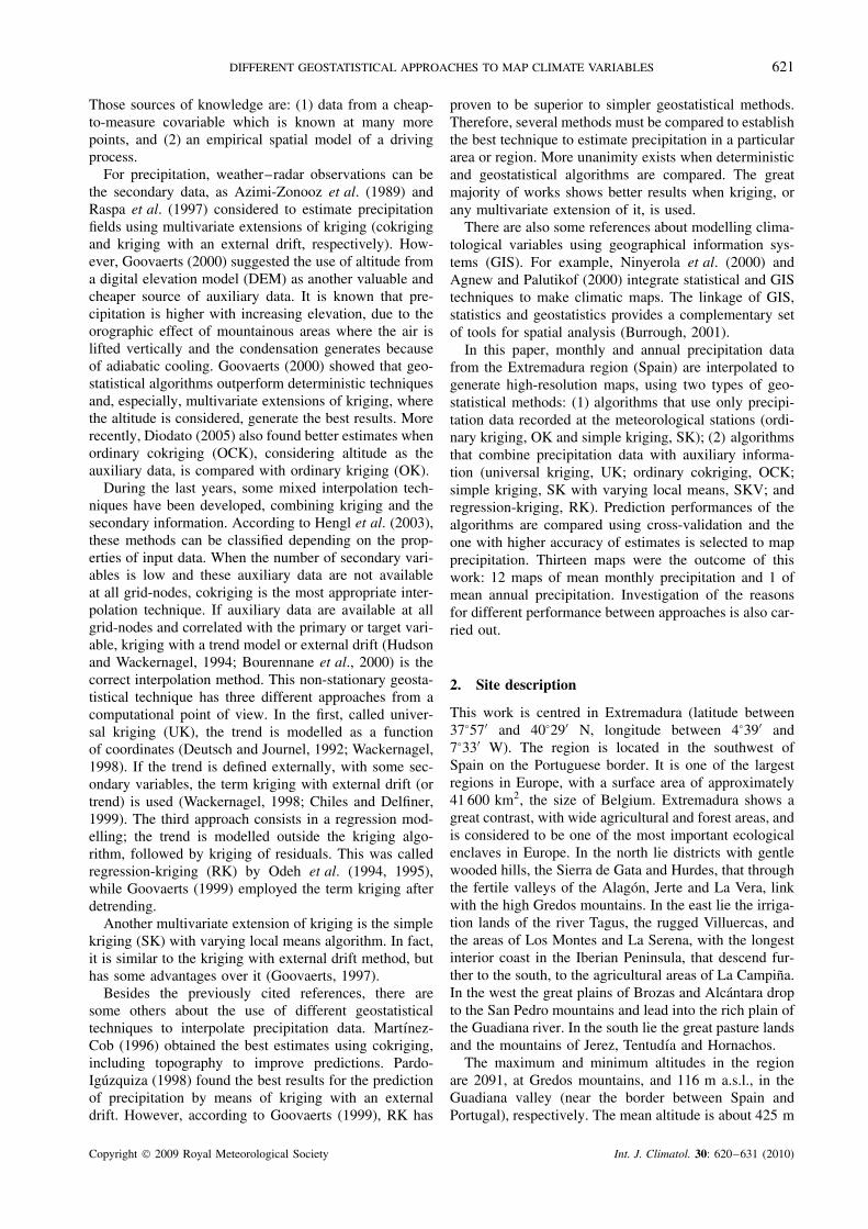
The maximum and minimum altitudes in the regionare 2091, at Gredos mountains, and 116 m a.s.l., in theGuadiana valley (near the border between Spain andPortugal), respectively. The mean altitude is about 425 m

Copyright 2009 Royal Meteorological Society Int. J. Climatol. 30: 620–631 (2010)

622 F. J. MORAL

Figure 1. Location and topography of the study area.

a.s.l. Figure 1 shows the DEM, with a spatial resolutionof 1 km, used in this research.

The climate of Extremadura is characterized by avariation in both temperature and precipitation typicalof a Mediterranean climate. However, this feature ismodified by the interior location of the region and byoceanic influences that penetrate the peninsula due to itsproximity to the Atlantic.

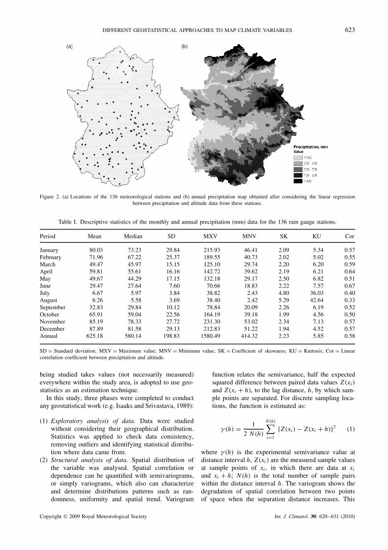
Mean annual precipitation reaches <600 mm in themajority of the areas of the region, even <400 mmin the centre of the Guadiana valley, but it can reachmuch >1000 mm in the northern (Gredos) and eastern(Guadalupe) mountainous areas. One of the most impor-tant characteristics of the precipitation is its interannualvariability. There are a dry season, from June to Septem-ber, and a wet season, from October to May (80% ofthe precipitation falls between these months). Periodicaldroughts with duration of 2 or more years, with an occur-rence of once in the 8–9 years, are frequent (Almarza,1984). Extremadura is a semiarid region, where the waterbalance is negative.

3. Material and methods

3.1. Data

Although active meteorological stations are numerous inExtremadura, daily data of precipitation were obtainedfrom those with series of more than 40 years, at leastbetween 1961 and 2000. Thus, the final spatial databasecontains 136 precipitation stations, which were geograph-ically referenced at UTM coordinates. The World Mete-orological Organization (WMO) gives 30 years as theoptimal length for a series with the aim of obtainingreliable climate data to make predictions (WMO, 1967).

Figure 2 shows the spatial distribution of the weatherstations used in this work. It should be indicated thatlocations of the stations are not the ideal. There areconsiderable spatial variations in certain areas. Manystations are placed in flat areas, so that they are lackingin the mountainous areas. But, even in some flat areas,stations are unevenly distributed.

The daily observations made at all stations havepassed through a rigorous quality control procedure.Consistency checks were applied to data and, of course,climatological data from series within 40 years werefiltered out, to avoid possible errors during the analysis ofthe information. We were very strict with data selection,only keeping weather stations with complete years. Afterassuring the raw data quality, monthly precipitationaverages were calculated. This information was loaded tothe spatial database and used as the source of input datafor the gridding process. Some basic sample statisticswere also determined (Table I). Fluctuations of monthlyand annual precipitations from one year to another werenot investigated.

The elevation data is another source of information.Altitude of each meteorological station was included inthe spatial database. This auxiliary information can helpto improve the estimates of precipitation.

3.2. Geostatistical interpolation techniques

In this section, the estimators used in the case study arebriefly introduced. More information about them can befound in, for instance, Isaaks and Srivastava (1989) andGoovaerts (1997).

Each precipitation datum is regarded as one drawn atrandom according to some law, from some probabilitydistribution. This point of view, when the studied vari-able (precipitation) is considered random and distributedcontinuously (regionalized variable), i.e. the phenomenon



Figure 2. (a) Locations of the 136 meteorological stations and (b) annual precipitation map obtained after considering the linear regressionbetween precipitation and altitude data from these stations.

Table I. Descriptive statistics of the monthly and annual precipitation (mm) data for the 136 rain gauge stations.

Period Mean Median SD MXV MNV SK KU Cor

January 80.03 73.23 29.84 215.93 46.41 2.09 5.34 0.57February 71.96 67.22 25.37 189.55 40.73 2.02 5.02 0.55March 49.47 45.97 15.15 125.10 29.74 2.20 6.20 0.59April 59.81 55.61 16.16 142.72 39.62 2.19 6.21 0.64May 49.67 44.29 17.15 132.18 29.17 2.50 6.82 0.51June 29.47 27.64 7.60 70.66 18.83 2.22 7.57 0.67July 6.67 5.97 3.84 38.82 2.43 4.80 36.03 0.40August 6.26 5.58 3.69 38.40 2.42 5.29 42.64 0.33September 32.83 29.84 10.12 78.84 20.09 2.26 6.19 0.52October 65.91 59.04 22.56 164.19 39.18 1.99 4.56 0.50November 85.19 78.33 27.72 231.30 53.02 2.34 7.13 0.57December 87.89 81.58 29.13 212.83 51.22 1.94 4.52 0.57Annual 625.18 580.14 198.83 1580.49 414.32 2.23 5.85 0.58

SD = Standard deviation; MXV = Maximum value; MNV = Minimum value; SK = Coefficient of skewness; KU = Kurtosis; Cor = Linearcorrelation coefficient between precipitation and altitude.

being studied takes values (not necessarily measured)everywhere within the study area, is adopted to use geo-statistics as an estimation technique.

In this study, three phases were completed to conductany geostatistical work (e.g. Isaaks and Srivastava, 1989):

(1) Exploratory analysis of data. Data were studiedwithout considering their geographical distribution.Statistics was applied to check data consistency,removing outliers and identifying statistical distribu-tion where data came from.

(2) Structural analysis of data. Spatial distribution ofthe variable was analysed. Spatial correlation ordependence can be quantified with semivariograms,or simply variograms, which also can characterizeand determine distributions patterns such as ran-domness, uniformity and spatial trend. Variogram

function relates the semivariance, half the expectedsquared difference between paired data values Z(xi)

and Z(xi + h), to the lag distance, h, by which sam-ple points are separated. For discrete sampling loca-tions, the function is estimated as:

γ (h) = 1

2 N(h)

N(h)∑

i=1

{Z(xi) − Z(xi + h)}2 (1)

where γ (h) is the experimental semivariance value atdistance interval h, Z(xi) are the measured sample valuesat sample points of xi , in which there are data at xi

and xi + h; N(h) is the total number of sample pairswithin the distance interval h. The variogram shows thedegradation of spatial correlation between two pointsof space when the separation distance increases. This


624 F. J. MORAL

function has two components: (i) the nugget effect, whichcharacterize the discontinuity jump observed at the originof distances, quantifies the short-term, erratic variationsof the studied phenomenon plus measurements and dataerrors; (ii) the increasing part of the variogram, whichmay reach the sill (theoretical sample variance), levellingoff the curve, for a distance called range, or keep onincreasing continuously with distance. The non-nuggetpart of the variogram measures the non-random part ofthe phenomenon and models its average medium-scalebehaviour in space.

The variogram is a function of both the distanceand direction, and so direction-dependent variability canbe accounted for. Because of the lack of data onlythe omnidirectional variograms were computed in thisstudy. Therefore, the spatial variability is assumed to beidentical in all directions.

When an experimental variogram is defined, i.e. somepoints of a variogram plot are determined by calculatingvariogram at different lags, a model (theoretical vari-ogram) should be fitted to the points. Although there aresome statistical techniques to justify the choice of a theo-retical variogram (Cressie, 1985), subjective criteria andprevious experiences are the main tools to choose one.(3) Predictions. Geostatistics offers a great variety of

methods that provide estimates for unsampled loca-tions. These methods are known as kriging, inhonour of Danie Krige, who first formulated thisform of interpolation in 1951 (Krige, 1951). Krig-ing is regarded as the best linear unbiased estimator(BLUE). Weights for sample values are calculatedbased on the parameters of the variogram model.

All geostatistical estimators are variants of the linearregression estimator Z∗(x):

Z∗(x) − m(x) =n∑

i=1

wi(x) · [Z(xi) − m(xi)] (2)

where each datum, Z(xi), has an associated weight,wi(x), and, m(x) and m(xi) are the expected valuesof Z∗(x) and Z(xi), respectively. The kriging weightsmust be determined to minimize the estimation variance,Var[Z∗(x) − Z(x)], while ensuring the unbiasedness ofthe estimator, E[Z∗(x) − Z(x)] = 0.

All different types of kriging are distinguished depend-ing on the chosen model for the trend, m(x), of therandom function Z(x) (e.g. Goovaerts, 1997). Thus, SKconsiders m(x) to be known and constant, m, all overthe study area; unlike the previous kriging type, m(x) isunknown in the OK and is considered to fluctuate locally,maintaining the stationarity within the local neighbour-hood; UK considers that m(x) smoothly varies withineach local neighbourhood and is modelled as a linearcombination of functions of the spatial coordinates.

The weights, wi(x), are generated when the corre-sponding system of linear equations, depending on thetype of kriging, is solved [see Isaaks and Srivastava

(1989) or Goovaerts (1997) for a detailed presentationof the kriging algorithms].

Univariate algorithms, OK and SK, consider the prob-lem of estimating the precipitation at an unsampled loca-tion using only precipitation data. When UK is taking intoaccount, a previous model of the trend, function of thespatial coordinates, have to be selected. If auxiliary infor-mation, mainly altitude data, is considered together withthe primary data, precipitation, some multivariate exten-sion of kriging can result in better estimates. In this case,the simplest approach is using a linear relation betweenthe precipitation and the collocated altitude:

Z∗(x) = a + bH(x) (3)

where the two regression coefficients, a and b, are esti-mated from the set of collocated precipitation and altitudedata, Z(xi) and H(xi), respectively. Using map algebratechniques, all cells of the raster DEM were multipliedby the corresponding regression coefficient, b, and later,the interception value, a, was added. With this method,the so-called regression maps were obtained (Figure 2).This methodology has been applied in some works (e.g.Vicente-Serrano et al., 2003). However, from a spatialpoint of view, the linear regression is an inexact interpo-lator. Only with the addition of the estimated residualsat each point an exact interpolator can be obtained, i.e.estimated values at each sample point (meteorologicalstation) are the same that observed values.

In mountainous areas, with sparse rainfall measure-ments, regressions may capture the orographic effect onprecipitation distribution, generating the best estimates(e.g. Daly et al., 1994), but if the spatial correlation ofthe precipitation data is taking into account, estimates areimproved (e.g. Guan et al., 2005).

SKV accounts for the secondary data replacing theknown stationary mean, m, by known varying means,mSKV(x), which are usually relations similar to (3). Inthis case, the weights, wi(x) are generated by solving aSK system where the covariance function of the residuals[r(x) = Z(x) − mSKV(x)] is involved (Goovaerts, 1997).The estimate at a location x, Z∗

SKV(x), is:

Z∗SKV(x) = f (H(x)) +

n∑

i=1

wi(x) r(xi) (4)

where f (H(x)) is the regression estimate.There is an alternative approach to use the secondary

data and perform SK on the corresponding residuals:kriging with an external drift, KE. This is but a variantof UK. The trend is modelled as a linear function ofthe auxiliary information, instead of as a function ofthe coordinates. The KE estimator is similar to the SKVestimator. However, the definition of the trend is differentin both methods: whereas the trend coefficients, a and b,are unique and generated without considering the krigingsystem in the SKV approach, these coefficients areimplicitly estimated within each search neighbourhood



by the kriging system in the KE algorithm. Thus, KEextrapolates the linear trend model to the last data, whichcould be unrealistic sometimes. SKV is more robust inthat it extrapolates a relation that is fitted to all data (amore exhaustive discussion can be found in Goovaerts,1997). This is the reason why the KE algorithm was notemployed in this study.

The cokriging approach is another possibility to incor-porate secondary data. Although it is indicated when thesecondary information is not exhaustive, i.e. auxiliarydata are not available at all grid-nodes, if this informa-tion is known everywhere and changes smoothly acrossthe study area, the cokriging system can retain only thesecondary datum collocated with the location which isestimated (Goovaerts, 1997). The collocated cokrigingestimate, Z∗

CK(x), is:

Z∗CK(x) =

n∑

i=1

wi(x) · Z(xi) + wn+1

[H(x) − m2 + m1] (5)

where m1 and m2 are the global means of the precipitationand altitude data, respectively. The weights, wi(x) andwn+1, are solutions of the cokriging system. Now, it isnecessary to calculate and model one variogram for theprecipitation data, another one for the altitude and theircross variogram, which is computed as:

γ (h) = 1

2 N(h)

N(h)∑

i=1{[Z(xi) − Z(xi + h)][H(xi) − H(xi + h]

}(6)

Altitude data is considered in a different way whencokriging and SKV are compared. Whereas altitudedatum provides information about the trend in the SKVapproach, the cokriging estimate is directly influencedby it. If the same assumptions about the mean in theOK approach are considered, similarly to that, the OCK,method is defined.

When RK is used, predictions are made separately forthe trend and residuals and then added back together.Thus, the precipitation at a new unsampled point, x, isestimated using RK as follows:

Z∗RK(x) = m(x) + r(x) (7)

where the trend, m(x), is fitted using linear regressionanalysis and the residuals, r(x), are estimated using OK.If cj are the coefficients of the estimated trend model,vj (x) is the jth predictor at location x, p is the number ofpredictors, wi(x) are the weights determined by solvingthe OK system of the regression residuals, r(xi), for then sample points, the prediction, Z∗

RK(x), is made by:

Z∗RK(x) =

p∑

j=0

cj · vj (x) +n∑

i=1

wi(x) · r(xi)

v0(x) = 1 (8)

The trend model coefficients can be solved using aweighted linear regression, where the covariance matrix,i.e. covariances between sample point pairs, is employedas the matrix of weights (Cressie, 1993, p.166). If thereis no significant spatial clustering between sample points,regression coefficients using an ordinary least squareestimation are similar than those obtained with a generalleast square estimation based on the spatial matrix ofresiduals.

According to Goovaerts (1997), before applying RKtwo general requirements need to be fulfilled: (1) relationbetween the target and predictors must be linear,(2) value of predictors must be known at all primary datalocations and all new locations where the predictions aremade.

The choice of independent variables to model thetrend should be based on the most known factors thatinfluence on the precipitation. One of the most importantis the altitude (e.g. Agnew and Palutikof, 2000), H .In this study, it is the only one predictor used. H isthe nominal altitude, in metres, of the stations, derivedfrom the 1 km resolution DEM. It generates informationabout the variability due to the relief. Although theremay be potential for improving the predictions, e.g.by including further factors, only H was consideredto compare RK estimates with the other multivariateextensions of kriging.

All geostatistical analyses were conducted using theextension Geostatistical Analystd of the GIS softwareArcGISd (version 9.1, ESRI Inc, Redlands California,USA). After modelling the annual and monthly precipi-tation with the selected algorithms, a set of map layersin raster format was generated. These layers were basedon grids, where each point (datum) represents the centerof a 1000 m side square. All maps were produced withthe ArcMapd module of the ArcGISd.

4. Results: assessment of the geostatisticalinterpolators

During the exploratory analysis of precipitation data, thefirst phase of any geostatistical study, data distributionwas described using classical descriptive statistics. It wasobserved that monthly and annual mean and median val-ues were appreciably different and, moreover, the coeffi-cients of skewness were high (Table I). After performingthe logarithmic transformation of the data, normality wasapparent, i.e. mean and median values were similar andthe coefficients of skewness were lower and nearer tozero (Table II). This means that monthly and annual pre-cipitation data fit to lognormal distributions. Althoughnormality is not a prerequisite for kriging, it is a desir-able property. Kriging will only generate the best absoluteestimate if the random function fits a normal distribution.

The correlations between precipitation and altitude foreach month and all year were analysed. Linear correlationcoefficients (Table I) ranging from 0.33 (August) to 0.67(June) indicate that the secondary data, altitude, can be


626 F. J. MORAL

Table II. Descriptive statistics of the monthly and annual precipitation (mm) data, transformed to their corresponding naturallogarithms, for the 136 rain gauge stations.

Period Mean Median SD MXV MNV SK KU CorL

January 4.33 4.29 0.31 5.38 3.84 1.04 4.03 0.55February 4.23 4.21 0.30 5.24 3.71 0.98 4.01 0.51March 3.87 3.83 0.26 4.83 3.39 1.18 4.76 0.56April 4.06 4.02 0.23 4.96 3.68 1.29 4.95 0.62May 3.86 3.79 0.27 4.88 3.37 1.59 5.65 0.48June 3.36 3.32 0.22 4.26 2.94 1.12 4.95 0.70July 1.80 1.79 0.41 3.66 0.89 0.86 5.22 0.44August 1.74 1.72 0.41 3.65 0.89 0.88 5.62 0.30September 3.46 3.40 0.26 4.37 3.00 1.27 5.00 0.50October 4.14 4.08 0.29 5.10 3.67 1.06 4.11 0.46November 4.41 4.36 0.27 5.44 3.97 1.25 4.92 0.55December 4.43 4.40 0.28 5.36 3.93 0.98 3.99 0.54Annual 6.40 6.36 0.26 7.37 6.03 1.29 4.81 0.56

SD = Standard deviation; MXV = Maximum value; MNV = Minimum value; SK = Coefficient of skewness; KU = Kurtosis; CorL = Linearcorrelation coefficient between natural logarithm of precipitation and altitude.

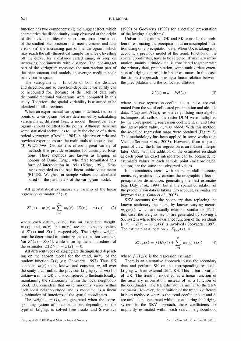
Figure 3. (a) Nugget effect, sill and (b) relative nugget effect values of the monthly and annual variograms for the precipitation data.

worth incorporating into the mapping of precipitation.Previous transformation of precipitation data using thenatural logarithm did not generate, in general, betterregressions (Table II), so it was not considered.

The structural analysis was carried out with the omnidi-rectional variogram. Experimental variograms were com-puted for monthly and annual data. The fact that twoprecipitation data close to each other are more alike thanthose that are further apart is apparent in the variogramvalues which increase with the separation distance. A lin-ear combination of two models, one spherical and one lin-eal, and a nugget effect, provided the best fit for all cases.This indicates that the spatial dependence occurs at twodifferent scales, which are represented in the variogramas two spatial components. The short-range component

is described by the spherical model and the long-rangecomponent by the linear model. Monthly and annual var-iograms have similar shape, due to the control of therelief on the spatial distribution of precipitation, althoughthe range and nugget effect fluctuate from one month toanother (Figure 3).

The choice of a particular variogram model is depen-dent upon the expected spatial variability. A variable likeprecipitation can be distributed erratically in reduced dis-tances and exponential or spherical models are the mostsuitable (Isaaks and Srivastava, 1989). Spatial depen-dence of the monthly precipitation data displayed somedifferences as determined by variogram analyses. Vari-ogram parameters varied between months. The nuggeteffect was estimated extending the variogram until the



vertical axis. The behaviour near the origin is very impor-tant because of the influence on the interpolation process.In this work, variograms showed a considerable nuggeteffect during the driest months, July and August, whenthe spatial variability of precipitation is higher at a scalesmaller than the minimum lag distance (Figure 3). How-ever, the relative nugget effect, ratio of the nugget dis-continuity to the sill value, has its maximum in May,remaining high from June to September, also the driestmonths (Figure 3). During this period, an important partof the variance is due to the nugget effect. The way ofdecreasing the high nugget effect is considering closerprecipitation data, which will only be possible in thefuture, when more information from new weather stationsis available. The sills (Figure 3) are depending on thesample variances. These results are in accordance withstandard deviations shown in Table II.

The linear model of the long-range component impliesthat if we were to increase the region surveyed we shouldencounter ever more variation. Probably, the sill of thelong-range scale is achieved for a distance greater thanthe limits of the experimental area.

The third phase of the geostatistical study, the predic-tion at all unsampled locations, was carried out usingunivariate and multivariate interpolators, which integratethe spatial correlation structures described with the vari-ograms.

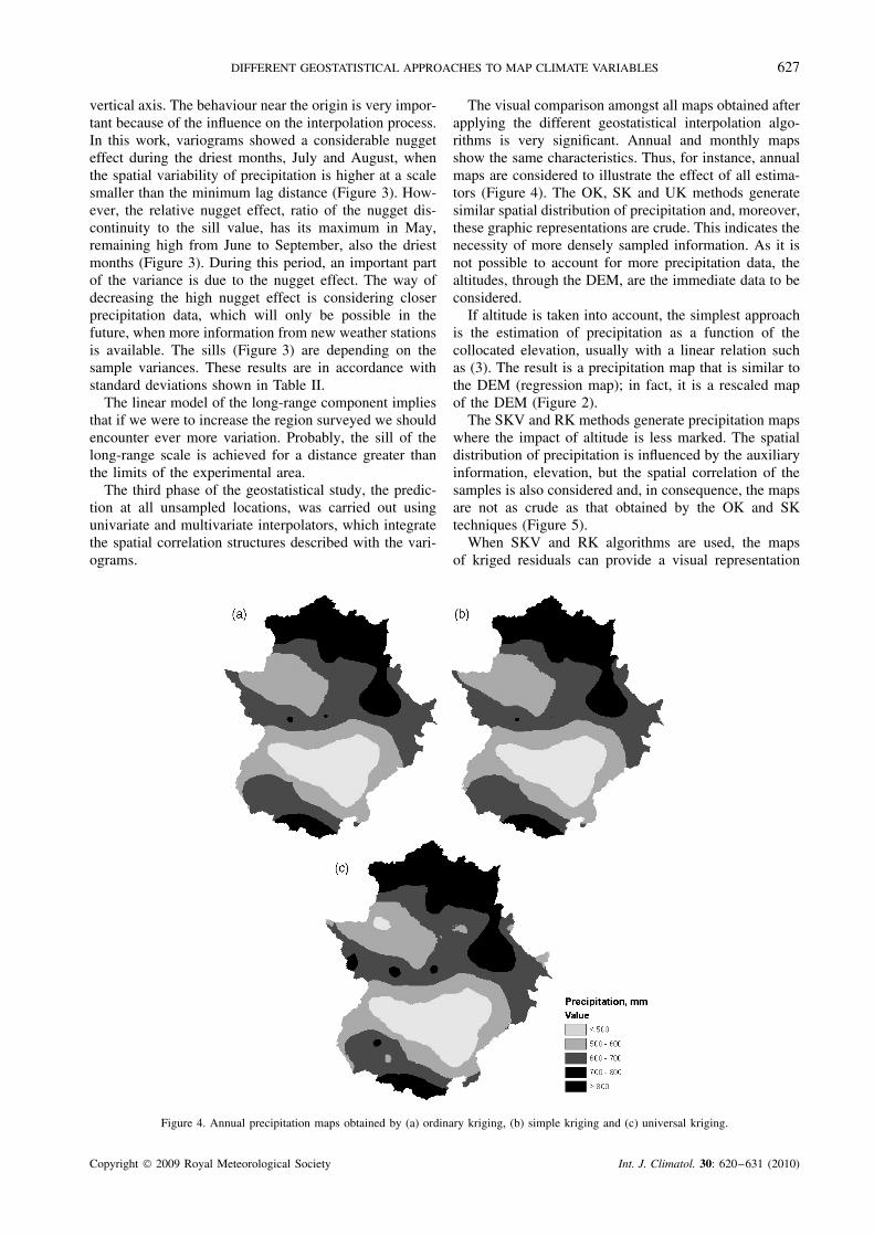
The visual comparison amongst all maps obtained afterapplying the different geostatistical interpolation algo-rithms is very significant. Annual and monthly mapsshow the same characteristics. Thus, for instance, annualmaps are considered to illustrate the effect of all estima-tors (Figure 4). The OK, SK and UK methods generatesimilar spatial distribution of precipitation and, moreover,these graphic representations are crude. This indicates thenecessity of more densely sampled information. As it isnot possible to account for more precipitation data, thealtitudes, through the DEM, are the immediate data to beconsidered.

If altitude is taken into account, the simplest approachis the estimation of precipitation as a function of thecollocated elevation, usually with a linear relation suchas (3). The result is a precipitation map that is similar tothe DEM (regression map); in fact, it is a rescaled mapof the DEM (Figure 2).

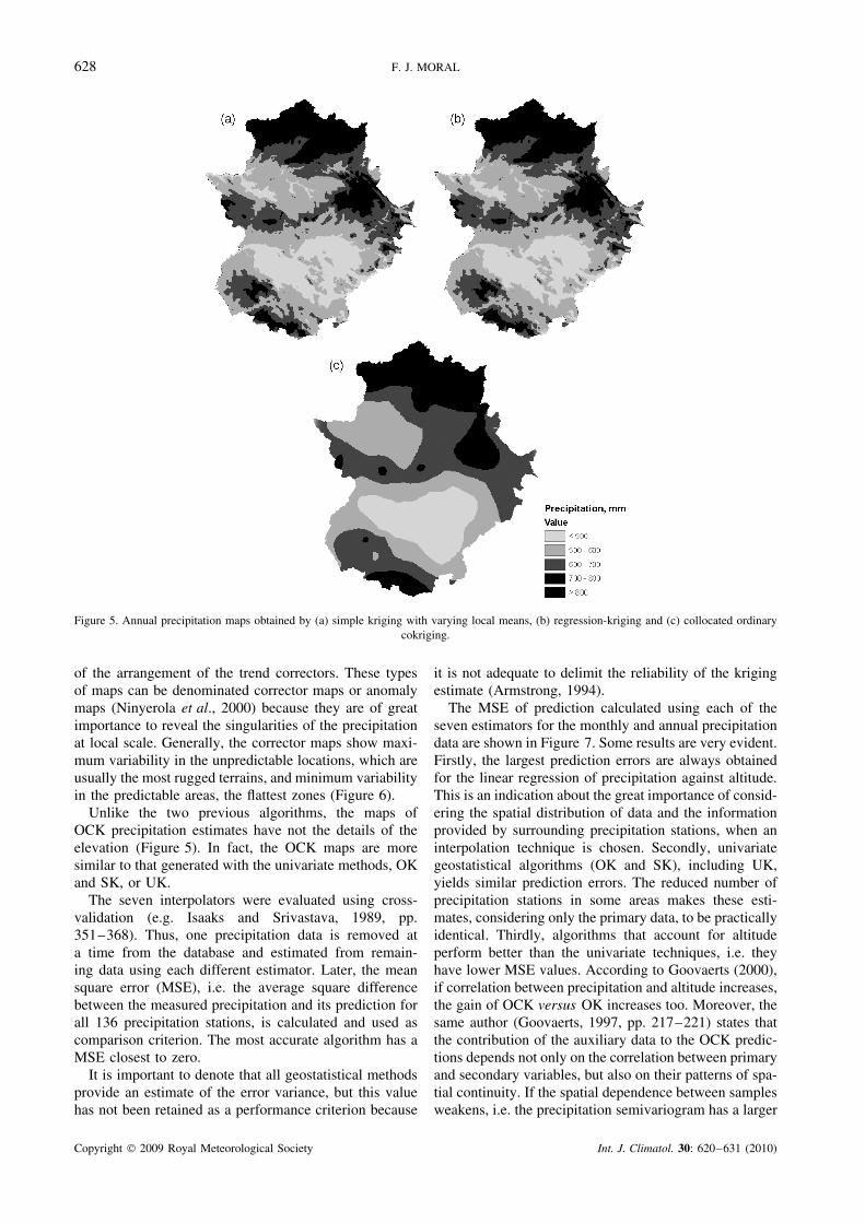
The SKV and RK methods generate precipitation mapswhere the impact of altitude is less marked. The spatialdistribution of precipitation is influenced by the auxiliaryinformation, elevation, but the spatial correlation of thesamples is also considered and, in consequence, the mapsare not as crude as that obtained by the OK and SKtechniques (Figure 5).

When SKV and RK algorithms are used, the mapsof kriged residuals can provide a visual representation

Figure 4. Annual precipitation maps obtained by (a) ordinary kriging, (b) simple kriging and (c) universal kriging.


628 F. J. MORAL

Figure 5. Annual precipitation maps obtained by (a) simple kriging with varying local means, (b) regression-kriging and (c) collocated ordinarycokriging.

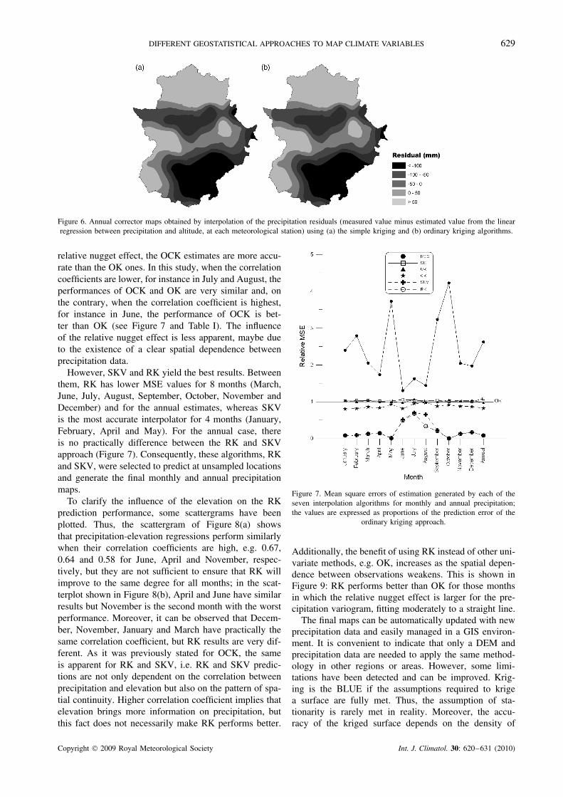
of the arrangement of the trend correctors. These typesof maps can be denominated corrector maps or anomalymaps (Ninyerola et al., 2000) because they are of greatimportance to reveal the singularities of the precipitationat local scale. Generally, the corrector maps show maxi-mum variability in the unpredictable locations, which areusually the most rugged terrains, and minimum variabilityin the predictable areas, the flattest zones (Figure 6).

Unlike the two previous algorithms, the maps ofOCK precipitation estimates have not the details of theelevation (Figure 5). In fact, the OCK maps are moresimilar to that generated with the univariate methods, OKand SK, or UK.

The seven interpolators were evaluated using cross-validation (e.g. Isaaks and Srivastava, 1989, pp.351–368). Thus, one precipitation data is removed ata time from the database and estimated from remain-ing data using each different estimator. Later, the meansquare error (MSE), i.e. the average square differencebetween the measured precipitation and its prediction forall 136 precipitation stations, is calculated and used ascomparison criterion. The most accurate algorithm has aMSE closest to zero.

It is important to denote that all geostatistical methodsprovide an estimate of the error variance, but this valuehas not been retained as a performance criterion because

it is not adequate to delimit the reliability of the krigingestimate (Armstrong, 1994).

The MSE of prediction calculated using each of theseven estimators for the monthly and annual precipitationdata are shown in Figure 7. Some results are very evident.Firstly, the largest prediction errors are always obtainedfor the linear regression of precipitation against altitude.This is an indication about the great importance of consid-ering the spatial distribution of data and the informationprovided by surrounding precipitation stations, when aninterpolation technique is chosen. Secondly, univariategeostatistical algorithms (OK and SK), including UK,yields similar prediction errors. The reduced number ofprecipitation stations in some areas makes these esti-mates, considering only the primary data, to be practicallyidentical. Thirdly, algorithms that account for altitudeperform better than the univariate techniques, i.e. theyhave lower MSE values. According to Goovaerts (2000),if correlation between precipitation and altitude increases,the gain of OCK versus OK increases too. Moreover, thesame author (Goovaerts, 1997, pp. 217–221) states thatthe contribution of the auxiliary data to the OCK predic-tions depends not only on the correlation between primaryand secondary variables, but also on their patterns of spa-tial continuity. If the spatial dependence between samplesweakens, i.e. the precipitation semivariogram has a larger



Figure 6. Annual corrector maps obtained by interpolation of the precipitation residuals (measured value minus estimated value from the linearregression between precipitation and altitude, at each meteorological station) using (a) the simple kriging and (b) ordinary kriging algorithms.

relative nugget effect, the OCK estimates are more accu-rate than the OK ones. In this study, when the correlationcoefficients are lower, for instance in July and August, theperformances of OCK and OK are very similar and, onthe contrary, when the correlation coefficient is highest,for instance in June, the performance of OCK is bet-ter than OK (see Figure 7 and Table I). The influenceof the relative nugget effect is less apparent, maybe dueto the existence of a clear spatial dependence betweenprecipitation data.

However, SKV and RK yield the best results. Betweenthem, RK has lower MSE values for 8 months (March,June, July, August, September, October, November andDecember) and for the annual estimates, whereas SKVis the most accurate interpolator for 4 months (January,February, April and May). For the annual case, thereis no practically difference between the RK and SKVapproach (Figure 7). Consequently, these algorithms, RKand SKV, were selected to predict at unsampled locationsand generate the final monthly and annual precipitationmaps.

To clarify the influence of the elevation on the RKprediction performance, some scattergrams have beenplotted. Thus, the scattergram of Figure 8(a) showsthat precipitation-elevation regressions perform similarlywhen their correlation coefficients are high, e.g. 0.67,0.64 and 0.58 for June, April and November, respec-tively, but they are not sufficient to ensure that RK willimprove to the same degree for all months; in the scat-terplot shown in Figure 8(b), April and June have similarresults but November is the second month with the worstperformance. Moreover, it can be observed that Decem-ber, November, January and March have practically thesame correlation coefficient, but RK results are very dif-ferent. As it was previously stated for OCK, the sameis apparent for RK and SKV, i.e. RK and SKV predic-tions are not only dependent on the correlation betweenprecipitation and elevation but also on the pattern of spa-tial continuity. Higher correlation coefficient implies thatelevation brings more information on precipitation, butthis fact does not necessarily make RK performs better.

Figure 7. Mean square errors of estimation generated by each of theseven interpolation algorithms for monthly and annual precipitation;the values are expressed as proportions of the prediction error of the

ordinary kriging approach.

Additionally, the benefit of using RK instead of other uni-variate methods, e.g. OK, increases as the spatial depen-dence between observations weakens. This is shown inFigure 9: RK performs better than OK for those monthsin which the relative nugget effect is larger for the pre-cipitation variogram, fitting moderately to a straight line.

The final maps can be automatically updated with newprecipitation data and easily managed in a GIS environ-ment. It is convenient to indicate that only a DEM andprecipitation data are needed to apply the same method-ology in other regions or areas. However, some limi-tations have been detected and can be improved. Krig-ing is the BLUE if the assumptions required to krigea surface are fully met. Thus, the assumption of sta-tionarity is rarely met in reality. Moreover, the accu-racy of the kriged surface depends on the density of


630 F. J. MORAL

Figure 8. Scattergrams between (a) the estimates using the precipitation-elevation regression and observations (correlation coefficients are 0.97,0.96 and 0.94 for June, April and November respectively) for some selected months, and between (b) the mean square error of prediction for

the regression-kriging approach and the correlation coefficients of precipitation-elevation regressions for all months.

Figure 9. Scattergram between the ratio of mean square error of prediction for the OK and RK techniques and the relative nugget effect valuesof the monthly and annual variograms for the precipitation data.

the network of meteorological stations. These problemsare partially overcome when SKV and RK are employedbecause the stationarity is replaced by known varyingmeans derived from the secondary data. Despite thelimitations outlined previously, a GIS-based approachhas important potential, given the range of topogra-phy, for instance, in the study area, Extremadura. Theresults of the cross-validation provide clear evidenceof the usefulness of kriging and the use of auxiliary

information, mainly altitude, in the spatial interpolationof precipitation.

Future research includes considering new indepen-dent variables, e.g. proximity to large bodies of waterand landcover, and the support of remote sensing.Using average synoptic circulation patterns as pre-dictors in the regression model, in addition to theterrain-based variables, can also contribute to refineestimates.



5. Conclusions

Highly accurate annual and monthly precipitation mapshave been generated by following a methodology thatcomprises geostatistical and GIS techniques. Univariateand multivariate geostatistical algorithms were appliedto estimate precipitation patterns from data recorded in136 meteorological stations in Extremadura region ofsouthwestern Spain. The results confirm other previousfindings (e.g. Goovaerts, 2000; Diodato, 2005) where, ingeneral, geostatistical algorithm interpolations are moreaccurate than predictions made using deterministic tech-niques. Moreover, if correlated secondary information,such as altitude, is considered, estimates can be furtherconsiderably improved. In this work, different geostatisti-cal methods to incorporate the secondary data have beenexamined. All multivariate techniques (OCK, SKV andRK) outperform univariate methods (OK, SK and UK)but, however, cross-validation has shown that predictionperformances vary among algorithms. SKV and RK pro-vide the smallest MSE of estimates and so performs betterthan the more demanding (three semivariograms have tobe modelled) OCK. The SKV and RK maps are influ-enced by the DEM pattern and show more details than thecokriged maps. Therefore, although these non-stationaryinterpolators have not been used extensively in clima-tology, they are potentially more appropriate to modelclimate variables than any form of cokriging.

Acknowledgements

The author thanks the reviewers of this paper for pro-viding constructive comments which have contributed toimprove the final version.

References

Agnew MD, Palutikof JP. 2000. GIS-based construction of baselineclimatologies for the Mediterranean using terrain variables. ClimateResearch 14: 115–127.

Almarza C. 1984. Fichas hıdricas normalizadas y otros parametroshidrometeorologicos, tomo II. National Meteorological InstituteINM: Madrid, Spain.

Atkinson PM. 1997. Geographical information science. Progress inPhysical Geography 21: 573–582.

Armstrong M. 1994. Is research in mining geostats as dead as adodo? In: Geostatistics for The Next Century, Dimitrakopoulos R(ed). Kluwer Academic: Dordrecht; 303–312.

Azimi-Zonooz A, Krajewski WF, Bowles DS, Seo DJ. 1989. Spatialrainfall estimation by linear and non-linear co-kriging of radar-rainfall and raingage data. Stochastic Hydrology and Hydraulics 3:51–67.

Burrough PA. 2001. GIS and geostatistics: essential partners for spatialanalysis. Environmental and Ecological Statistics 8: 361–377.

Burrough PA, McDonnell RA. 1998. Principles of GeographicalInformation Systems. Oxford University Press: Oxford.

Bourennane H, King D, Couturier A. 2000. Comparison of krigingwith external drift and simple linear regression for predictingsoil horizon thickness with different sample densities. Geoderma97(3–4): 255–271.

Chiles J, Delfiner P. 1999. Geostatistics: Modeling Spatial Uncertainty.John Wiley & Sons: New York.

Cressie N. 1985. Fitting variogram models by weighted least squares.Mathematical Geology 17(5): 563–586.

Cressie N. 1993. Statistics for Spatial Data. John Wiley & Sons: NewYork.

Daly C, Neilson RP, Phillips DL. 1994. A statistical topographic modelfor mapping climatological precipitation over mountain terrain.Journal of Applied Meteorology 33: 140–158.

Deutsch C, Journel A. 1992. Geostatistical Software Library andUser’s Guide. Oxford University Press: New York.

Diodato N. 2005. The influence of topographic co-variables on thespatial variability of precipitation over small regions of complexterrain. International Journal of Climatology 25: 351–363.

Dirks KN, Hay JE, Stow CD, Harris D. 1998. High-resolution studiesof rainfall on Norfolk Island, Part II: interpolation of rainfall data.Journal of Hydrology 208(3–4): 187–193.

Goovaerts P. 1997. Geostatistics for Natural Resources Evaluation.Oxford University Press: New York.

Goovaerts P. 1999. Using elevation to aid the geostatistical mappingof rainfall erosivity. Catena 34(3–4): 227–242.

Goovaerts P. 2000. Geostatistical approaches for incorporatingelevation into the spatial interpolation of rainfall. Journal ofHydrology 228: 113–129.

Guan H, Wilson JL, Makhnin O. 2005. Geostatistical mapping ofmountain precipitation incorporating auto-searched effects of terrainand climatic characteristics. Journal of Hydrometeorology 6(6):1018–1031.

Hengl T, Heuvelink GBM, Stein A. 2003. Comparison of kriging withexternal drift and regression-kriging. Technical Note, InternationalInstitute for Geo-information Science and Earth Observation (ITC),Enschede, http://www.itc.nl/library/Academic output..

Hudson G, Wackernagel H. 1994. Mapping temperature using krigingwith external drift: theory and an example from Scotland.International Journal of Climatology 14(1): 77–91.

Hulme M, Conway D, Jones PD, Jiang T, Barrow EM, Turney C.1995. Construction of a 1961–1990 European climatology forclimate change modelling and impact applications. InternationalJournal of Climatology 15: 1333–1363.

Hulme M, Conway D, Joyce A, Mulenga H. 1996. A 1961–90climatology for Africa south of the equator and a comparisonof potential evapotranspiration estimates. South Africa Journal ofScience 92(7): 334–343.

Hutchinson MF, Gessler PE. 1994. Splines – more than just a smoothinterpolator. Geoderma 62: 45–67.

Isaaks EH, Srivastava RM. 1989. An Introduction to AppliedGeostatistics. Oxford University Press: Oxford.

Krige DG. 1951. A statistical Approach to Some Mine Valuations andAllied Problems at the Witwatersrand. Master’s Thesis, Universityof Witwatersrand, South Africa.

Legates DR, Willmott CJ. 1990. Mean seasonal and spatial variabilityin global surface air temperature. Theoretical and AppliedClimatology 41: 11–21.

Martınez-Cob A. 1996. Multivariate geostatistical analysis ofevapotranspiration and precipitation in mountainous terrain. Journalof Hydrology 174: 19–35.

Ninyerola M, Pons X, Roure JM. 2000. A methodological approachof climatological modelling of air temperature and precipitationthrough GIS techniques. International Journal of Climatology 20:1823–1841.

Odeh I, McBratney A, Chittleborough D. 1994. Spatial prediction ofsoil properties from landform attributes derived from a digitalelevation model. Geoderma 63(3–4): 197–214.

Odeh I, McBratney A, Chittleborough D. 1995. Further results onprediction of soil properties from terrain attributes: heterotopiccokriging and regression-kriging. Geoderma 67(3–4): 215–226.

Pardo-Iguzquiza E. 1998. Comparison of geostatistical methods forestimating the areal average climatological rainfall mean usingdata of precipitation and topography. International Journal ofClimatology 18: 1031–1047.

Phillips DL, Dolph J, Marks D. 1992. A comparison of geostatisticalprocedures for spatial analysis of precipitation in mountainousterrain. Agricultural and Forest Meteorology 58: 119–141.

Raspa G, Tucci M, Bruno R. 1997. Reconstruction of rainfall fieldsby combining ground raingauges data with radar maps usingexternal drift method. In: Geostatistics Wollongong ‘96, Baafi EY,Schofield NA (eds). Kluwer Academic: Dordrecht, 941–950.

Vicente-Serrano SM, Saz-Sanchez MA, Cuadrat JM. 2003. Compara-tive analysis of interpolation methods in the middle Ebro Valley(Spain): application to annual precipitation and temperature. ClimateResearch 24: 161–180.

Wackernagel H. 1998. Multivariate Geostatistics. Springer: Berlin.Willmott CJ, Robeson SM. 1995. Climatologically aided interpolation

(CAI) of terrestrial air temperature. International Journal ofClimatology 15: 221–229.


Documents

Moral Geosta IJC 2010