Embed Size (px)
Citation preview

MOOSE WorkshopHow to get stuff done

Table of Contents IOverview . . . . . . . . . . . 3C++ . . . . . . . . . . . . . 14Finite Elements: The MOOSE Way . . . . 96The MOOSE Framework . . . . . . . 117The Input File . . . . . . . . . . 121Mesh Types . . . . . . . . . . 134The Outputs Block . . . . . . . . 144InputParameters and MOOSE Types . . . 150MultiApps (Advanced) . . . . . . . 160Transfers (Advanced) . . . . . . . . 168Stork . . . . . . . . . . . . 173
2 / 176

MOOSE Overview

Core MOOSE Team
• Cody Permann– [email protected]– @permcody
• David Andrs– [email protected]– @andrsdave
• Derek Gaston– [email protected]– @friedmud
• John Peterson– [email protected]– @peterson512
• Andrew Slaughter– [email protected]– @aeslaughter98
• Jason Miller– [email protected]– @mjmiller96
4 / 176

MOOSE: Multiphysics Object Oriented SimulationEnvironment
• A framework for solving computational engineeringproblems in a well-planned, managed, and coordinatedway
– Leveraged across multiple programs
• Designed to significantly reduce the expense and timerequired to develop new applications
• Designed to develop analysis tools– Uses very robust solution methods– Designed to be easily extended and maintained– Efficient on both a few and many processors
5 / 176

Capabilities
• 1D, 2D and 3D– User code agnostic of dimension
• Finite Element Based– Continuous and Discontinuous Galerkin (and Petrov Galerkin)
• Fully Coupled, Fully Implicit• Unstructured Mesh
– All shapes (Quads, Tris, Hexes, Tets, Pyramids, Wedges, . . . )– Higher order geometry (curvilinear, etc.)– Reads and writes multiple formats
• Mesh Adaptivity• Parallel
– User code agnostic of parallelism• High Order
– User code agnostic of shape functions– p-Adaptivity
• Built-in Postprocessing
And much more . . .
6 / 176

MOOSE solves problems that challenge others
Profile of A concentration at 4480 s Profile of C concentration at 4480 s
Weak coupling – excellent agreement between fully-coupled and operator-split approaches
Strong coupling – better agreement between fully-coupled and the reference solution
7 / 176

MOOSE Ecosystem
Application Physics Results LoC
BISON Thermo-mechanics, Chemical, diffusion,coupled mesoscale
4 months 3,000
PRONGHORN Neutronics, Porous flow, eigenvalue 3 months 7,000
MARMOT 4th order phasefield mesoscale 1 month 6,000
RAT Porous ReActive Transport 1 month 1,500
FALCON Geo-mechanics, coupled mesoscale 3 months 3,000
MAMBA Chem. Rxn, Precipitation, Porous Flow 5 weeks 2,500
HYRAX phase field, ZrH precipitation 3 months 1,000
8 / 176

Code Platform
• MOOSE is a simulation frameworkallowing rapid development of newsimulations tools.
– Specifically designed to simplifydevelopment of multiphysics tools.
• Provides an object-oriented,pluggable system for defining allaspects of a simulation tool.
– Leverages multiple DOEdeveloped scientific computationaltools
• Allows scientists and engineers todevelop state of the art simulationcapabilities.
– Maximize Science/$
• Currently ∼64,000 lines of code.
libMeshMesh Input / Output Finite Element Method
Thermal Solid Mechanics Fluid Reac:on Diffusion
Physics
Solvers InterfacePETSc SNES
9 / 176
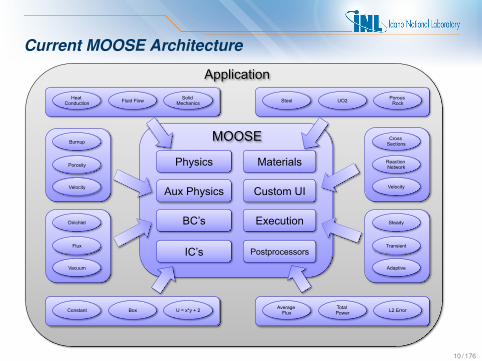
Current MOOSE Architecture
Application
Physics Materials
BC’s
Postprocessors
Custom UI
Execution
Aux Physics
Heat Conduction Fluid Flow Solid
Mechanics
IC’s
Steel UO2 Porous Rock
MOOSE Burnup
Porosity
Velocity
Dirichlet
Flux
Vacuum
Cross Sections
Reaction Network
Velocity
Steady
Transient
Adaptive
Average Flux
Total Power L2 Error Constant Box U = x*y + 2
10 / 176

MOOSE Software Quality Practices
• MOOSE currently meets all NQA-1 (Nuclear Quality Assurance Level 1)requirements
• All commits to MOOSE undergo review using GitHub Pull Requests andmust pass a set of application regression tests before they are available toour users.
• All changes must be accompanied by issue numbers and assigned anappropriate risk level.
• We maintain a regression test code coverage level of 80% or better at alltimes.
• We follow strict code style and formatting guidelines (available on our wiki).
• We monitor code comments with third party tools for better readability.
11 / 176

MOOSE produces results1. M. Tonks, D. Gaston, P. Millett, D. Andrs, and P. Talbot. An object-oriented finite element framework for multiphysics phase field
simulations. Comp. Mat. Sci, 51(1):20–29, 2012.2. R. Williamson, J. Hales, S. Novascone, M. Tonks, D. Gaston, C. Permann, D. Andrs, and R. Martineau. Multidimensional Multiphysics
Simulation of Nuclear Fuel Behavior. Submitted J. Nuclear Materials, 2011.3. M. Tonks, D. Gaston, C. Permann, P. Millett, G. Hansen, C. Newman, and D. Wolf. A coupling methodology for mesoscale-informed
nuclear fuel performance codes. Nucl. Engrg. Design, 240:2877–2883, 2010.4. D. Gaston, G. Hansen, S. Kadioglu, D. Knoll, C. Newman, H. Park, C. Permann, and W. Taitano. Parallel multiphysics algorithms and
software for computational nuclear engineering. Journal of Physics: Conference Series, 180(1):012012, 2009.5. M. Tonks, G. Hansen, D. Gaston, C. Permann, P. Millett, and D. Wolf. Fully-coupled engineering and mesoscale simulations of thermal
conductivity in UO2 fuel using an implicit multiscale approach. Journal of Physics: Conference Series, 180(1):012078, 2009.6. C. Newman, G. Hansen, and D. Gaston. Three dimensional coupled simulation of thermomechanics, heat, and oxygen diffusion in
UO2 nuclear fuel rods. Journal of Nuclear Materials, 392:6–15, 2009.7. D. Gaston, C. Newman, G. Hansen, and D. Lebrun-Grandie. MOOSE: A parallel computational framework for coupled systems of
nonlinear equations. Nucl. Engrg. Design, 239:1768–1778, 2009.8. G. Hansen, C. Newman, D. Gaston, and C. Permann. An implicit solution framework for reactor fuel performance simulation. In 20th
International Conference on Structural Mechanics in Reactor Technology (SMiRT 20), paper 2045, Espoo (Helsinki), Finland, August 9–142009.
9. G. Hansen, R. Martineau, C. Newman, and D. Gaston. Framework for simulation of pellet cladding thermal interaction (PCTI) for fuelperformance calculations. In American Nuclear Society 2009 International Conference on Advances in Mathematics, ComputationalMethods, and Reactor Physics, Saratoga Springs, NY, May 3–7 2009.
10. C. Newman, D. Gaston, and G. Hansen. Computational foundations for reactor fuel performance modeling. In American Nuclear Society2009 International Conference on Advances in Mathematics, Computational Methods, and Reactor Physics, Saratoga Springs, NY, May 3–72009.
11. D. Gaston, C. Newman, and G. Hansen. MOOSE: a parallel computational framework for coupled systems of nonlinear equations. InAmerican Nuclear Society 2009 International Conference on Advances in Mathematics, Computational Methods, and Reactor Physics,Saratoga Springs, NY, May 3–7 2009.
12. L. Guo, H. Huang, D. Gaston, and G. Redden. Modeling of calcite precipitation driven by bacteria-facilitated urea hydrolysis in a flowcolumn using a fully coupled, fully implicit parallel reactive transport simulator. In Eos Transactions American Geophysical Union,90(52), Fall Meeting Supplement, AGU 90(52), San Francisco, CA, Dec 14-18 2009.
13. R. Podgorney, H. Huang, and D. Gaston. Massively parallel fully coupled implicit modeling of coupledthermal-hydrological-mechanical processes for enhanced geothermal system reservoirs. In Proceedings, 35th Stanford GeothermalWorkshop, Stanford University, Palo Alto, CA, Feb 1-3 2010.
14. H. Park, D. Knoll, D. Gaston, and R. Martineau. Tightly Coupled Multiphysics Algorithms for Pebble Bed Reactors. Nuclear Science andEngineering, 166(2):118-133, 2010.
12 / 176

R&D100 Award• In 2014, the MOOSE project received an R&D100 award.
http://www.rdmag.com/award-winners/2014/07/2014-r-d-100-award-winners
• We truly appreciate the outstanding work and dedication of the entireMOOSE development community, this award would not have been possiblewithout it!
13 / 176

C++ FundamentalsOnly what you need to know

Outline• Part 1
– Basic Syntax Review– C++ Definitions, Source Code Organization, Building your Code
• Part 2– Scope– Pointers and References– Dynamic Memory Allocation– Const-ness– Function Overloading
• Part 3– Type System– Brief Intro to Using Templates– C++ Data Structures– Standard Template Library Containers
• Part 4– Object Oriented Design– Classes in C++
15 / 176

Typeface Conventions
• Key concepts
• Special attention required!
• Code
• // Comments
• int x; // Language keywords
16 / 176

MOOSE Coding Standards
• Capitalization– ClassName– methodName– member variable– local variable
• FileNames– src/ClassName.C– include/ClassName.h
• Spacing– Two spaces for each indentation level– Four spaces for initialization lists– Braces should occupy their own line– Spaces around all binary operators and declaration symbols + - * & ...
• No Trailing Whitespace!• Documentation for each method (Doxygen keywords)
– @param– @return– ///Doxygen Style Comment
• See our wiki page for a comprehensive listhttps://hpcsc.inl.gov/moose/wiki/CodeStandards
17 / 176

Part 1• Basic Syntax Review
• C++ Definitions
• Source Code Organization
• Building your Code
18 / 176
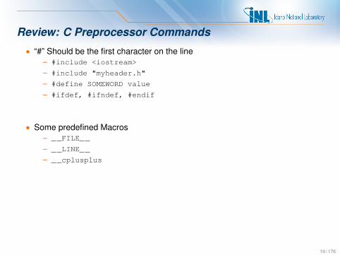
Review: C Preprocessor Commands
• “#” Should be the first character on the line– #include <iostream>
– #include "myheader.h"
– #define SOMEWORD value
– #ifdef, #ifndef, #endif
• Some predefined Macros– FILE
– LINE
– cplusplus
19 / 176
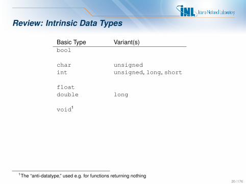
Review: Intrinsic Data Types
Basic Type Variant(s)bool
char unsignedint unsigned, long, short
floatdouble long
void1
1The “anti-datatype,” used e.g. for functions returning nothing20 / 176

Review: Operators
• Math: + - * / % += -= *= /= %= ++ --
• Comparison: < > <= >= != ==
• Logical Comparison: && || !
• Memory: * & new delete sizeof
• Assignment: =
• Member Access:– -> (Access through a pointer)– . (Access through reference or object)
• Name Resolution: ::
21 / 176

Review: Curly Braces
• Used to group statements together
• Creates new layer of scope (we’ll get to this)
22 / 176

Review: Expressions
• Composite mathematical expressions:
a = b * (c - 4) / d++;
• Composite boolean expressions:
if (a && b && f()) e = a;
– Note: Operators && and || use “short-circuiting,” so “b” and “f()” in theexample above may not get evaluated.
• Scope resolution operator:
t = std::pow(r, 2);b = std::sqrt(d);
• Dot and Pointer Operator:
t = my_obj.someFunction();b = my_ptr->someFunction();
23 / 176

Review: Type Casting
float pi = 3.14;
• C-Style:
int approx_pi = (int) pi;
• C++ Styles:
int approx_pi = int(pi);int approx_pi = static cast<int>(pi);
24 / 176

Review: Limits to Type Casting
• Doesn’t work to change to fundamentally different types
float f = (float) "3.14"; // won’t compile
• Be careful with your assumptions
unsigned int huge_value = 4294967295; // okint i = static_cast<int>(huge_value); // won’t work!
25 / 176

Review: Control Statements• For, While, and Do-While Loops:
for (int i=0; i<10; ++i) while (boolean-expression) do while (boolean-expression);
• If-Then-Else Tests:
if (boolean-expression) else if (boolean-expression) else
• In the previous examples, boolean-expression is any valid C++statement which results in true or false. Examples:
– if (0) // Always false
– while (a > 5)
26 / 176

Review: Control Statements
switch (expression)case constant1:// commands to execute if// expression==constant1 ...break;
case constant2:case constant3:// commands to execute if// expression==constant2 OR expression==constant3...break;
default:// commands to execute if no previous case matched
27 / 176

Declarations and Definitions• In C++ we split our code into multiple files
– headers (*.h)– bodies (*.C)
• Headers generally contain declarations– Our statement of the types we will use– Gives names to our types
• Bodies generally contain definitions– Our descriptions of those types, including what they do or how they are built– Memory consumed– The operations functions perform
28 / 176

Declaration Examples
• Free functions:
returnType functionName(type1 name1, type2 name2);
• Object member functions (methods):
class ClassNamereturnType methodName(type1 name1, type2 name2);
;
29 / 176

Definition Examples
• Function definition:
returnType functionName(type1 name1, type2 name2)// statements
• Class method definition:
returnType ClassName::methodName(type1 name1, type2 name2)// statements
30 / 176

Function Example: Addition
#include <iostream>int addition (int a, int b)int r;r=a+b;return r;
int main ()
int z;z = addition (5,3);std::cout << "The result is " << z;return 0;
31 / 176

Addition Cont’d: Separate Definition and Declaration
#include <iostream>int addition (int a, int b);
int main ()
int z = addition (5,3);std::cout << "The result is " << z;return 0;
int addition (int a, int b)return a + b;
32 / 176

Make• A Makefile is a list of dependencies with rules to satisfy those
dependencies
• All MOOSE-based applications are supplied with a complete Makefile
• To build your MOOSE-based application just type:
make
33 / 176

Compiling, Linking, Executing
• Compile and Linkg++ -O3 -o myExample myExample.C
• Compile onlyg++ -O3 -o myExample.o -c myExample.C
• Link onlyg++ -O3 -o myExample myExample.o
34 / 176

Compiler/Linker Flags
• Libraries (-L) and Include (-I) path
• Library Names (-l)– Remove the leading “lib” and trailing file extension when linkinglibutils.so would link as -lutils
g++ -I/home/permcj/include \-L/home/permcj/lib -lutils \-Wall -o myExec myExec.o
35 / 176

Execution• Basic execution./myExec
• Finding shared libraries at runtime– Linux
• ldd• $LD LIBRARY PATH
– Mac• oTool• $DYLD LIBRARY PATH
36 / 176

Recall Addition Example
#include <iostream>int addition (int a, int b); // will be moved to header
int main ()
int z = addition (5,3);std::cout << "The result is " << z;return 0;
int addition (int a, int b)return a + b;
37 / 176

Header File (add.h)
#ifndef ADD_H // include guards#define ADD_H
int addition (int a, int b); // Function declaration
#endif // ADD_H
• Headers typically contain declarations only
38 / 176

Source File (add.C)
#include "add.h"
int addition (int a, int b)return a + b;
39 / 176

Driver Program (main.C)
#include "add.h"#include <iostream>
int main ()
int z = addition(5,3);std::cout << "The result is " << z;return 0;
40 / 176

Compiling the “Addition” Example
1. g++ -g -c -o add.o add.C
2. g++ -g -c -o main.o main.C
3. g++ -g -o main main.o add.o
• The -c flag means compile only, do not link
• These commands can be stored in a Makefile and executed automaticallywith the make command
41 / 176

Part 2• Scope• Pointers and References• Dynamic Memory Allocation• Const-ness• Function Overloading
42 / 176

Scope
• A scope is the extent of the program where a variable can be seen andused.
– local variables have scope from the point of declaration to the end of theenclosing block
– global variables are not enclosed within any scope and are available within theentire file
• Variables have a limited lifetime– When a variable goes out of scope, its destructor is called
• Dynamically-allocated (via new) memory is not automatically freed at theend of scope
43 / 176

“Named” Scopes
• class scope
class MyObjectpublic:
void myMethod();;
• namespace scope
namespace MyNamespacefloat a;void myMethod();
44 / 176

Scope Resolution Operator
• “double colon” :: is used to refer to members inside of a named scope
// definition of the "myMethod" function of "MyObject"void MyObject::myMethod()std::cout << "Hello, World!\n";
MyNamespace::a = 2.718;MyNamespace::myMethod();
• Namespaces permit data organization, but do not have all the featuresneeded for full encapsulation
45 / 176

Assignment (Prequel to Pointers and Refs)
• Recall that assignment in C++ uses the “single equals” operator:
a = b; // Assignment
• Assignments are one of the most common operations in programming
• Two operands are required– An assignable location on the left hand side (memory location)– An expression on the right hand side
46 / 176

Pointers• Pointers are a native type just like an int or long
• Pointers hold the location of another variable or object in memory
47 / 176

Pointer Uses• Pointers are useful in avoiding expensive copies of large objects
– Ex: Functions are passed pointers to large objects, rather than the objectsthemselves
• Pointers also facilitate shared memory– Ex: One object “owns” the memory associated with some data, and allows
others objects access through a pointer
48 / 176

Pointer Syntax
• Declare a pointer
int *p;
• Use the “address-of” operator to initialize a pointer
int a;p = &a;
• Use the “dereference” operator to get or set values pointed-to by the pointer
*p = 5; // set value of "a" through "p"std::cout << *p << "\n"; // prints 5std::cout << a << "\n"; // prints 5
49 / 176

Pointer Syntax, Cont’d
int a = 5;int *p; // declare a pointerp = &a; // set ’p’ equal to address of ’a’*p = *p + 2; // get value pointed to by ’p’, add 2,
// store result in same location
std::cout << a << "\n"; // prints 7std::cout << *p << "\n"; // prints 7std::cout << p << "\n"; // prints an address (0x7fff5fbfe95c)
50 / 176

Pointers Are Powerful But Unsafe• On the previous slide we had this:
p = &a;
• But we can do almost anything we want with p!
p = p + 1000;
• Now what happens when we do this?
*p; // Access memory at &a + 1000
51 / 176

References to the Rescue• A reference is an alternative name for an object [Stroustrup]
– Think of it as an alias for the original variable
int a = 5;int &r = a; // define and initialize a refr = r + 2;
std::cout << a << "\n"; // prints 7std::cout << r << "\n"; // prints 7std::cout << &r << "\n"; // prints address of a
52 / 176

References Are Safe• References cannot be modified
&r = &r + 1; // won’t compile
• References never start out un-initialized
int &r; // won’t compile
• Note that class declarations may contain references
• If so, initialization must occur in the constructor!
• We will see an example later on. . .
53 / 176

Summary: Pointers and References
• A pointer is a variable that holds a memory address to another variable
• A reference is an alternative name for an object [Stroustrup]– Can’t create a reference without an existing object
54 / 176

Summary: Pointers and References
int b = 23int c = 19;
• Pointers
int *iPtr; // DeclarationiPtr = &c;int a = b + *iPtr;
• References
int &iRef = c; // Must initializeint a = b + iRef;
55 / 176

Calling Conventions
• What happens when you make a function call
result = someFunction(a, b, my_shape);
• If the function changes the values inside of a, b or my shape, are thosechanges reflected in my code?
• Is this call expensive? (Are arguments copied around?)
• C++ by default is “Pass by Value” (copy) but you can pass arguments byreference (alias) with additional syntax
56 / 176

Swap Example (Pass by Value)
void swap(int a, int b)int temp = a;a = b;b = temp;
int i = 1;int j = 2;swap (i, j); // i and j are argumentsstd::cout << i << " " << j; // prints 1 2
// i and j are not swapped
57 / 176

Swap Example (Pass by Reference)
void swap(int &a, int &b)int temp = a;a = b;b = temp;
int i = 1;int j = 2;swap (i, j); // i and j are argumentsstd::cout << i << " " << j; // prints 2 1
// i and j are properly swapped
58 / 176

Dynamic Memory Allocation
• Why do we need dynamic memory allocation?– Data size specified at run time (rather than compile time)– Persistence without global variables (scopes)– Efficient use of space– Flexibility
59 / 176

Dynamic Memory in C++
• “new” allocates memory
• “delete” frees memory
• Recall that variables typically have limited lifetimes (within the nearestenclosing scope)
• Dynamic memory allocations do not have limited lifetimes– No automatic memory cleanup!– Watch out for memory leaks– Should have a “delete” for every “new”.
• During normal MOOSE usage, dynamic memory allocation is unnecessary.
60 / 176

Example: Dynamic Memory
int a;int *b;
b = new int; // dynamic allocation, what is b’s value?
a = 4;*b = 5;int c = a + *b;
std::cout << c; // prints 9delete b;
61 / 176

Example: Dynamic Memory Using References
int a;int *b = new int; // dynamic allocationint &r = *b; // creating a reference to newly created variable
a = 4;r = 5;int c = a + r;
std::cout << c; // prints 9delete b;
62 / 176

Const• The const keyword is used to mark a variable, parameter, method or other
argument as constant• Typically used with references and pointers to share objects but guarantee
that they won’t be modified
std::string name("myObject");print(name);...
void print(const std::string & name)// Attempting to modify name here will// cause a compile time error
...
63 / 176

Function Overloading
In C++ you may reuse function names as long as they have different parameterlists or types. A difference only in the return type is not enough to differentiateoverloaded signatures.
int foo(int value);int foo(float value);int foo(float value, bool is_initialized);...
This is very useful when we get to object “constructors”.
64 / 176

Part 3• Type System• Brief Intro to Using Templates• C++ Data Structures• Standard Template Library Containers
65 / 176

Static vs Dynamic Type systems
• C++ is a “statically-typed” language
• This means that “type checking” is performed during compile-time asopposed to run-time
• Python is an example of a “dynamically-typed” language
66 / 176

Static Typing Pros and Cons
• Pros– Safety - compilers can detect many errors– Optimization - compilers can optimize for size and speed– Documentation - The flow of types and their uses in expression is self
documenting
• Cons– More explicit code is needed to convert (“cast”) between types– Abstracting or creating generic algorithms is more difficult
67 / 176

Using Templates
• C++ solves the problem of creating generic containers and algorithms with“templates”
• The details of creating and using templates are extensive, but little basicknowledge is required for simple tasks
template <class T>T getMax (T a, T b)if (a > b)return a;
elsereturn b;
68 / 176

Using Templates
template <class T>T getMax (T a, T b)return (a > b ? a : b); // "ternary" operator
int i = 5, j = 6, k;float x = 3.142; y = 2.718, z;k = getMax(i, j); // uses int versionz = getMax(x, y); // uses float version
k = getMax<int>(i, j); // explicitly calls int version
69 / 176

Compiler Generated Functions
template <class T>T getMax (T a, T b)return (a > b ? a : b);
// generates the following concrete implementationsint getMax (int a, int b)return (a > b ? a : b);
float getMax (float a, float b)return (a > b ? a : b);
70 / 176

Template Specialization
template<class T>void print(T value)std::cout << value << std::endl;
template<>void print<bool>(bool value)if (value)
std::cout << "true";elsestd::cout << "false";
std::cout << std::endl;
int main()int a = 5;bool b = true;
print(a); // prints 5
print(b); // prints true
71 / 176

MOOSE’s validParams Function• The InputParameters class is defined in the header file
“moose/include/utils/InputParameters.h”
• The validParams() function returns an object of typeInputParameters
// template function declaration (InputParameters.h)template<class T>InputParameters validParams();
// Fully-specialized validParams function (YourKernel.h)template<>InputParameters validParams<YourKernel>();
• This function is used by the MOOSE factories and parser for getting, settingand converting parameters from the input file for use inside of your Kernel.
• You need to specialize validParams() for every MooseObject youcreate!
72 / 176

Specialized validParams
#include "MyKernel.h"
template<>InputParameters validParams<MyKernel>()InputParameters params = validParams<Kernel>();params.addParam<Real>("value", 1.0e-5, "Initial Value");params.addCoupledVar("temp", "Coupled Temperature");return params;
73 / 176

C++ Standard Template Library (STL) Data Structures
vectorlistmap multimapset multisetstackqueue priority queuedequebitsetunordered map (next standard “C++11”)unordered set
74 / 176

Using the C++ Vector Container
#include <vector>
int main()
// start with 10 elementsstd::vector<int> v(10);
for (unsigned int i=0; i<v.size(); ++i)v[i] = i;
75 / 176

Using the C++ Vector Container
#include <vector>
int main()
// start with 0 elementsstd::vector<int> v;
for (unsigned int i=0; i<10; ++i)v.push_back(i);
76 / 176

Using the C++ Vector Container
#include <vector>
int main()
// start with 0 elementsstd::vector<int> v;v.resize(10); // creates 10 elements
for (unsigned int i=0; i<10; ++i)v[i] = i;
77 / 176

More features• Containers can be nested to create more versatile structures
std::vector<std::vector<Real> > v;
• To access the items:
for (unsigned int i=0; i < v.size(); ++i)for (unsigned int j=0; j < v[i].size(); ++j)std::cout << v[i][j];
78 / 176

Part 4• Object Oriented Design
– Data Encapsulation– Inheritance– Polymorphism
• Classes in C++– Syntax– Constructors, Destructors
79 / 176
Object-Oriented Definitions
• A “class” is a new data type.
• Contains data and methods for operating on that data– You can think of it as a “blue print” for building an object.
• An “interface” is defined as a class’s publicly available “methods” and “data”
• An “instance” is a variable of one of these new data types.– Also known as an “object”– Analogy: You can use one “blue-print” to build many buildings. You can use one
“class” to build many “objects”.
80 / 176

Object Oriented Design
• Instead of manipulating data, one manipulates objects that have definedinterfaces
• Data encapsulation is the idea that objects or new types should be blackboxes. Implementation details are unimportant as long as an object worksas advertised without side effects.
• Inheritance gives us the ability to abstract or “factor out” common data andfunctions out of related types into a single location for consistency (avoidscode duplication) and enables code re-use.
• Polymorphism gives us the ability to write generic algorithms thatautomatically work with derived types.
81 / 176

Encapsulation (Point.h)
class Pointpublic:
// ConstructorPoint(float x, float y);
// Accessorsfloat getX();float getY();void setX(float x);void setY(float y);
private:float _x, _y;
;
82 / 176

Constructors• The method that is called explicitly or implicitly to build an object• Always has the same name as the class with no return type• May have many overloaded versions with different parameters• The constructor body uses a special syntax for initialization called an
initialization list• Every member that can be initialized in the initialized list - should be
– References have to be initialized here
Point::Point(float x, float y):// Point has no base class, if it did, it// would need to be constructed firstx(x),y(y)
// The body is often empty
83 / 176

Point Class Definitions (Point.C)
#include "Point.h"
Point::Point(float x, float y): x(x), y(y)
float Point::getX() return _x; float Point::getY() return _y; void Point::setX(float x) _x = x; void Point::setY(float y) _y = y;
• The data is safely encapsulated so we can change the implementationwithout affecting users of this type
84 / 176

Changing the Implementation (Point.h)
class Pointpublic:Point(float x, float y);float getX();float getY();void setX(float x);void setY(float y);
private:// Store a vector of values rather than separate scalarsstd::vector<float> coords;
;
85 / 176

New Point Class Body (Point.C)
#include "Point.h"
Point::Point(float x, float y)
coords.push back(x);coords.push back(y);
float Point::getX() return coords[0]; float Point::getY() return coords[1]; void Point::setX(float x) coords[0] = x; void Point::setY(float y) coords[1] = y;
86 / 176

Using the Point Class (main.C)
#include "Point.h"
int main()
Point p1(1, 2);Point p2 = Point(3, 4);Point p3; // compile error, no default constructor
std::cout << p1.getX() << "," << p1.getY() << "\n"<< p2.getX() << "," << p2.getY() << "\n";
87 / 176

Outline Update
• Object Oriented Design– Data Encapsulation– Inheritance– Polymorphism
• Classes in C++– Syntax– Constructors, Destructors
88 / 176

A More Advanced Example (Shape.h)
class Shape public:
Shape(int x=0, int y=0): _x(x), _y(y) // Constructorvirtual ∼Shape() // Destructorvirtual float area()=0; // Pure Virtual Functionvoid printPosition(); // Body appears elsewhere
protected:// Coordinates at the centroid of the shapeint _x;int _y;
;
89 / 176

The Derived Classes (Rectangle.h)
#include "Shape.h"
class Rectangle: public Shapepublic:
Rectangle(int width, int height, int x=0, int y=0):Shape(x,y),_width(width),_height(height)
virtual ∼Rectangle() virtual float area() return _width * _height;
protected:int _width;int _height;
;
90 / 176

The Derived Classes (Circle.h)
#include "Shape.h"
class Circle: public Shapepublic:
Circle(int radius, int x=0, int y=0):Shape(x,y), _radius(radius)
virtual ∼Circle() virtual float area() return PI * _radius * _radius;
protected:int _radius;
;
91 / 176

Is-A• When using inheritance, the derived class can be described in terms of the
base class– A Rectangle “is-a” Shape
• Derived classes are “type” compatible with the base class (or any of itsancestors)
– We can use a base class variable to point to or refer to an instance of a derivedclass
Rectangle rectangle(3, 4);Shape & s_ref = rectangle;Shape * s_ptr = &rectangle;
92 / 176

Writing a generic algorithm
// create a couple of shapesRectangle r(3, 4);Circle c(3, 10, 10);
printInformation(r); // pass a Rectangle into a Shape referenceprintInformation(c); // pass a Circle into a Shape reference
...
void printInformation(const Shape & shape)shape.printPosition();std::cout << shape.area() << ’\n’;
// (0, 0)// 12// (10, 10)// 28.274
93 / 176

Homework Ideas
1. Implement a new Shape called Square. Try deriving from Rectangledirectly instead of Shape. What advantages/disadvantages do the twodesigns have?
2. Implement a Triangle shape. What interesting subclasses of Trianglecan you imagine?
3. Add another constructor to the Rectangle class that accepts coordinatesinstead of height and width.
94 / 176

Deciphering Long Declarations
• Read the declaration from right to left
Mesh *mesh;
– mesh is a pointer to a Mesh object
InputParameters ¶ms;
– params is a reference to an InputParameters object
95 / 176

Finite ElementsThe MOOSE way

Polynomial Fitting
• To introduce the idea of finding coefficients to functions, let’s considersimple polynomial fitting.
• In polynomial fitting (or interpolation) you have a set of points and you arelooking for the coefficients to a function that has the form:
f (x) = a + bx + cx2 + . . .
• Where a, b and c are scalar coefficients and 1, x , x2 are “basis functions”.• The idea is to find a, b, c, etc. such that f (x) passes through the points you
are given.• More generally you are looking for:
f (x) =d∑
i=0
cix i
• where the ci are coefficients to be determined.• f (x) is unique and interpolary if d + 1 is the same as the number of points
you need to fit.• Need to solve a linear system to find the coefficients.
97 / 176

Example
Pointsx y1 43 14 2
Linear System1 1 11 3 91 4 16
abc
=
412
Solution 8
− 29656
f (x) = 8− 296
x +56
x2
98 / 176
Example Continued
• First, note that the coefficients themselves don’t mean anything.– By themselves they are just numbers.
• Second, the solution is not the coefficients, but rather the function theycreate when they are multiplied by their respective basis functions andsummed.
• Yes, f (x) does go through the points we were given, but it is also definedeverywhere in between.
• We can evaluate f (x) at the point x = 2 (say) by computing:
f (2) =2∑
i=0
ci2i , or more generically: f (2) =2∑
i=0
cigi(2)
where the ci correspond to the coefficients in the solution vector, and the gi
are the respective functions.• Finally: Note that the matrix consists of evaluating the functions at the
points.
99 / 176

Finite Elements Simplified
• A method for numerically approximating the solution to Partial DifferentialEquations (PDEs).
• Works by finding a solution function that is made up of “shape functions”multiplied by coefficients and added together.
– Just like in polynomial fitting, except the functions aren’t typically as simple asx i (although they can be!).
• The Galerkin Finite Element method is different from finite difference andfinite volume methods because it finds a piecewise continuous functionwhich is an approximate solution to the governing PDE.
– Just as in polynomial fitting you can evaluate a finite element solution anywherein the domain.
– You do it the same way: by adding up “shape functions” evaluated at the pointand multiplied by their coefficient.
• FEM is widely applicable for a large range of PDEs and domains.• It is supported by a rich mathematical theory with proofs about accuracy,
stability, convergence and solution uniqueness.
100 / 176

Weak Form• Using FE to find the solution to a PDE starts with forming a “weighted
residual” or “variational statement” or “weak form”.– We typically refer to this process as generating a Weak Form.
• The idea behind generating a weak form is to give us some flexibility, bothmathematically and numerically.
• A weak form is what you need to input into MOOSE in order to solve a newproblem.
• Generating a weak form generally involves these steps:1. Write down strong form of PDE.2. Rearrange terms so that zero is on the right of the equals sign.3. Multiply the whole equation by a “test” function (ψ).4. Integrate the whole equation over the domain (Ω).5. Integrate by parts (use the divergence theorem) to get the desired derivative
order on your functions and simultaneously generate boundary integrals.6. Code up with MOOSE . . . and run!
101 / 176

Refresher: The divergence theorem
• Transforms a volume integral into a surface integral:∫Ω
∇ · F dx =
∫∂Ω
F · n ds
• In finite element calculations, for example with F = −k(x)∇u, thedivergence theorem implies:
−∫
Ω
ψ (∇ · k(x)∇u) dx =
∫Ω
∇ψ · k(x)∇u dx −∫∂Ω
ψ (k(x)∇u · n) ds
• In this talk, we will use the following inner product notation to representintegrals since it is more compact:
− (ψ,∇ · k(x)∇u) = (∇ψ, k(x)∇u)− 〈ψ, k(x)∇u · n〉
• http://en.wikipedia.org/wiki/Divergence_theorem
102 / 176

Example: Convection Diffusion
1. −∇ · k∇u + β · ∇u = f
2. −∇ · k∇u + β · ∇u − f = 0
3. −ψ (∇ · k∇u) + ψ (β · ∇u)− ψf = 0
4. −∫
Ω
ψ (∇ · k∇u) +∫
Ω
ψ (β · ∇u)−∫
Ω
ψf = 0
5.∫
Ω
∇ψ · k∇u −∫∂Ω
ψ (k∇u · n) +∫
Ω
ψ (β · ∇u)−∫
Ω
ψf = 0
6. (∇ψ, k∇u)︸ ︷︷ ︸Kernel
−〈ψ, k∇u · n〉︸ ︷︷ ︸BC
+(ψ,β · ∇u)︸ ︷︷ ︸Kernel
− (ψ, f )︸ ︷︷ ︸Kernel
= 0
103 / 176

More Depth
• While the weak form is essentially what you need for adding physics toMOOSE, in traditional finite element software more work is necessary.
• The next step is to discretize the weak form by selecting an expansion of u:
u ≈ uh =N∑
j=1
ujφj
– The φj are generally called “shape functions”– In the expansion of uh, the φj are sometimes called “trial functions”– Analogous to the xn we used earlier
• The gradient of u can be expanded similarly:
∇u ≈ ∇uh =N∑
j=1
uj∇φj
• In the Galerkin finite element method, the same shape functions are usedfor both the trial and test functions
ψ = φiNi=1
104 / 176

More Depth
• Substituting these expansions back into our weak form, we get:
(∇ψi , k∇uh)− 〈ψi , k∇uh · n〉+ (ψi ,β · ∇uh)− (ψi , f ) = 0, i = 1, . . . ,N
• The left-hand side of the equation above is what we generally refer to asthe i th component of our “Residual Vector” and write as Ri(uh).
105 / 176

Shape Functions
• Shape Functions are the functions that get multiplied by coefficients andsummed to form the solution.
• They are analogous to the xn functions from polynomial fitting (in fact, youcan use those as shape functions!).
• Typical shape function families: Lagrange, Hermite, Hierarchic, Monomial,Clough-Toucher
– MOOSE has support for all of these.
• Lagrange shape functions are the most common.– They are interpolary at the nodes.– This means the coefficients correspond to the values of the functions at the
nodes.
106 / 176

Some 1D Shape Functions
0
0.2
0.4
0.6
0.8
1
-1 -0.5 0 0.5 1
ξ
Linear Lagrange Shape Functions
ψ0 ψ1
-0.2
0
0.2
0.4
0.6
0.8
1
-1 -0.5 0 0.5 1
ξ
Quadratic Lagrange Shape Functions
ψ0 ψ1
ψ2
-0.5
0
0.5
1
1.5
-1 -0.5 0 0.5 1
ξ
Cubic Lagrange Shape Functions
ψ0 ψ1
ψ2 ψ3
-0.4
-0.2
0
0.2
0.4
0.6
0.8
1
-1 -0.5 0 0.5 1
ξ
Cubic Hermite Shape Functions
ψ0
ψ1
ψ2
ψ3
107 / 176

2D Lagrange Shape Functions
• Some biquadratic basis functions defined on the Quad9 element:
ψ0 ψ4 ψ8
• ψ0 is associated to a “corner” node, it is zero on the opposite edges.• ψ4 is associated to a “mid-edge” node, it is zero on all other edges.• ψ8 is associated to the “center” node, it is symmetric and ≥ 0 on the
element.
108 / 176

Numerical Integration
• The only analytical piece left in the weak form is the integrals.
• To compute these integrals numerically, we use quadrature (typically “GaussianQuadrature”).
• Quadrature approximates continuous integrals by discrete sums:∫f (x) ≈
∑qp
f (xqp)wqp (1)
– Here xqp is the position of the quadrature point, and wqp is the associated weight.
• Under certain common situations, the approximation (1) is exact!– Ex: In 1 dimension, Gaussian Quadrature can exactly integrate polynomials of order
2n − 1 with n quadrature points.
109 / 176

Numerical Integration
• Note that sampling u for quadrature amounts to:
u(xqp) ≈ uh(xqp) =∑
ujφj(xqp)
∇u(xqp) ≈ ∇uh(xqp) =∑
uj∇φj(xqp)
• And our weak form becomes:
Ri(uh) =∑qp
wqp∇ψi(xqp) · k(xqp)∇uh(xqp)
−∑qpface
wqpfaceψi(xqpface )k(xqpface )∇uh(xqpface ) · n(xqpface )
+∑qp
wqpψi(xqp) (β(xqp) · ∇uh(xqp))
−∑qp
wqpψi(xqp)f (xqp)
110 / 176

Newton’s Method• We now have a nonlinear system of equations,
Ri(uh) = 0, i = 1, . . . ,N
to solve for the coefficients uj , j = 1, . . . ,N.
• Newton’s method has good convergence properties, we use it to solve thissystem of nonlinear equations.
• Newton’s method is a “root finding” method: it finds zeros of nonlinearequations.
• Newton’s Method in “Update Form” for f (x) : R→ R
f ′(xn)δxn+1 = −f (xn)
xn+1 = xn + δxn+1
111 / 176

Newton’s Method Continued• We don’t have just one scalar equation: we have a system of nonlinear
equations.• This leads to the following form of Newton’s Method:
J(un)δun+1 = −R(un)
un+1 = un + δun+1
• Where J(un) is the Jacobian matrix evaluated at the current iterate:
Jij(un) =∂Ri(un)
∂uj
• Note that:
∂uh
∂uj=∑
k
∂
∂uj(ukφk ) = φj
∂ (∇uh)
∂uj=∑
k
∂
∂uj(uk∇φk ) = ∇φj
112 / 176

Newton For A Simple Equation
• Consider the convection-diffusion equation with nonlinear k , β and f :
−∇ · k∇u + β · ∇u = f
• The i th component of the residual vector is:
Ri(uh) = (∇ψi , k∇uh)− 〈ψi , k∇uh · n〉+ (ψi ,β · ∇uh)− (ψi , f )
• Using the previously defined rules for ∂uh∂uj
and ∂(∇uh)∂uj
the (i , j) entry of theJacobian is then:
Jij(uh) =
(∇ψi ,
∂k∂uj∇uh
)+ (∇ψi , k∇φj)−
⟨ψi ,
∂k∂uj∇uh · n
⟩− 〈ψi , k∇φj · n〉
+
(ψi ,
∂β
∂uj· ∇uh
)+ (ψi ,β · ∇φj)−
(ψi ,
∂f∂uj
)• Note that even for this “simple” equation the Jacobian entries are nontrivial,
especially when the partial derivatives of k , β and f are actually expanded.• In a multiphysics setting with many coupled equations and complicated
material properties, the Jacobian might be extremely difficult to determine.
113 / 176

Chain Rule• On the previous slide, the term ∂f
∂ujwas used, where f was a nonlinear
forcing function.• The chain rule allows us to write this term as
∂f∂uj
=∂f∂uh
∂uh
∂uj
=∂f∂uh
φj
• If a functional form of f is known, e.g. f (u) = sin(u), this formula impliesthat its Jacobian contribution is given by
∂f∂uj
= cos(uh)φj
114 / 176

Jacobian Free Newton Krylov
• J(un)δun+1 = −R(un) is a linear system of equations to solve during eachNewton step.
• We typically employ GMRES (a Krylov method) for this:– Scales well in parallel.– Effective on a diverse set of problems.
• In a Krylov method (such as GMRES) we have the representation:
δun+1,k = a0r0 + a1Jr0 + a2J2r0 + · · ·+ ak Jk r0
• Note that J is never explicitly needed. Instead, only the action of J on avector needs to be computed.
• This action can be approximated by:
Jv ≈ R(u + εv)− R(u)ε
• This form has many advantages:– No need to do analytic derivatives to form J– No time needed to compute J (just residual computations)– No space needed to store J
115 / 176

Wrap Up
• The Finite Element Method is a way of numerically approximating thesolution to PDEs.
• Just like polynomial fitting, FEM finds coefficients for basis functions.
• The “solution” is the combination of the coefficients and the basis functions,and the solution can be sampled anywhere in the domain.
• We compute integrals numerically using quadrature.
• Newton’s Method provides a mechanism for solving a system of nonlinearequations.
• The Jacobian Free Newton Krylov (JFNK) method allows us to circumventtedious (and error prone) derivative calculations.
116 / 176

The MOOSE Framework

MOOSE Requirements
• MOOSE requires several pieces of software to be in place before it willbuild:
– MPI– Hypre (Optionally if you want to use AMG)– PETSc– libMesh
• If you are working on your own workstation you will have to compile / installall of these.
• We maintain binary builds of these packages for the following operatingsystems:
– Ubuntu (deb), OpenSUSE (rpm), tarball installer coming soon– OS X 10.7, 10.8, and 10.9
• https://www.mooseframework.org
– Getting Started Instructions– Issue System– Documentation, Blog, and Wiki
118 / 176

Anatomy
• Any MOOSE-based application should have the following directorystructure:application/
LICENSEMakefilerun_testsdoc/lib/src/
main.Cbase/actions/auxkernels/bcs/dampers/dirackernels/executioners/functions/ics/kernels/materials/postprocessors/utils/
tests/... (same stuff as src)
119 / 176

Looking at MOOSE
• All classes are separated out into directories associated with that set ofclasses:
– kernels/– bcs/– ics/– auxkernels/– dgkernels/– functions/– actions/– etc. . .
120 / 176

The Input File

The Input File
• By default MOOSE uses a hierarchical, block-structured input file.
• Within each block, any number of name/value pairs can be listed.
• The syntax is completely customizable, or replaceable.
• To specify a simple problem, you will need to populate five or six top-levelblocks.
• We will briefly cover a few of these blocks in this section and will illustratethe usage of the remaining blocks throughout this manual.
122 / 176

Main Input File Blocks
• MOOSE expects the following basic blocks for a simple problem:– [Mesh]
– [Variables]
– [Kernels]
– [BCs]
– [Executioner]
– [Outputs]
123 / 176

Hierarchical Block-Structure
[Variables]active = ’u’
[./u]order = FIRSTfamily = LAGRANGE
[../]
[./v]order = FIRSTfamily = LAGRANGE
[../][]
[Kernels]...
[]
• The u and v blocks define variables, sincethey are declared in the Variables block.
• The active line can be used to turn on/offvariables quickly. In this case, only the uvariable will be used in the simulation. Anabsent active line means all variablesare active.
• The block names are user-defined, butmust be unique and should not containnon-ASCII characters.
124 / 176

The Mesh Block
[Mesh]# Optional Typetype = <FileMesh | GeneratedMesh>
# FileMeshfile = <filename>
# Some other commonly used optionsuniform_refine = <n>second_order = <true|false>
[]
• The Mesh block is generally associatedwith an Action that reads and/orconstructs the mesh for the simulation.
• The default type, FileMesh, issuitable for reading any normal meshformat from a file.
• The base class MooseMesh can beextended to construct or modify yourown Meshes during runtime asneeded.
• There are additional advanced optionsfor this and the following blocks whichare not listed in this section. . .
125 / 176

The Variables Block
[Variables][./nonlinear_variable1]
order = <FIRST | SECOND | ...>family = <LAGRANGE | HERMITE | ...>
[../]
[./nonlinear_variable2]...
[../][]
• The Variables block declares thenonlinear variables that will be solvedfor in the simulation.
• The default order and family are FIRSTand LAGRANGE, respectively.
126 / 176

The Kernels Block
[Kernels][./my_kernel1]
type = <Any Registered Kernel>variable = <Nonlinear Variable Name>
[../]
[./my_kernel2]...
[../][]
• The Kernels block declares PDEoperators that will be used in thesimulation.
• The type parameter is used to specifythe type of kernel to instantiate.
127 / 176
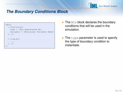
The Boundary Conditions Block
[BCs][./bottom_bc]
type = <Any Registered BC>variable = <Nonlinear Variable Name>
[../]
[./top_bc]...
[../][]
• The BCs block declares the boundaryconditions that will be used in thesimulation.
• The type parameter is used to specifythe type of boundary condition toinstantiate.
128 / 176

The Executioner Block
[Executioner]type = <Steady | Transient | ...>
[]
• The Executioner block declares theexecutioner that will be used in thesimulation.
• The type parameter is used to specifythe type of executioner to instantiate.
129 / 176

The Outputs Block
[Outputs]file_base = <base_file_name>exodus = trueconsole = true
[]
• The Outputs block controls thevarious output (to screen and file) usedin the simulation.
130 / 176

Example Input File
[Mesh]file = mug.e
[]
[Variables]active = ’diffused’
[./diffused]order = FIRSTfamily = LAGRANGE
[../][]
[Kernels]active = ’diff’
[./diff]type = Diffusionvariable = diffused
[../][]
[BCs]active = ’bottom top’
[./bottom]type = DirichletBCvariable = diffusedboundary = ’bottom’value = 1
[../]
[./top]type = DirichletBCvariable = diffusedboundary = ’top’value = 0
[../][]
[Executioner]type = Steady
[]
[Outputs]file_base = outexodus = trueconsole = true
[]
131 / 176

Look at Example 1 (page E3)
132 / 176
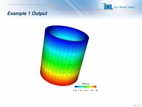
Example 1 Output
133 / 176
The Mesh Block and Types

Creating a Mesh
• For complicated geometries, we generally use CUBIT from Sandia NationalLaboratories.
• CUBIT can be licensed from CSimSoft for a fee depending on the type oforganization you work for.
• Other mesh generators can work as long as they output a file format thatlibMesh reads (next slide).
• If you have a specific mesh format that you like, we can take a look atadding support for it to libMesh.
135 / 176

CUBIT Interface
136 / 176
Boundary ConditionList
GeometryList
CommandLine Interface
ToolsInterface

FileMesh• FileMesh is the default type when the “type” parameter is omitted from theMesh section.
• MOOSE supports reading and writing a large number of formats and couldbe extended to read more.
.dat Tecplot ASCII file
.e, .exd Sandia’s ExodusII format
.fro ACDL’s surface triangulation file
.gmv LANL’s GMV (General Mesh Viewer) format
.mat Matlab triangular ASCII file (read only)
.msh GMSH ASCII file (write only)
.n, .nem Sandia’s Nemesis format
.plt Tecplot binary file (write only)
.poly TetGen ASCII file (write only)
.inp Abaqus .inp format (read only)
.ucd AVS’s ASCII UCD format
.unv I-deas Universal format
.xda, .xdr libMesh formats
.vtk Visualization Toolkit
137 / 176
Generated Mesh• type = GeneratedMesh
• Built-in mesh generation is implemented for lines, rectangles, andrectangular prisms (“boxes”) but could be extended.
• The sides of a GeneratedMesh are named in a logical way (bottom, top,left, right, front, and back).
• The length, width, and height of the domain, and the number of elements ineach direction can be specified independently.
138 / 176

Named Entity Support
...[Mesh]
file = three_block.e
# These names will be applied on the# fly to the mesh so that they can be# used in the input file. In addition# they will be written to the output# fileblock id = ’1 2 3’block name = ’wood steel copper’
boundary id = ’1 2’boundary name = ’left right’
[]...
• Human-readable names can beassigned to blocks, sidesets, andnodesets. These names will beautomatically read in and can be usedthroughout the input file.
• This is typically done inside of Cubit.• Any parameter that takes entity IDs in
the input file will accept either numbersor “names”.
• Names can also be assigned to IDson-the-fly in existing meshes to easeinput file maintenance (see example).
• On-the-fly names will also be written toExodus/XDA/XDR files.
139 / 176

Parallel Mesh• Useful when the mesh data structure dominates memory usage.
• Only the pieces of the mesh “owned” by processor N are actually stored byprocessor N.
• If the mesh is too large to read in on a single processor, it can be split priorto the simulation.
– Copy the mesh to a large memory machine.
– Use a tool to split the mesh into n pieces (SEACAS, loadbal).
– Copy the pieces to your working directory on the cluster.
– Use the Nemesis reader to read the mesh using n processors.
• See nemesis test.i in the moose test directory for a workingexample.
140 / 176

Displaced Mesh
• Calculations can take place in either the initial mesh configuration or, whenrequested, the “displaced” configuration.
• To enable displacements, provide a vector of displacement variable namesfor each spatial dimension in the Mesh section, e.g.:
displacements = ’disp_x disp_y disp_z’
• Once enabled, the parameter use displaced mesh can be set onindividual MooseObjects which will enable them to use displacedcoordinates during calculations:
template<>InputParameters validParams<SomeKernel>()
InputParameters params = validParams<Kernel>();params.set<bool>("use_displaced_mesh") = true;return params;
• This can also be set in the input file, but it’s a good idea to do it in code ifyou have a pure Lagrangian formulation.
141 / 176
Mesh Modifiers• [MeshModifiers] further modify the mesh after it has been created.
• Possible modifications include: adding node sets, translating, rotating, andscaling the mesh points.
• Users can create their own MeshModifiers by inheriting fromMeshModifier and defining a custom modify() function.
• A few built-ins:– AddExtraNodeset– SideSetFromNormals, SideSetFromPoints– Transform – Scale, Rotate, Translate– MeshExtruder
142 / 176
Extrusion
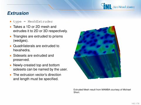
• type = MeshExtruder
• Takes a 1D or 2D mesh andextrudes it to 2D or 3D respectively.
• Triangles are extruded to prisms(wedges).
• Quadrilaterals are extruded tohexahedra.
• Sidesets are extruded andpreserved.
• Newly-created top and bottomsidesets can be named by the user.
• The extrusion vector’s directionand length must be specified.
Extruded Mesh result from MAMBA courtesy of MichaelShort.
143 / 176

The Outputs Block
The Outputs Block
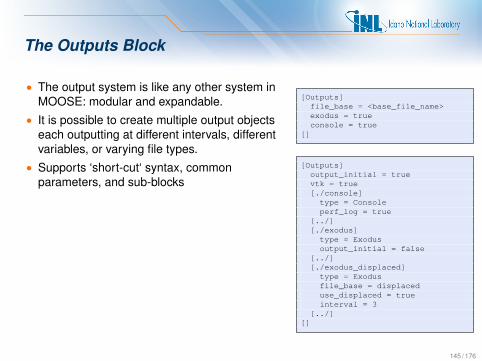
• The output system is like any other system inMOOSE: modular and expandable.
• It is possible to create multiple output objectseach outputting at different intervals, differentvariables, or varying file types.
• Supports ‘short-cut‘ syntax, commonparameters, and sub-blocks
[Outputs]file_base = <base_file_name>exodus = trueconsole = true
[]
[Outputs]output_initial = truevtk = true[./console]
type = Consoleperf_log = true
[../][./exodus]
type = Exodusoutput_initial = false
[../][./exodus_displaced]
type = Exodusfile_base = displaceduse_displaced = trueinterval = 3
[../][]
145 / 176

Supported Formats
Format Short-cut Syntax Sub-block Type
Console (screen) console = true type = ConsoleExodus II exodus = true type = ExodusVTK vtk = true type = VTKGMV gmv = true type = GMVNemesis nemesis = true type = NemesisTecplot tecplot = true type = TecplotXDA xda = true type = XDAXDR xdr = true type = XDRCSV csv = true type = CSVGnuplot gnuplot = true type = GnuplotCheckpoint checkpoint = true type = Checkpoint
146 / 176

Over Sampling
• None of the generally available visualizationpackages currently display higher-ordersolutions (quadratic, cubic, etc.) natively.
• To work around this limitation, MOOSE can“oversample” a higher-order solution byprojecting it onto a finer mesh of linearelements.
• Note: This is not mesh adaptivity, nor does itimprove the solution’s accuracy in general.
• The following slide shows a sequence ofsolutions oversampled from a base solution onsecond-order Lagrange elements.
[Outputs]console = true[./exodus]
file_base = out_oversampletype = Exodusoversample = truerefinements = 3
[../][]
147 / 176

Over Sampling Refinements: 0 to 5 levels
148 / 176
Over Sampling (Cont.)
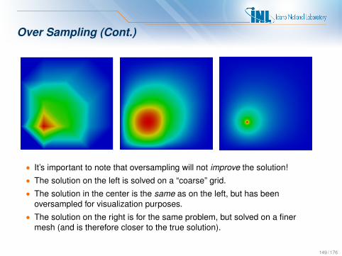
• It’s important to note that oversampling will not improve the solution!• The solution on the left is solved on a “coarse” grid.• The solution in the center is the same as on the left, but has been
oversampled for visualization purposes.• The solution on the right is for the same problem, but solved on a finer
mesh (and is therefore closer to the true solution).
149 / 176
Input Parameters and MOOSETypes

Valid Parameters• A set of custom parameters (InputParameters) is used to construct
every MOOSE object.
• Every MOOSE-derived object must specify a validParams function.
• In this function you must start with the parameters from your parent class(like Kernel) and then specify additional parameters.
• This function must return a set of parameters that the corresponding objectrequires in order to be constructed.
• This design allows users to control any and all parameters they need forconstructing objects while leaving all C++ constructors uniform andunchanged.
151 / 176

Defining Valid Parameters
In the .h file:
class Convection;
template<>InputParameters validParams<Convection>();
class Convection : public Kernel...
In the .C file:
template<>InputParameters validParams<Convection>()
InputParameters params = validParams<Kernel>(); // Must get from parentparams.addRequiredParam<RealVectorValue>("velocity", "Velocity Vector");params.addParam<Real>("coefficient", "Diffusion coefficient");return params;
152 / 176

On the Fly Documentation
• The parser object is capable of generating documentation from thevalidParams functions for each class that specializes that function.
• Option 1: Mouse-over when using the MOOSE GUI “peacock”
• Option 2: Generate a complete tree of registered objects– CLI option --dump [optional search string]– The search string may contain wildcard characters– Searches both block names and parameters– All parameters are printed for a matching block
• Option 3: Generate a tree based on your input file– CLI option --show-input
• Option 4: View it online– http://mooseframework.org/wiki/InputFileSyntax
153 / 176

The InputParameters Object
• The parser and Peacock work with the InputParameters object to readalmost any kind of parameter.
• Built-in types and std::vector are supported via templated methods:– addRequiredParam<Real>("required const", "doc");– addParam<int>("count", 1, "doc"); // default supplied– addParam<unsigned int>("another num", "doc");– addRequiredParam<std::vector<int> >("vec", "doc");
• Other supported parameter types include:– Point– RealVectorValue– RealTensorValue– SubdomainID– BoundaryID
• For the complete list of supported types seeParser::extractParams(...)
154 / 176

The InputParameters Object (cont.)
• MOOSE uses a large number of string types to make Peacock morecontext-aware. All of these types can be treated just like strings, but willcause compile errors if mixed improperly in the template functions.
SubdomainNameBoundaryNameFileName MeshFileName OutFileNameVariableName NonlinearVariableName AuxVariableNameFunctionNameUserObjectNamePostprocessorNameIndicatorNameMarkerName
• For a complete list, see the instantiations at the bottom of MooseTypes.h
155 / 176

Default and Range-checked Parameters
• You may supply a default value for all optional parameters (not required)
addParam<RealVectorValue>("direction", RealVectorValue(0,1,0), "doc");
• The following types allow you to supply scalar defaults in place of object:– Any coupled variable– Postprocessors (PostprocessorName)– Functions (FunctionName)
• You may supply an expression to perform range checking within theparameter system.
• You should use the name of your parameter in the expression.
addRangeCheckedParam<Real>("temp", "temp>=300 & temp<=330", "doc");
• Function Parser Syntaxhttp://warp.povusers.org/FunctionParser/fparser.html
156 / 176

MooseEnum• MOOSE includes a “smart” enum utility to overcome many of the
deficiencies in the standard C++ enum type.
• It works in both integer and string contexts and is self-checked forconsistency.
#include "MooseEnum.h"...// The valid options are specified in a space separated list.// You can optionally supply the default value as a second argument.// MooseEnums are case preserving but case-insensitive.MooseEnum option_enum("first=1 second fourth=4", "second");
// Use in a string contextif (option_enum == "first")
doSomething();
// Use in an integer contextswitch(option_enum)case 1: ... break;case 2: ... break;case 4: ... break;default: ... ;
157 / 176

Using MooseEnum with InputParameters
• Objects that have a specific set of named options should use a MooseEnumso that parsing and error checking code can be omitted.
template<>InputParameters validParams<MyObject>()
InputParameters params = validParams<ParentObject>();
MooseEnum component("X Y Z"); // No default suppliedparams.addRequiredParam<MooseEnum>("component", component,
"The X, Y, or Z component");return params;
...
// Assume we’ve saved off our MooseEnum into a instance variable: _componentReal value = 0.0;if (_component.isValid())
value = _some_vector[ component];
• The Peacock GUI will create a drop box when using MooseEnum.
• If the user supplies an invalid option, the parser will catch it and throw aninformative error message.
158 / 176

Multi-value MooseEnums (MultiMooseEnum)
• Works the same way as MooseEnum but supports multiple orderedoptions.
template<>InputParameters validParams<MyObject>()
InputParameters params = validParams<ParentObject>();
MultiMooseEnum transforms("scale rotate translate");params.addRequiredParam<MultiMooseEnum>("transforms", transforms,
"The transforms to perform");return params;
...
if (_transforms.isValid())for (unsigned int i=0; i<_transforms.size(); ++i)
performTransform( transforms[i]);
• Can also ask if item is stored in the MultiMooseEnum by callingtransforms.contains(item);
159 / 176

MultiAppsAdvanced Topic

MultiApps
• MOOSE was originally created to solve fully-coupled systems of PDEs.
• Not all systems need to be / are fully coupled:– Multiscale systems are generally loosely coupled between scales.– Systems with both fast and slow physics can be decoupled in time.– Simulations involving input from external codes might be solved somewhat
decoupled.
• To MOOSE these situations look like loosely-coupled systems offully-coupled equations.
• A MultiApp allows you to simultaneously solve for individual physicssystems.
161 / 176

MultiApps (Cont.)
Master
Mul*App 1 Mul*App 2
Sub-‐app 1-‐1
Sub-‐app 1-‐2
Sub-‐app 2-‐1
Sub-‐app 2-‐2
Mul*App 3 Mul*App 4
Sub-‐app 3-‐1
Sub-‐app 3-‐2
Sub-‐app 4-‐1
Sub-‐app 4-‐2
Sub-‐app 2-‐3
• Each “App” is considered to be a solve thatis independent.
• There is always a “master” App that isdoing the “main” solve.
• A “master” App can then have any numberof MultiApps.
• Each MultiApp can represent many(hence Multi!) “sub-apps”.
• The sub-apps can be solving for completelydifferent physics from the main application.
• They can be other MOOSE applications, ormight represent external applications.
• A sub-app can, itself, have MultiApps...leading to multi-level solves.
162 / 176

Input File Syntax
[MultiApps][./some_multi]
type = TransientMultiAppapp_type = SomeAppexecute_on = timesteppositions = ’0.0 0.0 0.0
0.5 0.5 0.00.6 0.6 0.00.7 0.7 0.0’
input_files = ’sub.i’[../]
[]
• MultiApps are declared in the MultiAppsblock.
• They require a type just like any other block.• app type is required and is the name of theMooseApp derived App that is going to be run.Generally this is something like AnimalApp.
• A MultiApp can be executed at any pointduring the master solve. You set that usingexecute on to one of: initial, residual,jacobian, timestep begin, or timestep.
• positions is a list of 3D coordinate pairsdescribing the offset of the sub-application intothe physical space of the master application.More on this in a moment.
• You can either provide one input file for all thesub-apps... or provide one per position.
163 / 176

Dynamically Loading Multiapps
If you are building with dynamic libraries (the default) you may load otherapplications without explicitly adding them to your Makefile and registeringthem.• Simply set the proper type parameter in your input file (e.g. AnimalApp)
and MOOSE will attempt to find the other library dynamically.
• You may specify a path (relative preferred) in your input file using theparameter libaray path.
• This path needs to point to the lib folder underneath your application.
• You may also set an environment variable for paths to search:MOOSE LIBRARY PATH
Note: You will need to compile each application separately since the Makefiledoes not have any knowledge of the dependent application.
164 / 176

TransientMultiApp
• The only currently-available MultiApp is TransientMultiApp, but thatwill change.
• A TransientMultiApp requires that your “sub-apps” use anExecutioner derived from Transient.
• A TransientMultiApp will be taken into account during time stepselection inside the “master” Transient executioner.
• Currently, the minimum dt over the master and all sub-apps is used.
• That situation will change when we add the ability to do “sub-cycling.”
165 / 176

Positions• The positions parameter allows you to
define a “coordinate offset” of the sub-app’scoordinates into the master app’s domain.
• You must provide one set of (x, y, z)coordinates for each sub-app.
• The number of coordinate sets determinesthe actual number of sub-applications.
• If you have a large number of positions youcan read them from a file usingpositions file = filename.
• You can think of the (x, y, z) coordinates asa vector that is being added to thecoordinates of your sub-app’s domain to putthat domain in a specific spot within themaster domain.
• If your sub-app’s domain starts at (0, 0, 0) itis easy to think of moving that point aroundusing positions.
• For sub-apps on completely different scales,positions is the point in the master domainwhere that App is.
Master Domain
Sub Domain
(0,0) (10,0)
(10,10) (0,10)
(0,0) (1,0)
(1,1) (0,1)
position = ‘5 2 0’
(5,2)
166 / 176

Parallel
Master
Mul*App 1 Mul*App 2
Sub-‐app 1-‐1
Sub-‐app 1-‐2
Sub-‐app 2-‐1
Sub-‐app 2-‐2
Mul*App 3 Mul*App 4
Sub-‐app 3-‐1
Sub-‐app 3-‐2
Sub-‐app 4-‐1
Sub-‐app 4-‐2
Sub-‐app 2-‐3
• The MultiApp system is designed forefficient parallel execution of hierarchicalproblems.
• The master application utilizes allprocessors.
• Within each MultiApp, all of theprocessors are split among the sub-apps.
• If there are more sub-apps thanprocessors, each processor will solve formultiple sub-apps.
• All sub-apps of a given MultiApp are runsimultaneously in parallel.
• Multiple MultiApps will be executed oneafter another.
167 / 176

TransfersAdvanced Topic

Transfers• While a MultiApp allows you to execute many solves in parallel, it doesn’t
allow for data to flow between those solves.
• A Transfer allows you to move fields and data both to and from the“master” and “sub” applications.
• There are three main kinds of Transfers:– Field interpolation.– UserObject interpolation (volumetric value evaluation).– Value transfers (like Postprocessor values).
• Most Transfers put values into AuxVariable fields.
• The receiving application can then couple to these values in the normalway.
• Idea: each application should be able to solve on its own, and then, later,values can be injected into the solve using a Transfer, thereby couplingthat application to the one the Transfer came from.
169 / 176

Field Interpolation
[Transfers][./from_sub]
type = MultiAppMeshFunctionTransferdirection = from_multiappmulti_app = subsource_variable = sub_uvariable = transferred_u
[../][./to_sub]
type = MultiAppMeshFunctionTransferdirection = to_multiappmulti_app = subsource_variable = uvariable = from_master
[../][]
• An “interpolation” Transfer should beused when the domains have someoverlapping geometry.
• The source field is evaluated at thedestination points (generally nodes orelement centroids).
• The evaluations are then put into thereceiving AuxVariable field namedvariable.
• All MultiAppTransfers take adirection parameter to specify the flowof information. Options are:from multiapp or to multiapp.
170 / 176

UserObject Interpolation
[Transfers][./layered_transfer]
type = MultiAppUserObjectTransferdirection = from_multiappmulti_app = sub_appuser_object = layered_averagevariable = multi_layered_average
[../][]
• Many UserObjects computespatially-varying data that isn’t associateddirectly with a mesh.
• Any UserObject can override RealspatialValue(Point &) to provide avalue given a point in space.
• A UserObjectTransfer can sample thisspatially-varying data from one App, andput the values into an AuxVariable inanother App.
171 / 176

Single Value Transfers
[Transfers][./sample_transfer]
type = MultiAppVariableValueSampleTransferdirection = to_multiappmulti_app = subexecute_on = timestepsource_variable = uvariable = from_master
[../][./pp_transfer]
type = MultiAppPostprocessorInterpolationTransferdirection = from_multiappmulti_app = subpostprocessor = averagevariable = from_sub
[../][]
• A single value transfer will allowyou to transfer scalar valuesbetween applications.
• This is useful for Postprocessorvalues and sampling a field at asingle point.
• When transferring to a MultiApp,the value can either be put into aPostprocessor value or can beput into a constant AuxVariablefield.
• When transferring from aMultiApp to the master, the valuecan be interpolated from all thesub-apps into an auxiliary field.
172 / 176

Stork

Using Stork on GitHub
• Go to http://github.com/idaholab/stork and click the Fork button.
• Rename your fork– Click on your Repository, then the Settings button.– Rename your repository.
• Clone your fork and run make new application.py
cd ∼/projectsgit clone https://github.com/<username>/<app_name>.gitcd <app_name>./make_new_application.py
• Commit and push
git commit -a -m"Starting my new application."git push
174 / 176

Using Stork with an SVN checkout
• Stork is a template application for “delivering” new applications.
• To create a new internal application, run the following commands:
svn co https://hpcsc/svn/herd/trunkcd trunk/stork./make_new_application.py <new animal name>
• This will create a new barebones application that contains:– The standard app directory layout.– The standard main.C file.– A basic Application Object where you can register new physics.– A Makefile that will link against MOOSE and its modules.
175 / 176

THE END
176 / 176