Embed Size (px)
Citation preview

Generated using the official AMS LATEX template—two-column layout. FOR AUTHOR USE ONLY, NOT FOR SUBMISSION!
J o u r n a l o f C l i m a t e
Monte Carlo Singular Spectrum Analysis (SSA) Revisited: DetectingOscillator Clusters in Multivariate Datasets
Andreas Groth∗
Department of Atmospheric and Oceanic Sciences, and Institute of Geophysics & Planetary Physics, University of
California at Los Angeles, Los Angeles, California
Michael Ghil
Department of Atmospheric and Oceanic Sciences, and Institute of Geophysics and Planetary Physics, University of
California at Los Angeles, Los Angeles, California, and Geosciences Department and Laboratoire de Meteorologie
Dynamique (CNRS and IPSL), Ecole Normale Superieure, Paris, France
Journal of Climate, 2015, 28, 7873–7893http://journals.ametsoc.org/doi/10.1175/JCLI-D-15-0100.1
ABSTRACT
Multichannel singular spectrum analysis (M-SSA) provides an efficient way to identify weak oscil-latory behavior in high-dimensional data. To prevent the misinterpretation of stochastic fluctuationsin short time series as oscillations, Monte Carlo (MC)–type hypothesis tests provide objective criteriafor the statistical significance of the oscillatory behavior. Procrustes target rotation is introducedhere as a key method for refining previously available MC tests. The proposed modification helpsreduce the risk of type-I errors, and it is shown to improve the test’s discriminating power. Thereliability of the proposed methodology is examined in an idealized setting for a cluster of harmonicoscillators immersed in red noise. Furthermore, the common method of data compression into a fewleading principal components, prior to M-SSA, is re-examined and its possibly negative effects arediscussed. Finally, the generalized Procrustes test is applied to the analysis of interannual variabilityin the North Atlantic’s sea surface temperature and sea level pressure fields. The results of thisanalysis provide further evidence for shared mechanisms of variability between the Gulf Stream andthe North Atlantic Oscillation in the interannual frequency band.
1. Introduction
Over the last two decades, singular spectrumanalysis (SSA) and its multivariate extension (M-SSA) have become widely used in the identifica-tion of intermittent or modulated oscillations in ge-ophysical and climatic time series (Vautard et al.1992). These methods are closely related to prin-cipal component analysis (PCA) or empirical ortho-gonal function (EOF) analysis; they are primarilydesigned for the reduction of the dimensionality of agiven data set and the compression of a maximumof variance into a minimal number of robust compo-nents. In the identification of regularity, as well asthe reduction to a simpler and easier to interpret pic-ture of complex observations, SSA and M-SSA havedemonstrated their usefulness in numerous applica-
∗Corresponding author address:
E-mail: [email protected]
tions; see Ghil et al. (2002b) for a comprehensiveoverview.
Both SSA and M-SSA decompose the time-delayedembedding of a given data set (Broomhead and King1986a,b) into a set of data-adaptive orthogonal com-ponents, while M-SSA also takes cross-correlationsinto account. It turns out that these componentscan be classified essentially into trends, oscillatorypatterns, and noise, and allow a reconstruction ofa “skeleton” of the underlying dynamical system’sstructure (Vautard and Ghil 1989; Ghil and Vautard1991; Vautard et al. 1992). Several practical aspectsof SSA and its application to time series analysis arecovered in Golyandina et al. (2001) and Golyandinaand Zhigljavsky (2013).
In practice, we are usually confronted with the pro-blem of the regular part of the behavior being ratherweak and hidden by substantial noise. Without anya priori knowledge of the underlying dynamics—and
Generated using v4.3.2 of the AMS LATEX template 1

2 J o u r n a l o f C l i m a t e
by visual inspection, or by more common spectralmethods alone—it may be difficult to find and formu-late a proper model for the mechanisms that underliethe regularity, if any.
To prevent the misinterpretation of random fluc-tuations as oscillations in a univariate SSA analy-sis, Allen and Smith (1996, hereafter AS) formula-ted an objective statistical-significance test against ared-noise null hypothesis. In their Monte Carlo–typetest, these authors simulate short-term temporal cor-relations of the time series by means of a first-orderautoregressive process [AR(1) hereafter]; such a pro-cess does not support oscillatory behavior and it is,therefore, well adapted to the task.
In the case of multivariate data, it is not onlytemporal but spatial correlations, too, that have tobe taken into account in the formulation of the nullhypothesis. Allen and Robertson (1996) proposed atransformation of the data to pairwise uncorrelatedprincipal components (PCs) by means of a conven-tional PCA analysis; their method then proceeds tofit independent AR(1) processes to each of the PCs.
Small mismatches in each of the null hypothesesare likely, however, to be amplified as the number ofPCs increases, and this increases the risk of errone-ously identifying oscillations where none are present.In an idealized experiment that uses harmonic os-cillators hidden by irregular noise, we shall see thatthat such misidentification may occur even when thesuperimposed noise originates from an AR(1) pro-cess as well; that is, there is no formally erroneousspecification in the definition of the null hypothesis.
In this paper, we introduce a modification of theMonte Carlo test of Allen and Robertson (1996) thathelps reduce so-called type-I errors and improves thediscriminating power of the test. We propose here toapply Procrustes target rotation (Green 1952; Hur-ley and Cattell 1962; Schonemann 1966) in matchingM-SSA eigendecompositions of the null hypothesis’surrogate data with that of the observed data. Inthis setting, the Monte Carlo tests of AS and of Al-len and Robertson (1996) emerge as special cases.
In our application to sea surface temperature(SST) data from the Simple Ocean Data Assimilation(SODA) reanalysis (Carton and Giese 2008; Gieseand Ray 2011) and sea level pressure (SLP) datafrom the atmospheric 20CRv2 reanalysis (Compoet al. 2011), we rely furthermore on the varimax M-SSA analysis introduced recently by Groth and Ghil(2011). Feliks et al. (2013) applied such a varimaxrotation to climatic indices, and showed that it helpsreduce mixture problems in the EOFs and that itprovides therewith much sharper spectral results.
In the present paper, we follow Feliks et al. (2011)and focus on SST data in the Gulf Stream region but
combine it with SLP data in the entire North Atlan-tic region in a joint M-SSA analysis. The cleanerand sharper spectral results obtained herein supportthe previous authors’ findings of very similar inte-rannual peaks in the Gulf Stream SST data and theNorth Atlantic Oscillation (NAO). Given that theproposed Monte Carlo test improves M-SSA’s dis-criminating power, our findings provide even stron-ger evidence for shared physical mechanisms betweenthe Gulf Stream’s meandering and the atmosphericNAO.
The remainder of the paper is organized as follows:In section 2, we first discuss the key features of M-SSA and the recently introduced varimax rotation ofthe M-SSA solution. We briefly review the MonteCarlo testing procedure as previously applied to M-SSA. In section 4, we introduce the concept of Pro-crustes target rotation as a generalization of such atest. In section 5, we apply the proposed testing met-hodology to an idealized statistical experiment. Theresults of this experiment are systematically evalua-ted in section 6. The proposed methodology is finallyapplied to observed SST and SLP data in section 7,and a summary of the results in section 8 concludesthe paper.
2. Singular spectrum analysis (SSA)
Univariate SSA and its multivariate extension M-SSA rely on the classical Karhunen-Loeve decompo-sition of a stochastic process. Broomhead and King(1986a,b) introduced them into dynamical systemanalysis, as a robust version of the Mane-Takens ideato reconstruct dynamics from a time-delayed embed-ding of time series (Mane 1981; Takens 1981). Themethod essentially diagonalizes the lag-covariancematrix with respect to a basis of orthogonal eigen-vectors and computes the corresponding eigenvalues.
The M-SSA eigenvectors are often referred toas space-time empirical orthogonal functions (ST-EOFs, Plaut and Vautard 1994; Ghil et al. 2002b).The new data-adaptive eigenbasis is optimal in thesense that—for any truncation k with respect to theleading eigenelements—it minimizes the total meansquared error between the full data set and that k-truncated reconstruction. Hence, projecting the dataset onto the data-adaptive eigenvectors simplifies thepicture of a possibly high-dimensional complex sy-stem by viewing it in an optimal subspace.
Let x = {xd(n) : d = 1, . . . , D; n = 1, . . . , N}be a multivariate time series with D channels oflength N . Each channel d is embedded into anM -dimensional phase space by using lagged copiesXd(n) = [xd(n), . . . , xd(n + M − 1)], with n =

J o u r n a l o f C l i m a t e 3
1, . . . , N −M + 1. The resulting matrix Xd is con-stant along the skew diagonals, and the full augmen-ted trajectory matrix X is formed by concatenatingall the channels according to X = (X1,X2, . . . ,XD).The matrix X has DM columns of reduced lengthN ′ = N −M + 1.
The first step of the M-SSA algorithm is to com-pute the covariance matrix C. This matrix canbe directly estimated from the trajectory matrix X(Broomhead and King 1986a,b; Allen and Robertson1996) as
C =1
N ′X′X , (1)
where (·)′ indicates the transpose of a matrix, or viathe Toeplitz approach of Vautard and Ghil (1989).
The latter explicitly imposes a Toeplitzstructure—with constant sub- and superdiagonals—on the covariance matrix and the eigenvectors arethen necessarily either symmetric or antisymmetricin the univariate case. This feature of the Toeplitzapproach helps the detection of oscillations but itenhances the risk of spurious-oscillation identifica-tion as well. In the multichannel case (Keppenneand Ghil 1993; Plaut and Vautard 1994), each blockhas Toeplitz structure, while the “grand” block co-variance matrix is symmetric. Hence all eigenvaluesare real, but negative eigenvalues may appear aswell. This negative bias has to be compensated by apositive bias in the positive eigenvalues, which mayreduce the power of the statistical test.
The negative bias in the smallest eigenvalues of theToeplitz approach originates from the fact that thecovariance matrix is not directly estimated from theproduct of a trajectory matrix as in Eq. (1), but rat-her from the covariance function estimation, mappedinto Toeplitz form. Vautard and Ghil (1989) sugge-sted using the common unbiased covariance estima-tor,
c(τ) =1
N − τ
N−τ∑n=1
x(n)x(n+ τ) ,
as resulting from the scalar product of the longest-available matching segments. This estimate usesmore information from the time series than thetrajectory-matrix approach in Eq. (1).
A possible compromise, likewise suggested by Vau-tard et al. (1992), could be that of a biased estimatorof the covariance function,
c(τ) =1
N
N−τ∑n=1
x(n)x(n+ τ) .
This scalar product can be written—by analogy with
Eq. (1)—as a matrix product C = X′X/N of the
extended trajectory matrix, Xd(n) = [xd(n), . . . ,xd(n + M − 1)], with n = −M + 1, . . . , N , and allunknown values at either end, n < 1 and n > N ,
respectively, set to zero. Note that X has thus co-lumns of length N+M−1. This way, the covariance
matrix estimation C has Toeplitz structure in eachblock and is positive semidefinite as well. A draw-back of this approach is obviously the problem of theGibbs phenomenon at either end of the time seriesdue to the zero-padding.
For simplicity, we rely here on the trajectory ap-proach of Eq. (1) to calculate C, rather than on eitherversion of the two versions above of the Toeplitz ap-proach.
The next step of the algorithm is to diagonalize C,which yields
Λ = E′C E , (2)
where Λ is a diagonal matrix of DM real eigenvalues{λk : k = 1, . . . DM}, and a matrix E whose columnsare the associated eigenvectors ek. The ST-EOFsthat enter E are composed of D consecutive segmentsedk of length M , each of which is associated with achannel in Xd, edk(m) ≡ ek((d− 1)M +m).
Projecting the augmented trajectory matrix Xonto the eigenbasis E,
A = XE , (3)
yields the corresponding principal components (PCs)as columns ak of A. These PCs are pairwise uncor-related at zero lag and have a reduced length of N ′.Note that the trajectory approach ensures uncorre-lated PCs, since A′A = E′X′XE = N ′Λ. This isnot necessarily the case in the unbiased Toeplitz ap-proach, in particular not for time series with strongnonstationarity over the observed time interval or forlarge values of M ' N/2.
In general, however, we are interested in the re-construction of the dynamical behavior that gene-rated the time series X by using only a subset K ⊆{1, . . . , DM} of the ST-EOFs. Such a reconstructionrequires an inverse transformation of Eq. (3),
RK = XEKE′ ≡ AKE′, (4)
with K a diagonal matrix of size DM×DM , in whichelements Kkk = 1 if k ∈ K and Kkk = 0 otherwise.Note that K = {1, . . . , DM} yields a complete recon-struction of X.
Given the PCs in A and the ST-EOFs in E, thefinal M-SSA step is to average along the skew diago-nals of R,
rdk(n) =1
Mn
Un∑m=Ln
ak(n−m+ 1)edk(m) , (5)

4 J o u r n a l o f C l i m a t e
in order to determine a set of DM reconstructedcomponents (RCs) for each of the original inputchannels xd (Ghil and Vautard 1991; Vautard et al.1992; Plaut and Vautard 1994). The normalizationfactor Mn and the summation bounds Ln and Unfor the central part of the time series, M ≤ n ≤N−M+1, are simply (Mn, Ln, Un) = (M, 1,M); fortheir values at either end, see Vautard et al. (1992)or Ghil et al. (2002b).
Still, PCA overall was primarily designed for di-mensionality reduction and signal compression ofmultichannel data. It is thus not clear, a priori,how informative PCA in general or M-SSA in par-ticular can be in the interpretation of the underlyingsystem’s dynamics or structure. Both PCA and M-SSA, in fact, suffer from degeneracy of eigenvectorswhen the corresponding eigenvalues are similar insize (North et al. 1982). Instead of clearly separa-ting structural distinct dynamical phenomena—e.g.,distinct oscillations in the case of M-SSA—one oftenobserves a mixture of two or more eigenvectors.
A common approach to reduce such mixture effectsand to improve the physical interpretation of the re-sults is to perform a rotation of the eigenvectors,E∗ = ETV (Richman 1986; Jolliffe 2002). In Appen-dix A, we briefly recall the classical varimax rotationalgorithm (Kaiser 1958) and motivate a necessarymodification thereof for M-SSA eigenvectors (Grothand Ghil 2011).
In the following, we no longer explicitly distin-guish between unrotated and rotated eigenelementsand thus drop the superscript (·)∗.
3. Monte Carlo SSA: a short review
Usually, the set of eigenvector-eigenvalue pairs areranked in descending order of the eigenvalues. Thisinformal ranking, however, should not be confusedwith the order of significance. It is only by tes-ting against a specific null hypothesis that one candraw further conclusions about significant determi-nistic behavior, cf. AS.
In this context, AS proposed a framework ofMonte-Carlo testing for SSA that compares the va-riance captured by the data eigenvalues with that ofan ensemble of surrogate data. Since climate and ot-her geophysical records tend to have larger power atlower frequencies, the authors discuss the null hypot-hesis of an AR(1) process; note, though that the classof null hypotheses is not restricted to such simple, li-near stochastic processes. The AS approach also pro-vides a low-bias estimator for the model parameters,given even a short time series. In the case of multiva-riate data sets, Allen and Robertson (1996) proposedfirst a rotation to uncorrelated principal components
by means of a classical PCA, prior to the estimationof independent AR(1) processes.
Once an appropriate model for the null hypothesishas been formulated, an ensemble of surrogate dataxR of the same length N and dimension D as the ori-ginal data set is generated and, for each realization,the covariance matrix CR is determined. To comparethe data eigendecomposition with the ensemble ofsurrogate covariance matrices, AS discussed severalapproaches.
A first possibility is to project each covariance ma-trix CR onto the data eigenvectors E using Eq. (2),
Λ(E)R = E′CRE . (6)
Since Eq. (6) is not the eigendecomposition of CR,
the matrix Λ(E)R is not necessarily diagonal, but its
diagonal elements yield the resemblance between thenull hypothesis’ variance and the data variance in Λin the eigen-directions of E. From a sufficiently largeensemble of surrogate data, confidence intervals canbe derived; outside of these intervals, the data eigen-values can be considered to be significantly differentfrom the null hypothesis.
However, as AS further pointed out, this test tendsto be too lax. Since the eigendecomposition putsmaximum variance into a minimal number of dataadaptive components, artificial variance compressionmay occur: that is, SSA may account for too muchvariance in the largest eigenvalues and too little inthe smallest. This increases the likelihood of the lar-gest data eigenvalues being significant. Later on weshall see that this effect is amplified when the numberof channels increases, e.g. when DM ≈ N ′.
Groth and Ghil (2011) have shown, furthermore,that this undesired effect of artificial variance com-pression can be at least partly reduced by a subse-quent varimax rotation. The latter relaxes slightlythe diagonal form of the eigenvalue matrix Λ∗ in fa-vor of a more simplified eigenvector structure that,in turn, flattens the spectrum of eigenvalues. In thepresence of multiple oscillatory pairs, the rotated so-lution improves the pairing of nearly equal eigenva-lues; see Fig. 1 in Groth and Ghil (2011). Even so,the problem of Eq. (6) not being truly optimal forconstructing the surrogate covariance matrices is stillpresent and, with it, the risk of the test not beingstringent enough.
Alternatively, AS discussed the possibility of obtai-ning an eigendecomposition for each surrogate reali-zation separately,
ΛR = E′RCRER , (7)
and to compare the shape of the ranked eigenspectraof ΛR and Λ; see also Elsner and Tsonis (1994) and
J o u r n a l o f C l i m a t e 5
Elsner (1995). This way the effect of variance com-pression will be present in both the data and surro-gate data eigenspectra. However, the rank order ofthe eigenvalues alone, without the information con-tained in the corresponding eigenvectors, has verylittle to say about the underlying dynamics. We willreturn to this idea to obtain an eigendecompositionfor each surrogate realization separately in the defi-nition of our hypothesis test in section 4.
Finally, AS discussed the following possibility:Instead of analyzing each surrogate realization se-parately, they average first over the entire set of allsurrogate covariance matrices to estimate CN, theexpected covariance matrix of the null hypothesis.Irregularities that are likely to occur in short rea-lizations are smoothed out and the eigendecomposi-tion CN = ENΛNE′N of this average covariance matrixis, in contrast to each single eigendecomposition inEq. (7), much less susceptible to artificial variancecompression. Both the data covariance matrix andall the surrogate covariance matrices are projectedonto the eigenvectors of the null hypothesis,
Λ(N) = E′NC EN , (8a)
Λ(N)R = E′NCREN . (8b)
Initially, this test gives only confidence intervals
for Λ(N) and not for Λ. To link the two, AS proposedto associate the corresponding data eigenvectors Eand null-hypothesis eigenvectors EN via their domi-nant frequency. Palus and Novotna (2004) took thisidea further and paired the data eigenvectors E withthe surrogate eigenvectors ER in Eq. (7), based ontheir dominant frequency.
Such a pure frequency encoding of eigenvectors isquite helpful for single-channel SSA analysis (Ghilet al. 2002b) but it can be rather misleading in themulti-channel setting of M-SSA. In the latter, is ispossible that two eigenvectors have similar frequencybut different spatial patterns and thus could be lin-ked to different types of dynamical behavior; e.g., twooscillators that are only slightly out of tune but notactually synchronized (Groth and Ghil 2011). Thefrequency pairing would then associate the same sig-nificance level to both eigenvectors, although theircorresponding eigenvalues might be quite different.
In the end, the test in Eq. (8) may carry the op-posite risk of being too conservative and thus notsufficiently sensitive. Since the null hypothesis ap-proximates only certain aspects of the data set, itseigendecomposition may only be suitable for the des-cription of the data set to a limited extent. In thiscontext, AS noted that a weak signal may not alignvery well with the eigenvectors of the null hypothe-sis and that it could, therefore, be missed altogether.
Finally, this test on the EOFs of the null hypothesismay not take into account all the advantages of avarimax M-SSA.
Significance tests on variance can be complemen-ted by using other statistical properties of the os-cillatory modes to distinguish regular behavior fromnoise, e.g. Palus and Novotna (2004) and Holmstromand Launonen (2013).
4. Revisiting Monte Carlo SSA
In the following, we propose a Monte Carlo SSA al-gorithm that operates on the data eigenbasis in sucha way as to keep its optimal data description proper-ties, as well as its high sensitivity in the identificationof weak signals. At the same time, we allow for smallmismatches between the data generating process andthe null hypothesis in order to reduce the risk of thetest being either too lenient or overly conservative.
a. Procrustes target rotation
In the first step, we determine the eigendecompo-sition of the data set in Eq. (2) as well as the eigende-composition of each surrogate realization in Eq. (7)separately. We recall that the projection in Eq. (6)can be rewritten as a similarity transformation,
Λ(E)R = E′CRE (9a)
= E′ERΛRE′RE (9b)
= T′ΛRT , (9c)
with the transformation matrix T = E′RE. Insofar asE and ER are of full rank, the transformation matrixT is orthogonal and the total variance is preserved;for the case of a rank-deficient covariance matrix, seethe following section.
The linear maps in Eq. (9) are based on the struc-ture of the eigenvectors and they disregard comple-tely the eigenvalue spectrum. It is, however, the com-bination of both eigenvalues and eigenvectors thatdetermines the spatio-temporal correlation structureof the underlying dynamical system. To improve thecomparison of the data eigendecomposition with thatof the surrogate data, we have to take both aspectsinto account.
In doing so, we first scale data and surrogateeigenvectors by their corresponding singular values
Σ = Λ1/2, and then look for an orthogonal rota-tion matrix TE that provides maximal similarity be-tween EΣ and ERΣRTE . In general, the projection(ERΣR)
′ EΣ is not orthogonal, but an optimal solu-tion to this target rotation problem is given by theorthogonal Procrustes target rotation (Green 1952;Hurley and Cattell 1962; Schonemann 1966)
TE = UV′ (10a)
6 J o u r n a l o f C l i m a t e
that yields the SVD
(ERΣR)′ EΣ = USV′ . (10b)
The solution TE is optimal inasmuch as it minimizesthe Frobenius norm of the difference Y = ERΣRTE−EΣ, i.e. {tr
(Y′Y
)}1/2.1
Finally, we compare the data eigenvalues Λ withthe diagonal elements of the similarity transforma-tion,
Λ(EΣ)R = T′EΛRTE . (11)
Note that substituting for ΛR in Eq. (11) its eigen-decomposition (7) gives the equivalent formulation
Λ(EΣ)R = T′EE′RCRERTE . (12)
Hence, the surrogate covariance matrix is not directlyprojected onto the data eigenvectors, as in Eq. (6),thus avoiding the already discussed risk of a test thatis too lenient. Instead, we project onto a close ap-proximation of the former, i.e., onto ERTE ≈ E, andwe expect this modified test to be more conservative.
Cliff (1966) has suggested, as an alternative to thetarget rotation of one eigenbasis onto another, thepossibility of comparing the two eigenbases with acommon basis of maximum similarity. A solutionto this problem is likewise given by Eq. (10), withthe rotation of the data and surrogate data eigenvec-tors to EV and ERU, respectively. As in the case ofEq. (8), though, this approach complicates the inter-pretation, since no confidence intervals for the dataeigenvalues are available.
b. Rank-deficient covariance matrix
So far we have assumed covariance matrices C offull rank. For the trajectory-matrix–based approachin Eq. (1), this condition is, in general, fulfilled aslong as N ′ ≥ DM . This is a necessary conditionfor the Monte Carlo test to work correctly, and itsviolation yields to a loss of part of the total variancein the projection given by Eq. (6); such a loss willresult in significance intervals that are too low.
To overcome this limiting factor in the M-SSA ana-lysis of short time series, Allen and Robertson (1996)proposed the complementary eigendecomposition ofa reduced covariance matrix XX′,
1
DMXX′ = PΛP′. (13)
Both, X′X and XX′ share the same non-vanishingeigenvalues and their eigenelements are linked via
1In case of varimax-rotated eigenelements, the target beco-mes E∗Σ∗ = ETV T′V ΣTV = EΣTV , and TE simply includesa further rotation, given by T∗E = TETV .
X = η1/2 PΣE′, the SVD of X, where η is equalto the larger of N ′ and DM . In case of varimaxrotation, P becomes rotated as well, P∗ = PTV ,and the SVD becomes X = η1/2 PTV T′V ΣTV T′V E′,with TV T′V = Iη the identity matrix. The left-singular vectors P—also referred to as time EOFs(T-EOFs)—describe only temporal behavior; see alsoAppendix A1 in Ghil et al. (2002b).
The Allen and Robertson (1996) test continues byprojecting the reduced covariance matrix onto P,
Λ(P )R =
1
DMP′XRX′RP ; (14)
it derives the significance level for Λ from the statis-
tics of the diagonal elements of Λ(P )R .
In the same way as for ST-EOFs, we could alsoconstruct a test based on the scaled T-EOFs, PΣ ≡A, i.e. on the PCs of C. Similar to the scaled targetrotation onto ST-EOFs, we first determine an ort-hogonal rotation matrix TP = UV′ from the SVD(PRΣR)′PΣ ≡ A′RA = USV′ and then compare thedata eigenvalues Λ with the diagonal elements of asimilarity transform,
Λ(PΣ)R = T′PΛRTP . (15)
The test based on the reduced covariance matrixis essentially a univariate test, since no cross-channelcovariance information is used in XX′. The useful-ness of the test thus strongly depends on the in-put channels being uncorrelated. This can be partlyachieved by transforming the input channels intospatial PCs, although correlations at other time lagsmay not vanish.
A solution to this rank-deficiency problem is like-wise given by the target rotation onto ST-EOFs, asdescribed in the section before. In this algorithm,it is the multiplication of the eigenvectors by theircorresponding singular values that automatically re-stricts the projection to non-vanishing eigenelementsand the orthogonality constraints in TE ensure theconservation of the total variance.
As a special case of this solution, we could alsoimagine to simply remove all vanishing eigenelementsfrom E as well as ER—without rescaling the elementsretained by their corresponding singular values—andthen determine an orthogonal transformation such asin Eq. (10). We will refer to this alternative as unsca-led target rotation to distinguish it from the scaledtarget rotation in Eq. (11). It will be shown, however,that the rescaling of the EOFs by their singular va-lue, in the latter, significantly improves the power ofthe modified Monte Carlo test proposed herein. Notethat the unscaled target-rotation onto ST-EOFs in-cludes the projection algorithm of AS as a specialcase for DM ≤ N ′, cf. Eq. (9).

J o u r n a l o f C l i m a t e 7
c. Composite null hypothesis
Once a certain part of the time series has beenidentified as signal, AS proposed a single-channelSSA composite test for the remainder of the timeseries against an AR(1) null hypothesis.
Following AS, we define K as a diagonal matrixof size M ×M with Kkk = 0 if the correspondingEOF has been identified as signal and Kkk = 1 ot-herwise; i.e. the signal can be reconstructed fromthe filtered trajectory matrix R = XE(I−K)E′. Theauthors then proceed to fit the covariance matrix CN
associated with the null hypothesis to the data cova-riance matrix C in a subspace spanned by the “noise”EOFs.
With the “noise projection matrix” Q = EKE′, thefitting conditions then are given by
tr0 (QCNQ) = tr0 (QCQ) , (16a)
tr1 (QCNQ) = tr1 (QCQ) , (16b)
where trj(C) = (M − j)−1∑M−jk=1 Ck,k+j is a gene-
ralized trace operator. Furthermore, AS provide anunbiased estimator of the AR(1) parameters giventhat the process mean underlying x is unknown, i.e.,x is centered by subtracting its mean value instead.
In the test against a pure-noise null hypothesis,K and Q become identity matrices, and Eq. (16)equals the common fit of the variance and lag-1 cor-relation of the AR(1) process to that of the obser-ved time series. This equivalence, however, is onlycorrect when C has Toeplitz structure with constantsub- and superdiagonals. In the trajectory appro-ach, this is in general not the case—i.e. for shorttime series with strong nonstationarity over the ob-served time interval, or for largeM—and we estimatethe AR(1) parameters from Eq. (16) instead, evenwhen Q becomes an identity matrix. Doing so ensu-res, in particular, that the expectation value satisfy
E{
tr0(
KΛ(E)R
)}= tr0{KΛ}.
In our proposed target-rotation algorithm, the in-dividual realizations of the surrogate covariance ma-trix CR are projected onto a Procrustes approxima-tion of the data EOFs. To account for this modi-fication of the original AS null-hypothesis test, thecovariance matrix CN associated with the null hypot-hesis has to be projected onto a Procrustes approx-imation as well. Given the eigendecomposition ofthis matrix, CN = ENΛNE′N, we derive an orthogo-nal rotation matrix T = UV′ that yields the SVD(
ENΛ1/2N
)′EΣ = USV′. The projection Q of the
noise covariance matrix CN is modified thereafter toread Q = ENTKT′E′N and the conditions for the
AR(1) parameter estimation in case of the Procrus-tes target rotation become
trj(
QCNQ)
= trj (QCQ) , for j = 0, 1. (17)
This modification of Eq. (16) is important inasmuchas more EOFs are identified as part of the signal inK. In the test against a pure-noise null hypothesis,
Q becomes again an identity matrix, and Eq. (17)simplifies to (16).
The AS composite test we considered so far appliesonly to the single-channel case of SSA. In the multi-channel case of M-SSA, the covariance matrix C in-cludes cross-correlations as well. In the test against apure-noise null hypothesis, this can be at least partlyresolved by transforming the input channels into spa-tial PCs. The extent to which this is valid in thetest against a composite null hypothesis, however,depends largely on the structure of Q. Since indivi-dual channels become correlated in the filtered tra-jectory matrix R, a test against independent AR(1)processes is no longer feasible.
This problem does not appear in the null hypothe-sis test on T-EOFs, since no cross-channel covarianceinformation is used and the reduced covariance ma-trix,
XX′ =D∑d=1
XdX′d , (18)
is simply the average of D individual N ′×N ′ single-channel covariance matrices, each of rank M , as longas M ≤ N ′; see also Allen and Robertson (1996).This feature of the single-channel case has the ad-vantage that independent AR(1) processes can befitted to each of these single-channel covariances ma-trices, whether one tests against pure noise or againsta composite null hypothesis. In the latter case, thenoise projection matrix becomes Q = PKP′ and weproceed by fitting independently for each channel da covariance matrix CN,d of size N ′ ×N ′ associatedwith a single-channel null hypothesis, according to
trj (QCN,dQ) = trj(QXdX′dQ
), for j = 0, 1. (19)
In the multi-channel case, the covariance matrix
CN =∑Dd=1 CN,d given by Eq. (19) provides, in par-
ticular, a solution for
trj{QCNQ} = trj{QXX′Q}, for j = 0, 1. (20)
Note that the problem in Eq. (20) is underdetermi-ned, since its solutions actually involve two parame-ters for each of the D independent AR(1) processes,and the channel-wise solution from Eq. (19) is notunique.
8 J o u r n a l o f C l i m a t e
This indeterminacy is a shortcoming of the teston T-EOFs, which are invariant with respect to anorthogonal rotation of the input channels. We willcome back to this problem when comparing the nullhypothesis test on T-EOFs with that on ST-EOFs inthe presence of cross correlations. In the latter test,the ST-EOFs are not invariant and we proceed withthe channel-wise solution of Eq. (19).
A drawback of this solution is the fact that onlythe projection onto T-EOFs, cf. Eq. (14), satisfies
E{
tr0(
KΛ(P )R
)}= tr0{KΛ} . We may always want,
however, to verify the results of a significance teston T-EOFs with those obtained by projecting ontoST-EOFs, in case there is no a priori reason to as-sume uncorrelated input channels at all time lags{0, . . . ,M − 1}.
Note that in the multichannel parameter estima-tion of Eq. (19), there is no equivalent formulationto the single-channel case of Eq. (17), i.e., no equiva-lent to a parameter estimation that would take theProcrustes target rotation into account.
5. Experimental design
To illustrate the limitations of the Monte Carlotests in section 3, we consider the idealized case ofa cluster of harmonic oscillators with red noise su-perimposed on the observations. Hence the modelspecification of the null hypothesis is correct.
We create D = 5 time series of length N =250; each of these is a composite of harmonic os-cillations with different fundamental periods T ={7.6, 5.0, 2.7, 2.3}. For each channel and each oscilla-tor, the initial phases and amplitudes are randomlyand independently drawn in the intervals [0, 2π] and[0, A], respectively. The upper limit A = A(T ) de-pends on the period length T and it has the samefrequency dependence as the superimposed AR(1)
process, i.e. A(T ) ∼∣∣1− γ e−2πi/T
∣∣−1 with γ thedamping parameter of the AR(1) process. We consi-der the optimal case of independent AR(1) processesfor each of the D channels and set γ = 0.65. Thesignal-to-noise ratio here is 1:4.
The multichannel time series is first transformedto uncorrelated PCs by means of a classical PCAanalysis and individual AR(1) processes are fittedto each of the PCs. Then, surrogate realizations oflength N are created and transformed back.
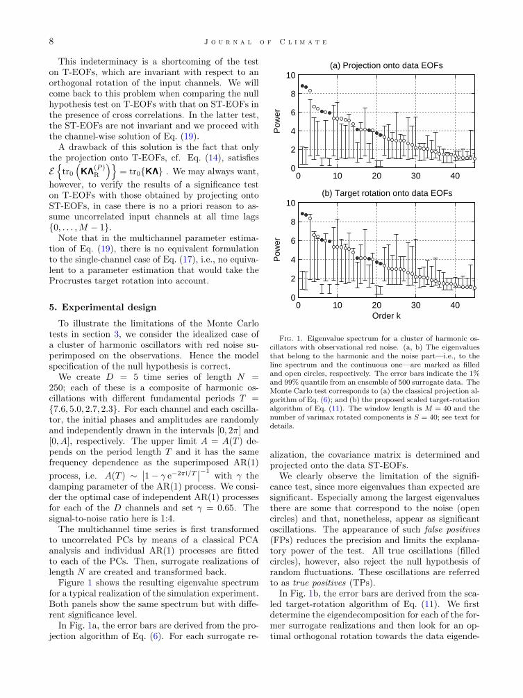
Figure 1 shows the resulting eigenvalue spectrumfor a typical realization of the simulation experiment.Both panels show the same spectrum but with diffe-rent significance level.
In Fig. 1a, the error bars are derived from the pro-jection algorithm of Eq. (6). For each surrogate re-
0 10 20 30 400
2
4
6
8
10
Pow
er
(a) Projection onto data EOFs
0 10 20 30 400
2
4
6
8
10
Order k
Pow
er
(b) Target rotation onto data EOFs
Fig. 1. Eigenvalue spectrum for a cluster of harmonic os-cillators with observational red noise. (a, b) The eigenvaluesthat belong to the harmonic and the noise part—i.e., to theline spectrum and the continuous one—are marked as filledand open circles, respectively. The error bars indicate the 1%and 99% quantile from an ensemble of 500 surrogate data. TheMonte Carlo test corresponds to (a) the classical projection al-gorithm of Eq. (6); and (b) the proposed scaled target-rotationalgorithm of Eq. (11). The window length is M = 40 and thenumber of varimax rotated components is S = 40; see text fordetails.
alization, the covariance matrix is determined andprojected onto the data ST-EOFs.
We clearly observe the limitation of the signifi-cance test, since more eigenvalues than expected aresignificant. Especially among the largest eigenvaluesthere are some that correspond to the noise (opencircles) and that, nonetheless, appear as significantoscillations. The appearance of such false positives(FPs) reduces the precision and limits the explana-tory power of the test. All true oscillations (filledcircles), however, also reject the null hypothesis ofrandom fluctuations. These oscillations are referredto as true positives (TPs).
In Fig. 1b, the error bars are derived from the sca-led target-rotation algorithm of Eq. (11). We firstdetermine the eigendecomposition for each of the for-mer surrogate realizations and then look for an op-timal orthogonal rotation towards the data eigende-
J o u r n a l o f C l i m a t e 9
0 0.1 0.2 0.3 0.4 0.510
−1
100
101
Projection onto EOFs of null hypothesisP
ower
Frequency (cycles/time unit)
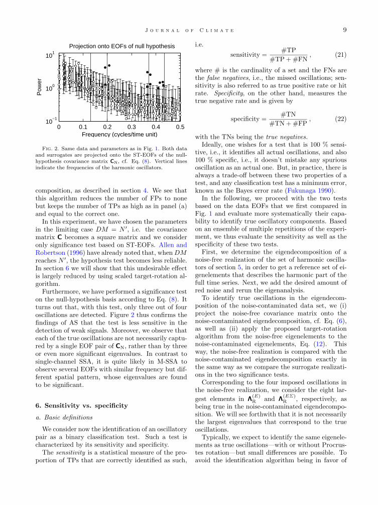
Fig. 2. Same data and parameters as in Fig. 1. Both dataand surrogates are projected onto the ST-EOFs of the null-hypothesis covariance matrix CN, cf. Eq. (8). Vertical linesindicate the frequencies of the harmonic oscillators.
composition, as described in section 4. We see thatthis algorithm reduces the number of FPs to nonebut keeps the number of TPs as high as in panel (a)and equal to the correct one.
In this experiment, we have chosen the parametersin the limiting case DM = N ′, i.e. the covariancematrix C becomes a square matrix and we consideronly significance test based on ST-EOFs. Allen andRobertson (1996) have already noted that, whenDMreaches N ′, the hypothesis test becomes less reliable.In section 6 we will show that this undesirable effectis largely reduced by using scaled target-rotation al-gorithm.
Furthermore, we have performed a significance teston the null-hypothesis basis according to Eq. (8). Itturns out that, with this test, only three out of fouroscillations are detected. Figure 2 thus confirms thefindings of AS that the test is less sensitive in thedetection of weak signals. Moreover, we observe thateach of the true oscillations are not necessarily captu-red by a single EOF pair of CN, rather than by threeor even more significant eigenvalues. In contrast tosingle-channel SSA, it is quite likely in M-SSA toobserve several EOFs with similar frequency but dif-ferent spatial pattern, whose eigenvalues are foundto be significant.
6. Sensitivity vs. specificity
a. Basic definitions
We consider now the identification of an oscillatorypair as a binary classification test. Such a test ischaracterized by its sensitivity and specificity.
The sensitivity is a statistical measure of the pro-portion of TPs that are correctly identified as such,
i.e.
sensitivity =#TP
#TP + #FN, (21)
where # is the cardinality of a set and the FNs arethe false negatives, i.e., the missed oscillations; sen-sitivity is also referred to as true positive rate or hitrate. Specificity, on the other hand, measures thetrue negative rate and is given by
specificity =#TN
#TN + #FP, (22)
with the TNs being the true negatives.Ideally, one wishes for a test that is 100 % sensi-
tive, i.e., it identifies all actual oscillations, and also100 % specific, i.e., it doesn’t mistake any spuriousoscillation as an actual one. But, in practice, there isalways a trade-off between these two properties of atest, and any classification test has a minimum error,known as the Bayes error rate (Fukunaga 1990).
In the following, we proceed with the two testsbased on the data EOFs that we first compared inFig. 1 and evaluate more systematically their capa-bility to identify true oscillatory components. Basedon an ensemble of multiple repetitions of the experi-ment, we thus evaluate the sensitivity as well as thespecificity of these two tests.
First, we determine the eigendecomposition of anoise-free realization of the set of harmonic oscilla-tors of section 5, in order to get a reference set of ei-genelements that describes the harmonic part of thefull time series. Next, we add the desired amount ofred noise and rerun the eigenanalysis.
To identify true oscillations in the eigendecom-position of the noise-contaminated data set, we (i)project the noise-free covariance matrix onto thenoise-contaminated eigendecomposition, cf. Eq. (6),as well as (ii) apply the proposed target-rotationalgorithm from the noise-free eigenelements to thenoise-contaminated eigenelements, Eq. (12). Thisway, the noise-free realization is compared with thenoise-contaminated eigendecomposition exactly inthe same way as we compare the surrogate realizati-ons in the two significance tests.
Corresponding to the four imposed oscillations inthe noise-free realization, we consider the eight lar-
gest elements in Λ(E)R and Λ
(EΣ)R , respectively, as
being true in the noise-contaminated eigendecompo-sition. We will see forthwith that it is not necessarilythe largest eigenvalues that correspond to the trueoscillations.
Typically, we expect to identify the same eigenele-ments as true oscillations—with or without Procrus-tes rotation—but small differences are possible. Toavoid the identification algorithm being in favor of
10 J o u r n a l o f C l i m a t e
0 10 20 30 400
0.2
0.4
0.6
0.8
1
Fre
quen
cy
Order k
(a) Specificity
ProjectionTarget rotation
0 10 20 30 400
0.2
0.4
0.6
0.8
1
Order k
Fre
quen
cy
(b) Distribution of true oscillations
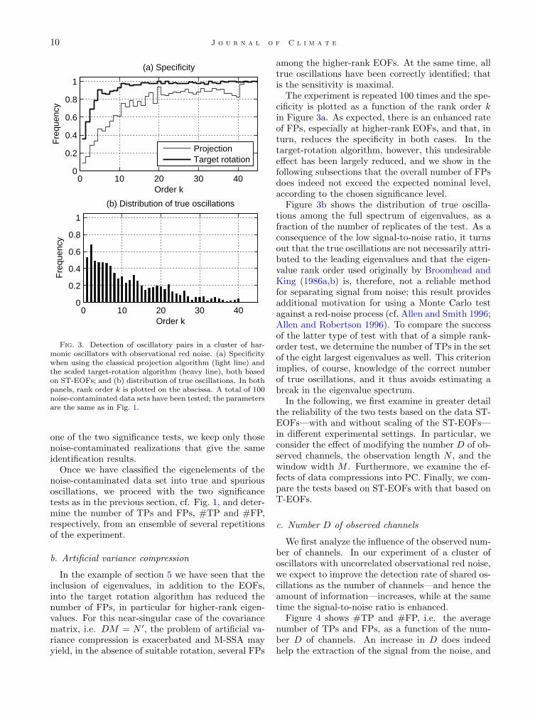
Fig. 3. Detection of oscillatory pairs in a cluster of har-monic oscillators with observational red noise. (a) Specificitywhen using the classical projection algorithm (light line) andthe scaled target-rotation algorithm (heavy line), both basedon ST-EOFs; and (b) distribution of true oscillations. In bothpanels, rank order k is plotted on the abscissa. A total of 100noise-contaminated data sets have been tested; the parametersare the same as in Fig. 1.
one of the two significance tests, we keep only thosenoise-contaminated realizations that give the sameidentification results.
Once we have classified the eigenelements of thenoise-contaminated data set into true and spuriousoscillations, we proceed with the two significancetests as in the previous section, cf. Fig. 1, and deter-mine the number of TPs and FPs, #TP and #FP,respectively, from an ensemble of several repetitionsof the experiment.
b. Artificial variance compression
In the example of section 5 we have seen that theinclusion of eigenvalues, in addition to the EOFs,into the target rotation algorithm has reduced thenumber of FPs, in particular for higher-rank eigen-values. For this near-singular case of the covariancematrix, i.e. DM = N ′, the problem of artificial va-riance compression is exacerbated and M-SSA mayyield, in the absence of suitable rotation, several FPs
among the higher-rank EOFs. At the same time, alltrue oscillations have been correctly identified; thatis the sensitivity is maximal.
The experiment is repeated 100 times and the spe-cificity is plotted as a function of the rank order kin Figure 3a. As expected, there is an enhanced rateof FPs, especially at higher-rank EOFs, and that, inturn, reduces the specificity in both cases. In thetarget-rotation algorithm, however, this undesirableeffect has been largely reduced, and we show in thefollowing subsections that the overall number of FPsdoes indeed not exceed the expected nominal level,according to the chosen significance level.
Figure 3b shows the distribution of true oscilla-tions among the full spectrum of eigenvalues, as afraction of the number of replicates of the test. As aconsequence of the low signal-to-noise ratio, it turnsout that the true oscillations are not necessarily attri-buted to the leading eigenvalues and that the eigen-value rank order used originally by Broomhead andKing (1986a,b) is, therefore, not a reliable methodfor separating signal from noise; this result providesadditional motivation for using a Monte Carlo testagainst a red-noise process (cf. Allen and Smith 1996;Allen and Robertson 1996). To compare the successof the latter type of test with that of a simple rank-order test, we determine the number of TPs in the setof the eight largest eigenvalues as well. This criterionimplies, of course, knowledge of the correct numberof true oscillations, and it thus avoids estimating abreak in the eigenvalue spectrum.
In the following, we first examine in greater detailthe reliability of the two tests based on the data ST-EOFs—with and without scaling of the ST-EOFs—in different experimental settings. In particular, weconsider the effect of modifying the number D of ob-served channels, the observation length N , and thewindow width M . Furthermore, we examine the ef-fects of data compressions into PC. Finally, we com-pare the tests based on ST-EOFs with that based onT-EOFs.
c. Number D of observed channels
We first analyze the influence of the observed num-ber of channels. In our experiment of a cluster ofoscillators with uncorrelated observational red noise,we expect to improve the detection rate of shared os-cillations as the number of channels—and hence theamount of information—increases, while at the sametime the signal-to-noise ratio is enhanced.
Figure 4 shows #TP and #FP, i.e. the averagenumber of TPs and FPs, as a function of the num-ber D of channels. An increase in D does indeedhelp the extraction of the signal from the noise, and

J o u r n a l o f C l i m a t e 11
D
# F
P
| #
TP
N = 250 | M = 40
1 2 3 4 5 6 7 8 9 10 11 120
1
2
3
4
5
6
7
8
9
10
11
#TP unscaled
#TP scaled
#FP unscaled
#FP scaled
Fig. 4. Detection of oscillations in a cluster of harmonicoscillators with observational red noise. The average numberof true positives (#TP) and false positives (#FP) is plotted,along with the corresponding standard deviation (error bars),based on an ensemble of 50 repetitions of the experiment, asthe number D of observed channels increases. The parame-ters M and N are the same as in Fig. 1. The dashed linescorrespond to the unscaled target-rotation algorithm onto ST-EOFs and the solid lines to the scaled one. The former inclu-des the projection algorithm as a special case for DM ≤ N ′.A black bar along the horizontal axis indicates the D-intervalwithin which the covariance matrix C becomes rank-deficient,DM > N ′. In addition, the average number of TPs withinthe set of the eight largest eigenvalues (heavy gray line), andthe expected number of FPs according to the significance level(gray shaded area) are shown.
the number of TPs converges toward its maximumvalue, which is max{#TP} = 8 in case of the fourfundamental frequencies T = {7.6, 5.0, 2.7, 2.3}.
The convergence occurs already for D = 5, while insingle-channel SSA, i.e. for D = 1 in the figure, onlyhalf of the oscillations have been identified. This re-sult clearly illustrates the fact that M-SSA improvesupon single-channel SSA by taking additional spatialinformation into account.
This improved detection rate, however, cannot bemerely attributed to a concentration of oscillatorybehavior in the largest eigenvalues alone. It turns outthat no more than half of the eight largest eigenvaluesare TPs (heavy gray line in Fig. 4).
While the sensitivity of the test does grow with D,it is indispensable to keep the specificity high as well.Figure 4 makes it clear that this is not the case for theprojection algorithm, i.e. when DM ≤ N ′, in whichthe number of FPs (red dashed line) increases as well.
In particular, #FP greatly exceeds the number ofexpected FPs (gray shaded area), which equals thenumber of eigenvalues multiplied by the significancelevel. This excess of type-I error becomes more dra-matic as one approaches the point at which the cova-riance matrix C reaches rank deficiency, DM . N ′.For DM > N ′, i.e. the unscaled target-rotation al-gorithm, the number of FPs remains likewise high,and reaches nearly the number of TPs. This ren-ders the test useless, since only half of the significanteigenvalues can be attributed to true oscillations.
It is only the inclusion of eigenvalue informationinto the scaled target-rotation algorithm that finallyhelps control this type-I error, with the average num-ber of FPs (solid red line in Fig. 4) now below the ex-pected level of FPs over the entire range of D-values.We note that this algorithm has a slight tendencytowards a more conservative behavior—a propertythat Procrustes methods have been often criticizedfor (e.g., Paunonen 1997)—but the detection rateremains comparable to that of the unscaled target-rotation algorithm. In particular, the scaled target-rotation algorithm would be the preferable choicewith respect to the test’s explanatory power.
To improve the detection of weak signals in thecase of single-channel SSA, Palus and Novotna(2004) proposed a test on the regularity of the os-cillatory modes rather than on their variance. Theirsignificance test has a demonstrably enhanced sen-sitivity, but it is not clear whether it remains suffi-ciently specific as well; see, for instance Figs. 2 and4 in Palus and Novotna (2004), with further “noise”EOFs becoming significant above the upper signifi-cance levels in the test on regularity. On the otherhand, the frequency-pairing algorithm in their testis much less susceptible to the problem of artificialvariance compression than the projection approachin Eq. (6); see again their Fig. 2, with the number ofsignificant “noise” EOFs below the lower significancelevels becoming largely reduced.
d. Length N of the observations
In the previous subsection we have seen that forthe unscaled target-rotation algorithm, the specifi-city strongly depends on the ratio of the embeddingdimension DM to the time series length N . It is thesingular character of the covariance matrix C that en-hances the artificial variance compression, and thusgives a high number of FPs in this algorithm. We ex-amine next whether this undesirable property can beavoided when the observation length N considerablyexceeds (D + 1)M for fixed M .
For a fixed number D of channels, we have variedthe observation length N and rerun the analysis as
12 J o u r n a l o f C l i m a t e
N
# F
P
| #
TP
D = 5 | M = 40
80 100 150 200 300 400 6000
1
2
3
4
5
6
7
8
#TP unscaled
#TP scaled
#FP unscaled
#FP scaled
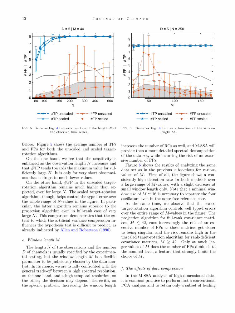
Fig. 5. Same as Fig. 4 but as a function of the length N ofthe observed time series.
before. Figure 5 shows the average number of TPsand FPs for both the unscaled and scaled target-rotation algorithms.
On the one hand, we see that the sensitivity isenhanced as the observation length N increases andthat #TP tends towards the maximum value for suf-ficiently large N . It is only for very short observati-ons that it drops to much lower values.
On the other hand, #FP in the unscaled target-rotation algorithm remains much higher than ex-pected, even for large N . The scaled target-rotationalgorithm, though, helps control the type I-error overthe whole range of N -values in the figure. In parti-cular, the latter algorithm remains superior to theprojection algorithm even in full-rank case of verylarge N . This comparison demonstrates that the ex-tent to which the artificial variance compression in-fluences the hypothesis test is difficult to predict, asalready indicated by Allen and Robertson (1996).
e. Window length M
The length N of the observations and the numberD of channels is usually specified by the experimen-tal setting, but the window length M is a flexibleparameter to be judiciously chosen by the data ana-lyst. In its choice, we are usually confronted with thegeneral trade-off between a high spectral resolution,on the one hand, and a high temporal resolution, onthe other; the decision may depend, therewith, onthe specific problem. Increasing the window length
M
# F
P
| #
TP
D = 5 | N = 250
50 100 1500
1
2
3
4
5
6
7
8
9
#TP unscaled
#TP scaled
#FP unscaled
#FP scaled
Fig. 6. Same as Fig. 4 but as a function of the windowlength M .
increases the number of RCs as well, and M-SSA willprovide then a more detailed spectral decompositionof the data set, while incurring the risk of an exces-sive number of FPs.
Figure 6 shows the results of analyzing the samedata set as in the previous subsections for variousvalues of M . First of all, the figure shows a con-sistently high detection rate for both methods overa large range of M -values, with a slight decrease atsmall window length only. Note that a minimal win-dow size of M ' 16 is necessary to separate the fouroscillators even in the noise-free reference case.
At the same time, we observe that the scaledtarget-rotation algorithm controls well type-I errorsover the entire range of M -values in the figure. Theprojection algorithm for full-rank covariance matri-ces, M . 42, runs increasingly the risk of an ex-cessive number of FPs as these matrices get closerto being singular, and the risk remains high in theunscaled target-rotation algorithm for rank-deficientcovariance matrices, M ≥ 42. Only at much lar-ger values of M does the number of FPs diminish tothe nominal level, a feature that strongly limits thechoice of M .
f. The effects of data compression
In the M-SSA analysis of high-dimensional data,it is common practice to perform first a conventionalPCA analysis and to retain only a subset of leading
J o u r n a l o f C l i m a t e 13
PCs for the subsequent M-SSA analysis. This pre-processing is meant to reduce the number of inputchannels and the computational cost, while retaininga large fraction of the total variance. Usually a smallnumber L of channels is kept, no matter how largethe data set (Dettinger et al. 1995; Allen and Robert-son 1996; Robertson 1996; Ghil et al. 2002b); see also(Moron et al. 1998, Table 1). Since the resulting PCsare pairwise uncorrelated at zero lag, the M-SSA re-sults can be simply tested against independent AR(1)processes, cf. section 3 herein.
Even though the transformation to conventionalPCs turns out to be a helpful preprocessing stepin the M-SSA analysis, its implications for the pro-perties of the subsequent signal detection are rathercomplex. Given that the signal of interest involvestypically only a small fraction of the total variance,we would expect it to show up only among the spatialEOFs (S-EOFs) with relatively small variance, whilethe leading S-EOFs might capture other large-scaleeffects. In this respect, the prior transformation toPCs could interfere with the detection of weak sig-nals.
To study the implications of this type of prepro-cessing, we increase the number of observed channelsin the previous example of a cluster of harmonic os-cillators to D = 250 and reduce at the same timethe observation length to N = 130. The parameter γfor the D superimposed AR(1) processes is randomlydrawn from the interval γ ∈ [0, 0.95], but we intro-duce at the same time correlations between all ofthem. That is, instead of adding independent noiserealizations to each of the observed channels, we setthe lag-0 covariance matrix W of the noise part to fita Toeplitz structure, with Wij = κ|i−j| and κ = 0.5.
These correlations between channels are meant tosimulate the effect of spatial correlations in a rand-omly perturbed spatio-temporal process and, givenour choice of κ, we expect the noise part to domi-nate the prior PCA analysis.
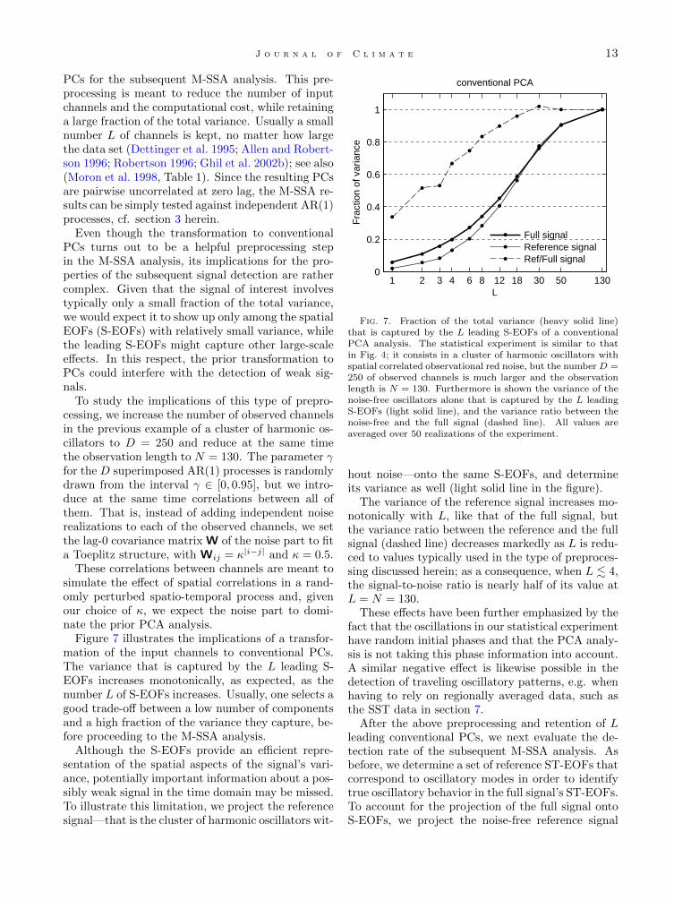
Figure 7 illustrates the implications of a transfor-mation of the input channels to conventional PCs.The variance that is captured by the L leading S-EOFs increases monotonically, as expected, as thenumber L of S-EOFs increases. Usually, one selects agood trade-off between a low number of componentsand a high fraction of the variance they capture, be-fore proceeding to the M-SSA analysis.
Although the S-EOFs provide an efficient repre-sentation of the spatial aspects of the signal’s vari-ance, potentially important information about a pos-sibly weak signal in the time domain may be missed.To illustrate this limitation, we project the referencesignal—that is the cluster of harmonic oscillators wit-
1 2 3 4 6 8 12 18 30 50 1300
0.2
0.4
0.6
0.8
1
L
Fra
ctio
n of
var
ianc
e
conventional PCA
Full signalReference signalRef/Full signal
Fig. 7. Fraction of the total variance (heavy solid line)that is captured by the L leading S-EOFs of a conventionalPCA analysis. The statistical experiment is similar to thatin Fig. 4; it consists in a cluster of harmonic oscillators withspatial correlated observational red noise, but the number D =250 of observed channels is much larger and the observationlength is N = 130. Furthermore is shown the variance of thenoise-free oscillators alone that is captured by the L leadingS-EOFs (light solid line), and the variance ratio between thenoise-free and the full signal (dashed line). All values areaveraged over 50 realizations of the experiment.
hout noise—onto the same S-EOFs, and determineits variance as well (light solid line in the figure).
The variance of the reference signal increases mo-notonically with L, like that of the full signal, butthe variance ratio between the reference and the fullsignal (dashed line) decreases markedly as L is redu-ced to values typically used in the type of preproces-sing discussed herein; as a consequence, when L . 4,the signal-to-noise ratio is nearly half of its value atL = N = 130.
These effects have been further emphasized by thefact that the oscillations in our statistical experimenthave random initial phases and that the PCA analy-sis is not taking this phase information into account.A similar negative effect is likewise possible in thedetection of traveling oscillatory patterns, e.g. whenhaving to rely on regionally averaged data, such asthe SST data in section 7.
After the above preprocessing and retention of Lleading conventional PCs, we next evaluate the de-tection rate of the subsequent M-SSA analysis. Asbefore, we determine a set of reference ST-EOFs thatcorrespond to oscillatory modes in order to identifytrue oscillatory behavior in the full signal’s ST-EOFs.To account for the projection of the full signal ontoS-EOFs, we project the noise-free reference signal
14 J o u r n a l o f C l i m a t e
L
# F
P
| #
TP
N = 130 | M = 40 | D = 250
1 2 6 12 30 50 1300
1
2
3
4
5
6
7
8
#TP scaled #FP scaled
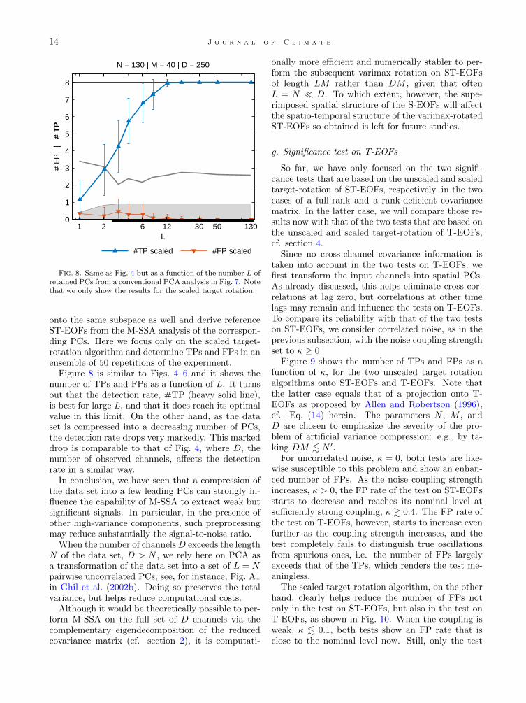
Fig. 8. Same as Fig. 4 but as a function of the number L ofretained PCs from a conventional PCA analysis in Fig. 7. Notethat we only show the results for the scaled target rotation.
onto the same subspace as well and derive referenceST-EOFs from the M-SSA analysis of the correspon-ding PCs. Here we focus only on the scaled target-rotation algorithm and determine TPs and FPs in anensemble of 50 repetitions of the experiment.
Figure 8 is similar to Figs. 4–6 and it shows thenumber of TPs and FPs as a function of L. It turnsout that the detection rate, #TP (heavy solid line),is best for large L, and that it does reach its optimalvalue in this limit. On the other hand, as the dataset is compressed into a decreasing number of PCs,the detection rate drops very markedly. This markeddrop is comparable to that of Fig. 4, where D, thenumber of observed channels, affects the detectionrate in a similar way.
In conclusion, we have seen that a compression ofthe data set into a few leading PCs can strongly in-fluence the capability of M-SSA to extract weak butsignificant signals. In particular, in the presence ofother high-variance components, such preprocessingmay reduce substantially the signal-to-noise ratio.
When the number of channelsD exceeds the lengthN of the data set, D > N , we rely here on PCA asa transformation of the data set into a set of L = Npairwise uncorrelated PCs; see, for instance, Fig. A1in Ghil et al. (2002b). Doing so preserves the totalvariance, but helps reduce computational costs.
Although it would be theoretically possible to per-form M-SSA on the full set of D channels via thecomplementary eigendecomposition of the reducedcovariance matrix (cf. section 2), it is computati-
onally more efficient and numerically stabler to per-form the subsequent varimax rotation on ST-EOFsof length LM rather than DM , given that oftenL = N � D. To which extent, however, the supe-rimposed spatial structure of the S-EOFs will affectthe spatio-temporal structure of the varimax-rotatedST-EOFs so obtained is left for future studies.
g. Significance test on T-EOFs
So far, we have only focused on the two signifi-cance tests that are based on the unscaled and scaledtarget-rotation of ST-EOFs, respectively, in the twocases of a full-rank and a rank-deficient covariancematrix. In the latter case, we will compare those re-sults now with that of the two tests that are based onthe unscaled and scaled target-rotation of T-EOFs;cf. section 4.
Since no cross-channel covariance information istaken into account in the two tests on T-EOFs, wefirst transform the input channels into spatial PCs.As already discussed, this helps eliminate cross cor-relations at lag zero, but correlations at other timelags may remain and influence the tests on T-EOFs.To compare its reliability with that of the two testson ST-EOFs, we consider correlated noise, as in theprevious subsection, with the noise coupling strengthset to κ ≥ 0.
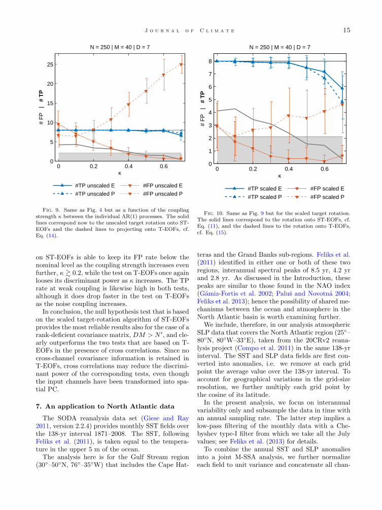
Figure 9 shows the number of TPs and FPs as afunction of κ, for the two unscaled target rotationalgorithms onto ST-EOFs and T-EOFs. Note thatthe latter case equals that of a projection onto T-EOFs as proposed by Allen and Robertson (1996),cf. Eq. (14) herein. The parameters N , M , andD are chosen to emphasize the severity of the pro-blem of artificial variance compression: e.g., by ta-king DM . N ′.
For uncorrelated noise, κ = 0, both tests are like-wise susceptible to this problem and show an enhan-ced number of FPs. As the noise coupling strengthincreases, κ > 0, the FP rate of the test on ST-EOFsstarts to decrease and reaches its nominal level atsufficiently strong coupling, κ & 0.4. The FP rate ofthe test on T-EOFs, however, starts to increase evenfurther as the coupling strength increases, and thetest completely fails to distinguish true oscillationsfrom spurious ones, i.e. the number of FPs largelyexceeds that of the TPs, which renders the test me-aningless.
The scaled target-rotation algorithm, on the otherhand, clearly helps reduce the number of FPs notonly in the test on ST-EOFs, but also in the test onT-EOFs, as shown in Fig. 10. When the coupling isweak, κ . 0.1, both tests show an FP rate that isclose to the nominal level now. Still, only the test
J o u r n a l o f C l i m a t e 15
κ
# F
P
| #
TP
N = 250 | M = 40 | D = 7
0 0.2 0.4 0.60
5
10
15
20
25
#TP unscaled E
#TP unscaled P
#FP unscaled E
#FP unscaled P
Fig. 9. Same as Fig. 4 but as a function of the couplingstrength κ between the individual AR(1) processes. The solidlines correspond now to the unscaled target rotation onto ST-EOFs and the dashed lines to projecting onto T-EOFs, cf.Eq. (14).
on ST-EOFs is able to keep its FP rate below thenominal level as the coupling strength increases evenfurther, κ & 0.2, while the test on T-EOFs once againlooses its discriminant power as κ increases. The TPrate at weak coupling is likewise high in both tests,although it does drop faster in the test on T-EOFsas the noise coupling increases.
In conclusion, the null hypothesis test that is basedon the scaled target-rotation algorithm of ST-EOFsprovides the most reliable results also for the case of arank-deficient covariance matrix, DM > N ′, and cle-arly outperforms the two tests that are based on T-EOFs in the presence of cross correlations. Since nocross-channel covariance information is retained inT-EOFs, cross correlations may reduce the discrimi-nant power of the corresponding tests, even thoughthe input channels have been transformed into spa-tial PC.
7. An application to North Atlantic data
The SODA reanalysis data set (Giese and Ray2011, version 2.2.4) provides monthly SST fields overthe 138-yr interval 1871–2008. The SST, followingFeliks et al. (2011), is taken equal to the tempera-ture in the upper 5 m of the ocean.
The analysis here is for the Gulf Stream region(30◦–50◦N, 76◦–35◦W) that includes the Cape Hat-
κ
# F
P
| #
TP
N = 250 | M = 40 | D = 7
0 0.2 0.4 0.60
1
2
3
4
5
6
7
8
#TP scaled E
#TP scaled P
#FP scaled E
#FP scaled P
Fig. 10. Same as Fig. 9 but for the scaled target rotation.The solid lines correspond to the rotation onto ST-EOFs, cf.Eq. (11), and the dashed lines to the rotation onto T-EOFs,cf. Eq. (15).
teras and the Grand Banks sub-regions. Feliks et al.(2011) identified in either one or both of these tworegions, interannual spectral peaks of 8.5 yr, 4.2 yrand 2.8 yr. As discussed in the Introduction, thesepeaks are similar to those found in the NAO index(Gamiz-Fortis et al. 2002; Palus and Novotna 2004;Feliks et al. 2013); hence the possibility of shared me-chanisms between the ocean and atmosphere in theNorth Atlantic basin is worth examining further.
We include, therefore, in our analysis atmosphericSLP data that covers the North Atlantic region (25◦–80◦N, 80◦W–33◦E), taken from the 20CRv2 reana-lysis project (Compo et al. 2011) in the same 138-yrinterval. The SST and SLP data fields are first con-verted into anomalies, i.e. we remove at each gridpoint the average value over the 138-yr interval. Toaccount for geographical variations in the grid-sizeresolution, we further multiply each grid point bythe cosine of its latitude.
In the present analysis, we focus on interannualvariability only and subsample the data in time withan annual sampling rate. The latter step implies alow-pass filtering of the monthly data with a Che-byshev type-I filter from which we take all the Julyvalues; see Feliks et al. (2013) for details.
To combine the annual SST and SLP anomaliesinto a joint M-SSA analysis, we further normalizeeach field to unit variance and concatenate all chan-
16 J o u r n a l o f C l i m a t e
0 0.1 0.2 0.3 0.4 0.510
−1
100
Frequency (cycles/year)
Pow
er(a) Target rotation onto data ST−EOFs
0 0.1 0.2 0.3 0.4 0.510
−1
100
Frequency (cycles/year)
Pow
er
(b) Projection onto null hypothesis T−EOFs
1880 1900 1920 1940 1960 1980 2000−100
0
100(c) RCs 1−3 | 22.9%
Pa
Year
−1
0
1
°C
SLP SST
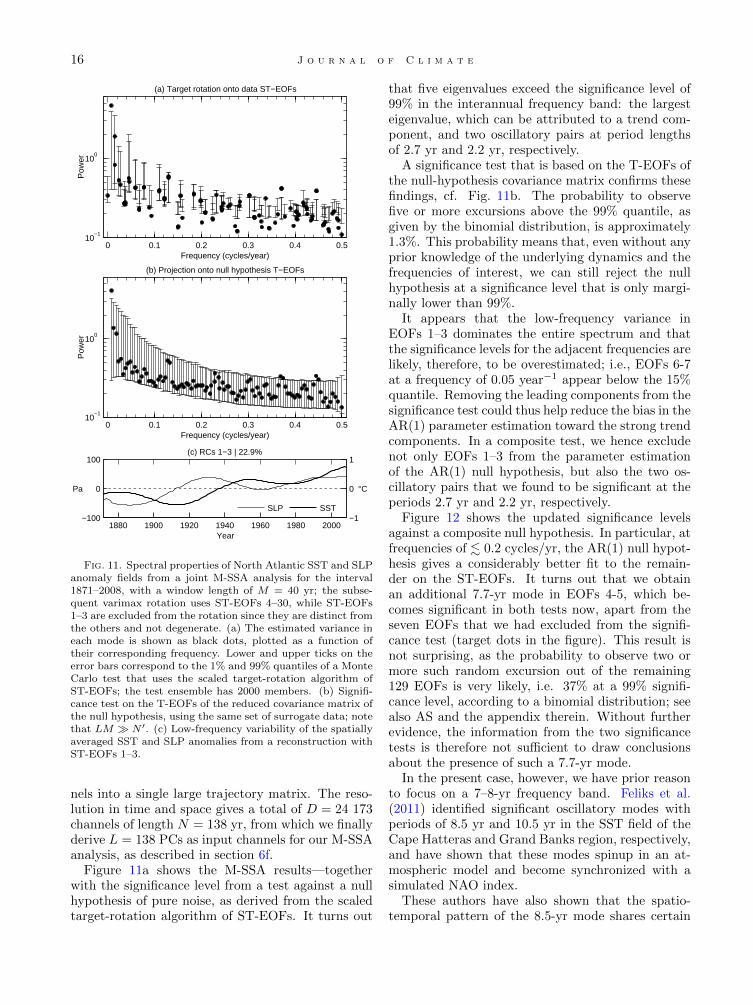
Fig. 11. Spectral properties of North Atlantic SST and SLPanomaly fields from a joint M-SSA analysis for the interval1871–2008, with a window length of M = 40 yr; the subse-quent varimax rotation uses ST-EOFs 4–30, while ST-EOFs1–3 are excluded from the rotation since they are distinct fromthe others and not degenerate. (a) The estimated variance ineach mode is shown as black dots, plotted as a function oftheir corresponding frequency. Lower and upper ticks on theerror bars correspond to the 1% and 99% quantiles of a MonteCarlo test that uses the scaled target-rotation algorithm ofST-EOFs; the test ensemble has 2000 members. (b) Signifi-cance test on the T-EOFs of the reduced covariance matrix ofthe null hypothesis, using the same set of surrogate data; notethat LM � N ′. (c) Low-frequency variability of the spatiallyaveraged SST and SLP anomalies from a reconstruction withST-EOFs 1–3.
nels into a single large trajectory matrix. The reso-lution in time and space gives a total of D = 24 173channels of length N = 138 yr, from which we finallyderive L = 138 PCs as input channels for our M-SSAanalysis, as described in section 6f.
Figure 11a shows the M-SSA results—togetherwith the significance level from a test against a nullhypothesis of pure noise, as derived from the scaledtarget-rotation algorithm of ST-EOFs. It turns out
that five eigenvalues exceed the significance level of99% in the interannual frequency band: the largesteigenvalue, which can be attributed to a trend com-ponent, and two oscillatory pairs at period lengthsof 2.7 yr and 2.2 yr, respectively.
A significance test that is based on the T-EOFs ofthe null-hypothesis covariance matrix confirms thesefindings, cf. Fig. 11b. The probability to observefive or more excursions above the 99% quantile, asgiven by the binomial distribution, is approximately1.3%. This probability means that, even without anyprior knowledge of the underlying dynamics and thefrequencies of interest, we can still reject the nullhypothesis at a significance level that is only margi-nally lower than 99%.
It appears that the low-frequency variance inEOFs 1–3 dominates the entire spectrum and thatthe significance levels for the adjacent frequencies arelikely, therefore, to be overestimated; i.e., EOFs 6-7at a frequency of 0.05 year−1 appear below the 15%quantile. Removing the leading components from thesignificance test could thus help reduce the bias in theAR(1) parameter estimation toward the strong trendcomponents. In a composite test, we hence excludenot only EOFs 1–3 from the parameter estimationof the AR(1) null hypothesis, but also the two os-cillatory pairs that we found to be significant at theperiods 2.7 yr and 2.2 yr, respectively.
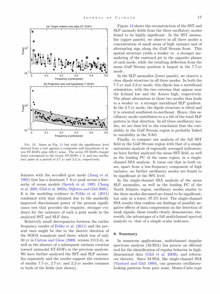
Figure 12 shows the updated significance levelsagainst a composite null hypothesis. In particular, atfrequencies of . 0.2 cycles/yr, the AR(1) null hypot-hesis gives a considerably better fit to the remain-der on the ST-EOFs. It turns out that we obtainan additional 7.7-yr mode in EOFs 4-5, which be-comes significant in both tests now, apart from theseven EOFs that we had excluded from the signifi-cance test (target dots in the figure). This result isnot surprising, as the probability to observe two ormore such random excursion out of the remaining129 EOFs is very likely, i.e. 37% at a 99% signifi-cance level, according to a binomial distribution; seealso AS and the appendix therein. Without furtherevidence, the information from the two significancetests is therefore not sufficient to draw conclusionsabout the presence of such a 7.7-yr mode.
In the present case, however, we have prior reasonto focus on a 7–8-yr frequency band. Feliks et al.(2011) identified significant oscillatory modes withperiods of 8.5 yr and 10.5 yr in the SST field of theCape Hatteras and Grand Banks region, respectively,and have shown that these modes spinup in an at-mospheric model and become synchronized with asimulated NAO index.
These authors have also shown that the spatio-temporal pattern of the 8.5-yr mode shares certain
J o u r n a l o f C l i m a t e 17
0 0.1 0.2 0.3 0.4 0.510
−1
100
Frequency (cycles/year)
Pow
er(a) Target rotation onto data ST−EOFs
0 0.1 0.2 0.3 0.4 0.510
−1
100
Frequency (cycles/year)
Pow
er
(b) Projection onto null hypothesis T−EOFs
Fig. 12. Same as Fig. 11 but with the significance levelderived from a test against a composite null hypothesis of se-ven ST-EOFs plus AR(1) noise. The seven ST-EOFs (targetdots) correspond to the trend, ST-EOFs 1–3, and two oscilla-tory pairs at a period of 2.7 yr and 2.2 yr, respectively.
features with the so-called gyre mode (Jiang et al.1995) that has a dominant 7–8-yr peak across a hier-archy of ocean models (Speich et al. 1995; Changet al. 2001; Ghil et al. 2002a; Dijkstra and Ghil 2005).It is the modeling evidence in Feliks et al. (2011)combined with that obtained due to the markedlyimproved discriminant power of the present signifi-cance test that provides the requisite, stronger evi-dence for the existence of such a joint mode in theanalyzed SST and SLP data.
Relatively small discrepancies between the earlierfrequency results of Feliks et al. (2011) and the pre-sent ones might be due to the shorter duration ofthe SODA reanalysis used there, which was of only50 yr in Carton and Giese (2008, version 2.0.2-4), aswell as the absence of a subsequent varimax rotationtoward unimodal ST-EOFs in the previous analysis.We have further analyzed the SST and SLP anoma-lies separately and the results support the existenceof similar 7.7-yr, 2.7-yr, and 2.2-yr modes commonto both of the fields (not shown).
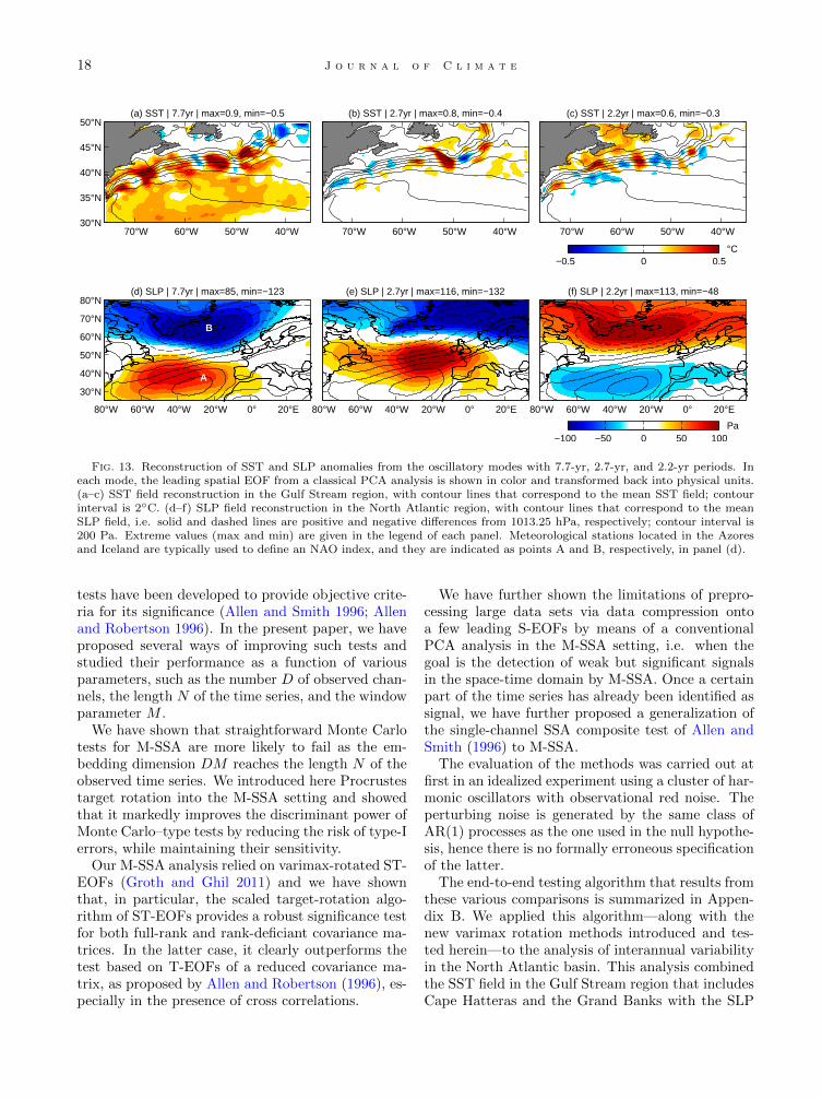
Figure 13 shows the reconstruction of the SST andSLP anomaly fields from the three oscillatory modesfound to be highly significant. In the SST anoma-lies (upper panels), we observe in all three modes aconcentration of small areas of high variance and ofalternating sign along the Gulf Stream front. Thisspatial structure yields a weaker vs. a stronger me-andering of the eastward jet in the opposite phasesof each mode, while the resulting deflection from themean Gulf Stream position is largest in the 7.7-yrmode.
In the SLP anomalies (lower panels), we observe aclear dipole structure in all three modes. In both the7.7-yr and 2.2-yr mode, this dipole has a meridionalorientation, with the two extrema that appear nearthe Iceland low and the Azores high, respectively.The phase alternation in these two modes thus leadsto a weaker vs. a stronger meridional SLP gradient.In the 2.7-yr mode, the dipole structure is tilted andit is oriented southwest-to-northeast. Hence, this os-cillatory mode contributes to a a tilt of the total SLPpattern in that direction. In all three oscillatory mo-des, we are thus led to the conclusion that the vari-ability in the Gulf Stream region is probably linkedto variability in the NAO.
Finally, to compare our analysis of the full SSTfield in the Gulf Stream region with that of a simpleunivariate analysis of regionally averaged indicators,we have further analyzed the mean SST field, as wellas the leading PC of the same region, in a single-channel SSA analysis. It turns out that in both ca-ses, apart from a low-frequency component of highvariance, no further oscillatory modes are found tobe significant at the 99% level.
In the single-channel SSA analysis of the meanSLP anomalies, as well as the leading PC of theNorth Atlantic region, oscillatory modes similar tothe three modes discussed are found to be significant,but only at a lower, 97.5% level. The single-channelSSA results thus confirm our findings of possibly ne-gative effects of data compression on the detection ofweak signals; these results clearly demonstrate, the-rewith, the advantages of a full multichannel spectralanalysis vs. that of a simple scalar indicator.
8. Summary
In numerous applications, multichannel singularspectrum analysis (M-SSA) has proven an efficienttool for the identification of regular behavior in high-dimensional data (Ghil et al. 2002b, and referen-ces therein). Since M-SSA, like single-channel SSA(Vautard and Ghil 1989), can generate oscillatory-looking patterns from pure noise, Monte-Carlo type
18 J o u r n a l o f C l i m a t e
(a) SST | 7.7yr | max=0.9, min=−0.5
H
70°W 60°W 50°W 40°W 30°N
35°N
40°N
45°N
50°N(b) SST | 2.7yr | max=0.8, min=−0.4
70°W 60°W 50°W 40°W
(c) SST | 2.2yr | max=0.6, min=−0.3
70°W 60°W 50°W 40°W
°C−0.5 0 0.5
(d) SLP | 7.7yr | max=85, min=−123
A
B
80°W 60°W 40°W 20°W 0° 20°E
30°N
40°N
50°N
60°N
70°N
80°N(e) SLP | 2.7yr | max=116, min=−132
80°W 60°W 40°W 20°W 0° 20°E
(f) SLP | 2.2yr | max=113, min=−48
80°W 60°W 40°W 20°W 0° 20°E
Pa−100 −50 0 50 100
Fig. 13. Reconstruction of SST and SLP anomalies from the oscillatory modes with 7.7-yr, 2.7-yr, and 2.2-yr periods. Ineach mode, the leading spatial EOF from a classical PCA analysis is shown in color and transformed back into physical units.(a–c) SST field reconstruction in the Gulf Stream region, with contour lines that correspond to the mean SST field; contourinterval is 2◦C. (d–f) SLP field reconstruction in the North Atlantic region, with contour lines that correspond to the meanSLP field, i.e. solid and dashed lines are positive and negative differences from 1013.25 hPa, respectively; contour interval is200 Pa. Extreme values (max and min) are given in the legend of each panel. Meteorological stations located in the Azoresand Iceland are typically used to define an NAO index, and they are indicated as points A and B, respectively, in panel (d).
tests have been developed to provide objective crite-ria for its significance (Allen and Smith 1996; Allenand Robertson 1996). In the present paper, we haveproposed several ways of improving such tests andstudied their performance as a function of variousparameters, such as the number D of observed chan-nels, the length N of the time series, and the windowparameter M .
We have shown that straightforward Monte Carlotests for M-SSA are more likely to fail as the em-bedding dimension DM reaches the length N of theobserved time series. We introduced here Procrustestarget rotation into the M-SSA setting and showedthat it markedly improves the discriminant power ofMonte Carlo–type tests by reducing the risk of type-Ierrors, while maintaining their sensitivity.
Our M-SSA analysis relied on varimax-rotated ST-EOFs (Groth and Ghil 2011) and we have shownthat, in particular, the scaled target-rotation algo-rithm of ST-EOFs provides a robust significance testfor both full-rank and rank-deficiant covariance ma-trices. In the latter case, it clearly outperforms thetest based on T-EOFs of a reduced covariance ma-trix, as proposed by Allen and Robertson (1996), es-pecially in the presence of cross correlations.
We have further shown the limitations of prepro-cessing large data sets via data compression ontoa few leading S-EOFs by means of a conventionalPCA analysis in the M-SSA setting, i.e. when thegoal is the detection of weak but significant signalsin the space-time domain by M-SSA. Once a certainpart of the time series has already been identified assignal, we have further proposed a generalization ofthe single-channel SSA composite test of Allen andSmith (1996) to M-SSA.
The evaluation of the methods was carried out atfirst in an idealized experiment using a cluster of har-monic oscillators with observational red noise. Theperturbing noise is generated by the same class ofAR(1) processes as the one used in the null hypothe-sis, hence there is no formally erroneous specificationof the latter.
The end-to-end testing algorithm that results fromthese various comparisons is summarized in Appen-dix B. We applied this algorithm—along with thenew varimax rotation methods introduced and tes-ted herein—to the analysis of interannual variabilityin the North Atlantic basin. This analysis combinedthe SST field in the Gulf Stream region that includesCape Hatteras and the Grand Banks with the SLP
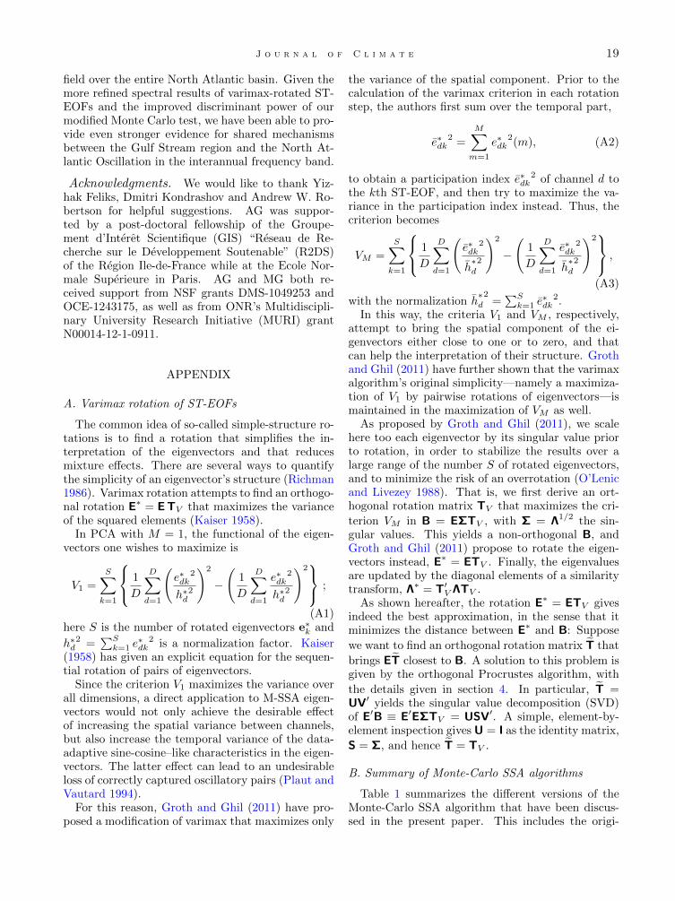
J o u r n a l o f C l i m a t e 19
field over the entire North Atlantic basin. Given themore refined spectral results of varimax-rotated ST-EOFs and the improved discriminant power of ourmodified Monte Carlo test, we have been able to pro-vide even stronger evidence for shared mechanismsbetween the Gulf Stream region and the North At-lantic Oscillation in the interannual frequency band.
Acknowledgments. We would like to thank Yiz-hak Feliks, Dmitri Kondrashov and Andrew W. Ro-bertson for helpful suggestions. AG was suppor-ted by a post-doctoral fellowship of the Groupe-ment d’Interet Scientifique (GIS) “Reseau de Re-cherche sur le Developpement Soutenable” (R2DS)of the Region Ile-de-France while at the Ecole Nor-male Superieure in Paris. AG and MG both re-ceived support from NSF grants DMS-1049253 andOCE-1243175, as well as from ONR’s Multidiscipli-nary University Research Initiative (MURI) grantN00014-12-1-0911.
APPENDIX
A. Varimax rotation of ST-EOFs
The common idea of so-called simple-structure ro-tations is to find a rotation that simplifies the in-terpretation of the eigenvectors and that reducesmixture effects. There are several ways to quantifythe simplicity of an eigenvector’s structure (Richman1986). Varimax rotation attempts to find an orthogo-nal rotation E∗ = E TV that maximizes the varianceof the squared elements (Kaiser 1958).
In PCA with M = 1, the functional of the eigen-vectors one wishes to maximize is
V1 =S∑k=1
1
D
D∑d=1
(e∗dk
2
h∗d2
)2
−(
1
D
D∑d=1
e∗dk2
h∗d2
)2 ;
(A1)here S is the number of rotated eigenvectors e∗k and
h∗d2 =
∑Sk=1 e
∗dk
2 is a normalization factor. Kaiser(1958) has given an explicit equation for the sequen-tial rotation of pairs of eigenvectors.
Since the criterion V1 maximizes the variance overall dimensions, a direct application to M-SSA eigen-vectors would not only achieve the desirable effectof increasing the spatial variance between channels,but also increase the temporal variance of the data-adaptive sine-cosine–like characteristics in the eigen-vectors. The latter effect can lead to an undesirableloss of correctly captured oscillatory pairs (Plaut andVautard 1994).
For this reason, Groth and Ghil (2011) have pro-posed a modification of varimax that maximizes only
the variance of the spatial component. Prior to thecalculation of the varimax criterion in each rotationstep, the authors first sum over the temporal part,
e∗dk2 =
M∑m=1
e∗dk2(m), (A2)
to obtain a participation index e∗dk2 of channel d to
the kth ST-EOF, and then try to maximize the va-riance in the participation index instead. Thus, thecriterion becomes
VM =S∑k=1
1
D
D∑d=1
(e∗dk
2
h∗d
2
)2
−(
1
D
D∑d=1
e∗dk2
h∗d
2
)2 ,
(A3)
with the normalization h∗d
2=∑Sk=1 e
∗dk
2.In this way, the criteria V1 and VM , respectively,
attempt to bring the spatial component of the ei-genvectors either close to one or to zero, and thatcan help the interpretation of their structure. Grothand Ghil (2011) have further shown that the varimaxalgorithm’s original simplicity—namely a maximiza-tion of V1 by pairwise rotations of eigenvectors—ismaintained in the maximization of VM as well.
As proposed by Groth and Ghil (2011), we scalehere too each eigenvector by its singular value priorto rotation, in order to stabilize the results over alarge range of the number S of rotated eigenvectors,and to minimize the risk of an overrotation (O’Lenicand Livezey 1988). That is, we first derive an ort-hogonal rotation matrix TV that maximizes the cri-
terion VM in B = EΣTV , with Σ = Λ1/2 the sin-gular values. This yields a non-orthogonal B, andGroth and Ghil (2011) propose to rotate the eigen-vectors instead, E∗ = ETV . Finally, the eigenvaluesare updated by the diagonal elements of a similaritytransform, Λ∗ = T′V ΛTV .
As shown hereafter, the rotation E∗ = ETV givesindeed the best approximation, in the sense that itminimizes the distance between E∗ and B: Suppose
we want to find an orthogonal rotation matrix T that
brings ET closest to B. A solution to this problem isgiven by the orthogonal Procrustes algorithm, with
the details given in section 4. In particular, T =UV′ yields the singular value decomposition (SVD)of E′B ≡ E′EΣTV = USV′. A simple, element-by-element inspection gives U = I as the identity matrix,
S = Σ, and hence T = TV .
B. Summary of Monte-Carlo SSA algorithms
Table 1 summarizes the different versions of theMonte-Carlo SSA algorithm that have been discus-sed in the present paper. This includes the origi-
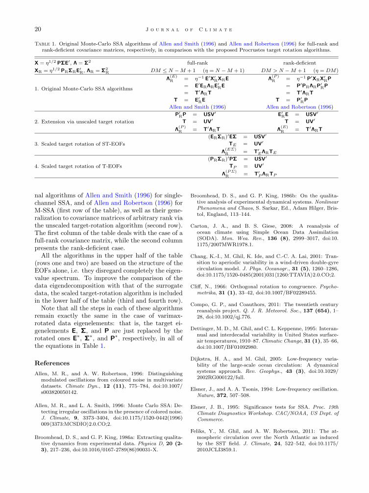
20 J o u r n a l o f C l i m a t e
Table 1. Original Monte-Carlo SSA algorithms of Allen and Smith (1996) and Allen and Robertson (1996) for full-rank andrank-deficient covariance matrices, respectively, in comparison with the proposed Procrustes target rotation algorithms.
X = η1/2 PΣE′, Λ = Σ2 full-rank rank-deficient
XR = η1/2 PRΣRE′R, ΛR = Σ2R DM ≤ N −M + 1 (η = N −M + 1) DM > N −M + 1 (η = DM)
1. Original Monte-Carlo SSA algorithms
Λ(E)R = η−1 E′X′RXRE
= E′ERΛRE′RE
= T′ΛRT
T = E′RE
Λ(P )R = η−1 P′XRX′RP
= P′PRΛRP′RP
= T′ΛRT
T = P′RP
Allen and Smith (1996) Allen and Robertson (1996)
2. Extension via unscaled target rotation
P′RP = USV′
T = UV′
Λ(P )R = T′ΛRT
E′RE = USV′
T = UV′
Λ(E)R = T′ΛRT
3. Scaled target rotation of ST-EOFs
(ERΣR)′EΣ = USV′
TE = UV′
Λ(EΣ)R = T′EΛRTE
4. Scaled target rotation of T-EOFs
(PRΣR)′PΣ = USV′
TP = UV′
Λ(PΣ)R = T′PΛRTP
nal algorithms of Allen and Smith (1996) for single-channel SSA, and of Allen and Robertson (1996) forM-SSA (first row of the table), as well as their gene-ralization to covariance matrices of arbitrary rank viathe unscaled target-rotation algorithm (second row).The first column of the table deals with the case of afull-rank covariance matrix, while the second columnpresents the rank-deficient case.
All the algorithms in the upper half of the table(rows one and two) are based on the structure of theEOFs alone, i.e. they disregard completely the eigen-value spectrum. To improve the comparison of thedata eigendecomposition with that of the surrogatedata, the scaled target-rotation algorithm is includedin the lower half of the table (third and fourth row).
Note that all the steps in each of these algorithmsremain exactly the same in the case of varimax-rotated data eigenelements: that is, the target ei-genelements E, Σ, and P are just replaced by therotated ones E∗, Σ∗, and P∗, respectively, in all ofthe equations in Table 1.
References
Allen, M. R., and A. W. Robertson, 1996: Distinguishingmodulated oscillations from coloured noise in multivariatedatasets. Climate Dyn., 12 (11), 775–784, doi:10.1007/s003820050142.
Allen, M. R., and L. A. Smith, 1996: Monte Carlo SSA: De-tecting irregular oscillations in the presence of colored noise.J. Climate, 9, 3373–3404, doi:10.1175/1520-0442(1996)009〈3373:MCSDIO〉2.0.CO;2.
Broomhead, D. S., and G. P. King, 1986a: Extracting qualita-tive dynamics from experimental data. Physica D, 20 (2-3), 217–236, doi:10.1016/0167-2789(86)90031-X.
Broomhead, D. S., and G. P. King, 1986b: On the qualita-tive analysis of experimental dynamical systems. NonlinearPhenomena and Chaos, S. Sarkar, Ed., Adam Hilger, Bris-tol, England, 113–144.
Carton, J. A., and B. S. Giese, 2008: A reanalysis ofocean climate using Simple Ocean Data Assimilation(SODA). Mon. Wea. Rev., 136 (8), 2999–3017, doi:10.1175/2007MWR1978.1.
Chang, K.-I., M. Ghil, K. Ide, and C.-C. A. Lai, 2001: Tran-sition to aperiodic variability in a wind-driven double-gyrecirculation model. J. Phys. Oceanogr., 31 (5), 1260–1286,doi:10.1175/1520-0485(2001)031〈1260:TTAVIA〉2.0.CO;2.
Cliff, N., 1966: Orthogonal rotation to congruence. Psycho-metrika, 31 (1), 33–42, doi:10.1007/BF02289455.
Compo, G. P., and Coauthors, 2011: The twentieth centuryreanalysis project. Q. J. R. Meteorol. Soc., 137 (654), 1–28, doi:10.1002/qj.776.
Dettinger, M. D., M. Ghil, and C. L. Keppenne, 1995: Interan-nual and interdecadal variability in United States surface-air temperatures, 1910–87. Climatic Change, 31 (1), 35–66,doi:10.1007/BF01092980.
Dijkstra, H. A., and M. Ghil, 2005: Low-frequency varia-bility of the large-scale ocean circulation: A dynamicalsystems approach. Rev. Geophys., 43 (3), doi:10.1029/2002RG000122/full.
Elsner, J., and A. A. Tsonis, 1994: Low-frequency oscillation.Nature, 372, 507–508.
Elsner, J. B., 1995: Significance tests for SSA. Proc. 19thClimate Diagnostics Workshop. CAC/NOAA, US Dept. ofCommerce.
Feliks, Y., M. Ghil, and A. W. Robertson, 2011: The at-mospheric circulation over the North Atlantic as inducedby the SST field. J. Climate, 24, 522–542, doi:10.1175/2010JCLI3859.1.

J o u r n a l o f C l i m a t e 21
Feliks, Y., A. Groth, A. W. Robertson, and M. Ghil, 2013:Oscillatory climate modes in the Indian Monsoon, NorthAtlantic and Tropical Pacific. J. Climate, 26, 9528–9544,doi:10.1175/JCLI-D-13-00105.1.
Fukunaga, K., 1990: Introduction to statistical pattern recog-nition. 2nd ed., Academic Press.
Gamiz-Fortis, S., D. Pozo-Vazquez, M. Esteban-Parra, andY. Castro-Dıez, 2002: Spectral characteristics and pre-dictability of the NAO assessed through singular spectralanalysis. J. Geophys. Res., 107 (D23), ACL–11, doi:10.1029/2001JD001436.
Ghil, M., Y. Feliks, and L. Sushama, 2002a: Baroclinic and ba-rotropic aspects of the wind-driven ocean circulation. Phy-sica D, 167 (1), 1–35.
Ghil, M., and R. Vautard, 1991: Interdecadal oscillations andthe warming trend in global temperature time series. Na-ture, 350 (6316), 324–327, doi:10.1038/350324a0.
Ghil, M., and Coauthors, 2002b: Advanced spectral methodsfor climatic time series. Rev. Geophys., 40 (1), 1–41, doi:10.1029/2000RG000092.
Giese, B. S., and S. Ray, 2011: El Nino variability in Sim-ple Ocean Data Assimilation (SODA), 1871–2008. Journalof Geophysical Research: Oceans (1978–2012), 116 (C2),doi:10.1029/2010JC006695.
Golyandina, N., V. Nekrutkin, and A. Zhigliavsky, 2001: Ana-lysis of time series structure: SSA and related techniques.Chapman & Hall/CRC.
Golyandina, N., and A. A. Zhigljavsky, 2013: SingularSpectrum Analysis for Time Series. Springer Berlin Hei-delberg.
Green, B., 1952: The orthogonal approximation of an obliquestructure in factor analysis. Psychometrika, 17 (4), 429–440, doi:10.1007/BF02288918.
Groth, A., and M. Ghil, 2011: Multivariate singular spectrumanalysis and the road to phase synchronization. Phys. Rev.E, 84, 036 206, doi:10.1103/PhysRevE.84.036206.
Holmstrom, L., and I. Launonen, 2013: Posterior singularspectrum analysis. Stat. Anal. Data Min., 6 (5), 387–402,doi:10.1002/sam.11195.
Hurley, J. R., and R. B. Cattell, 1962: The Procrustesprogram: Producing direct rotation to test a hypothe-sized factor structure. Behav. Sci., 7 (2), 258–262, doi:10.1002/bs.3830070216.
Jiang, S., F. Jin, and M. Ghil, 1995: Multiple equilibria, peri-odic, and aperiodic solutions in a wind-driven, double-gyre,shallow-water model. J. Phys. Oceanogr., 25 (5), 764–786.
Jolliffe, I. T., 2002: Principal Component Analysis. 2nd ed.,Springer.
Kaiser, H., 1958: The varimax criterion for analytic rotationin factor analysis. Psychometrika, 23 (3), 187–200, doi:10.1007/BF02289233.
Keppenne, C. L., and M. Ghil, 1993: Adaptive filtering andprediction of noisy multivariate signals: An application to
subannual variability in atmospheric angular momentum.Int. J. Bifurcat. Chaos, 3, 625–634.
Mane, R., 1981: On the dimension of the compact invariantsets of certain non-linear maps. Dynamical Systems andTurbulence, Lecture Notes in Mathematics, Vol. 898, Sprin-ger, Berlin, 230–242, doi:10.1007/BFb0091916.
Moron, V., R. Vautard, and M. Ghil, 1998: Trends, inter-decadal and interannual oscillations in global sea-surfacetemperatures. Climate Dyn., 14 (7), 545–569, doi:10.1007/s003820050241.
North, G. R., T. L. Bell, R. F. Cahalan, and F. J. Moeng, 1982:Sampling errors in the estimation of empirical orthogonalfunctions. Mon. Wea. Rev., 110 (7), 699–706, doi:10.1175/1520-0493(1982)110〈0699:SEITEO〉2.0.CO;2.
O’Lenic, E. A., and R. E. Livezey, 1988: Practical consi-derations in the use of rotated principal component ana-lysis (RPCA) in diagnostic studies of upper-air heightfields. Mon. Wea. Rev., 116 (8), 1682–1689, doi:10.1175/1520-0493(1988)116〈1682:PCITUO〉2.0.CO;2.
Palus, M., and D. Novotna, 2004: Enhanced Monte Carlosingular system analysis and detection of period 7.8 yearsoscillatory modes in the monthly NAO index and tempe-rature records. Nonlinear Processes Geophys., 11 (5/6),721–729, URL http://www.nonlin-processes-geophys.net/11/721/2004/.
Paunonen, S. V., 1997: On chance and factor congruence follo-wing orthogonal Procrustes rotation. Educ. Psychol. Meas.,57 (1), 33–59, doi:10.1177/0013164497057001003.
Plaut, G., and R. Vautard, 1994: Spells of low-frequency oscil-lations and weather regimes in the Northern Hemisphere. J.Atmos. Sci., 51 (2), 210–236, doi:10.1175/1520-0469(1994)051〈0210:SOLFOA〉2.0.CO;2.
Richman, M. B., 1986: Rotation of principal components. Int.J. Climatol., 6 (3), 293–335, doi:10.1002/joc.3370060305.
Robertson, A. W., 1996: Interdecadal variability over theNorth Pacific in a multi-century climate simulation. Cli-mate Dyn., 12 (4), 227–241, doi:10.1007/BF00219498.
Schonemann, P., 1966: A generalized solution of the ortho-gonal Procrustes problem. Psychometrika, 31, 1–10, doi:10.1007/BF02289451.
Speich, S., H. Dijkstra, and M. Ghil, 1995: Successive bifurca-tions in a shallow-water model applied to the wind-drivenocean circulation. Nonlinear Processes Geophys., 2, 241–268.
Takens, F., 1981: Detecting strange attractors in turbulence.Dynamical Systems and Turbulence, Lecture Notes in Mat-hematics, Vol. 898, Springer, Berlin, 366–381.
Vautard, R., and M. Ghil, 1989: Singular spectrum ana-lysis in nonlinear dynamics, with applications to paleo-climatic time series. Physica D, 35 (3), 395–424, doi:10.1016/0167-2789(89)90077-8.
Vautard, R., P. Yiou, and M. Ghil, 1992: Singular-spectrumanalysis: A toolkit for short, noisy chaotic signals. PhysicaD, 58 (1-4), 95–126, doi:10.1016/0167-2789(92)90103-T.


![Data-adaptive Harmonic Decomposition and Real-time ... · Key di erence from Multichannel Singular Spectrum Analysis (M-SSA) [Ghil et al. 2002, Rev. Geophys. ]: DAH is frequency-based,](https://img.pdfslide.us/doc/110x75/5f4ee38a479df52f0071702e/data-adaptive-harmonic-decomposition-and-real-time-key-di-erence-from-multichannel.jpg)


![The Sliding Singular Spectrum Analysis: a Data-Driven Non ... · INGULAR Spectrum Analysis (SSA) [1], [2] is a data-adaptive and non parametric method for time series de-composition](https://img.pdfslide.us/doc/110x75/600dab980db6c15d0116f7b7/the-sliding-singular-spectrum-analysis-a-data-driven-non-ingular-spectrum-analysis.jpg)