Monte Carlo Simulation of StochasticProcesses

Last update: January 10th, 2004.

In this section is presented the steps to perform the simulation of the main stochastic processesused in real options applications, that is the Geometric Brownian Motion, the Mean ReversionProcess and the combined process of Mean-Reversion with Jumps.

For all cases I present both simulations the risk-neutral and the real one. Risk-neutralsimulations are used for derivatives pricing, whereas real simulations are used for value at risk,hedging and, for real options applications, is useful for example to find the probability ofexercise the option and the expected time to wait before the option exercise (see the new Timingspreadsheet).See the FAQ 4 for a discussion of risk-neutral versus real simulations.

This section includes the topics:

Monte Carlo Simulation of Geometric Brownian Motion

Monte Carlo Simulation of Mean Reversion (Model 1)

Complement: Discretization Accuracy of the Mean-Reversion Stochastic Process. NEW!. . . Download an Excel spreadsheet that simulates this mean-reversion model and discusses thediscretization accuracy. NEW!

Monte Carlo Simulation of Mean Reversion (Model 2).A More Practical Approach to Mean Reversion Model 2. NEW! November 2003 insertion .

Monte Carlo Simulation of Mean Reversion with Jumps. . . Download a spreadsheet simulating the mean-reversion + jumps sample paths. NEW!

Monte Carlo Simulation of Geometric Brownian Motion

Consider that the price P of a commodity follows a Geometric Brownian Motion, which is givenby the following stochastic equation:

dP = αααα P dt + σσσσ P dz

Where dz = Wiener increment = ε dt0.5, ε is the standard normal distribution; α is the drift (orcapital gain rate); and σ is the volatility of P.

By using the equation of total investment return µ = α + δµ = α + δµ = α + δµ = α + δ, where µ is also the risk-adjusted

discount rate for P; and δ is the dividend yield (or convenience yield in case of commodities).We can rewrite the stochastic equation as:

dP = (µ − δ)(µ − δ)(µ − δ)(µ − δ) P dt + σσσσ P dz

For the risk-neutral version of this equation, just replace the risk-adjusted discount rate µ by therisk-free interest rate r to obtain the risk-neutral stochastic equation:

dP = ((((r − δ) − δ) − δ) − δ) P dt + σσσσ P dz

Using a logarithm transformation and applying the Itô's Lemma, we can reach the equations forthe prices simulation in both formats, real and risk-neutral.For more technical details, see the page on Geometric Brownian Motion, from the StochasticProcesses section.

The real simulation of a GBM uses the real drift αααα. The price Pt at the future instant t is givenby:

The simulation of the real prices using the above equation is done by sampling the standardNormal distribution N(0, 1) and obtaining the correspondent values for Pt. These values of P canbe used to calculate the (real) values of the project V by means of some equation V(P) orcombined even with other uncertain variables in order to obtain the real value of V.Remember, with the real drift simulation of the underlying asset (P), the required discount rate isthe risk-adjusted one µ. Real simulations are used mainly for the calculus of the probability ofoption exercise and for the expected time of option exercise (given conditional to have occur atleast one exercise in the simulation), see the new Timing spreadsheet. In financial applications,the real simulation is used for VaR (value at Risk) estimation.However, for derivatives in general is required other type of simulation, the risk-neutral one,because the risk-adjusted discount rate for the derivative F(P) in general is not the same µ usedfor P.

The risk-neutral simulation of a GBM uses the risk-neutral drift α’ = r − δ . The price at t is:

The simulation of the risk-neutral prices using the above equation is performed by sampling thestandard Normal distribution N(0, 1) and obtaining the correspondent values for Pt. The risk-neutral simulation is used mainly for the derivatives valuation in complete markets. Forincomplete markets, is possible use either the risk-neutral one (but need to select a martingalemeasure from several or to estimate the risk-premium in this market) or the real simulation onewith an exogenous risk-adjusted discount rate (dynamic programming), see FAQ 5.However, for both the estimation of the probability of option exercise and the expected time ofoption exercise, the correct is the real simulation and not the risk-neutral one.

One important feature of the above discrete-time equations is that the discretization from the

continuous-time model is exact. In other words, you don't need to use small time increments ∆tin order to get a good approximation. You can use any ∆t that the simulation equation is valid(check out this affirmative by evaluating an European call option with time to maturity of oneyear, for example, by risk-neutral simulation of the underlying asset only at the expiration, andconferring with the exact Black-Scholes formula result).

Monte Carlo Simulation of Mean Reversion (Model 1)

Initially consider the following Arithmetic Ornstein-Uhlenbeck process for a stochastic variablex(t):

This means that there is a reversion force over the variable x pulling towards an equilibriumlevel , like a spring force.The velocity of the reversion process is given by the parameter ηηηη.

This stochastic differential equation is explicitly solvable (see Kloeden & Platen, 1992, topic 4.4,eq.4.2) and has the following solution in terms of stochastic integral (Itô's integral):

The variable x(T) has Normal distribution with the following expressions for the mean andvariance (see for example Dixit & Pindyck, 1994, chapter 3):

In the expected value equation note that the mean is just a weighted average between the initiallevel x(0) and the long-run level (the weights sum one and are functions of the time and thereversion speed).The variance increases with the time, but also converges to σ2/(2η) as the time goes to infinite.See the textbook of Oksendal ("Stochastic Differential Equations - An Introduction withApplications") for details on Itô's stochastic integration, and the exercise (with answer) for themean-reversion process.There is the following relation between the mean-reversion speed (η) and the half-life (H) of theprocess: H = ln(2)/ηηηη (click here for the proof). Half-life is the time that is expected time for thestochastic variable x to reach the half of way toward the equilibrium level .

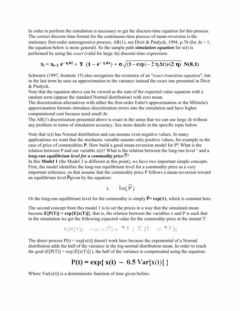
In order to perform the simulation is necessary to get the discrete-time equation for this process.The correct discrete-time format for the continuous-time process of mean-reversion is thestationary first-order autoregressive process, AR(1), see Dixit & Pindyck, 1994, p.76 (for ∆t = 1,the equation below is more general). So the sample path simulation equation for x(t) isperformed by using the exact (valid for large ∆t) discrete-time expression:

Schwartz (1997, footnote 15) also recognizes the existence of an "exact transition equation", butin the last term he uses an approximation to the variance instead the exact one presented in Dixit& Pindyck.Note that the equation above can be viewed as the sum of the expected value equation with arandom term (appear the standard Normal distribution) with zero mean.The discretization alternatives with either the first-order Euler's approximation or the Milstein'sapproximation formats introduce discretization errors into the simulation and have highercomputational cost because need small ∆t.The AR(1) discretization presented above is exact in the sense that we can use large ∆t withoutany problem in terms of simulation accuracy. See more details in the specific topic below.

Note that x(t) has Normal distribution and can assume even negative values. In manyapplications we want that the stochastic variable assume only positive values, for example in thecase of price of commodities P. How build a good mean-reversion model for P? What is therelation between P and our variable x(t)? What is the relation between the long-run level and along-run equilibrium level for a commodity price ?In this Model 1 (the Model 2 is different at this point), we have two important simple concepts.First, the model identifies the long-run equilibrium level for a commodity price as a veryimportant reference, so that assume that the commodity price P follows a mean-reversion towardan equilibrium level given by the equation:

Or the long-run equilibrium level for the commodity is simply = exp( ), which is constant here.

The second concept from this model 1 is to set the prices in a way that the simulated meanbecome E[P(T)] = exp{E[x(T)]}, that is, the relation between the variables x and P is such thatin the simulation we get the following expected value for the commodity price at the instant T:

The direct process P(t) = exp[x(t)] doesn't work here because the exponential of a Normaldistribution adds the half of the variance in the log-normal distribution mean. In order to reachthe goal (E[P(T)] = exp{E[x(T)]}), the half of the variance is compensated using the equation:

Where Var[x(t)] is a deterministic function of time given before.

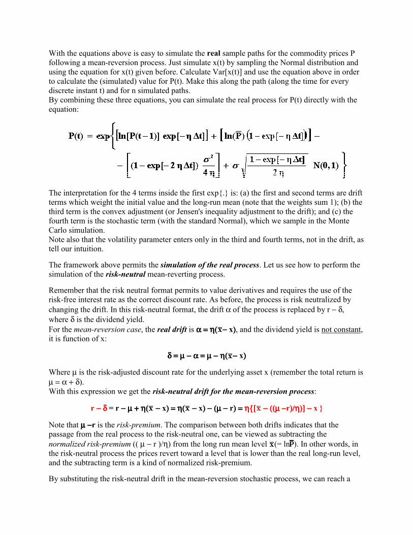
With the equations above is easy to simulate the real sample paths for the commodity prices Pfollowing a mean-reversion process. Just simulate x(t) by sampling the Normal distribution andusing the equation for x(t) given before. Calculate Var[x(t)] and use the equation above in orderto calculate the (simulated) value for P(t). Make this along the path (along the time for everydiscrete instant t) and for n simulated paths.By combining these three equations, you can simulate the real process for P(t) directly with theequation:

The interpretation for the 4 terms inside the first exp{.} is: (a) the first and second terms are driftterms which weight the initial value and the long-run mean (note that the weights sum 1); (b) thethird term is the convex adjustment (or Jensen's inequality adjustment to the drift); and (c) thefourth term is the stochastic term (with the standard Normal), which we sample in the MonteCarlo simulation.Note also that the volatility parameter enters only in the third and fourth terms, not in the drift, astell our intuition.

The framework above permits the simulation of the real process. Let us see how to perform thesimulation of the risk-neutral mean-reverting process.

Remember that the risk neutral format permits to value derivatives and requires the use of therisk-free interest rate as the correct discount rate. As before, the process is risk neutralized bychanging the drift. In this risk-neutral format, the drift α of the process is replaced by r − δ,where δ is the dividend yield.For the mean-reversion case, the real drift is α = η(α = η(α = η(α = η( −−−− x)))), and the dividend yield is not constant,it is function of x:

δ = µ − α = µ − η(δ = µ − α = µ − η(δ = µ − α = µ − η(δ = µ − α = µ − η( −−−− x))))

Where µ is the risk-adjusted discount rate for the underlying asset x (remember the total return isµ = α + δ).With this expression we get the risk-neutral drift for the mean-reversion process:

r − δ− δ− δ− δ = r − µ + η(− µ + η(− µ + η(− µ + η( −−−− x) = η() = η() = η() = η( −−−− x) − (µ −) − (µ −) − (µ −) − (µ − r) =) =) =) = η{[η{[η{[η{[ − ((µ − − ((µ − − ((µ − − ((µ −r)/η)] −)/η)] −)/η)] −)/η)] − x }

Note that µ −µ −µ −µ −r is the risk-premium. The comparison between both drifts indicates that thepassage from the real process to the risk-neutral one, can be viewed as subtracting thenormalized risk-premium (( µ − r )/η) from the long run mean level (= ln ). In other words, inthe risk-neutral process the prices revert toward a level that is lower than the real long-run level,and the subtracting term is a kind of normalized risk-premium.

By substituting the risk-neutral drift in the mean-reversion stochastic process, we can reach a

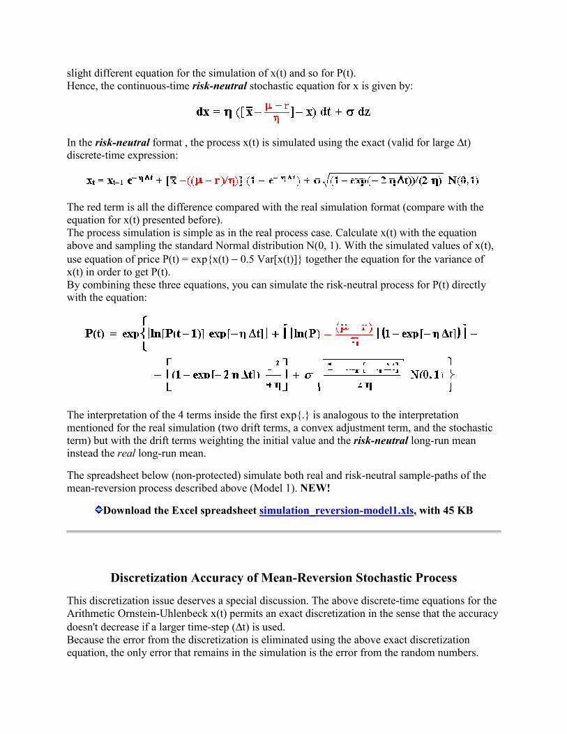
slight different equation for the simulation of x(t) and so for P(t).Hence, the continuous-time risk-neutral stochastic equation for x is given by:

In the risk-neutral format , the process x(t) is simulated using the exact (valid for large ∆t)discrete-time expression:

The red term is all the difference compared with the real simulation format (compare with theequation for x(t) presented before).The process simulation is simple as in the real process case. Calculate x(t) with the equationabove and sampling the standard Normal distribution N(0, 1). With the simulated values of x(t),use equation of price P(t) = exp{x(t) − 0.5 Var[x(t)]} together the equation for the variance ofx(t) in order to get P(t).By combining these three equations, you can simulate the risk-neutral process for P(t) directlywith the equation:

The interpretation of the 4 terms inside the first exp{.} is analogous to the interpretationmentioned for the real simulation (two drift terms, a convex adjustment term, and the stochasticterm) but with the drift terms weighting the initial value and the risk-neutral long-run meaninstead the real long-run mean.

The spreadsheet below (non-protected) simulate both real and risk-neutral sample-paths of themean-reversion process described above (Model 1). NEW!

Download the Excel spreadsheet simulation_reversion-model1.xls, with 45 KB

Discretization Accuracy of Mean-Reversion Stochastic Process

This discretization issue deserves a special discussion. The above discrete-time equations for theArithmetic Ornstein-Uhlenbeck x(t) permits an exact discretization in the sense that the accuracydoesn't decrease if a larger time-step (∆t) is used.Because the error from the discretization is eliminated using the above exact discretizationequation, the only error that remains in the simulation is the error from the random numbers.

This topic discusses the motivation to use a better discretization when available, includingreference to a list of stochastic processes that permit an exact discretization. This topic alsopresents an Excel spreadsheet - available to download, that shows in practice the superiority ofthe exact discretization over the popular Euler's approximation.

The use of large ∆t is much more important in real options (long-term options) than in financialoptions - although it is useful also for European financial options. Perhaps this explain that mostbooks ignore the exact simulation equation for mean-reversion, insisting to teach only Euler andMilstein approximations even when exact solutions are available.One exception is the textbook of Kloeden & Platen (1992) that in the topic 4.4 list "Someexplicitly solvable SDEs". The Arithmetic Ornstein-Uhlenbeck is their equation 4.2 (for thegeometric Brownian motion, see eq. 4.6 from this textbook). Kloeden & Platen use the explicitlysolvable SDEs (solution doesn't depend on small ∆t) to check the accuracy of numerical methodsthat depends on ∆t (like Euler approximations). See pp.308-310 for the geometric Brownianexample.

The spreadsheet below simulate this mean-reversion stochastic process, Model 1, using threedifferent discretization methods in order to show that the exact method presented above is themost accurate one.The spreadsheet also plots the histogram chart (the theoretical is a log-normal distribution) forthe simulated values of the mean-reverting commodity price at a specified time T and for theother specified parameters set by the user.

Download the Excel spreadsheet reversion-simulation_accuracy-vba.xls, with 372 KB

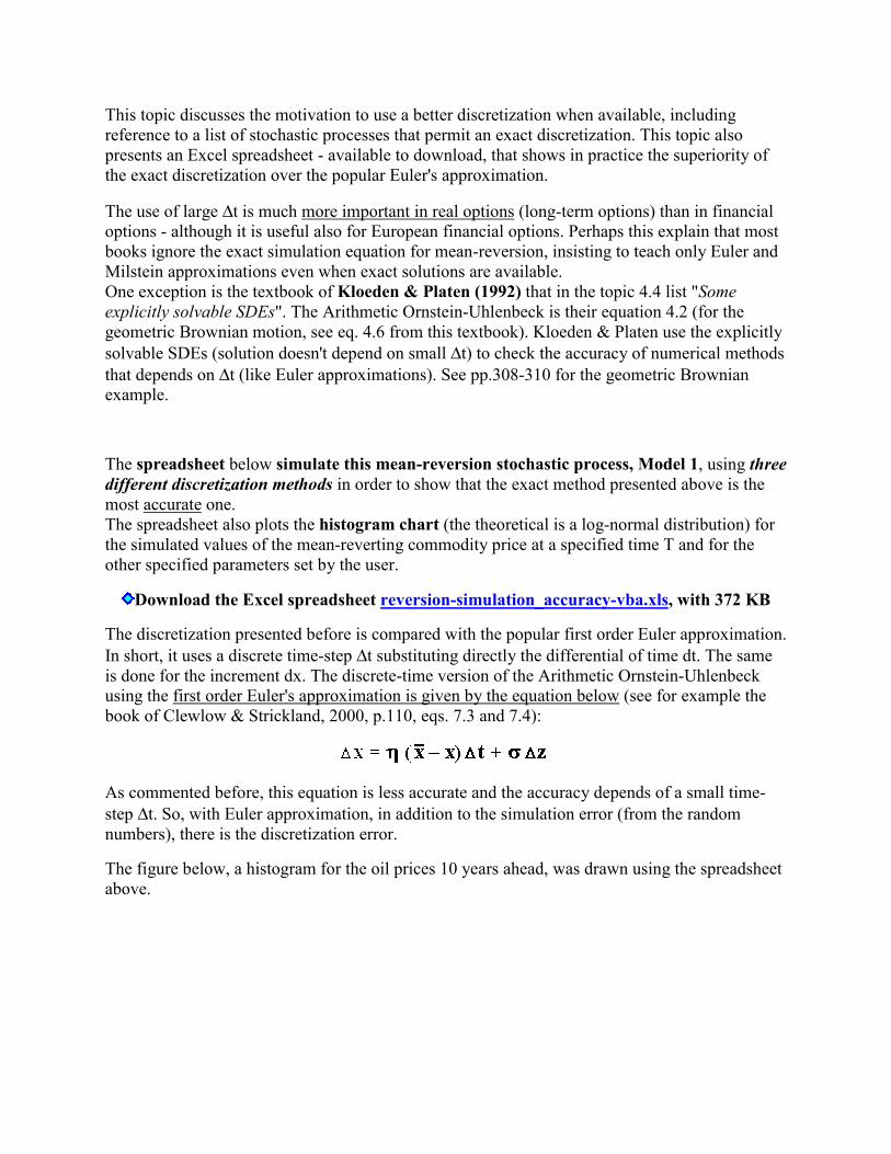
The discretization presented before is compared with the popular first order Euler approximation.In short, it uses a discrete time-step ∆t substituting directly the differential of time dt. The sameis done for the increment dx. The discrete-time version of the Arithmetic Ornstein-Uhlenbeckusing the first order Euler's approximation is given by the equation below (see for example thebook of Clewlow & Strickland, 2000, p.110, eqs. 7.3 and 7.4):

As commented before, this equation is less accurate and the accuracy depends of a small time-step ∆t. So, with Euler approximation, in addition to the simulation error (from the randomnumbers), there is the discretization error.

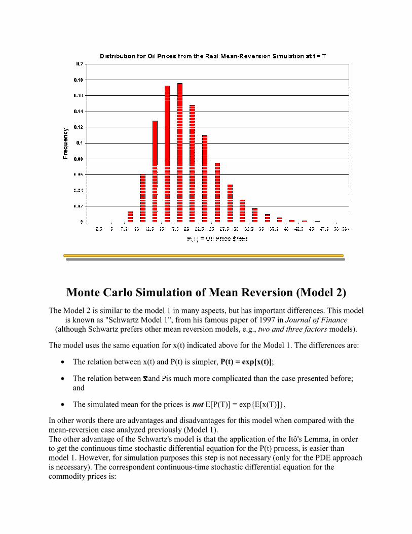
The figure below, a histogram for the oil prices 10 years ahead, was drawn using the spreadsheetabove.

Monte Carlo Simulation of Mean Reversion (Model 2)

The Model 2 is similar to the model 1 in many aspects, but has important differences. This modelis known as "Schwartz Model 1", from his famous paper of 1997 in Journal of Finance

(although Schwartz prefers other mean reversion models, e.g., two and three factors models).

The model uses the same equation for x(t) indicated above for the Model 1. The differences are:

• The relation between x(t) and P(t) is simpler, P(t) = exp[x(t)];

• The relation between and is much more complicated than the case presented before;and

• The simulated mean for the prices is not E[P(T)] = exp{E[x(T)]}.

In other words there are advantages and disadvantages for this model when compared with themean-reversion case analyzed previously (Model 1).The other advantage of the Schwartz's model is that the application of the Itô's Lemma, in orderto get the continuous time stochastic differential equation for the P(t) process, is easier thanmodel 1. However, for simulation purposes this step is not necessary (only for the PDE approachis necessary). The correspondent continuous-time stochastic differential equation for thecommodity prices is:

dP = ηηηη( ln −−−− lnP) P dt + σσσσ P dz

This is the Schwartz's eq.1 with other notation. The relation between and is given by theequation (see the eq. 3 in Schwartz, 1997):

= ln − − − − (σσσσ2/(2ηηηη))

Hence the expected long-run equilibrium price (real process) depends on both the volatility andthe reversion speed.The real simulation of this model is given by the following equation that again uses an exactdiscretization that allows large ∆t (correcting an old version of this website):

Pt = exp{ [ln(Pt - 1) (exp(−η−η−η−η ∆∆∆∆t))] + [(ln −−−− (σσσσ2/(2ηηηη))) (1 −−−− exp(−η−η−η−η ∆∆∆∆t))] + [σσσσ (SQRT((1−−−−exp(−−−−2η ∆η ∆η ∆η ∆t))/(2ηηηη))) N(0,1)] }

Where the SQRT(.) is the square root operator. The simulation again is very simple, you get thesample paths of P(t) by sampling the Normal distribution. and using the equation above.The expected value for P(t) in the simulation is given by taking the expectations (including theconvexity adjustment) in the above equation:

E[Pt] = exp{ [ln(Pt - 1) (exp(−η−η−η−η ∆∆∆∆t))] + [(ln −−−− (σσσσ2/(2ηηηη)) (1 −−−− exp(−η−η−η−η ∆∆∆∆t))] + [(σσσσ2/(4ηηηη)) (1 −−−−exp(−−−−2ηηηη ∆∆∆∆t))] }

In the long-run (large t), the real simulation converge to the following expected long-run level:

F = E[P( )] = Expected Long-Run Futures Price = exp[ + + + + (σσσσ2/(4ηηηη))] = exp[ln − − − − (σσσσ2/(4ηηηη))]= exp[− σ− σ− σ− σ2/(4ηηηη)]

For the risk-neutral simulation, just subtract from (here = ln − σ2/[2η]) the normalized risk-premium (µ − r )/η, that is, the risk-neutral equation is given by:

Pt = exp{ [ln(Pt - 1) (exp(−η−η−η−η ∆∆∆∆t))] + [(ln −−−− (σσσσ2/(2ηηηη) −−−− ((µ −µ −µ −µ − r )/ηηηη)) (1 −−−− exp(−η−η−η−η ∆∆∆∆t))] + [σσσσ(SQRT((1−−−− exp(−−−−2η ∆η ∆η ∆η ∆t))/(2ηηηη))) N(0,1)] }

If you take expectation of the above equation you get the Schwartz's eq.7 for the expected valueof the futures prices in the risk-neutral format (or "under martingale measure", as Schwartzprefers) because the random term (the last one inside the exponential operator) has zero mean(from standard Normal distribution) and considering the convexity adjustment.

On similar way, the expected commodity price in the risk-neutral simulation converges in thelong-run (very large t) to the following equation (compare with Schwartz eq. 38):

Expected Long-Run Risk-Neutral Futures Price = exp[ −−−− ((µ −µ −µ −µ − r )/ηηηη) + + + + (σσσσ2/(4ηηηη))]

See more about the differences between risk-neutral process and real drift process for the mean-reversion case in the FAQ13.

However, I prefer the model 1 than model 2 because is more simple to see where the simulation

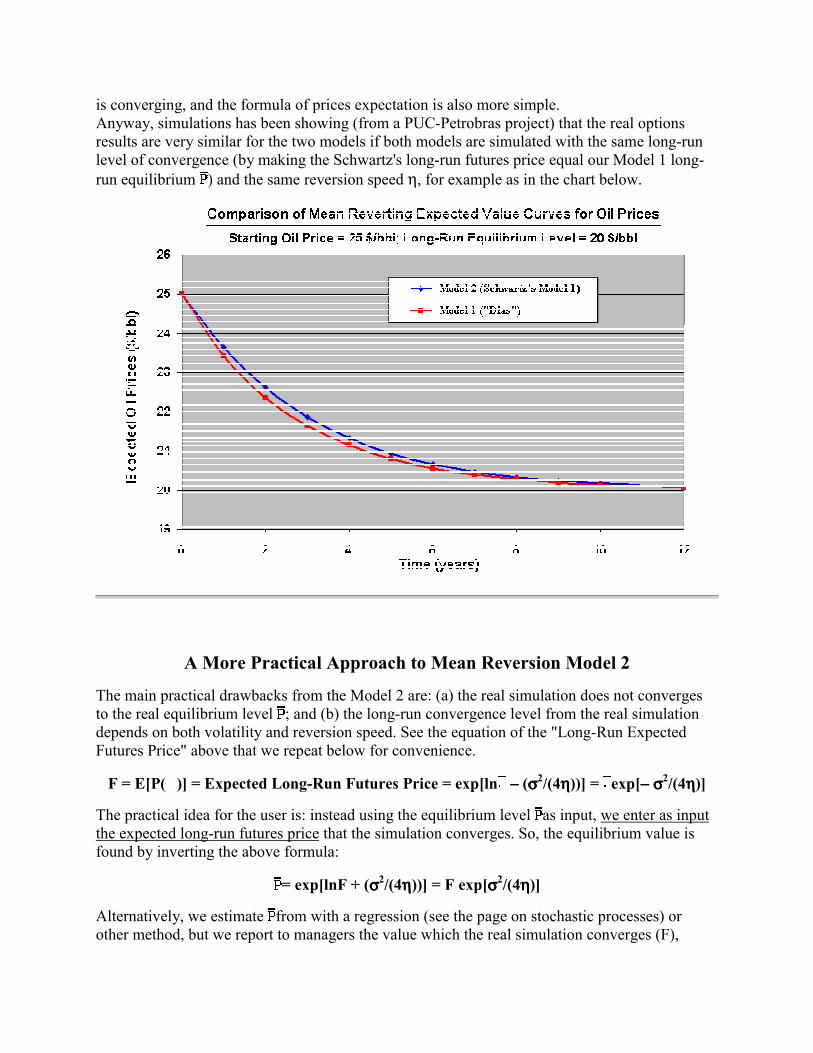
is converging, and the formula of prices expectation is also more simple.Anyway, simulations has been showing (from a PUC-Petrobras project) that the real optionsresults are very similar for the two models if both models are simulated with the same long-runlevel of convergence (by making the Schwartz's long-run futures price equal our Model 1 long-run equilibrium ) and the same reversion speed η, for example as in the chart below.

A More Practical Approach to Mean Reversion Model 2

The main practical drawbacks from the Model 2 are: (a) the real simulation does not convergesto the real equilibrium level ; and (b) the long-run convergence level from the real simulationdepends on both volatility and reversion speed. See the equation of the "Long-Run ExpectedFutures Price" above that we repeat below for convenience.

F = E[P( )] = Expected Long-Run Futures Price = exp[ln − − − − (σσσσ2/(4ηηηη))] = exp[− σ− σ− σ− σ2/(4ηηηη)]

The practical idea for the user is: instead using the equilibrium level as input, we enter as inputthe expected long-run futures price that the simulation converges. So, the equilibrium value isfound by inverting the above formula:

= exp[lnF + (σσσσ2/(4ηηηη))] = F exp[σσσσ2/(4ηηηη)]

Alternatively, we estimate from with a regression (see the page on stochastic processes) orother method, but we report to managers the value which the real simulation converges (F),

which is much more relevant in practice than .

In this way, the simulation equation for the real prices process is given by:

Pt = exp{ [ln(Pt - 1) (exp(−η−η−η−η ∆∆∆∆t))] + [(ln F −−−− (σσσσ2/(4ηηηη))) (1 −−−− exp(−η−η−η−η ∆∆∆∆t))] + [σσσσ (SQRT((1−−−−exp(−−−−2η ∆η ∆η ∆η ∆t))/(2ηηηη))) N(0,1)] }

Where the input F has the managerial meaning of average long-run level that the simulationconverges.

For the risk-neutral simulation, the equation using F as input is obtained easily: just subtract fromln F the normalized risk-premium in a similar way done before. This is left as exercise for thereader.

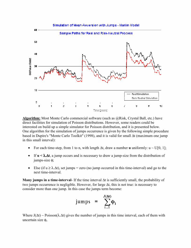
Monte Carlo Simulation of Mean Reversion with Jumps

This model, which I call Marlim Model (reference to Marlim, the top producer oilfield inBrazil), uses the first mean-reversion model presented before, but with the addition of randomjumps - modeled with a Poisson process. In addition, jumps are of random size. The jumpprocess dq is assumed to be independent of the continuous stochastic increment dz.Initially consider the following Arithmetic Ornstein-Uhlenbeck process with discrete jumps(modeled as a Poisson process) for a stochastic variable x(t):

This means that there is a reversion force over the variable x pulling towards an equilibrium level, like a spring force. The velocity of the reversion process is given by the parameter η. Jumps

are represented by the term dq, which most of time is zero and sometimes occur jumps ofuncertain size φφφφ and with arrival rate λλλλ.

dq = 0 with probability 1 − λ− λ− λ− λ dt

dq = φφφφ with probability λλλλ dt

The jump process dq is assumed independent of dz, the Wiener increment from the continuousprocess. That is, the Poisson process is independent of the mean-reverting process.The uncertain size of the jumps are modeled with the probability distribution φ. In the classicpaper of Merton (1976) of a jump-diffusion process, the jump-size distribution is assumed log-normal (so that the jumps occur in only one direction).

Here is allowed the possibility of both jumps-up and jumps-down, given that a jump occurred.Things are easier if we assume that there is the same probability of jump-up and jump-down, that

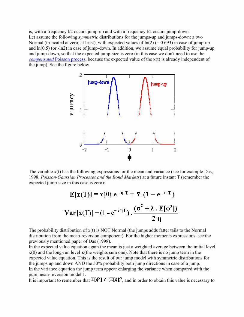
is, with a frequency l/2 occurs jump-up and with a frequency l/2 occurs jump-down.Let assume the following symmetric distributions for the jumps-up and jumps-down: a twoNormal (truncated at zero, at least), with expected values of ln(2) (= 0.693) in case of jump-upand ln(0.5) (or -ln2) in case of jump-down. In addition, we assume equal probability for jump-upand jump-down, so that the expected jump-size is zero (in this case we don't need to use thecompensated Poisson process, because the expected value of the x(t) is already independent ofthe jump). See the figure below.

The variable x(t) has the following expressions for the mean and variance (see for example Das,1998, Poisson-Gaussian Processes and the Bond Markets) at a future instant T (remember theexpected jump-size in this case is zero):

The probability distribution of x(t) is NOT Normal (the jumps adds fatter tails to the Normaldistribution from the mean-reversion component). For the higher moments expressions, see thepreviously mentioned paper of Das (1998).In the expected value equation again the mean is just a weighted average between the initial levelx(0) and the long-run level (the weights sum one). Note that there is no jump term in theexpected value equation. This is the result of our jump model with symmetric distributions forthe jumps up and down AND the 50% probability both jump directions in case of a jump.In the variance equation the jump term appear enlarging the variance when compared with thepure mean-reversion model 1.It is important to remember that , and in order to obtain this value is necessary to

estimate the integral:

Where f(φ) is the probability density function (in the present case the two Normal densities).This integral depends of the distribution φ but not of the jump arrival parameter λ (so that inpractice you can evaluate once the integral, if the jump size distribution is fixed).

The stochastic process for the commodity price P(t) is chosen so that the commodity prices arefunction of x(t) described by the first equation of this item.First let us to set the following relation between the long run process mean and the long-runequilibrium price of the commodity :

The idea is to set the prices in a way that the mean become E[P(T)] = eE[x(T)], that is, the relationbetween the variable x and P is such that in the simulation we get the following expected valuefor the commodity price at the instant T:

The direct process P(t) = ex(t) doesn't work here because the exponential of a normal distributionadds the half of the variance in the log-normal distribution mean. In order to reach the goal(E[P(T)] = eE[x(T)]), the half of the variance is compensated using the equation:

Where Var[x(t)] is a deterministic function of time, including the jumps contribution, givenbefore in this topic. In the literature (for example Fu et al., 2001), the half-variances of both thecontinuous process and jump process are subtracted in the simulation equation, but separately.

In the risk-neutral format , the process x(t) is simulated using the discrete-time expression withan appropriate time-step ∆t:

Where µ is the risk-adjusted discount rate for the underlying asset P. The red term ( µ - r )/η isthe normalized risk-premium subtracting the long run mean level (= ln( )).The simulation process is simple. Calculate x(t) with the equation above, sampling both thestandard Normal distribution N(0, 1) and the possibility of jump: Poisson process with parameterλup and λdown for jumps-up and jumps-down, respectively.Most of time the Poisson sampling points no jumps (dq = 0), but in case of jumps, we need tosampling the Normal distributions either for jumps-up or jumps-down.Now, with the simulated values of x(t), the simulation of P(t) is easy. Use equation of price P(t)= exp{x(t) − 0.5 Var[x(t)]} together the equation for the variance of x(t) in order to get P(t).

The term "jumps" in the equation above adds variance to the x(T) distribution. In case of adeterministic mean-reversion (σ = 0) with stochastic jumps, the jumps effect looks significative.The jumps effect on the variance of x(T) that most of time obeys a deterministic mean-revertingprocess is:

This variance initially grows but stabilizes for very long time T, due to the effect of the mean-reversion force. It is not difficult to see in the above equation that when, in addition to the σ = 0,the reversion speed η tends to zero (no mean-reversion) the pure jumps process with randomjump-size given by the probability distribution φ, has the following variance (take the limit inthe last equation):

Var[x(T)pure jumps] = λλλλ E[φφφφ2] T

Without the mean-reverting force, the variance of jumps grows with the time so that it is notbounded as before.

What is the appropriate time-step ∆∆∆∆t? Although the discretization for the mean-reverting part ofthe equation of x(t) is exact (valid for very large ∆t), the presence of jumps together with thereversion creates some problems to use large ∆t. For geometric Brownian process combined withjumps there is no problem because the process drift doesn't depend on the current level of thestochastic variable (it is possible even to use Brownian bridge with independent simulations foreach process). The same is not true for mean-reversion process - the drift is function of thecurrent value of the stochastic variable. Hence, the combination of reversion with jumps deservesmore caution.For the case with jumps combined with mean-reversion, I recommend to use a relatively small∆t, but larger than the required by Euler and Milstein approximations to reach a similar accuracy,in most cases.The idea is as follow. If the time interval ∆t is sufficiently small, the probability of two jumpsoccurrence is negligible because (λ.∆t)2 is much lower than (λ.∆t). So in this case we canconsider only one jump in each time interval.In order to illustrate the problem, imagine for example a ∆t = 1 year and λ = 1/year. Theprobability of occurrence of two jumps in one year is given by P[N(t) = n] = (1/n!) (λ t)n e− λ t =18.4% (make n = 2; λ = 1; t = 1), which is not negligible. If we consider both jumps at the endingof the year, the mean-reversion will not act through the year, reducing the jumps chocks effect atthe ending of the year. A very different result will occur if one jump is considered at thebeginning of the year (so the reversion will exercise a strong force along the year, and the otherone at the ending of the year.However, in the oil price process we are interested in rare large jumps only and we can usesmaller time-steps. Assume λ = 0.25 per annum (is expected only one jump each 4 years). Byusing a ∆t = 1 month (= 0.08 year), the probability of two jumps in this period (one month) isonly 0.02%, which is negligible (the probability of one jump is > 2% and is not negligible). Inpractice this means that we can assume only one jump using a smaller ∆t (as in this case).

Even for the case with jumps associated with the mean-reversion, is preferable to use the abovediscretization for x(t) than approximations for the mean-reverting part using Euler or Milsteinapproximations. The Euler or Milstein approximations require very small ∆t even without jumps.With jumps, a ∆t of one month in the above example means a larger error than using the exactdiscretization used for the mean-reverting part.

For the real process simulation (instead the risk-neutral one), use the same equation for x(t) , butwithout the normalized risk-premium ( µ - r )/η) subtracting the long run mean level (= ln( )),that is the real simulation for x(t) is given by:

The Excel spreadsheet available to download below, shows the real and risk-neutral sample-paths from a simulation of the mean-reversion with jumps, named Marlim model (press F9 toget new sample paths in the chart):

Download the Excel spreadsheet simulation-reversion-jumps-marlim-real_x_rn.xls, with235 KB

In the spreadsheet, were used a fixed jump-sizes for both jump-up and jump-down. However, itis easy to set probability distributions for the jumps-size. The formulas used in the spreadsheetare the ones presented above.

The chart below presents an example of sample paths simulation for both the real and the risk-neutral simulation of a mean-reversion with jumps, from the spreadsheet.In this example the Marlim model considered λ = 0.25 (is expected one jump each 4 years), withequal probability to be jump-up or jump-down; reversion with half-life of two years towards anequilibrium level of 20 $/bbl; volatility of 20%, etc (see the spreadsheet available before fordetails).

Algorithm: Most Monte Carlo commercial software (such as @Risk, Crystal Ball, etc.) havedirect facilities for simulation of Poisson distributions. However, some readers could beinterested on build up a simple simulator for Poisson distribution, and it is presented below.One algorithm for the simulation of jumps occurrence is given by the following simple procedurebased in Dupire's "Monte Carlo Toolkit" (1998), and it is valid for small ∆t (maximum one jumpin this small interval):

• For each time-step, from 1 to n, with length ∆t, draw a number u uniformly: u ~ U[0, 1];

• If u < λλλλ.∆∆∆∆t, a jump occurs and is necessary to draw a jump-size from the distribution ofjumps-size φ;

• Else (if u ≥ λ.∆t), set jumps = zero (no jump occurred in this time-interval) and go to thenext time-interval.

Many jumps in a time-interval- If the time interval ∆t is sufficiently small, the probability oftwo jumps occurrence is negligible. However, for large ∆t, this is not true: is necessary toconsider more than one jump. In this case the jumps term become:

Where J(∆t) ~ Poisson(λ.∆t) gives the number of jumps in this time interval, each of them withuncertain size φi.

In case of no jumps, in the equation above jumps = 0.In practical terms, make jumps = jumps-up + jumps-down, so we get two summations, one forjumps-up and another for jumps-down, each with arrival rate of λ/2 (if jump-up and jump-downhave 50% chances each in case of one jump) and with distributions φup and φdown, respectivelyinside the summations. However, again I recommend a small ∆t so that the probability of morethan one jump is negligible.

In order to consider more than one jump in each time-interval, it is necessary a more generalalgorithm for Poisson processes. This algorithm is generally based in the relationship betweenthe Poisson(λ) distribution and the exponential distribution, expo(1/λ), is given in the textbookof Law & Kelton (2000, p.478).

Back to Real Options with Monte Carlo Simulation Webpage

Back to Contents (The Main Page)