Monte Carlo Analysis A Technique for Combining Distributions

Monte Carlo Analysis

A Technique for Combining Distributions

FIN 591: Financial Modeling, Spring 2004

2

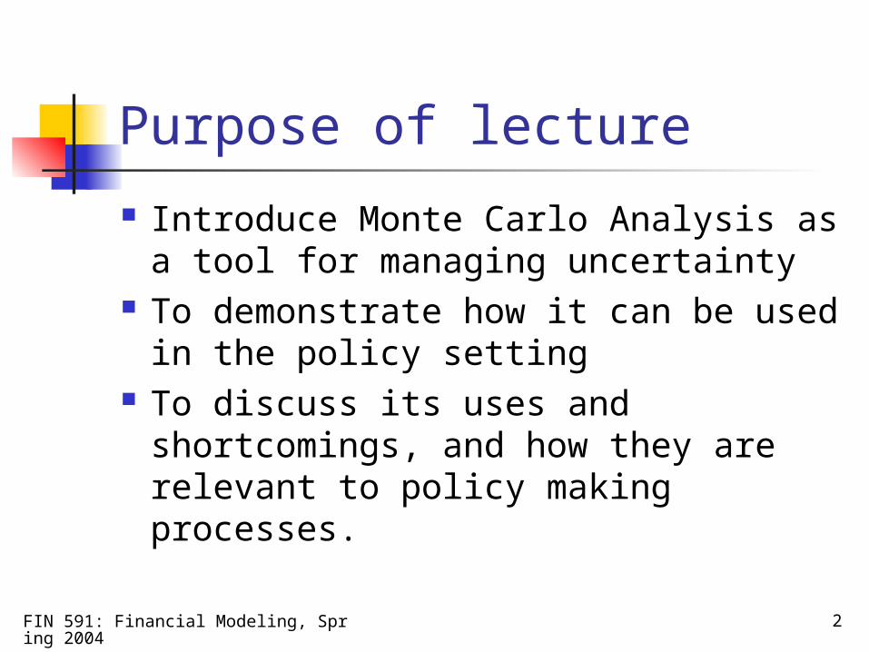
Purpose of lecture

Introduce Monte Carlo Analysis as a tool for managing uncertainty

To demonstrate how it can be used in the policy setting

To discuss its uses and shortcomings, and how they are relevant to policy making processes.


3

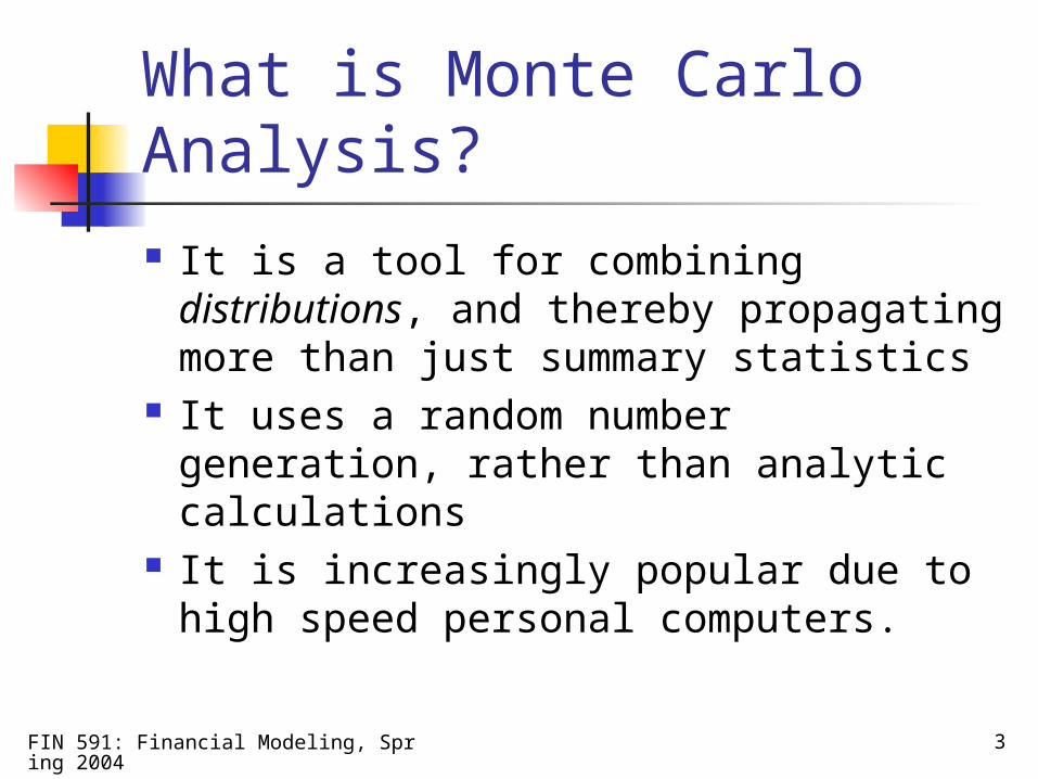
What is Monte Carlo Analysis?

It is a tool for combining distributions, and thereby propagating more than just summary statistics

It uses a random number generation, rather than analytic calculations

It is increasingly popular due to high speed personal computers.


4

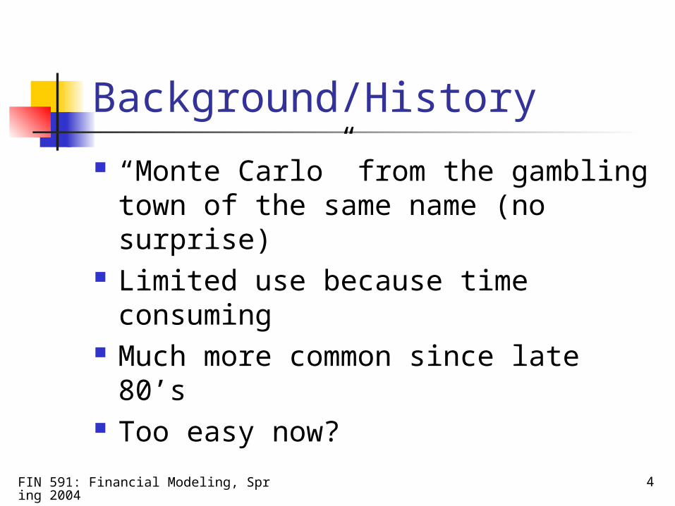
Background/History

“Monte Carlo” from the gambling town of the same name (no surprise)

Limited use because time consuming

Much more common since late 80’s Too easy now?


5

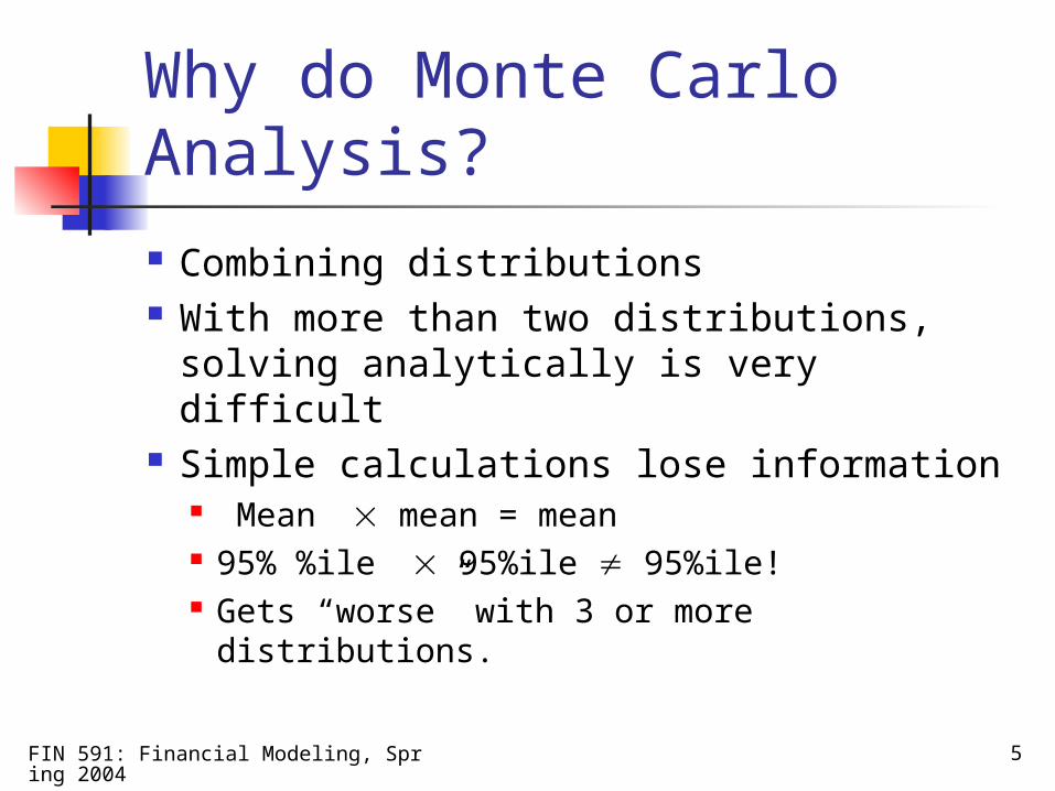
Why do Monte Carlo Analysis?

Combining distributions With more than two distributions,

solving analytically is very difficult Simple calculations lose information

Mean mean = mean 95% %ile 95%ile 95%ile! Gets “worse” with 3 or more

distributions.


6

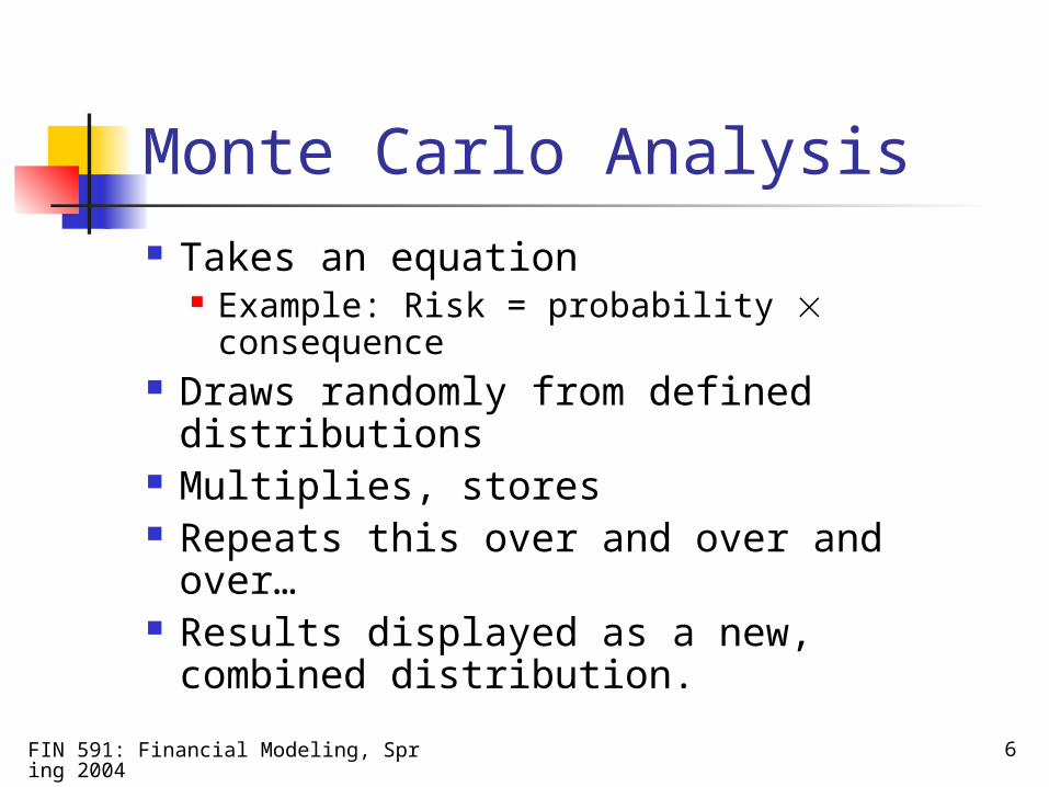
Monte Carlo Analysis Takes an equation

Example: Risk = probability consequence

Draws randomly from defined distributions

Multiplies, stores Repeats this over and over and over… Results displayed as a new, combined

distribution.


7

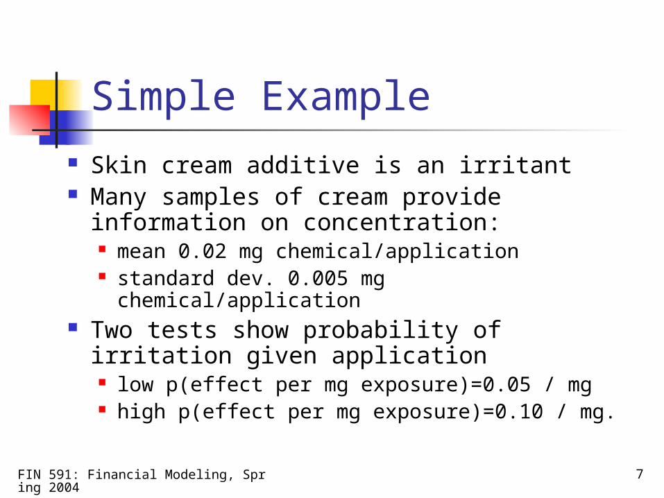
Simple Example Skin cream additive is an irritant Many samples of cream provide

information on concentration: mean 0.02 mg chemical/application standard dev. 0.005 mg

chemical/application Two tests show probability of irritation

given application low p(effect per mg exposure)=0.05 / mg high p(effect per mg exposure)=0.10 / mg.


8

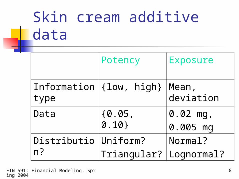
Skin cream additive data

Potency Exposure

Information type

{low, high} Mean, deviation

Data {0.05, 0.10} 0.02 mg, 0.005 mg

Distribution? Uniform?Triangular?

Normal?Lognormal?


9

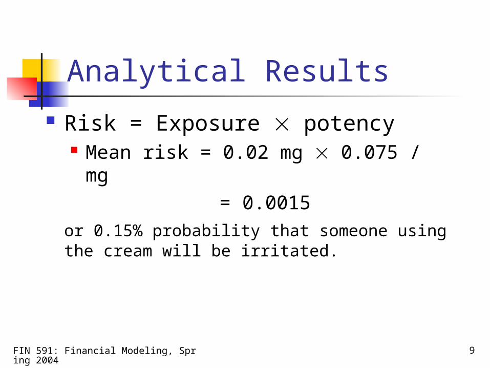
Analytical Results Risk = Exposure potency

Mean risk = 0.02 mg 0.075 / mg = 0.0015

or 0.15% probability that someone using the cream will be irritated.


10

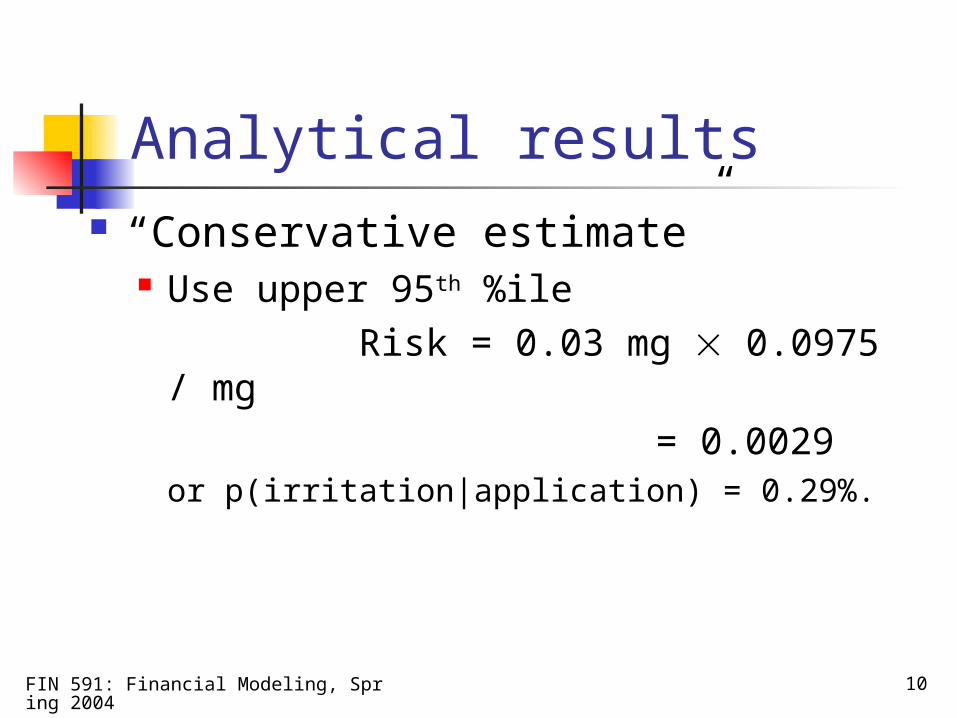
Analytical results “Conservative estimate”

Use upper 95th %ileRisk = 0.03 mg 0.0975 /

mg = 0.0029

or p(irritation|application) = 0.29%.


11

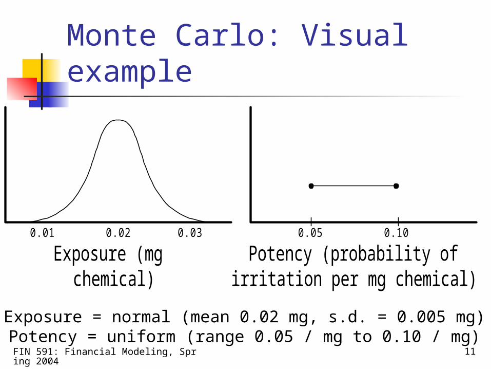
Monte Carlo: Visual example

Exposure = normal (mean 0.02 mg, s.d. = 0.005 mg)Potency = uniform (range 0.05 / mg to 0.10 / mg)

0.02 0.030.01

Exposure (mgchemical)

Potency (probability ofirritation per mg chemical)

0.05 0.10


12

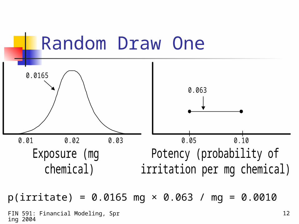
Random Draw One

p(irritate) = 0.0165 mg × 0.063 / mg = 0.0010

0.02 0.030.01



0.05 0.10

0.063

0.0165


13

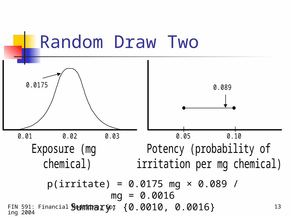
Random Draw Two

p(irritate) = 0.0175 mg × 0.089 / mg = 0.0016

Summary: {0.0010, 0.0016}

0.02 0.030.01



0.05 0.10

0.0890.0175


14

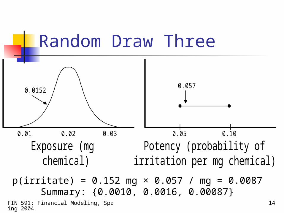
Random Draw Three

p(irritate) = 0.152 mg × 0.057 / mg = 0.0087Summary: {0.0010, 0.0016, 0.00087}

0.02 0.030.01



0.05 0.10

0.0570.0152


15

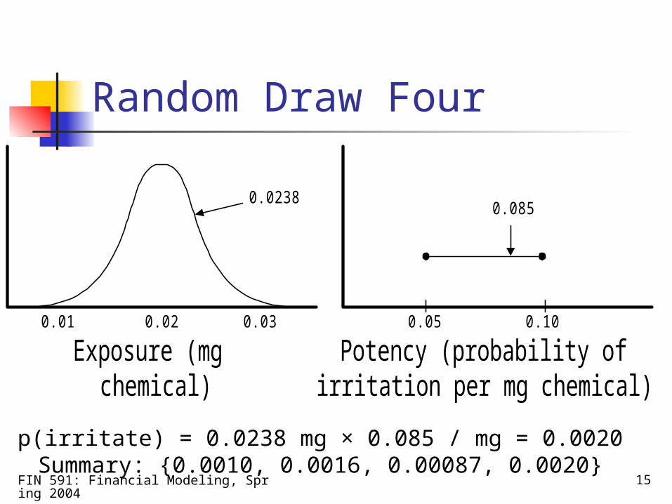
Random Draw Four

p(irritate) = 0.0238 mg × 0.085 / mg = 0.0020Summary: {0.0010, 0.0016, 0.00087, 0.0020}

0.02 0.030.01



0.05 0.10

0.0850.0238


16

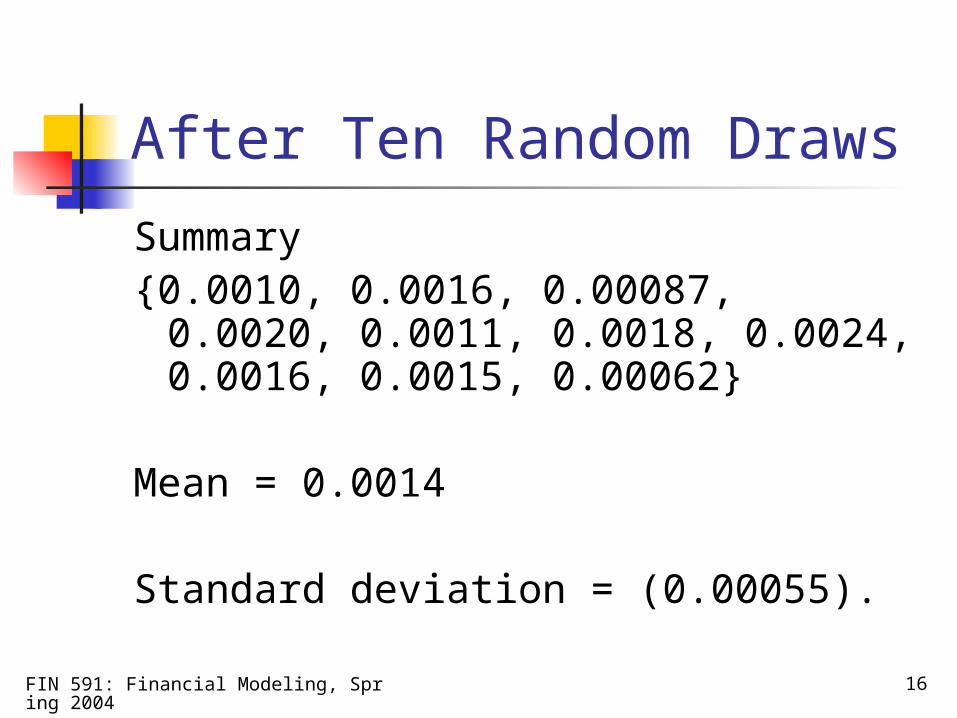
After Ten Random Draws

Summary{0.0010, 0.0016, 0.00087, 0.0020,

0.0011, 0.0018, 0.0024, 0.0016, 0.0015, 0.00062}

Mean = 0.0014

Standard deviation = (0.00055).


17

Using software

Could write this program using a random number generator

But, several software packages exist I use @Risk

User friendly Customizable RNG good up to about 10,000 iterations.


18

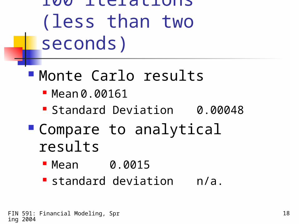
100 iterations (less than two seconds)

Monte Carlo results Mean

0.00161 Standard Deviation 0.00048

Compare to analytical results Mean 0.0015 standard deviation n/a.


19

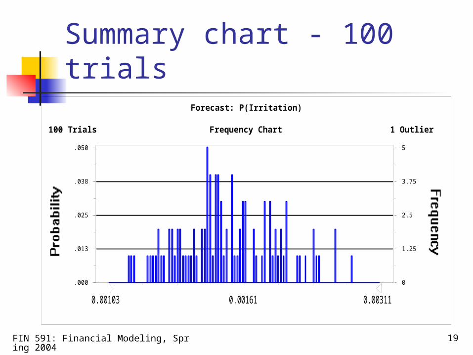
Summary chart - 100 trials

Frequency Chart

.000

.013

.025

.038

.050

0

1.25

2.5

3.75

5

0.00 0.00 0.00 0.00 0.00

100 Trials 1 Outlier

Forecast: P(Irritation)

0.00161 0.003110.00103


20

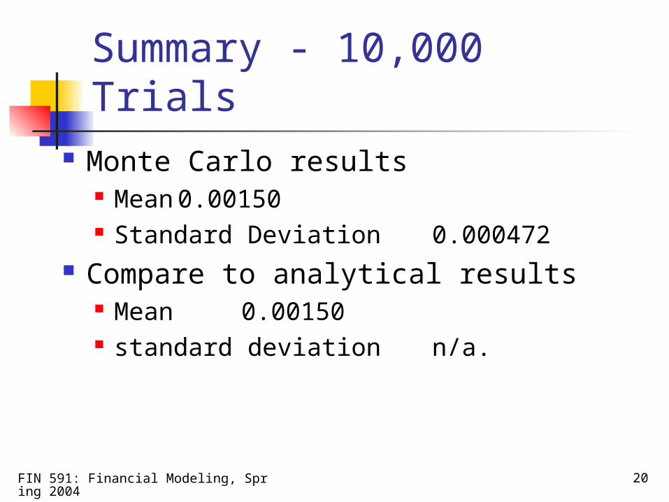
Summary - 10,000 Trials Monte Carlo results

Mean0.00150

Standard Deviation 0.000472 Compare to analytical results

Mean 0.00150

standard deviation n/a.


21

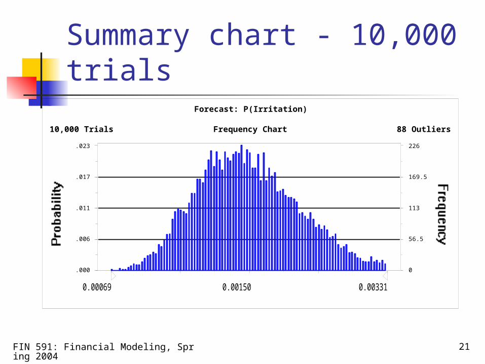
Summary chart - 10,000 trials

Frequency Chart

.000

.006

.011

.017

.023

0

56.5

113

169.5

226

0.00 0.00 0.00 0.00 0.00

10,000 Trials 88 Outliers

Forecast: P(Irritation)

0.00150 0.003310.00069


22

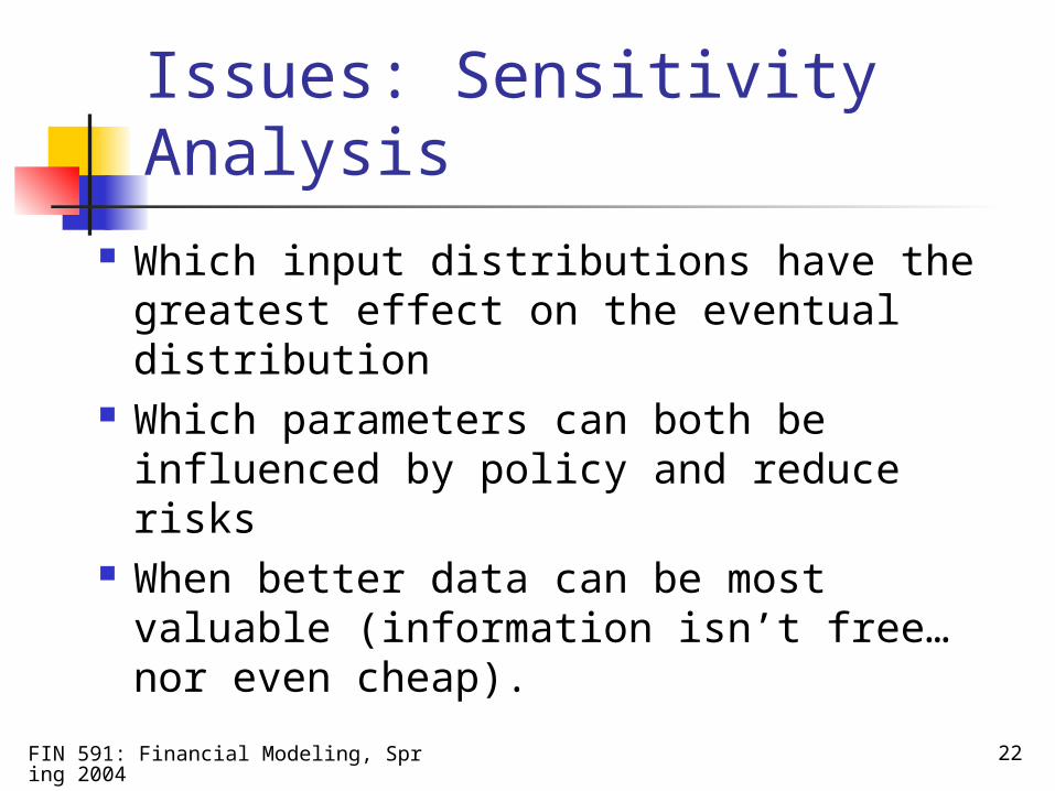
Issues: Sensitivity Analysis Which input distributions have the

greatest effect on the eventual distribution

Which parameters can both be influenced by policy and reduce risks

When better data can be most valuable (information isn’t free…nor even cheap).


23

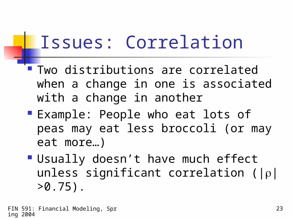
Issues: Correlation Two distributions are correlated when a

change in one is associated with a change in another

Example: People who eat lots of peas may eat less broccoli (or may eat more…)

Usually doesn’t have much effect unless significant correlation (||>0.75).


24

Generating Distributions

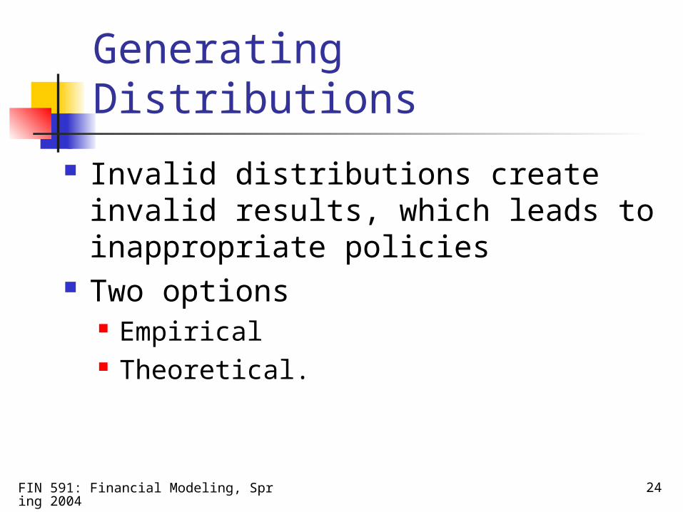
Invalid distributions create invalid results, which leads to inappropriate policies

Two options Empirical Theoretical.


25

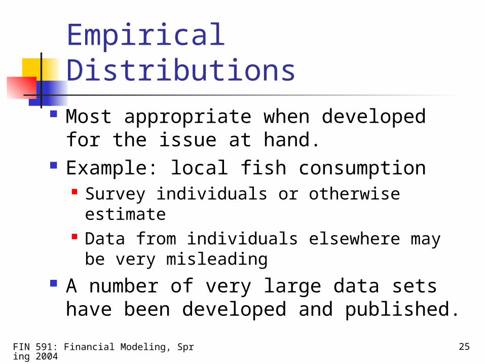
Empirical Distributions Most appropriate when developed for

the issue at hand. Example: local fish consumption

Survey individuals or otherwise estimate Data from individuals elsewhere may be

very misleading A number of very large data sets

have been developed and published.


26

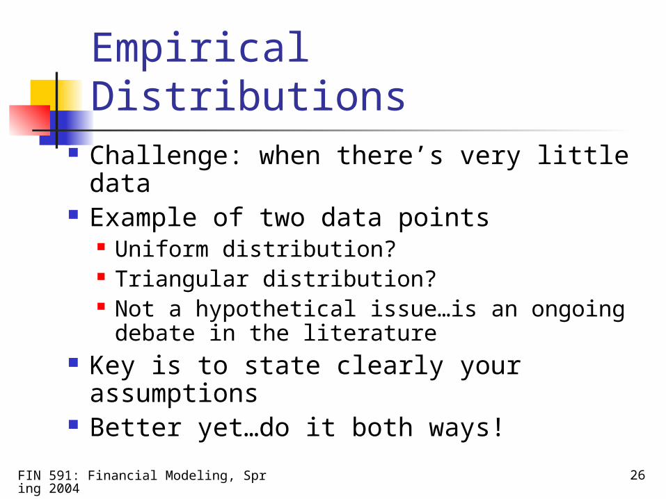
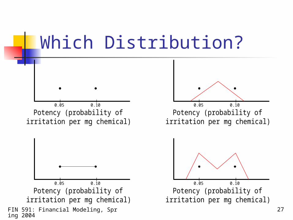
Empirical Distributions Challenge: when there’s very little data Example of two data points

Uniform distribution? Triangular distribution? Not a hypothetical issue…is an ongoing

debate in the literature Key is to state clearly your assumptions Better yet…do it both ways!


27

Which Distribution?


0.05 0.10


0.05 0.10


0.05 0.10


0.05 0.10


28

Random number generation

Shouldn’t be an issue…@Risk is good to at least 10,000 iterations

10,000 iterations is typically enough, even with many input distributions.


29

Theoretical Distributions

Appropriate when there’s some mechanistic or probabilistic basis

Example: small sample (say 50 test animals) establishes a binomial distribution

Lognormal distributions show up often in nature, particular economics/business.


30

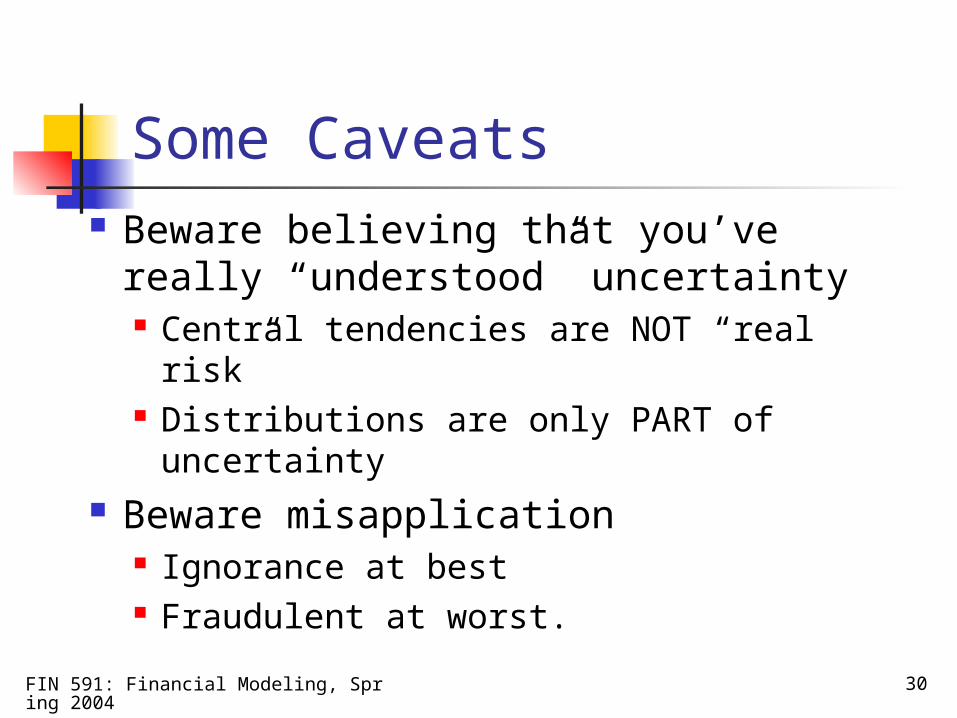
Some Caveats Beware believing that you’ve really

“understood” uncertainty Central tendencies are NOT “real risk” Distributions are only PART of

uncertainty Beware misapplication

Ignorance at best Fraudulent at worst.


31

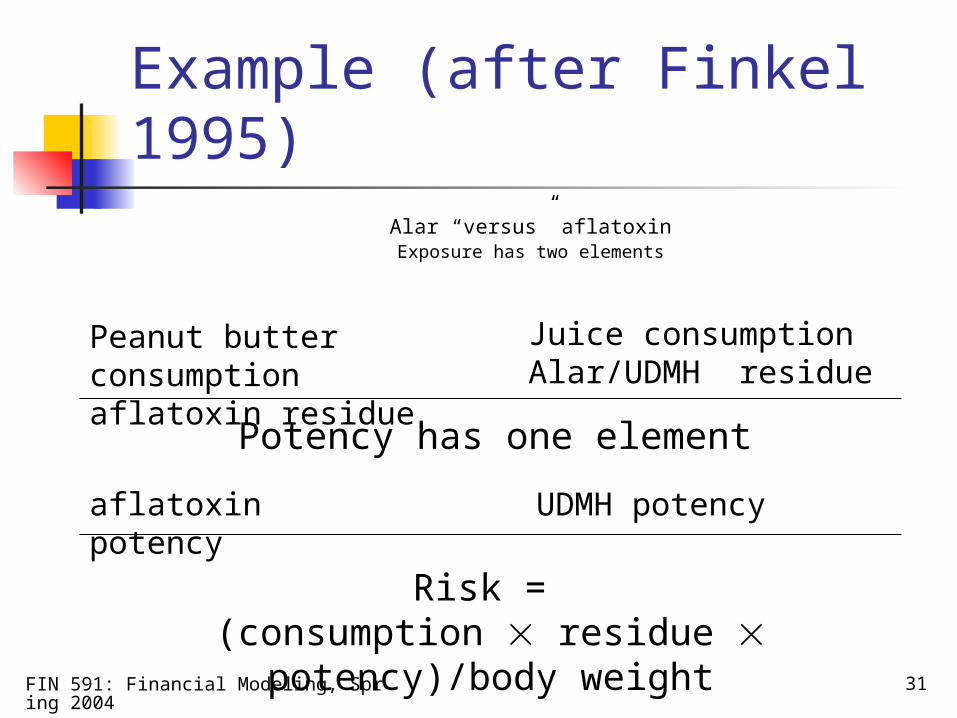
Example (after Finkel 1995)

Alar “versus” aflatoxinExposure has two elements

Peanut butter consumptionaflatoxin residue

Juice consumptionAlar/UDMH residue

Potency has one element

aflatoxin potency UDMH potency

Risk = (consumption residue potency)/body weight


32

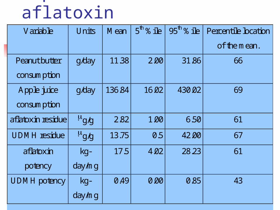
Inputs for Alar & aflatoxinVariable Units Mean 5th %ile 95th %ile Percentile location

of the mean.

Peanut butter

consumption

g/day 11.38 2.00 31.86 66

Apple juice

consumption

g/day 136.84 16.02 430.02 69

aflatoxin residue g/g 2.82 1.00 6.50 61

UDMH residue g/g 13.75 0.5 42.00 67

aflatoxin

potency

kg-

day/mg

17.5 4.02 28.23 61

UDMH potency kg-

day/mg

0.49 0.00 0.85 43


33

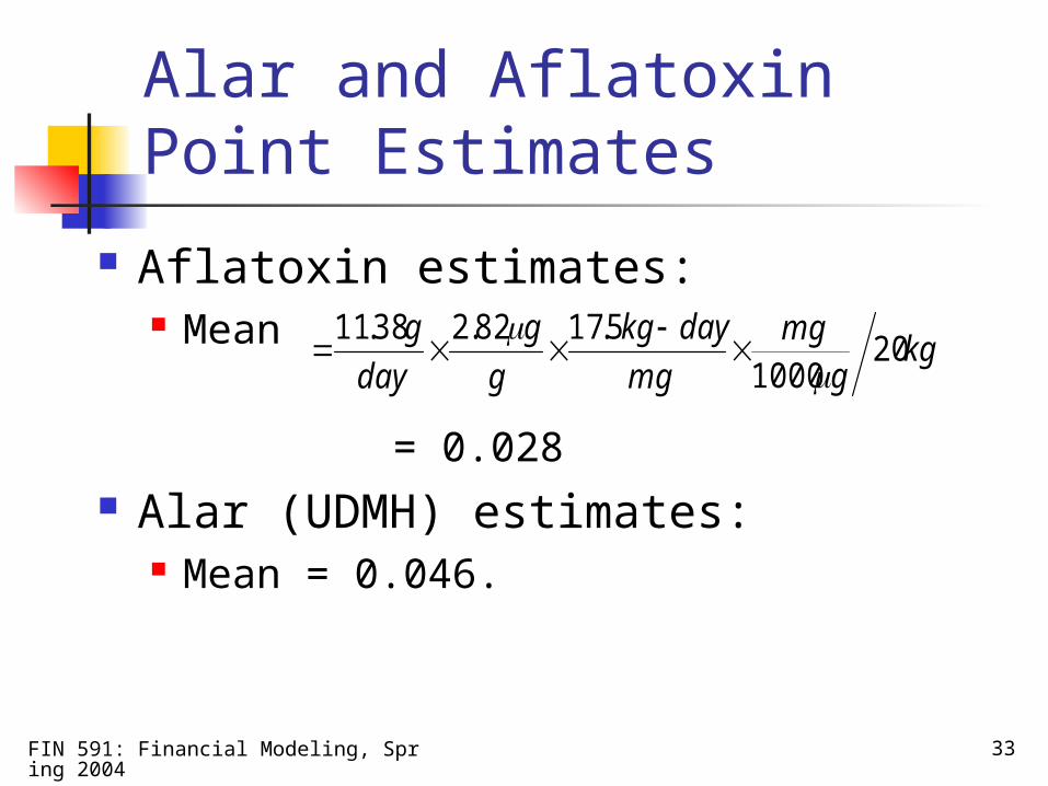
Alar and Aflatoxin Point Estimates

Aflatoxin estimates: Mean

= 0.028 Alar (UDMH) estimates:

Mean = 0.046.

kgg

mg

mg

daykg

g

g

day

g20

1000

5.1782.238.11


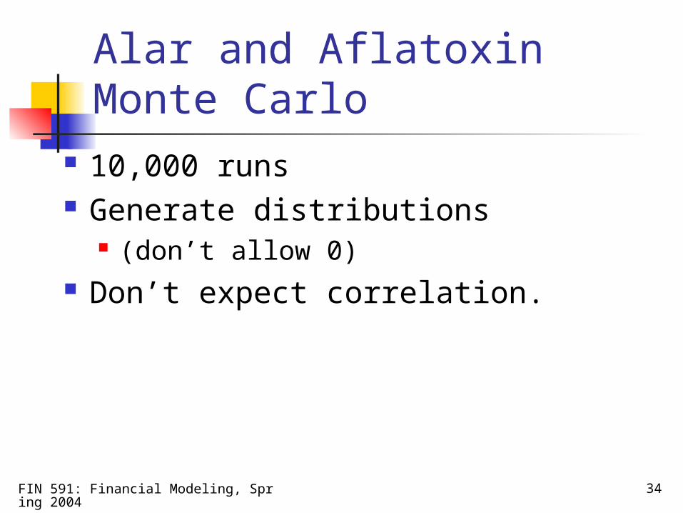
34

Alar and Aflatoxin Monte Carlo

10,000 runs Generate distributions

(don’t allow 0) Don’t expect correlation.


35

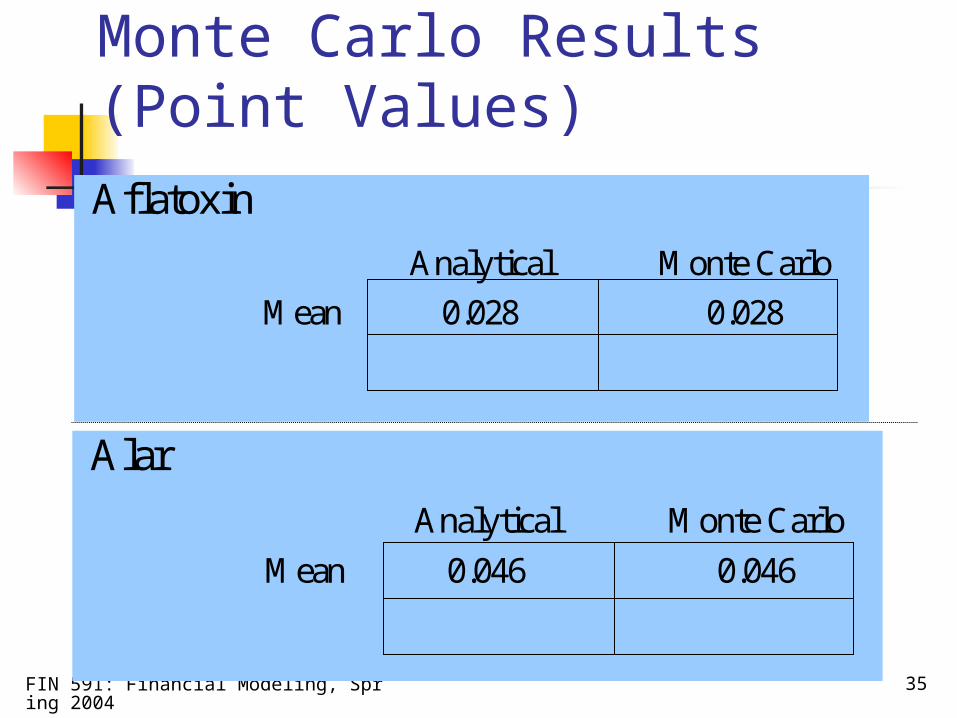
Aflatoxin and Alar Monte Carlo Results (Point Values)

Aflatoxin

Analytical Monte Carlo Mean 0.028 0.028

Alar

Analytical Monte Carlo Mean 0.046 0.046


36

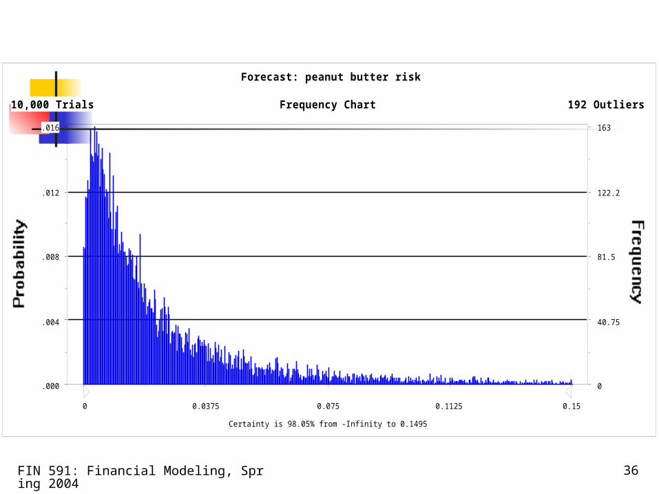
Frequency Chart

Certainty is 98.05% from -Infinity to 0.1495

.000

.004

.008

.012

.016

0

40.75

81.5

122.2

163

0 0.0375 0.075 0.1125 0.15


Forecast: peanut butter risk


37

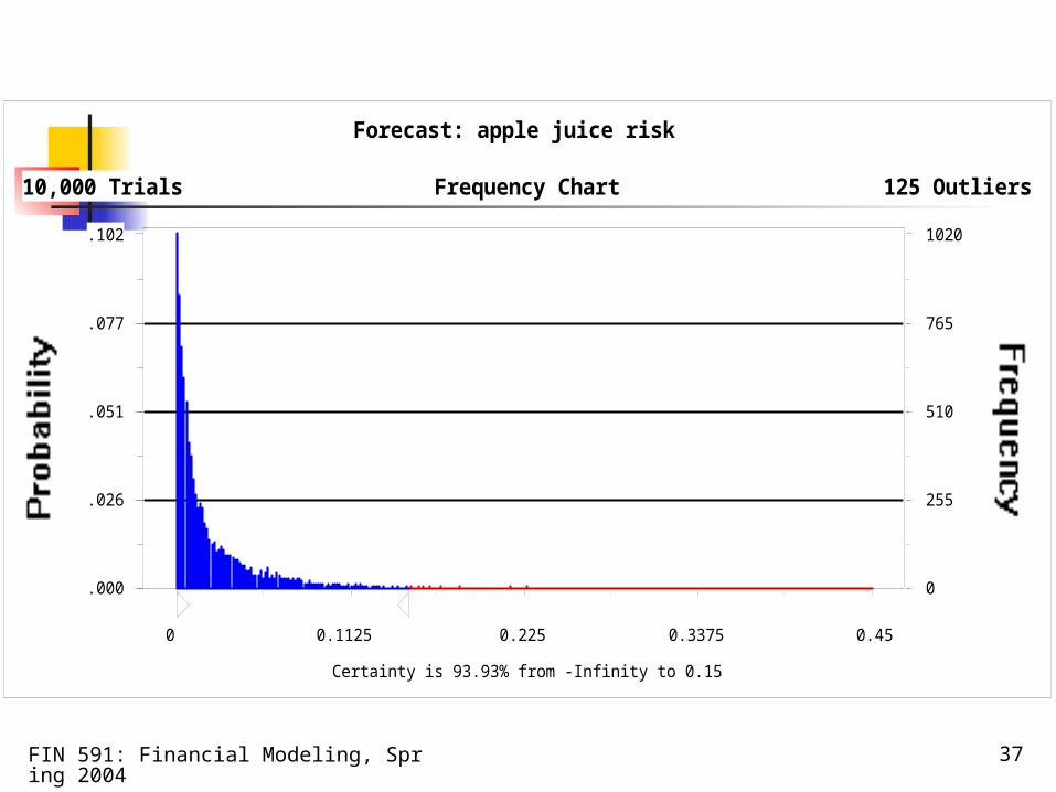
Frequency Chart


.000

.026

.051

.077

.102

0

255

510

765

1020

0 0.1125 0.225 0.3375 0.45


Forecast: apple juice risk


38

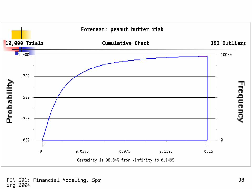
Cumulative Chart


.000

.250

.500

.750

1.000

0

10000

0 0.0375 0.075 0.1125 0.15


Forecast: peanut butter risk


39

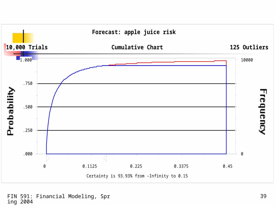
Cumulative Chart


.000

.250

.500

.750

1.000

0

10000

0 0.1125 0.225 0.3375 0.45


Forecast: apple juice risk


40

End

Documents

Monte Carlo Analysis A Technique for Combining Distributions