Monopolistic competition, increasing returns to scale, and the

qWe would like to thank Parantap Basu, Russell Cooper, Dean Corbae, Paul Evans,Marvin Goodfriend, Peter Howitt, Nelson Mark, Douglas Mitchell, Bartholomew Moore, ShashiMurthy, James Peck, Argia Sbordone, Stephanie Schmitt-Grohe, John Wald and seminarparticipants at Colgate University, Fordham University, Ohio State University, Rutgers University,and the North American Econometric Society Meeting for helpful comments. We are especiallygrateful to an anonymous referee and the editor (Robert King) for the generous comments andsuggestions which have led to a substantial improvement in the quality of the paper. We also thankJang-Ting Guo for kindly providing part of the data used in this study. The usual disclaimerapplies.

*Corresponding author. Tel.: #1-973-353-1146; fax: #1-973-353-1233.E-mail address: [email protected] (Y. Wu).

Journal of Monetary Economics 46 (2000) 417}440

Monopolistic competition, increasing returnsto scale, and the welfare costs of in#ationq

Yangru Wu!,*, Junxi Zhang"

!Department of Finance and Economics, Faculty of Management, Rutgers University, Newark,NJ 07102-1820, USA

"University of Hong Kong, Hong Kong

Received 9 February 1998; received in revised form 1 November 1999; accepted 11 November 1999

Abstract

This paper introduces monopolistic competition and increasing returns to scaleinto a monetary real business cycle (RBC) model to re-estimate the welfare costsof in#ation. We "rst calibrate the model and show that it is capable of generatingthe observed aggregate #uctuations even when there are no shocks to the fundamentals.In particular, we demonstrate that this model matches the stylized U.S. business cyclesfacts as well as two more standard models. Then, we "nd that in this model the scaleparameters and the intensity of competition signi"cantly a!ects the welfare cost ofin#ation. Speci"cally, the cost is considerably higher than that in a standard RBC modelwith competitive markets and constant returns. Moreover, the stronger the increasingreturns and the less intense the competition, the higher the welfare costs. These results are

0304-3932/00/$ - see front matter ( 2000 Elsevier Science B.V. All rights reserved.PII: S 0 3 0 4 - 3 9 3 2 ( 0 0 ) 0 0 0 3 6 - 2

1Gomme argues that this result is largely due to the endogenous labor-leisure choice. It should benoted, however, that Gomme studies the welfare costs of in#ation in a monetary version of the Lucas(1988) model with endogenous growth but omits the spillover e!ects in the accumulation of humancapital. In a recent paper, Wu and Zhang (1998) reexamine this issue by considering such externale!ects and "nd that the costs are substantially higher than those documented by Gomme.

2Den Haan (1990), in a model requiring time for cash exchange as well as for credit-type exchange,reports a comparatively high cost of 4.68% for the economy going from 0% to a 5% monetary growth.

con"rmed in a number of model speci"cations. ( 2000 Elsevier Science B.V. All rightsreserved.

JEL classixcation: E31; E32; E37

Keywords: Welfare costs of in#ation; Monopolistic competition; Dynamic indeterminacy

1. Introduction

The cash-in-advance economies of Lucas (1980,1984) and Lucas and Stokey(1983,1987), under the maintained hypothesis of competitive markets and con-stant returns to scale, have been widely used in monetary theory. One empiricalapplication concerns the assessment of the welfare costs of in#ation, and thereexists a substantial literature on it. Within such a framework, estimates of thewelfare costs of moderate in#ation are generally modest or small. Cooley andHansen (1989) report a cost of 0.387% of GNP for a 10% annual money growthrate. Later, Cooley and Hansen (1991) con"rmed basically the same "nding inanother model with cash and costless credit and the presence of labor andcapital taxation. Such a magnitude is also consistent with other estimates. Usingwelfare triangles, Fischer (1981) obtains a cost of 0.3%, while Lucas (1981) o!ersa "gure of 0.45%.

Several subsequent researchers have attempted to re-address this issue byconsidering alternative speci"cations in the cash-in-advance economy. Unfortu-nately, they generate either incompatible or con#icting results. Among them,two papers, which take di!erent routes, have reported quite di!erent results. The"rst paper, by Gomme (1993), extends the Lucas-Stokey (1983) cash-in-advanceeconomy to include endogenous growth. With an endogenous labor-leisuretrade-o!, Gomme obtains, quite surprisingly, extremely small welfare costs forvarious monetary growth rates. For example, a 10% money growth rate resultsin a welfare cost of less than 0.03% of income.1 The second paper, by Gillman(1993), modi"es the Lucas-Stokey economy by specifying an exchange functionthrough which the consumer decides whether to use cash or costly credit topurchase a good. It is shown that the consumer faces higher welfare costs than0.4% in standard cash-in-advance economies. The magnitude is as high as2.19% for a 10% monetary growth rate in this costly credit economy.2

418 Y. Wu, J. Zhang / Journal of Monetary Economics 46 (2000) 417}440

3Our use of noncompetitive markets and increasing returns economies is motivated by some ofthe recent empirical studies. For example, Hall (1986, 1988, 1990) suggests that increasing returnsand monopoly power may better describe the real-world economies, which can potentially accountfor a number of macro issues, such as the observed correlation of the Solow residuals with somemeasures of aggregate demand shifts. Moreover, empirical results suggesting the presence ofmonopoly markups or externalities are also obtained in the literature, for instance, Domowitz et al.(1988), Baxter and King (1991), and Caballero and Lyons (1992). Indeed, there are a large number ofbusiness cycle models that include an imperfectly competitive element; see the citations by Farmerand Guo (1994) for details.

4 In Hornstein's model, increasing returns arise from the introduction of an &overhead cost'component, rather than the usual assumption that the rate of return in production sums to morethan one.

All these studies, however, assume perfect competition, constant returns toscale and price taking behavior by the producers and consumers. This paperattempts to study the welfare cost issue in a framework with two new elements} monopolistic competition and increasing returns to scale.3 In such a frame-work, a technical issue needs to be addressed at "rst. It is known that theunderlying economy in a standard monetary RBC model can be characterizedby a saddle-path equilibrium. Under the alternative hypothesis of monopolisticcompetition and increasing returns to scale, this property can only be main-tained if increasing returns are mild, such as in a real model by Hornstein(1993).4 However, when increasing returns are su$ciently strong, the abovedeparture from the standard paradigm may alter the stability of the steady stateand lead to potentially more radical implications. More speci"cally, sucha model, as in Benhabib and Farmer (1994), displays an indeterminate steadystate (i.e., a sink), and one may exploit this indeterminacy to generate a model ofaggregate #uctuations that is solely driven by self-fulxlling beliefs, also known assunspots or animal spirits in the literature. Farmer and Guo (1994) show thatwhen the Benhabib and Farmer (1994) model is calibrated to the post-War U.S.data, not only is it a theoretical curiosity for sunspots to drive business cycles,but it occurs well within the range of parameter values that are empiricallyrealistic and plausible. In other words, it is possible for purely extrinsic uncer-tainty to induce the magnitude of #uctuations that we observe.

In our model, there are a continuum of monopolistically competitive inter-mediate goods producers who face increasing returns technologies. As in recentstudies of this type, increasing returns are allowed to vary to a particular stagewhere indeterminacy may occur. In this case, even if there is no fundamentaluncertainty whatsoever, economic aggregates may still undergo irregular #uctu-ations as a direct result of the self-ful"lling beliefs of rational forward lookingindividuals. We show that this economy captures reasonably well the stylizedfacts of the U.S. business cycles as the standard monetary RBC model anda model with mild increasing returns and a saddle point.

Y. Wu, J. Zhang / Journal of Monetary Economics 46 (2000) 417}440 419

We then derive a closed-form welfare cost function, and "nd that both thescale parameters and the intensity of competition signi"cantly a!ect the welfarecost function. One of the main results of the current paper is that the welfare costin this model with monopolistic competition and increasing returns is consider-ably higher than that in the Cooley}Hansen (1989) model with competitivemarkets and constant returns. In terms of magnitude, a 10% money growthleads to a welfare cost of 3.4% in our model as opposed to 0.4% in the Cooley}Hansen model. Moreover, the stronger the increasing returns, the higher thewelfare cost; and the less the intensity of competition among "rms, the higher thewelfare cost. These "ndings also demonstrate that the quantitative e!ects ofanticipated in#ation may have been substantially underestimated if the underly-ing economy exhibits characteristics of non-standard features.

To investigate the robustness of our results, we go on to examine them withrespect to a number of model speci"cations. First, we consider an alteration inthe preferences of the representative agent to capture the more realistic feature ofa varying marginal utility of leisure. Second, we expand our form of moneydemand to also include "rms' investment in the cash-in-advance constraint.Finally, we modify our model by using a shopping-time transactions technologyof money demand. It is then found that our conclusion of higher welfare costs inthe paradigm of monopolistic competition and increasing returns is con"rmedunder each variant, thereby suggesting that our results are quite robust and general.

The remainder of the paper is organized as follows. Section 2 presents theeconomic environment and de"nes the stationary equilibrium. In Section 3, westudy the dynamics and expectational shocks. The model is then parameterizedand calibrated, and is subject to a number of diagnoses in Section 4. Section5 reports the welfare costs of in#ation for our basic model speci"cation andcompares them with those implied by two more standard models. The welfarecosts in models with intermediate parameter values are also studied. Section6 examines three alternative speci"cations. Finally, some concluding remarksare o!ered in Section 7.

2. A basic model with monopolistic competition and strong increasing returns

2.1. The economic environment

The model economy is populated by a large number of individuals, each withthe same preference ordering. Utility is derived from consumption, c

t, and

leisure, lt, or equivalently work e!ort, h

t. (Variables are expressed in per capita

terms.) The utility function is time separable and has a constant rate of intertem-poral preference, o

E0

=+t/0

o t;(ct, h

t), o3(0,1), (1)


where E is the mathematical expectation operator. This function ; is assumedto be strictly concave and twice continuously di!erentiable, satisfying;

c'0,;

h(0,;

cc(0,;

ch40,;

hh(0, and the Inada conditions.

The representative agent enters period t with physical capital, kt, and nominal

cash balances, mt. As is standard practice in the literature, we assume that in the

beginning of the period, the state-of-the-world is revealed; namely, the current-period productivity shock, Z

t, and gross per-capita growth rate of money, g

t, are

revealed. The government's only role involves controlling the money supplyprocess: it administers a redistributive program by making a lump-sum transferof its seigniorage revenues, q

t, to the individual in the form of nominal balances.

In addition to the budget constraint to be speci"ed later, the representativeagent also faces a cash-in-advance constraint (CIA) towards its purchases of thenonstorable consumption good. Namely, such purchases are "nanced directlyby the beginning-of-period cash balances, which are the sum of balances fromthe period, m

t, and transfers from the government, q

t

ptct4m

t#q

t, (2)

where ptis the price level in period t.

Since a key feature of our model lies in its organizational structure whichinvolves monopolistic competition and increasing returns, the individual in-come comes from not only physical capital, k

t, and labor e!ort, h

t, but also

ownership of "rms in the form of positive pro"ts, nt. Income can be spent on

either consumption, capital investment (itin real terms), or the accumulation of

nominal cash balances to take into next period (mt`1

). Let the rate of return (netof depreciation) on capital be r

t, and the wage rate be w

t. Then the budget

constraint is

ct#i

t#m

t`1/p

t4w

tht#r

tkt#n

t#(m

t#q

t)/p

t, (3)

where investment and capital satisfy the following law of motion:

kt`1

"(1!d)kt#i

t. (4)

The constant parameter d3[0,1] is the depreciation rate of physical capital.On the production side, following Benhabib and Farmer (1994), there are

a continuum of monopolistically competitive intermediate goods producers,indexed by j3(0,1), who face increasing returns technologies. Final output,produced in a competitive sector, is given by

>"CP1

0

>(j)jdjD1@j

, (5)

where j3(0,1) measures the degree of monopoly power in the markets forintermediate products. The smaller the value of j, the higher the markup, andthe higher the monopoly pro"ts. Throughout this paper, we shall use capital


5 In Section 4, our calibration of the model takes the same parameter values from Farmer andGuo (1994). Speci"cally, we take j"0.58, a"0.23, b"0.7, and hence a#b(1 is satis"ed;moreover, these numbers imply that a"0.4, b"1.21, and so a#b'1.

letters to denote (per-capita) economy-wide variables, and lower-case letters todenote (per-capita) individual variables. For ease of exposition, we deliberatelykeep them distinct from each other, although in equilibrium they equalize. Theproduction function for intermediate good j is assumed to possess theCobb}Douglas form,

>t( j)"Z

t( j)K

t( j)aH

t( j)b, a, b'0, a#b'1, (6)

where Zt( j) is a productivity shock. To keep things simple, we follow Benhabib

and Farmer (1994) by assuming that the same technology is used to produceeach intermediate good. Under this symmetry assumption, we haveZ

t( j)"Z

t,>

t( j)">

t, K

t(j)"K

t, and H

t( j)"H

t. Thus, the aggregate produc-

tion function can be expressed as

>t"Z

tKa

tHb

t. (7)

The productivity shock Ztevolves according to

Zt"Zh1

t~1ut, h

13(0,1), Z

0is given. (8)

The autocorrelation of the productivity shock, Zt, is intended to capture the fact

that U.S. GNP requires at least a second-order representation suggested by thedata. In two of the models below, the innovation, u

t, is speci"ed as an i.i.d.

random variable which follows a lognormal distribution with mean zero, whilein the other model Z is speci"ed as a constant equal to unity.

Under the hypothesis that factor markets are competitive, standard "rst-order conditions of the representative "rm lead to

rt"a>

t/K

t, w

t"b>

t/H

t, a"ja, b"jb, (9)

where a and b are the capital and labor shares in national income, respectively.Notice that in this monopolistically competitive model, the sum of factor sharesof national income is less than one, a#b(1, thereby allowing for the presenceof positive pro"ts.5 By contrast, in a model with competitive input markets andconstant returns, a#b"1, a"a, and b"b.

Finally, the budget constraint for the government is

qt"(g

t!1)M

t, (10)

where Mt

is per-capita money stock (exogenous). Its gross growth rate, gt,

evolves according to

gt"gh2

t~1vt, h

23(0,1), g

0is given, (11)


where vtis a random shock, which follows a lognormal distribution with mean

zero. For the model economy, we also consider a special case in which gt

isa constant. This then is qualitatively equivalent to the standard RBC modelwithout monetary shocks.

2.2. Market equilibrium

In the model laid out above, it is observed that some variables display growthin equilibrium; e.g., with a growing money supply, nominal prices are clearly notstationary. To ensure the existence of stationary market equilibria, we need totransform them into variables that are scaled appropriately to eliminate growth.To this end, denote m

M"m/M, p

M"p/M, and q

M"q/M, where the super-

#uous time subscripts have been dropped; also denote a prime (@) as the next-period value, and the aggregate state as S"(Z, g, K). Then prices, distributedpro"ts and government transfers can presumably be expressed as functions ofthe aggregate state; that is, p

M"p

M(S), r"r(S), w"w(S), n"n(S), and

qM"q

M(S). As a result, the problem faced by the representative agent is to

choose consumption (c), labor e!ort (h), stock of physical capital (k@), and cashbalances (m@

M), so as to solve the following dynamic programming problem:

<(k,mM

,S)" maxc,h,k{,m@

M

M;(c, h)#oE[<(k@,m@M

, S@)D(k,mM

,S)]N, (12)

s.t. c#k@#gm@M

/pM

(S)

4w(S)h#[1!d#r(S)]k#n(S)#[mM#q

M(S)]/p

M(S),

(13a)

pM

(S)c4mM#q

M(S), (13b)

S@"S(Z(S, u@), g(S, v@),K(S)). (13c)

De,nition. A stationary market equilibrium consists of policy functionsc(s), h(s), k(s), m@

M(s), K(S), and H(S), where s"(k, m

M, S); pricing functions

pM

(S), r(S), and w(S); a pro"t function n(S); and a transfer function qM

(S) suchthat (i) the functions <, K,H, and p

Msatisfy (12) and c, h, k, and m@

Mare the

associated policy functions; and (ii) the money market, the labor market, thecapital market, and the goods market all clear: m

M"m@

M"1, h"H, k"K,

and

c#k@">#(1!d)k. (14)

In what follows, the attention will be focused on circumstances under whichthe CIA constraint always holds with equality. As is well known, a su$cientcondition for this constraint to be binding is that the gross growth rate of


6 In Section 4 on empirical results, this is equivalent to assuming that the annual in#ation rate isequal to or higher than !4%, which is a reasonable assumption.

money, gt, always exceeds the discount factor, o.6 Consequently, the conditions

characterizing this dynamic optimum include the market-clearing conditions(notably (14)) and

;h(c, h)/w"oE[(1!d#r@);

h(c@, h@)/w@], (15a)

g;h(c, h)/(p

Mw)"oE[;

c(c@, h@)/p@

M], (15b)

k@"Zkahb#(1!d)k!g/pM

. (15c)

Notice that Eq. (15c) is the goods market-clearing condition or resource con-straint expressed in per-capita form when the individual CIA constraint isbinding.

3. Dynamics and expectational shocks

In this section, we study the transitional dynamics implied by the model bytaking a linear approximation of the system around an initial stationary equilib-rium. To accomplish this, it remains to specify the instantaneous utility function.As in related studies, it is parameterized as

;(c, h)"ln c!Bh, (16)

where B is a constant parameter. The use of such a functional form can bejusti"ed by the following two reasons. First, this form of indivisible labor isstandard in the literature, see, e.g., Hansen (1985), Rogerson (1988) and Cooleyand Hansen (1989) among others. With the form like (16), we can compare theimplied welfare costs of in#ation in our model economy of monopolistic com-petition and strong increasing returns with those in existing models of competi-tive markets and constant returns. Second, the informational requirements aresubstantially reduced by this simpli"cation. Namely, Eq. (15b) can be eventuallysimpli"ed to involve only one unknown, p

M; as a result, solving for p

Mand

substituting into Eq. (15c) will leave the dynamic system with only two di!erenceequations in k and h.

Z~1k~ah1~b"E[oa(k@)~1h@#o(1!d)(Z@)~1(k@)~a(h@)1~b], (17)

k@"Zkahb#(1!d)k!(ob/B)Zkahb~1E(1/g@). (18)


7More precisely, given appropriate parameterization, we can show that in our multidimensionalsystem, the two roots associated with capital and hours worked are complex conjugates. See thediscussion in the following section.

By setting the steady-state values ZH"1 and gH"g (a constant), the steady-state values of kH and hH can be readily obtained:

hH"ob

gB

1!o(1!d)

1!o(1!d)!aod, kH"C

ao1!o(1!d)

(hH)bD1@(1~a)

. (19)

An additional equation speci"es how the steady-state values of cH and pHM

areinterrelated:

cH"g/pHM"(ob/gB)(kH)a(hH)b~1. (20)

Next the dynamics of our stochastic economy are described as follows. Leta circum#ex denote the deviation of a variable from its steady-state valueexpressed as a percentage of that value, e.g., kK "(k!kH)/kH. First, we takea "rst-order Taylor series approximation to Eqs. (8), (11), (17) and (18) aroundthe steady state. We then carry out some straightforward algebraic manipula-tion on the linearized equations by exploiting the cross-equation restrictions.The resulting solution of this system can be written in the form

CkK @hK @ZK @g( @D"AC

kKhKZKg( D#DC

u( @

v( @

e( @hD , (21)

where e( @h,h@!E(h@) and A and D are, respectively, 4]4 and 4]3 matrices

de"ned in a technical appendix available upon request. The term e( @h

representsdisturbances to labor e!ort that have zero-conditional mean at time t. In theremainder of this paper, e( @

his interpreted as a self-ful"lling belief.

It is clear that the dynamic characteristics of the decision rules (21) around thesteady state are governed by the transition matrix, A. In standard RBC frame-works, this matrix possesses four real eigenvalues, one of which is greater thanunity in absolute value, while the other three are smaller than one in absolutevalues. In this case, the system (21) implies a saddle point equilibrium witha unique convergent path. In this paper, however, if the returns to scale arestrong, then all roots of the matrix A lie inside the unit circle.7 Therefore, similarto Farmer and Guo (1994) who introduce increasing returns to a real economy,our model generates an important implication: its steady state has a sink withmultiple paths converging towards it, and hence the belief shock to the labore!ort equation, e( @

h, inevitably a!ects its dynamic path and may be an important


8As shown in Benhabib and Farmer (1994), the key feature which causes a change in the stabilityof the steady state is the fact that strong increasing returns imply that the labor demand curve mayslope up and is steeper than the labor supply curve. It can be readily veri"ed that the slopes of thedemand and supply curves are b!1 and 0, respectively. So, the necessary condition for indetermin-acy requires b'1.

9An alternative model would be to assume price-taking behavior but incorporate increasingreturns by externalities, similar to the one studied in Baxter and King (1991) without money.

source of business cycle #uctuations. In the extreme case of no fundamentalshocks, i.e., u( @"v( @"0, strong increasing returns can induce indeterminacy ofthe equilibrium, leaving the belief shocks a sole source of #uctuations that canmagnify the e!ects of other shocks.8 Therefore, we refer to this model as the&sunspot' model.

To gain further insights about the e!ects of introducing strong increasingreturns, we calibrate and simulate the sunspot model and also two compatibleversions of the above system, both with the dynamic property that all roots ofthe transition matrix, A, are real, with one larger than one in absolute value andthe others less than one in absolute values. The "rst one is a standard monetaryRBC model with competitive markets and a technology that satis"es constantreturns to scale, whereas the second, although with monopolistically competi-tive markets, exhibits mild increasing returns to scale and saddle point dynam-ics.9 These two economies are termed as the &competitive' and &saddle' economies,respectively. The di!erence between this second economy and ours is that oureconomy displays an indeterminate approach to the steady state, which, asrecognized by Farmer and Guo (1994), implies that the dynamics of ourlinearized model no longer provide enough restrictions to uniquely determinea rational expectations equilibrium in terms of fundamentals.

For these two models, using the saddle-path property as a restriction, thedecision rules (21) can be simpli"ed as follows:

kK @"b11

kK #b12

z(#b13

g( , (22a)

z( @"h1z(#u( @, (22b)

g( @"h2g(#v( @, (22c)

b21

kK #b22

hK #b23

z(#b24

g("0, (22d)

where (22d) is the equation of the saddle. This equation and the constantcoe$cients, b's, are derived in a technical appendix which is available from theauthors upon request. Notably, unlike that in (21), expectational errors,e( @h

vanish in (22), leaving the system to be driven exclusively by fundamentalshocks. Interestingly, (22) implies that the data can be described as a third-ordersystem, while (21) suggests that they can be described as a fourth-order system.


4. Model calibration and diagnoses

In this Section, we provide some simple diagnoses of our sunspot model. As inmost recent studies of this type, the model will be evaluated on how well itaccounts for the observed cyclical properties of the key U.S. macroeconomicvariables. To further investigate the model implications, we also compare it withtwo stylized models, namely, the &competitive' and the &saddle' economiesoutlined in the preceding section.

4.1. Calibration

The parameter values of the model economies are determined by, either usingmicro evidence or matching steady-state values of certain variables with theirlong-run averages observed in the data. The preference parameters are set too"0.99 and B"2.86, the same as in Cooley and Hansen (1989) for a compara-tive study of the two models. The quarterly depreciation rate for the capitalstock, d, is set to 0.025, indicating an annual rate of 10%, as in Kydlandand Prescott (1982) and their followers. For the scale parameters, in the com-petitive economy with constant returns, the capital and labor shares of nationalincome are chosen to be a"0.36 and b"0.64, respectively. In the other twoeconomies with noncompetitive markets and increasing returns, we followFarmer and Guo (1994) in specifying these parameter values. Speci"cally, in thesaddle economy with monopolistic competition and moderate increasing re-turns, the degree of monopoly power, j, is taken to be 0.7, and a"0.43 andb"0.9; in the sunspot economy, the respective values are j"0.58, a"0.4, andb"1.21.

Other parameter values are speci"ed as follows: The mean growth rate ofmoney supply is set to 1.5%, i.e., g6 "1.015. Estimation of the AR(1) process (11)using the growth rate of the U.S. money supply M1 yields h

2"0.60 and

p2"0.0081. Similarly, for the "rst two economies, aggregate #uctuations also

stem from productivity shocks, as governed by Eq. (8). As in related studies, weset the "rst-lag autocorrelation coe$cient, h

1, to 0.95, whilst the standard

deviation of technological innovation, pu, is parameterized so as to match the

standard deviation of output generated by the model economies with thatcomputed from the actual U.S. data. The latter leads to p

u"0.007 for the

competitive economy and pu"0.0046 for the saddle economy.

As for the sunspot economy, we consider two variants: one with a combina-tion of money and expectational shocks and the other with merely expectationalshocks. Such a di!erentiation enables us to study the behavior of nominalvariables in the former. It should be noted that in both circumstances economic#uctuations are largely or entirely propagated by shocks to self-ful"lling beliefs,which are re#ected in the work e!ort equation (see Eq. (21)). For analyticalpurposes, the expectational shock term e( @

h"h@!E(h@) is assumed to follow


a white-noise process with a constant standard deviation peh

. In the absence ofproductivity shocks, this parameter is selected so that the standard deviationof output generated by the arti"cial economy equals its empirical counterpart.As a result, p

eh"0.0103 is taken for the "rst variant, while p

eh"0.0107 is taken

for the second one.The above choice of parameter values implies that for the "rst two economies,

all eigenvalues of the transition matrix, A in Eq. (21), are real numbers. Further-more, the second root is greater than unity in absolute value, while the otherthree are smaller than unity. It is therefore known that each of these twoeconomies can be characterized by a saddle-path equilibrium, suggestingthat the disturbance term to the work e!ort equation can be exclusivelydetermined from the fundamentals of the economy by the cross-equation restric-tion (22d) that places the economy on the stable branch of the saddle.By contrast, for the sunspot economy, increasing returns are su$cientlystrong that all eigenvalues of A lie inside the unit circle. In particular, the tworoots associated with capital and work e!ort are complex conjugates. Asdiscussed in the preceding section, such complex roots are completely capable ofgenerating oscillations in the economy even without serially correlated produc-tivity shocks. Note that in this economy shocks to work e!ort are not onlydetermined by economic fundamentals, but can be driven by self-ful"lling beliefsas well.

4.2. Model diagnoses

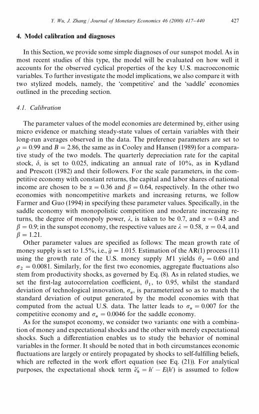
Column (1) of Table 1 presents the standard deviations of major U.S. macro-economic series and their correlations with output (in parentheses). Our data setincludes 151 quarterly observations which span the period from 1954.I to1991.III, all seasonally adjusted. The data on real variables (output, consump-tion, capital stock, investment and hour measures) coincide with those inFarmer and Guo (1994) who kindly provided their data. The series of nominalvariables (M1 money stock, consumer price index and implicit GDP de#ator)are taken from the Citicorp's Citibase data bank. All statistics shown in Table1 have been computed using data that are "rst logged and then detrended by theHodrick}Prescott "lter.

In each model economy, 151 arti"cial observations are simulated usingrespective parameter values chosen above. For the "rst two economies whichpossess a saddle-path equilibrium, innovations to productivity and monetarygrowth are randomly drawn from i.i.d. normal distributions N(0,p2

u) and N(0,p2

v),

respectively; these sequences are then utilized to construct capital andlabor e!ort series according to decision rules (22). For the "rst version of thesunspot economy, we simulate monetary innovations and expectational shocksfrom i.i.d. distributions N(0,p2

v) and N(0,p2

eh), respectively, whereas for the


Table 1Standard deviations and correlations with output for the U.S. and simulated economies!

Variable

QuarterlyU.S. data(1954.I}1991.III)(1)

Competitivemodel(2)

Saddlemodel(3)

Sunspotmodel withAR(1) moneygrowth(4)

Sunspot modelwith constantmoney growth(5)

Output 1.74 1.73 1.73 1.73 1.73(1.00) (1.00) (1.00) (1.00) (1.00)

Consumption 0.86 0.68 0.72 0.63 0.40(0.77) (0.64) (0.75) (0.46) (0.79)

Capital stock 0.47 0.48 0.53 0.76 0.75(0.24) (0.05) (0.06) (0.03) (0.07)

Investment 7.78 5.56 6.27 9.37 9.02(0.90) (0.96) (0.95) (0.95) (0.99)

Hours 1 1.51 1.32 1.27 1.43 1.44(0.86) (0.98) (0.97) (0.98) (0.98)

Hours 2 1.68(0.88)

Productivity 1 0.88 0.50 0.54 0.40 0.40(0.49) (0.86) (0.86) (0.77) (0.79)

Productivity 2 0.82(0.30)

Price (CPI) 1.34 2.08 2.11 2.15 0.40(!0.57) (!0.20) (!0.28) (!0.31) (!0.79)

Price (Def ) 0.84(!0.44)

!Notes: (1) Data sources: the U.S. time series of output, consumption, capital stock, investment,hours 1, hours 2, productivity 1 and productivity 2 are taken from Farmer and Guo (1994). The priceseries are from Citicorp's Citibase data bank. (2) Numbers in the "rst lines are standard deviations,while those in the second lines (in parentheses) are correlations with output.

second version, only the expectational shocks are drawn. The decision rulesat work now are the set of (21). Each economy is simulated 100 times andthe averages of the moments are reported in Columns (2)}(5) of Table 1,respectively.

We then perform two diagnoses: volatility and comovement. The results arepresented in Columns (2)}(5) of Table 1. Due to space limitation, the detaileddiscussion is omitted here. In a word, these exercises demonstrate that thesunspot model matches the volatilities and comovements of economic aggreg-ates with about the same degree of precision as the standard monetary RBCmodels. This success gives much credence to the model for the measurement ofwelfare costs of in#ation in the following sections.


5. Welfare costs of in6ation

In this section, we compute the welfare costs of in#ation under our sunspoteconomy and compare these cost measures with those implied under thecompetitive and saddle economies for various growth rates of money supply. Wefollow Cooley and Hansen (1989) in basing the estimates on the steady-stateproperties of the economy with perfect foresight.

We derive the cost measure in conventional fashion. For each model econ-omy, the welfare cost under an alternative money growth rate is expressed asa compensation in consumption in such a way that individuals would be as wello! as if there were no CIA constraint. This measure of the welfare cost isappropriate for economies with competitive markets and constant returns, asthe equilibrium with non-binding CIA corresponds to a Pareto-optimal alloca-tion by the "rst welfare theorem. For the other two economies, in which marketimperfection is a central ingredient, however, it creates a minor conceptualdi$culty, in that the corresponding market equilibrium is no longer Paretooptimal, even though the CIA constraint does not bind. Nevertheless, sucha case remains the best outcome for economic agents since they attain thehighest utility compared to all other possible rates of money growth. We shalltherefore continue to refer to the equilibrium with the non-binding CIA con-straint as the &optimal' solution for all economies.

As noted in Section 3, when the growth rate of money falls below the discountfactor (g6 4o), the CIA constraint is no longer binding. Let cH and hH denote thesteady-state values of consumption and hours worked under this optimalgrowth rate, and cA and hA denote the respective steady-state values under analternative money growth rate. The welfare cost, denoted by *c, is de"ned asfollows:

;(cH, hH)";(cA#*c, hA). (23)

Under the assumption of utility function (16), the welfare cost *c in (23) can beexpressed as the percentages of steady-state consumption and output, respec-tively:

*c

cA"A

gA

o Bb@(1~a)

expC/AogA

!1BD!1, (24)

*c

>A"

jb/ A

*c

cAB"1!o(1!d)!jaod

1!o(1!d) A*c

cA B, (25)

where /"jb[1!o(1!d)]/[1!o(1!d)!jaod] is a constant parameter.To make our results comparable to those in Cooley and Hansen (1989), Table

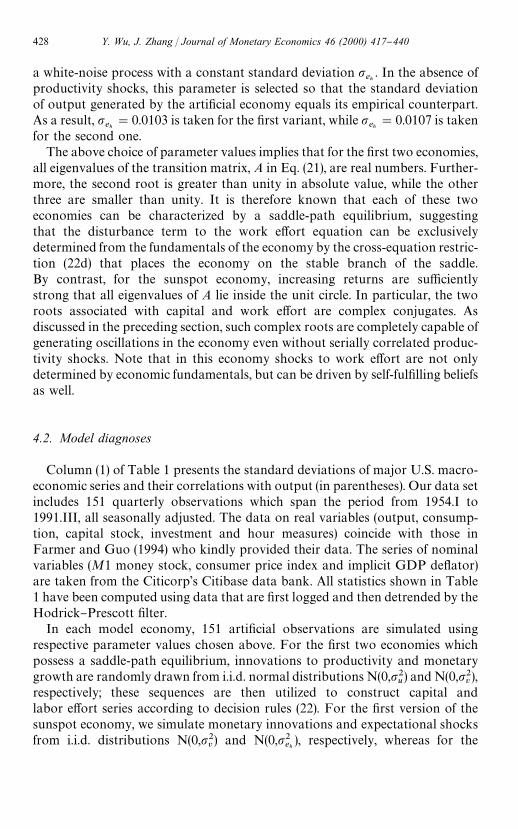
2 presents the welfare costs as well as the steady-state values of some keyvariables for all three model economies under "ve alternative money supply


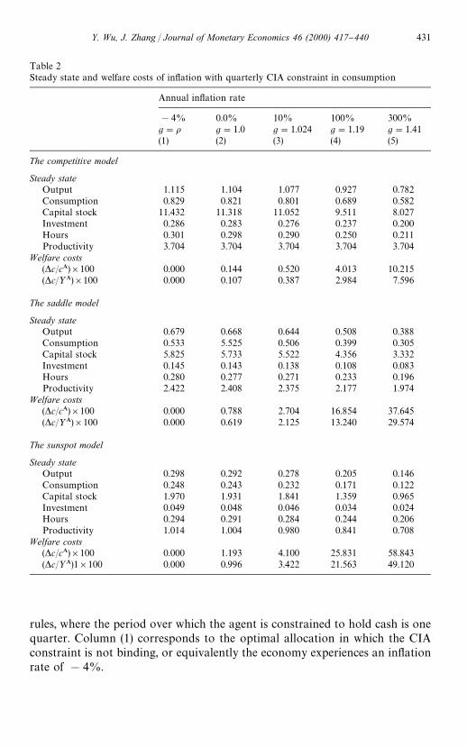
Table 2Steady state and welfare costs of in#ation with quarterly CIA constraint in consumption

Annual in#ation rate

!4% 0.0% 10% 100% 300%g"o g"1.0 g"1.024 g"1.19 g"1.41(1) (2) (3) (4) (5)

The competitive model

Steady stateOutput 1.115 1.104 1.077 0.927 0.782Consumption 0.829 0.821 0.801 0.689 0.582Capital stock 11.432 11.318 11.052 9.511 8.027Investment 0.286 0.283 0.276 0.237 0.200Hours 0.301 0.298 0.290 0.250 0.211Productivity 3.704 3.704 3.704 3.704 3.704

Welfare costs(*c/cA)]100 0.000 0.144 0.520 4.013 10.215(*c/>A)]100 0.000 0.107 0.387 2.984 7.596

The saddle model



The sunspot model


Welfare costs(*c/cA)]100 0.000 1.193 4.100 25.831 58.843(*c/>A)1]100 0.000 0.996 3.422 21.563 49.120

rules, where the period over which the agent is constrained to hold cash is onequarter. Column (1) corresponds to the optimal allocation in which the CIAconstraint is not binding, or equivalently the economy experiences an in#ationrate of !4%.


10Notice that although Gillman's (1993) results are not directly comparable with ours, ourestimates are nevertheless higher. There are two principal di!erences in modeling. First, in his model,steady-state income velocity is allowed to very, while in our model, as in Cooley and Hansen (1989),it is held constant. This can be easily seen by substituting the steady-state income >H"(kH)a(hH)band pH

Mfrom (19) into the velocity measure v

M"pH

M>H. Second, he assumes away physical capital

entirely from the paper.

11As a further con"rmation, we also allow the relevant period over which individuals areconstrained to hold cash to be one month. Although allowing the agent to adjust cash holdings morefrequently substantially relieves the burden placed by the CIA constraint, we nonetheless "nd thatthe above qualitative results remain robust. For example, the "gures for a 10% money growth forthe competitive, saddle, and sunspot economies are 0.112%, 0.669%, and 1.081%, respectively. Thedetailed results are not reported to conserve space.

Two striking results emerge from Table 2: "rst, the welfare costs of variousmoney growth rates in either of the two increasing returns economies areconsiderably higher than those in the Cooley}Hansen (1989) economy; andsecond, the stronger the increasing returns, the higher the welfare costs. Forexample, a 10% money growth results in welfare costs of 2.125 and 3.422% inthe saddle and sunspot economies, respectively, as opposed to 0.387% in theCooley}Hansen economy.10 The signi"cantly higher welfare costs in increasingreturns economies are consistent across all money growth rates.11

To develop a better understanding of the welfare costs of in#ation under thesunspot economy, we consider several variations of the model parameters.

First, for the baseline values of the model parameters, we compute the welfarecosts for the annual in#ation rates ranging from the optimal level of !4}100%,and plot the results in Panel A of Fig. 1. It can be clearly seen that as thein#ation rate increases, both measures of the welfare cost rise monotonically.For example, at the 5% in#ation rate, *c/cA"2.7%, and *c/>A"2.2%.However as the in#ation rate goes up to 10%, *c/cA increases to 4.1% and*c/>A to 3.4%.

One central element of the sunspot economy, which makes it di!erent fromthe traditional neo-classical models, is that the production technology in theintermediate goods sector is subject to strong increasing returns to scale. Oursecond experiment is to investigate how signi"cant returns to scale are ina!ecting the welfare cost of in#ation. Notice that the production technology (7)is described by two parameters a and b. We "x the value of capital elasticity a atits benchmark value of 0.4, while allowing the value of labor elasticity b tochange from 0.6 which corresponds to the constant returns to scale case to 1.21which is the benchmark value used in computing the results in Table 2. All othermodel parameters remain unchanged and the annual in#ation rate is assumed tobe 10%. Panel B of Fig. 1 shows unambiguously the positive relationshipbetween the welfare cost and the value of the scale parameter b. In particular,when the economy is subject to constant returns to scale (b"0.6), the welfarecost for a 10% annual in#ation is *c/cA"2.0%, and *c/>A"1.7%. However,


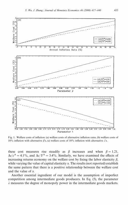
Fig. 1. Welfare costs of in#ation: (a) welfare costs of alternative in#ation rates, (b) welfare costs of10% in#ation with alternative b's, (c) welfare costs of 10% in#ation with alternative j's.

these cost measures rise steadily as b increases and when b"1.21,*c/cA"4.1%, and *c/>A"3.4%. Similarly, we have examined the e!ects ofincreasing returns economy on the welfare cost by "xing the labor elasticity b,while varying the value of capital elasticity a. The results (not reported) establishthe same pattern that there is a positive relationship between the welfare costand the value of a.

Another essential ingredient of our model is the assumption of imperfectcompetition among intermediate goods producers. In Eq. (5), the parameterj measures the degree of monopoly power in the intermediate goods markets.


Therefore, our last experiment studies the relationship between the welfare costof in#ation and the value of j. We calculate the cost of a 10% in#ation forvarious values of j ranging from the baseline value, 0.58, to the perfect competi-tion case, 1.0, while maintaining all other model parameters at the original level.Results presented in Panel C of Fig. 1 plainly indicate that both measures of thewelfare cost monotonically decrease as competition among "rms intensi"es. Inparticular, *c/cA and *c/>A obtain much lower values, 1.0 and 0.7%, respective-ly, as the economy approaches perfect competition, j"1.0.

The above analysis indicates that for a given level of in#ation, the higher thereturns to scale and/or the less competitive the market, the higher the welfarecost. To gain some intuition about these results, consider, at the steady state, thewedge between the marginal utility of consumption,;

c, and the shadow price of

wealth, !;h/w. Using (9) and (20), the equilibrium real wage rate can be

expressed as

w"gBcH/o, (26)

and therefore the wedge between the marginal utility of consumption and theshadow price of wealth can be written as

;c#;

h/w"(1!o/g)/cH. (27)

Eq. (27) says that when the money growth rate, g, is higher than the discountfactor o (or equivalently when the CIA constraint is binding), there existsa discrepancy between the marginal utility of consumption and the shadow priceof wealth, thereby resulting in a welfare loss. Furthermore, this welfare loss isinversely related to the steady-state level of consumption. How do the returns toscale and the degree of competition a!ect the steady-state consumption?Straightforward derivation using (19) and (20) yields

L(ln cH)

Lb"

1

1!a[1#ln hH]

"

1

1!aC1#lnAbojgB

1!o(1!d)

1!o(1!d)!aodjBD, (28)

L(ln cH)

Lj"

1

1!aCa#b

j#

aod(a#b!1)

1!o(1!d)!aodjD. (29)

Clearly (29) is unambiguously positive. As for Eq. (28), we verify numericallythat ln hH(!1 for the ranges of parameter values chosen for all three modeleconomies, and therefore (28) is negative.

These conditions demonstrate that for a given level of in#ation, higher returnsto scale (higher b) and/or higher monopoly power (lower j) depress the steady-state consumption, which in turn raises the marginal utility of consumption.


12This can be directly veri"ed from the de"nition of pM"p/M.

While the shadow price of wealth increases through a lower real wage rate (see(26)), it does so more slowly than the increase in the marginal utility ofconsumption when the CIA constraint is binding. Therefore, the wedge de"nedin (27) increases, which results in a higher welfare cost.

Our results on the e!ects of returns to scale can also be intuitively understoodthrough the interest elasticity of money demand. To this end, we calculate theinterest elasticities of money demand in steady states for all three economies. Itis known from Section 3 that the real (gross) rate of interest, 1#r!d, equals1/o, (see (15a)); and that the (gross) rate of in#ation equals the rate of moneygrowth, g.12 These imply that the nominal (gross) rate of interest is simplyR,g/o. From Eqs. (19), (20), and the de"nition of R, it is easy to obtain theelasticity measure, e:

e,R/(MH/PH)L(MH/PH)/LR"!2!(a#b!1)/(1!a). (30)

Clearly, the second term in Eq. (30) vanishes in the Cooley}Hansen economydue to constant returns, while it rises in absolute value as increasing returnsbecome stronger. The elasticities in the competitive, saddle, and sunspot econo-mies are !2.00, !2.58, and !3.02, respectively. Thus, the ranking of theinterest elasticities con"rms the ranking of the welfare costs, as in Gillman(1993). This result accords reasonably well with intuition. Since money demandis more interest-elastic in the sunspot economy than in the Cooley}Hanseneconomy, a given money growth induces larger reductions in money demandand hence consumption (via CIA constraint) for the former economy. Thislarger drop in consumption then gives rise to a higher cost.

6. Other model speci5cations

The preceding section documents the relatively higher welfare cost of in#ationunder our sunspot economy. A natural question arises as to whether theseresults are robust to accommodate other model speci"cations, to which theattention now turns in this section.

We consider three alternative speci"cations:

f a CES utility function where consumption and leisure are non-separable;f a more general CIA constraint in which all purchases must be made with

currency;f a transactions constraint which relates household holdings of real money

balances and the fraction of the time devoted to transacting to the spending#ow that the household carries out.


13We experiment with other values of these parameters and "nd the results insensitive to thechoices of parameters.

We provide the utility and money demand functions under each speci"cation.The detailed derivations for the steady-state values of key variables as well as theclosed-form solutions for the welfare function are given in a technical appendixwhich is available from the authors upon request.

A CES utility function, which is also adopted by Gomme (1993), is given by

;(c, h)"[cu(1!h)1~u]1~p/(1!p). (31)

To make our results comparable to those in Gomme (1993), we follow him bychoosing u"0.2281, and p"3.1922.13

For the second modi"cation to the basic model, we consider a CIA speci"ca-tion in which purchases of both consumption and investment goods must bemade with currency, but in which cash has a di!erential productivity betweenconsumption and investment purchases } we term this case CIA in everything.Formally,

Pt(c

t#gi

t)4m

t#q

t, (32)

where 0(g(1 is a constant. When g"0, (32) becomes the CIA in consump-tion. To illustrate, we choose g"0.2 and 0.4 to compute the welfare costs.

As for the third modi"cation, we follow Lucas (1994) and Goodfriend (1997)to specify the transactions technology as follows:

Ptct4t(m

t#q

t)h

ct, (33)

and the instantaneous utility function is modi"ed as

;(c, hf, h

c)"ln c!B(h

f#h

c), (34)

where hcand h

fare the fractions of time that the household devotes to shopping

and working, respectively, and t'0 a constant parameter. We use the actualU.S. in#ation rate to form an estimate of t. From 1954.I to 1991.III, theU.S. average annual CPI in#ation rate is 4.11%. Using our basic CIA inconsumption model, this implies a steady-state value of labor e!ort equal to0.290. We set h

fequal to this steady-state value of labor e!ort. This value, along

with the 4.11% in#ation rate jointly produces t"312 from the steady-stateformulae.

Table 3 depicts the welfare costs of a 10% annual in#ation rate for the abovethree model speci"cations, where the basic case of CIA in consumption isduplicated for ease of comparison. Several observations are worth making fromthese results.

First, with the CIA constraint binding, under the CES preferences, agents mayenjoy a higher #exibility in substituting leisure for consumption than under the


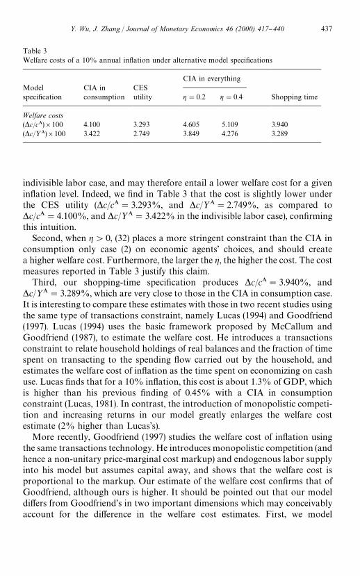
Table 3Welfare costs of a 10% annual in#ation under alternative model speci"cations

Modelspeci"cation

CIA inconsumption

CESutility

CIA in everything

g"0.2 g"0.4 Shopping time


indivisible labor case, and may therefore entail a lower welfare cost for a givenin#ation level. Indeed, we "nd in Table 3 that the cost is slightly lower underthe CES utility (*c/cA"3.293%, and *c/>A"2.749%, as compared to*c/cA"4.100%, and *c/>A"3.422% in the indivisible labor case), con"rmingthis intuition.

Second, when g'0, (32) places a more stringent constraint than the CIA inconsumption only case (2) on economic agents' choices, and should createa higher welfare cost. Furthermore, the larger the g, the higher the cost. The costmeasures reported in Table 3 justify this claim.

Third, our shopping-time speci"cation produces *c/cA"3.940%, and*c/>A"3.289%, which are very close to those in the CIA in consumption case.It is interesting to compare these estimates with those in two recent studies usingthe same type of transactions constraint, namely Lucas (1994) and Goodfriend(1997). Lucas (1994) uses the basic framework proposed by McCallum andGoodfriend (1987), to estimate the welfare cost. He introduces a transactionsconstraint to relate household holdings of real balances and the fraction of timespent on transacting to the spending #ow carried out by the household, andestimates the welfare cost of in#ation as the time spent on economizing on cashuse. Lucas "nds that for a 10% in#ation, this cost is about 1.3% of GDP, whichis higher than his previous "nding of 0.45% with a CIA in consumptionconstraint (Lucas, 1981). In contrast, the introduction of monopolistic competi-tion and increasing returns in our model greatly enlarges the welfare costestimate (2% higher than Lucas's).

More recently, Goodfriend (1997) studies the welfare cost of in#ation usingthe same transactions technology. He introduces monopolistic competition (andhence a non-unitary price-marginal cost markup) and endogenous labor supplyinto his model but assumes capital away, and shows that the welfare cost isproportional to the markup. Our estimate of the welfare cost con"rms that ofGoodfriend, although ours is higher. It should be pointed out that our modeldi!ers from Goodfriend's in two important dimensions which may conceivablyaccount for the di!erence in the welfare cost estimates. First, we model


monopolistic competition within the framework of Benhabib and Farmer (1994)and our production technology is subject to strong increasing returns to scale;and second we allow capital accumulation in our economy. The latter invokesfurther e!ects of in#ation through output on consumption.

Finally, notwithstanding the di!erences in model speci"cations, the welfarecost estimates for a 10% in#ation under our sunspot economy are in the sameorder of magnitude and are large, thereby suggesting that our results are quiterobust and general.

7. Concluding remarks

This paper has introduced new elements } monopolistic competition andincreasing returns to scale } into a standard RBC model with a cash-in-advanceconstraint to re-estimate the welfare costs of in#ation. Under such an alternativehypothesis, the model economy is capable of generating the observed aggregate#uctuations even when there are no shocks to the fundamentals. In particular,we demonstrate that this model matches the stylized U.S. business cycles facts aswell as two more standard models, which forms the basis for our reexaminationof the issue of interest. In such a paradigm, it is found that the welfare cost ofin#ation depends on the magnitudes of scale parameters as well as on the degreeof competition among "rms, and that the cost is considerably higher than that instandard monetary RBC models.

The modest or small estimated welfare costs of in#ation reported in theliterature are inconsistent with the fact that people attach to in#ation signi"-cantly. If these small welfare results were true, the policy implication would bethat in#ation should have never become a major social problem. However,people have shown a strong revealed preference for low rates of in#ation, bytheir willingness to incur large costs to achieve a lower rate. For example, in theUnited States in the 1970s, when the rate of in#ation was signi"cantly low bycomparison with many historical episodes in other countries, often a substantialmajority of respondents to the Gallop Poll, sometimes as large as 80%, namedin#ation as &the most important problem facing the country' (see the analysis byFischer and Huizinga, 1982). To unravel this, we have explored the e!ects ofin#ation in a monopolistically competitive economy and obtained larger welfareresults than those documented in existing studies.

It should also be pointed out that in our model the indeterminacy of equili-bria arises from the shocks to agents' belief. This is consistent with the existingframework in monetary economics (e.g., see Farmer, 1995, Chapter 9). More-over, our exercise enriches the literature, in that we have not only proposeda monetary model in which sunspots matter, but also demonstrated that thiseconomy displays similar characteristics of business #uctuations to the actualU.S. economy.


14We are indebted to Dean Corbae for this suggestion.

Conceivably, there are two potential extensions. One approach is to endogen-ize each "rm's price markups over costs.14 Although we have experimented withvarying markups in our simulations and welfare computations, there still lacksan endogenous mechanism. Since many economists believe that cyclical vari-ations in markups are an important feature of business cycles (e.g., Rotembergand Woodford, 1991), it would be interesting to explore the implications ofendogenous markups in our context of monopolistic competition and increasingreturns to scale. A second approach is to incorporate either costless credit (e.g.,Cooley and Hansen, 1991) or costly credit (e.g., Gillman, 1993). These extensionsshould enable us to understand better the e!ects of in#ation in alternativeeconomies.

References

Baxter, M., King, R.G., 1991. Productive externalities and business cycles. Discussion Paper 53,Institute for Empirical Macroeconomics, Federal Reserve Bank of Minneapolis.

Benhabib, J., Farmer, R.E.A., 1994. Indeterminacy and increasing returns. Journal of EconomicTheory 63, 19}41.

Caballero, R.J., Lyons, R.K., 1992. External e!ects in U.S. procyclical productivity. Journal ofMonetary Economics 29, 209}226.

Cooley, T.F., Hansen, G.D., 1989. The in#ation tax in a real business cycle model. AmericanEconomic Review 79, 733}748.

Cooley, T.F., Hansen, G.D., 1991. The welfare cost of moderate in#ation. Journal of Money, Credit,and Banking 23, 482}503.

Den Haan, W.J., 1990. The optimal in#ation path in a Sidrauski-type model with uncertainty.Journal of Monetary Economics 25, 389}410.

Domowitz, I.R., Hubbard, G., Petersen, B.C., 1988. Market structure and cyclical #uctuations inU.S. manufacturing. Review of Economics and Statistics 70, 55}66.

Farmer, R.E.A., 1995. The Macroeconomics of Self-Ful"lling Prophecies. MIT Press, Cambridge,MA.

Farmer, R.E.A., Guo, J.-T., 1994. Real business cycles and the animal spirits hypothesis. Journal ofEconomic Theory 63, 42}72.

Fischer, S., 1981. Towards an understanding of the costs of in#ation: II. Carnegie-RochesterConference Series on Public Policy 15, 5}41.

Fischer, S., Huizinga, J., 1982. In#ation, unemployment and public opinion polls. Journal of Money,Credit, and Banking 14, 1}19.

Gillman, M., 1993. The welfare costs of in#ation in a cash-in-advance economy with costly credit.Journal of Monetary Economics 31, 97}115.

Gomme, P., 1993. Money and growth revisited: measuring the costs of in#ation in an endogenousgrowth model. Journal of Monetary Economics 32, 51}77.

Goodfriend, M., 1997. A framework for the analysis of moderate in#ations. Journal of MonetaryEconomics 39, 45}65.

Hall, R.E., 1986. Market structure and macroeconomic #uctuations. Brookings Papers on EconomicActivity 2, 285}322.


Hall, R.E., 1988. The relation between price and marginal cost in U.S. industry. Journal of PoliticalEconomy 96, 921}947.

Hall, R.E., 1990. Invariance properties of Solow's productivity residual. In: Diamond, P. (Ed.),Growth-Productivity-Unemployment. MIT Press, Cambridge, MA.

Hansen, G.D., 1985. Indivisible labor and the business cycle. Journal of Monetary Economics 16,309}328.

Hornstein, A., 1993. Monopolistic competition, increasing returns to scale, and the importance ofproductivity shocks. Journal of Monetary Economics 31, 299}316.

Kydland, F.E., Prescott, E., 1982. Time to build and aggregate #uctuations. Econometrica 50,1345}1370.

Lucas Jr., R.E., 1980. Equilibrium in a pure currency economy. In: Karaken, J.H., Wallace, N. (Eds.),Models of Monetary Economies. Federal Reserve Bank, Minneapolis, MN.

Lucas Jr., R.E., 1981. Discussion of: Stanley Fischer, &Towards an understanding of the costs ofin#ation: II'. Carnegie-Rochester Conference Series on Public Policy 15, 43}52.

Lucas Jr., R.E., 1984. Money in a theory of "nance. Carnegie-Rochester Conference Series on PublicPolicy 21, 9}46.

Lucas Jr., R.E., 1988. On the mechanism of economic development. Journal of Monetary Economics22, 3}42.

Lucas Jr., R.E., 1994. On the welfare cost of in#ation. Mimeo, University of Chicago.Lucas Jr., R.E., Stokey, N.L., 1983. Optimal "scal and monetary policy in an economy without

capital. Journal of Monetary Economics 12, 55}93.Lucas Jr., R.E., Stokey, N.L., 1987. Money and interest in a cash-in-advance economy. Econo-

metrica 55, 491}514.McCallum, B.T., Goodfriend, M., 1987. Demand for money: theoretical studies. In: Eatwell, J.,

Milgate, M., Newman, P. (Eds.), The New Palgrave: A Dictionary of Economics. Stockton Press,London; Macmillan, New York, pp. 775}781.

Rogerson, R., 1988. Indivisible labor, lotteries and equilibrium. Journal of Monetary Economics 21,3}16.

Rotemberg, J.J., Woodford, M., 1991. Markups and the business cycle. NBER MacroeconomicsAnnual 6, 63}128.

Wu, Y., Zhang, J., 1998. Endogenous growth and the welfare costs of in#ation. Journal of EconomicDynamics and Control 22, 465}482.


Documents

Monopolistic competition, increasing returns to scale, and the