Chemical tuning of the magnetic relaxation in Dysprosium(III) mononuclear complexes

Luke J. Batchelor,a Irene Cimatti,a Régis Guillot,a Floriana Tuna,b Wolfgang Wernsdorfer,c Liviu Ungur,d, Liviu F. Chibotaru,d Victoria E. Campbell,a and Talal Mallah*a

a Institut de Chimie Moléculaire et des Matériaux d’Orsay, Université Paris-Sud, 91405 Orsay Cedex, France. E-mail: talal.mallah@u-psud.fr b EPSRC National UK EPR Facility, School of Chemistry and Photon Science Institute, The University of Manchester, Oxford Road, Manchester, M13 9PL, UK.c Laboratoire Louis Néel, CNRS, 25 Avenue des Martyrs BP 166, 38042 Grenoble Cedex 9, France.d Theory of Nanomaterials Group and INPAC—Institute of Nano- scale Physics and Chemistry, Katholieke Universiteit Leuven Celestijnenlaan 200F, 3001 Heverlee , Belgium.

Experimental SectionGeneral Procedures. Unless otherwise stated, all reagents were purchased from Aldrich or TCI and used without further purification. H2DABPH was synthesized according to literature procedures.1 All manipulations were conducted under standard bench top conditions. Infrared (IR) data were measured on KBr pellets using a PerkinElmer FTIR spectrometer. Electrospray ionization mass spectrometry (ESI-MS) spectra were recorded on a Thermo Scientific 2009 mass spectrometer. NMR spectra were recorded on a Bruker Aspect 300 NMR spectrometer. Elemental analysis was taken on a Thermo Scientific Flash analyzer.Magnetic Measurements. The magnetic susceptibility measurements were obtained using a Quantum Design SQUID MPMS-XL7 magnetometer operating between 1.8 and 300 K for direct-current (dc) applied fields ranging from -7 to +7 T. dc analysis was performed on polycrystalline samples of 1 and 2 wrapped in eicosan under a field between 0.1 and 1 T and between 1.8 and 300 K. Alternating-current (ac) susceptibility measurements were carried out under an oscillating field of 1.5 or 3 Oe and ac frequencies ranging between 0.1 and 1500 Hz. Data were corrected for the diamagnetism of the compounds (Pascal constants) and the sample holder and eicosane matrix. Single-Crystal X-ray Diffraction Studies. X-ray diffraction data were collected by using a Bruker Kappa X8 APEX II diffractometer with graphite-monochromated Mo K radiation (= 0.71073 Å). Crystals were mounted on a CryoLoop (Hampton Research) with paratone-N (Hampton Research) as the cryoprotectant and then flash frozen in a nitrogen-gas stream at 100 K. The temperature of the crystal was maintained at the selected value (100 K) by means of a Cryostream 700 series cooling device to within an accuracy of ±1 K. The data were corrected for Lorentz polarization and absorption effects. The structures were solved by direct methods using SHELXS- 972 and refined against F2 by full-matrix least-squares techniques using SHELXL-973 with anisotropic displacement parameters for all non-hydrogen atoms. Hydrogen atoms were located on a difference Fourier map and introduced into the calculations as a riding model with isotropic thermal parameters. All calculations were performed using the Crystal Structure crystallographic software package WINGX.4

The crystal data collection and refinement parameters are given in Table S1 and selected bond lengths are given in Table S2.CCDC 870723 and 870724, contain the supplementary crystallographic data for this paper. These data can be obtained free of charge from the Cambridge Crystallographic Data Centre via www.ccdc.cam.ac.uk/data_ request/cif.

1

Electronic Supplementary Material (ESI) for Dalton Transactions.This journal is © The Royal Society of Chemistry 2014

Table S1. Crystallographic data for 1 and 2. Compound 1 2Formula C46H47N13DyO15.5

, C48H55N12DyO15

fw 1192.47 1202.54Crystal size / mm3 0.05 x 0.08 x 0.09 0.26 x 0.24 x 0.11Crystal system triclinic triclinicSpace group P -1 P -1a, Å 11.9478(9) 11.507(4)b, Å 12.4520(9) 12.912(5)c, Å 18.3958(12) 17.853(5)α, ° 95.818(2) 97.274(4)β, ° 102.994(2) 100.839(5)γ, ° 108.904(2) 102.255(5),Cell volume, Å3 2477.4(3) 2507.3(15)Z 2 2T, K 100(1) 100(1)F000 1208 1226µ / mm–1 1.592 1.593 range / ° 1.76 – 36.34 1.86 – 43.41Refl. collected 40 295 85 656Refl. unique 18 317 22 076Rint 0.0389 0.0146GOF 1.089 1.120Refl. obs. (I>2(I)) 15 696 21 154Parameters 732 682wR2 (all data) 0.1558 0.0560R value (I>2(I)) 0.0569 0.0212Largest diff. peak and hole (e-.Å-3)

-1.301 ; 1.741 -1.675 ; 1.584

Table S2 Selected bond distances. 1 2

Dy-N2 2.554(3) Å Dy-N2 2.5057(10) Å

Dy-N3 2.672(3) Å Dy-N3 2.6402(12) Å

Dy-N4 2.555(3) Å Dy-N4 2.5697(11) Å

Dy-N7 2.567(3) Å Dy-N7 2.5349(15 Å

Dy-N8 2.647(3) Å Dy-N8 2.6699(11) Å

Dy-N9 2.556(3) Å Dy-N9 2.5320(12) Å

Dy-O1 2.404(3) Å Dy-O1 2.3185(8) Å

Dy-O2 2.414(3) Å Dy-O2 2.5094(10) Å

Dy-O3 2.395(3) Å Dy-O3 2.4126(11) Å

Dy-O4 2.420(3) Å Dy-O4 2.4880(12) Å

2

Synthesis. Synthesis of [Dy(H2DABPH)2](NO3)3∙2.5H2O (1) H2DABPH (0.125 g, 0.31 mmol) was suspended in EtOH (96%, 6 mL) and the temperature raised to 55 °C. Dy(NO3)3∙5H2O (0.068 g, 0.16 mmol) dissolved in EtOH (96%, 6 mL) was added dropwise with stirring, forming an intense yellow mixture that was stirred for 30 minutes at 55 °C. This was then filtered and left to slowly evaporate yielding a yellow powder after several days (0.065 g, 34%). Crystals suitable for X-ray diffraction were grown by slow diffusion of Et2O into an aliquot of the yellow solution obtained upon filtration. Elemental analysis (%), observed (calculated for DyC46H47N13O15.5) C, 45.91 (46.26) H, 4.02 (3.96) N, 15.23 (15.26). MS ESI+ (MeOH): m/z 960.25 [Dy(HDABPH)2]+. IR (KBr) ν/cm-1: 3411 (s), 3069 (m), 2919 (w), 2769 (w), 2426 (w), 1767 (w), 1602 (s), 1568 (s), 1547 (m), 1528 (m), 1487 (m), 1384 (s), 1316 (s), 1264 (m), 1202 (w), 1188 (w), 1158 (m), 1124 (w), 1101 (w), 1074 (m), 1026 (w), 1004 (w), 917 (w), 897 (w), 815 (m), 804 (w), 744 (w), 715 (s), 691 (m), 558 (w), 523 (w), 466 (w), 421 (w).Synthesis of [Dy(H2DABPH)(HDABPH)](NO3)2∙EtOH∙4H2O (2) H2DABPH (0.125 g, 0.31 mmol) was suspended in H2O (6 ml) and the temperature raised to 55 °C. Dy(NO3)3∙5H2O (0.068 g, 0.16 mmol) dissolved in EtOH (96%, 6 ml) was added dropwise with stirring, forming an intense yellow mixture that was stirred for 30 minutes at 55 °C. This was then filtered and left to slowly evaporate yielding large X-ray quality crystals in low yield after several weeks. Elemental analysis (%), observed (calculated for DyC48H55N12O15) C, 47.82 (47.87) H, 4.34 (4.61) N, 14.10 (13.96). MS ESI+ (MeOH): m/z 960.25 [Dy(HDABPH)2]+. IR (KBr) ν/cm-1: 3420 (s), 3071 (m), 2919 (w), 2767 (w), 2426 (w), 1767 (w), 1602 (s), 1568 (s), 1547 (m), 1528 (m), 1488 (m), 1384 (s), 1316 (s), 1264 (m), 1203 (w), 1188 (w), 1159 (m), 1124 (w), 1101 (w), 1075 (m), 1027 (w), 1004 (w), 918 (w), 898 (w), 815 (m), 745 (w), 715 (s), 691 (m), 557 (w), 524 (w), 466 (w), 421 (w).

Figure S1. Electrospray mass spectrum of 1. Close up of molecular peak (red) with simulated Isotope pattern (black), inset.

Figure S2. Frequency of χ’ (dotted lines) and χ” (solid lines) of 1 (left) and 2 (right) under 1000 Oe applied dc field, in an ac field of 1.55 G oscillating at frequencies from 2 to 6 K.

3

Figure S3. χT vs.T for 1 at 0.1 and 1.0 T overlaid, and M vs. H/T (inset) collected at 2, 4 and 6 K.

Figure S4. χT vs.T for 2 at 0.1 and 1.0 T overlaid, and M vs. H/T (inset) collected at 2, 4 and 6 K.

4

Figure S5. Hysteresis loops of 1.

Figure S6. Hysteresis loops of 1.

5

Ab initio calculations

Computational details

All calculations were done with MOLCAS 7.6 and 7.8 and are of CASSCF / RASSI / SINGLE_ANISO type.We have employed 2 structural approximations (A – a reduced fragment of the molecule and B – the entire molecule) and 2 basis set approximations (1 –small and 2-large), resulting in 4 computational approximations for each molecule (A1, A2, B1 and B2)

Figure S7. Structure of the fragment A.

Table S3. Contractions of the employed basis sets in computational approximations 1 and 2.Basis 1 Basis 2

Dy.ANO-RCC...7s6p4d3f1g.O.ANO-RCC...3s2p1d.N.ANO-RCC...3s2p1d. (close)N.ANO-RCC...3s2p. (distant)C.ANO-RCC...3s2p. H.ANO-RCC...2s.

Dy.ANO-RCC...8s7p5d4f2g1h. O.ANO-RCC...4s3p2d. N.ANO-RCC...4s3p2d. C.ANO-RCC...4s3p2d. (close)C.ANO-RCC...4s3p. (distant)H.ANO-RCC...3s1p. (close)H.ANO-RCC...2s. (distant)

In order to check the influence of the crystal environment we have performed embedded cluster calculations for both molecules. We have built three cluster models.

model 1: -- all neighboring molecules were considered as point charges:+2 for the Dy ion and -1 for the NO3- ion.

model 2: -- the closest molecules of water and NO3 ions were considered in the ab initio calculation (with electrons and basis sets), while the other ions were considered as point charges:+2 for the Dy ion and -1 for the NO3

- ion. model 3 – the same as model 2, the difference being that now more NO3

- ions and water molecules are considered in the ab initio calculation.

In all cluster models the number of point charges was very large (64000 pc for 1 and 48000 pc for 2).

6

Electronic and magnetic properties of the complex (1)Table S4. Energies of the lowest spin-free states and of the lowest Kramers doublets.

A1 A2 B1 B2 B1_1 B1_2 B1_3 B2_1individual molecule molecule embedded in a model cluster

0.00095.690

105.841129.015147.574207.574312.156475.794

3594.281 3644.089 3651.645 3688.779 3731.042 3793.639 3907.658 6115.463 6140.928 6184.849 6262.614 6304.583 6383.863 8060.067 8092.167 8168.622 8254.391 8329.378 9569.206 9632.804 9753.328 9846.740

…

0.00064.26086.449

101.357147.846184.127282.633439.944

3593.540 3619.208 3627.679 3666.387 3711.806 3767.228 3870.889 6102.997 6120.736 6162.743 6241.205 6280.910 6346.813 8038.702 8076.056 8146.217 8233.431 8292.987 9545.467 9620.053 9731.175 9811.668

…

0.00052.14876.82694.186

158.106182.856275.652432.126

3596.503 3612.586 3623.119 3662.692 3711.193 3765.095 3863.095 6096.629 6122.643 6159.434 6240.350 6281.956 6339.605 8033.032 8075.296 8145.373 8236.393 8287.556 9538.623 9622.314 9732.718 9806.245

…

0.000 24.797 56.448 79.022147.235179.535253.169404.120

3581.0633595.5923615.0163645.5693695.8693747.1853834.5946076.9926114.8256143.1866222.7416265.1856310.7058013.5348063.8798129.1578219.8808258.9489518.9659613.3359715.0519778.551

…

0.00069.04097.978

127.255159.271203.950292.658440.879

3600.6363618.7523656.3673683.8843726.2863776.5833876.1646109.8446136.4096180.7466254.1666292.4366356.5148050.1998089.9968159.7148247.2118305.2219558.0479632.5689745.4299823.585

…

0.00059.49795.391

123.290162.152200.983286.708429.704

3599.7383613.1143655.7673681.0833723.2643770.3273866.0586106.4466133.9256178.9946250.6786287.4266347.4948046.0128087.9758156.6008243.5688297.1119553.4209631.8109741.7789815.695

…

0.00050.74093.998

126.339161.258198.309285.790429.073

3596.5693613.0263651.9733680.1703722.2423768.8123865.8556104.5436132.5996176.6526248.7956285.6796347.5068044.1608086.4428154.6768241.8368296.5059551.3459630.9879738.8129815.521

…

0.00044.58683.810

100.261158.605185.944268.356412.986

3595.1543603.5983636.3993663.9653708.1863756.8673847.0516094.9456124.2196161.4096234.5756274.3566326.5998031.6168076.6248140.8288229.4268275.6419538.1779621.2169726.6849794.771

…

Table S5. g tensors of the lowest Kramers doublets (KD) for the individual molecule.A1 A2 B1 B2KD

E (cm-1) g E (cm-1) g E (cm-1) g E (cm-1) g1 gX

gYgZ

0.000 0.0261 0.045517.1586

0.000 0.0320 0.080117.0842

0.000 0.0558 0.161016.9165

0.000 0.1552 0.240116.5915

2 gXgYgZ

95.690 1.0880 3.219610.9030

64.260 0.2989 2.054116.5405

52.148 0.6101 1.842517.0240

24.797 0.5809 1.575117.1328

3 gXgYgZ

105.841 0.5045 2.296111.2809

86.449 0.58944.12819.8645

76.826 9.34325.67080.3386

56.448 0.1691 1.988213.1928

4 gXgYgZ

129.015 9.63455.84680.7077

101.357 1.76481.98849.6075

94.186 2.49393.07308.3555

79.022 0.5955 2.316211.3615

5 gXgYgZ

147.574 0.9417 4.448811.6734

147.846 0.4990 0.740816.7904

158.106 1.0559 3.485411.3782

147.235 7.61996.49894.6269

6 gXgYgZ

207.574 7.58756.87066.0450

184.127 5.72206.38267.4268

182.856 2.32983.66609.6999

179.535 0.4281 0.919615.6143

7 gXgYgZ

312.156 0.7786 0.938215.4003

282.633 0.5864 0.698515.3479

275.652 0.6207 0.851915.1503

253.169 0.4636 0.986914.9004

8 gXgYgZ

475.794 0.1407 0.194319.2271

439.944 0.1289 0.206319.1926

432.126 0.1347 0.226019.1586

404.120 0.1216 0.235319.1266

7

Table S6. g tensors of the lowest Kramers doublets (KD) for the molecule embedded in a model cluster.B1_1 B1_2 B1_3 B2_1KD

E (cm-1) g E (cm-1) g E (cm-1) g E (cm-1) g1 gX

gYgZ

0.000 0.0929 0.173317.3633

0.000 0.1742 0.260617.3310

0.000 0.2325 0.365717.2032

0.000 0.1738 0.335617.1879

2 gXgYgZ

69.040 0.8315 1.171517.1454

59.497 0.9362 1.071117.3862

50.740 0.6342 0.859517.8723

44.586 0.5108 1.065717.7456

3 gXgYgZ

97.978 0.1613 2.879012.0883

95.391 0.1064 2.695212.1860

93.998 0.0554 1.860212.5579

83.810 1.3915 4.794111.6991

4 gXgYgZ

127.255 0.8175 2.146014.5883

123.290 0.9646 2.082114.9305

126.339 0.5973 1.888615.9917

100.261 2.2382 4.138510.0491

5 gXgYgZ

159.271 0.3369 0.599516.6703

162.152 0.1339 0.940016.5844

161.258 0.0576 1.034016.1070

158.605 0.7986 1.348014.6660

6 gXgYgZ

203.950 5.47545.73506.9402

200.983 4.89935.58866.4183

198.309 4.55085.51276.7377

185.944 3.80654.80867.4643

7 gXgYgZ

292.658 1.2039 2.032014.6133

286.708 1.3207 2.353714.3241

285.790 1.2280 2.106414.5065

268.356 1.1284 1.927314.5304

8 gXgYgZ

440.879 0.1733 0.281519.1063

429.704 0.1874 0.318319.0604

429.073 0.1847 0.309819.0633

412.986 0.1608 0.285219.0897

Table S7. Angles between the main magnetic axes of the lowest Kramers doublet obtained in different computational approximations (degrees)

A1 A2 B1 B2 B1_1 B1_2 B1_3 B2_1A1 0.000 0.508 1.313 3.135 11.701 14.028 13.543 10.996A2 0.508 0.000 0.805 2.646 12.190 14.463 13.947 11.488B1 1.313 0.805 0.000 1.890 12.969 15.160 14.599 12.270B2 3.135 2.646 1.890 0.000 14.835 17.042 16.458 14.131

B1_1 11.701 12.190 12.969 14.835 0.000 4.204 5.132 0.740B1_2 14.028 14.463 15.160 17.042 4.204 0.000 1.571 4.737B1_3 13.543 13.947 14.599 16.458 5.132 1.571 0.000 5.508B2_1 10.996 11.488 12.270 14.131 0.740 4.737 5.508 0.000

Figure S8. Orientation of the main anisotropy axis of the ground Kramers doublet of 1.

8

0 50 100 150 200 250 3008

9

10

11

12

13

14

experiment H=0.1 T experiment H=1.0 T model A1 model A2 model B1 model B2 cluster B1_1 cluster B1_2 cluster B1_3 cluster B2_1T

(em

u K

mol

-1)

T (K)Figure S9. A comparison between measured and calculated magnetic susceptibility of 1.

0.0 0.5 1.0 1.5 2.0 2.5 3.0 3.5 4.0 4.5 5.0 5.50.00.51.01.52.02.53.03.54.04.55.05.5

T = 2.0 K Experiment model A1 model A2 model B1 model B2 cluster B1_1 cluster B1_2 cluster B1_3 cluster B2_1

M / B

H / TFigure S10. Measured and calculated molar magnetization of 1 at 2.0 K.

9

0.0 0.5 1.0 1.5 2.0 2.5 3.0 3.5 4.0 4.5 5.0 5.50.00.51.01.52.02.53.03.54.04.55.05.5

T = 4.0 K Experiment model A1 model A2 model B1 model B2 cluster B1_1 cluster B1_2 cluster B1_3 cluster B2_1

M / B

H / TFigure S11. Measured and calculated molar magnetization of 1 at 4.0 K.

0.0 0.5 1.0 1.5 2.0 2.5 3.0 3.5 4.0 4.5 5.0 5.50.00.51.01.52.02.53.03.54.04.55.05.5

T = 6.0 K Experiment model A1 model A2 model B1 model B2 cluster B1_1 cluster B1_2 cluster B1_3 cluster B2_1

M / B

H / TFigure S12. Measured and calculated molar magnetization of 1 at 6.0 K.

10

Analysis of the multiplet-specific crystal-field for compound 1.

Recently, the extraction of the parameters of the multiplet-specific crystal-field for lanthanides methodology has been implemented in the SINGLE_ANISO program in MOLCAS. The results presented below use the ab initio CASSCF/RASSI wave function and energies to compute the parameters of the crystal-field splitting of the ground J multiplet.

The Crystal-Field Hamiltonian:𝐻𝐶𝐹=∑

𝑘,𝑞

𝐵𝑞𝑘𝑂𝑞𝑘

where:

-- Extended Stevens Operators (ESO)as defined in:𝑂𝑞𝑘 1. Rudowicz, C.; J. Phys. C: Solid State Phys.,18 (1985) 1415-1430. 2. Implemented in the "EasySpin" function in MATLAB, www.easyspin.org. - the rank of the ITO, = 2, 4, 6.𝑘 - the component (projection) of the ITO, = , , ... , , ... ;𝑞 ‒ 𝑘 ‒ 𝑘+ 1 0 1 𝑘

Quantization axis was chosen the main magnetic axis of the ground Kramers doublet (pseudospin s=1/2).

Table S8. Parameters of the effective Crystal Field acting on the ground J=15/2 multiplet..

N M A1 A2 B1 B22 -2 -0.1410989E+01 -0.4130607E+00 -0.3634647E+00 -0.6512456E+002 -1 -0.4328904E-01 0.1106928E+00 0.6936372E-01 0.1007530E+002 0 -0.1035036E+01 -0.7461816E+00 -0.5889409E+00 -0.3653693E+002 1 -0.4568591E+00 0.2773090E+00 0.1826040E+00 -0.8139541E-012 2 0.2150954E+01 0.2487760E+01 0.2536468E+01 0.2424200E+014 -4 -0.2714479E-01 -0.1184939E-01 -0.1013485E-01 -0.1749135E-014 -3 0.2255613E-02 0.4898691E-02 0.5305023E-02 -0.1010485E-024 -2 0.5497318E-02 0.2719492E-02 0.2592268E-02 0.3361123E-024 -1 -0.4325094E-03 -0.4910263E-04 -0.5777652E-04 -0.4309213E-034 0 0.2595787E-03 0.2114033E-03 0.4965086E-03 0.4692646E-034 1 0.2705348E-02 -0.2439925E-02 -0.2875732E-02 0.2650939E-024 2 -0.5611770E-02 -0.7171700E-02 -0.7506559E-02 -0.6836210E-024 3 -0.1259204E-01 0.1129162E-01 0.1011421E-01 -0.1079945E-014 4 0.9663426E-02 0.2755547E-01 0.2774037E-01 0.2513642E-016 -6 -0.9681365E-04 -0.4409628E-04 -0.3916625E-04 -0.6825432E-046 -5 0.2966491E-03 -0.1418384E-03 -0.1022291E-03 0.1121241E-036 -4 0.2173661E-03 0.6967634E-04 0.6230836E-04 0.1120626E-036 -3 -0.1393358E-03 0.1168955E-03 0.1343446E-03 -0.1774737E-036 -2 0.4944217E-04 0.4212918E-04 0.5308580E-04 0.8374830E-046 -1 -0.4343741E-04 -0.3945252E-04 -0.7872007E-04 0.1318973E-036 0 0.6200942E-04 0.6082844E-04 0.6247906E-04 0.5873687E-046 1 0.3049450E-03 -0.2928675E-03 -0.2869256E-03 0.2940102E-036 2 -0.2205799E-04 -0.4031740E-04 -0.4639259E-04 -0.3433881E-046 3 0.6765839E-05 -0.7465818E-04 -0.7336487E-04 0.1924207E-046 4 -0.1041330E-03 -0.2213253E-03 -0.2382416E-03 -0.2005645E-036 5 0.1708513E-04 0.2330511E-03 0.2490888E-03 -0.2462006E-036 6 -0.1492695E-04 0.8058785E-04 0.8724809E-04 0.6051560E-04

N M B1_1 B1_2 B1_3 B2_12 -2 -0.1163448E+00 -0.9365532E+00 -0.1433209E+01 -0.8702039E+002 -1 -0.1106466E+01 -0.1295209E+01 -0.1180015E+01 -0.1205887E+012 0 -0.9124152E+00 -0.8767283E+00 -0.8432189E+00 -0.6798181E+002 1 0.2542564E+00 -0.2447607E+00 -0.4675687E+00 -0.8472623E-012 2 0.2230105E+01 0.1923202E+01 0.1691702E+01 0.2020954E+014 -4 -0.1536462E-01 -0.2723652E-01 -0.2465973E-01 -0.2699405E-014 -3 -0.1875331E-01 -0.9582094E-02 0.1477327E-02 -0.1902644E-01

11

4 -2 0.1021499E-02 0.5358861E-02 0.7345133E-02 0.3380133E-024 -1 0.3783298E-02 0.3978350E-02 0.3381627E-02 0.4187144E-024 0 0.6376763E-03 0.8649822E-03 0.8512013E-03 0.5868922E-034 1 -0.3577497E-02 -0.5871427E-03 0.8670686E-03 -0.2838041E-024 2 -0.8114130E-02 -0.6788829E-02 -0.4510898E-02 -0.7186783E-024 3 0.3483795E-02 -0.1483992E-01 -0.1701589E-01 -0.5026846E-024 4 0.2284232E-01 0.3742586E-02 -0.1255066E-01 0.9386061E-026 -6 -0.1298276E-03 -0.1072878E-03 0.1000310E-04 -0.9869787E-046 -5 0.1413985E-03 -0.2981009E-03 -0.5793420E-03 -0.3639634E-036 -4 0.1293285E-03 0.1752456E-03 0.1505424E-03 0.1892500E-036 -3 0.1751685E-03 0.1151393E-03 -0.1002779E-04 0.1140781E-036 -2 0.1785658E-03 0.1664862E-03 0.1550075E-03 0.1719848E-036 -1 -0.3068621E-03 -0.3574563E-03 -0.3292405E-03 -0.2210773E-036 0 0.4126525E-04 0.4044196E-04 0.4469959E-04 0.4221682E-046 1 -0.3431708E-03 -0.2673314E-03 -0.2664184E-03 -0.3880152E-036 2 -0.5029206E-04 -0.6317698E-04 -0.4162912E-04 0.1199885E-046 3 0.7283953E-04 0.2655582E-03 0.2700636E-03 0.1171625E-036 4 -0.1420079E-03 0.2643625E-05 0.1130634E-03 -0.3406110E-046 5 0.6417161E-03 0.5934657E-03 0.2779913E-03 0.5081089E-036 6 0.4031346E-04 -0.1063185E-03 -0.1459958E-03 -0.7841626E-04

Recovery factor of the initial energy matrix using the above parameters for each computational model:model Recovery factorA1 98.060289 %A2 98.057936 %B1 97.991083 %B2 97.789334 %B1_1 96.694771 %B1_2 96.717495 %B1_3 96.841595 %B2_1 96.671641 %

The rest of the energy matrix is accounted by the higher-rank operators (n=8, 10, … , 14).

12

Electronic and magnetic properties of the complex (2)

Table S9. Energies of the lowest spin-free states and of the lowest Kramers doublets.A1 A2 B1 B2 B1_1 B1_2 B2_1

individual molecule molecule embedded in a model cluster 0.000 66.028

159.786 222.006 259.290 309.964 410.610 535.825 3590.085 3668.767 3714.719 3776.255 3831.120 3866.320 3986.540 6138.962 6189.991 6254.634 6325.115 6371.915 6473.005 8096.280 8154.987 8229.965 8317.381 8408.394 9607.956 9713.886 9799.990 9927.611

…

0.000 72.371 162.601 228.464 262.499 295.908 391.031 507.248 3590.973 3676.786 3711.968 3770.964 3825.411 3852.669 3957.869 6140.148 6191.952 6248.947 6314.419 6365.149 6447.407 8095.426 8151.510 8223.352 8309.766 8385.225 9604.611 9713.405 9791.213 9906.257

…

0.000 68.662 155.704 221.481 259.563 285.076 379.728 498.433 3590.285 3675.916 3708.989 3764.976 3817.852 3845.332 3947.661 6137.795 6189.163 6245.057 6310.892 6362.655 6437.061 8091.809 8146.835 8221.839 8309.066 8377.438 9599.356 9711.098 9791.103 9898.470

…

0.000 79.388160.085219.937262.477287.923366.841477.074

3592.9773679.1853714.5183763.1743812.5903840.5963926.2996139.6076192.9006243.5186304.4796360.1686418.2828092.0038146.3008219.8728304.4708361.0899597.9189713.7829785.7369883.329

…

0.00040.347

122.806181.529211.942239.137327.690443.574

3579.4783643.1133684.6053726.5923768.7673795.8583890.2596116.7086156.1366215.7046271.7166317.5476380.3458063.9858115.3038184.4338268.9168326.6729572.6049667.7689761.0539846.914

…

0.00047.995

125.497174.337205.383242.863322.612434.232

3582.1093638.6203692.1973728.1073762.1563794.0293879.0416116.3326155.3956220.1986269.5296316.8446369.1608063.8518115.3778183.9558268.2828318.7489574.3249662.7959765.2749838.511

…

0.00044.075

125.206177.649217.537237.683316.033423.099

3579.0473651.5833680.6093722.1923763.1703790.9653869.9316116.4926158.8556210.9116263.5876314.2536362.2718061.8948113.8248179.7778263.4448310.4679568.5939669.6229753.8299831.862

…

Table S10. g tensors of the lowest Kramers doublets (KD).A1 A2 B1 B2KD

E (cm-1) g E (cm-1) g E (cm-1) g E (cm-1) g1 gX

gYgZ

0.000 0.1660 0.425418.8633

0.000 0.1431 0.328119.2104

0.000 0.1657 0.371719.2138

0.000 0.1298 0.256919.4618

2 gXgYgZ

66.028 0.4920 0.678915.0109

72.371 0.5721 0.695515.6027

68.662 0.5092 0.704815.6152

79.388 0.6489 0.753216.1261

3 gXgYgZ

159.786 0.8384 1.746112.7002

162.601 1.1731 2.171512.4542

155.704 0.7898 1.834912.2454

160.085 1.0485 2.230112.1399

4 gXgYgZ

222.006 0.3362 1.204314.1237

228.464 0.2138 2.033912.0301

221.481 1.3221 2.298812.0868

219.937 1.0898 2.650312.8101

5 gXgYgZ

259.290 3.38415.29289.1673

262.499 2.7373 5.085411.9320

259.563 10.7733 6.2718 1.3356

262.477 0.4010 3.369010.7756

6 gXgYgZ

309.964 2.0778 2.162914.3136

295.908 1.3018 1.528313.5168

285.076 0.3066 2.653310.9892

287.923 2.0779 4.313612.3749

7 gXgYgZ

410.610 0.8662 1.205615.9723

391.031 0.9564 1.326715.6192

379.728 0.9843 1.396815.4301

366.841 1.0549 1.619414.9353

8 gXgYgZ

535.825 0.1805 0.370618.9371

507.248 0.2003 0.432818.8245

498.433 0.2052 0.442518.8164

477.074 0.2273 0.517518.7063

13

Table S11. g tensors of the lowest Kramers doublets (KD).B1_1 B1_2 B2_1KD

E (cm-1) g E (cm-1) g E (cm-1) g1 gX

gYgZ

0.000 0.2690 0.821418.0930

0.000 0.2145 0.547518.1891

0.000 0.2480 0.649418.7799

2 gXgYgZ

40.347 0.1680 0.906114.4821

47.995 0.4568 0.878215.4900

44.075 0.2528 0.840415.0701

3 gXgYgZ

122.806 0.3508 1.263412.5127

125.497 0.2645 1.222412.4643

125.206 0.5487 1.546112.4646

4 gXgYgZ

181.529 0.6872 2.813213.4578

174.337 0.4310 2.999014.2808

177.649 0.4931 1.964615.2743

5 gXgYgZ

211.942 1.8706 3.036411.8783

205.383 0.4619 2.527412.8596

217.537 2.35784.84258.9502

6 gXgYgZ

239.137 2.52423.84908.1912

242.863 2.90424.57757.1087

237.683 1.38782.35589.9854

7 gXgYgZ

327.690 1.5984 2.755614.1260

322.612 2.1233 4.397912.7207

316.033 1.7048 2.908913.7091

8 gXgYgZ

443.574 0.2738 0.588918.7323

434.232 0.3225 0.731818.6455

423.099 0.3005 0.684518.6142

Table S12. Angles between the main magnetic axes of the lowest Kramers doublet obtained in different computational approximations (degrees)

A1 A2 B1 B2 B1_1 B1_2 B2_1A1 0.000 8.288 9.434 14.215 8.457 22.385 6.377A2 8.288 0.000 1.342 5.929 16.604 30.445 2.171B1 9.434 1.342 0.000 4.838 17.819 31.693 3.503B2 14.215 5.929 4.838 0.000 22.513 36.303 7.978B1_1 8.457 16.604 17.819 22.513 0.000 13.929 14.541B1_2 22.385 30.445 31.693 36.303 13.929 0.000 28.332B2_1 6.377 2.171 3.503 7.978 14.541 28.332 0.000

Figure S13. Orientation of the main anisotropy axis of the ground Kramers doublet of 2.

14

The main anisotropy axis passes very close to the shortest Dy-O bond (see Table S8).

Table S13. Angles between the main magnetic axes of the lowest Kramers doublet obtained in different computational approximations and the shortest Dy-O bond (degrees).

A1 A2 B1 B2 B1_1 B1_2 B2_1angle 2.76 6.70 7.99 12.512 10.070 23.791 4.550

0 50 100 150 200 250 3008

9

10

11

12

13

14

experiment H=0.1 T experiment H=1.0 T model A1 model A2 model B1 model B2 cluster B1_1 cluster B1_2 cluster B2_1

T (e

mu

K m

ol-1)

T (K)Figure S14. A comparison between measured and calculated magnetic susceptibility of 2

0.0 0.5 1.0 1.5 2.0 2.5 3.0 3.5 4.0 4.5 5.0 5.50.00.51.01.52.02.53.03.54.04.55.05.5

Experiment model A1 model A2 model B1 model B2 cluster B1_1 cluster B1_2 cluster B2_1

M / B

H / T

T = 2.0 K

Figure S15. Measured and calculated molar magnetization of 2 at 2.0K

15

0.0 0.5 1.0 1.5 2.0 2.5 3.0 3.5 4.0 4.5 5.0 5.50.00.51.01.52.02.53.03.54.04.55.05.5

T = 4.0 K Experiment model A1 model A2 model B1 model B2 cluster B1_1 cluster B1_2 cluster B2_1

M / B

H / TFigure S16. Measured and calculated molar magnetization of 2 at 4.0K

0.0 0.5 1.0 1.5 2.0 2.5 3.0 3.5 4.0 4.5 5.0 5.50.00.51.01.52.02.53.03.54.04.55.05.5

T = 6.0 K Experiment model A1 model A2 model B1 model B2 cluster B1_1 cluster B1_2 cluster B2_1

M / B

H / TFigure S17. Measured and calculated molar magnetization of 2 at 6.0K

16

Analysis of the multiplet-specific crystal-field for compound 2.

Recently, the extraction of the parameters of the multiplet-specific crystal-field for lanthanides methodology has been implemented in the SINGLE_ANISO program in MOLCAS. The results presented below use the ab initio CASSCF/RASSI wave function and energies to compute the parameters of the crystal-field splitting of the ground J multiplet.

The Crystal-Field Hamiltonian:𝐻𝐶𝐹=∑

𝑘,𝑞

𝐵𝑞𝑘𝑂𝑞𝑘

where:

-- Extended Stevens Operators (ESO)as defined in:𝑂𝑞𝑘 1. Rudowicz, C.; J. Phys. C: Solid State Phys.,18 (1985) 1415-1430. 2. Implemented in the "EasySpin" function in MATLAB, www.easyspin.org. - the rank of the ITO, = 2, 4, 6.𝑘 - the component (projection) of the ITO, = , , ... , , ... ;𝑞 ‒ 𝑘 ‒ 𝑘+ 1 0 1 𝑘

Quantization axis was chosen the main magnetic axis of the ground Kramers doublet (pseudospin s=1/2).

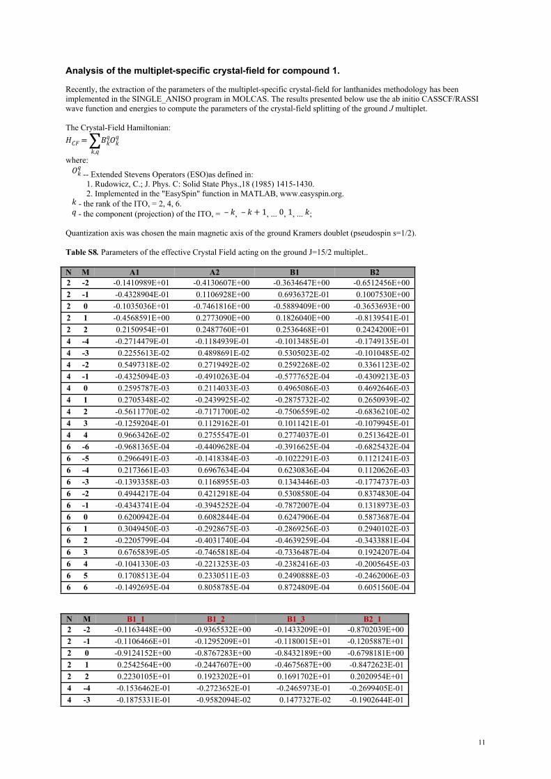
Table S14. Parameters of the effective Crystal Field acting on the ground J=15/2 multiplet..

N M A1 A2 B1 B22 -2 -0.1100617E+01 -0.8495665E+00 -0.7944282E+00 -0.5403544E+002 -1 -0.1263275E+01 -0.1571041E+01 -0.1481225E+01 -0.1550230E+012 0 -0.1855331E+01 -0.1706723E+01 -0.1656034E+01 -0.1567780E+012 1 0.1789891E+01 0.1842430E+01 0.1973693E+01 0.1961580E+012 2 0.2222323E+01 0.1952414E+01 0.1801954E+01 0.1556370E+014 -4 -0.5552456E-02 -0.3170021E-02 -0.4206522E-02 -0.2831343E-024 -3 -0.4142756E-01 -0.4344566E-01 -0.4414281E-01 -0.4338924E-014 -2 -0.2185948E-02 -0.2953800E-02 -0.2961260E-02 -0.3612145E-024 -1 0.1373425E-01 0.7645307E-02 0.6212432E-02 0.2325754E-024 0 -0.2529722E-02 -0.3333255E-02 -0.3243637E-02 -0.3506036E-024 1 -0.1409694E-01 -0.1322193E-01 -0.1419145E-01 -0.1313866E-014 2 0.3276461E-02 0.4583153E-02 0.4321082E-02 0.6302345E-024 3 0.2102724E-01 0.2441880E-01 0.2456039E-01 0.2592791E-014 4 -0.6853751E-02 -0.4621607E-02 -0.3217551E-02 -0.2101587E-026 -6 0.3752403E-03 0.4638362E-03 0.4915720E-03 0.5264023E-036 -5 0.9488541E-04 0.7428196E-04 0.7521113E-04 0.8740109E-046 -4 -0.2436367E-03 -0.1016387E-03 -0.7828901E-04 -0.2787209E-056 -3 -0.7695710E-04 0.1714643E-03 0.2288213E-03 0.2940690E-036 -2 0.7748858E-05 0.1003184E-03 0.1277980E-03 0.1693765E-036 -1 -0.3097644E-04 0.1954744E-03 0.2221243E-03 0.2826276E-036 0 0.2359229E-04 0.1602005E-04 0.1394130E-04 0.2692365E-056 1 0.1716591E-03 0.1312481E-03 0.1217078E-03 0.6989109E-046 2 0.1980115E-03 0.1485446E-03 0.1355973E-03 0.4872083E-046 3 0.2091116E-03 0.2911420E-03 0.2918565E-03 0.2379573E-036 4 0.1454854E-03 0.1089709E-03 0.1078665E-03 0.6847536E-046 5 0.1266315E-02 0.1178342E-02 0.1194514E-02 0.9558949E-036 6 -0.1007068E-03 -0.3522541E-04 -0.4594715E-04 -0.7649587E-05

N M B1_1 B1_2 B2_12 -2 -0.7830653E+00 -0.8786726E+00 -0.4887167E+002 -1 -0.5361899E+00 0.3524916E+00 -0.1355607E+012 0 -0.1418259E+01 -0.1410322E+01 -0.1270537E+012 1 0.1884064E+01 0.1778673E+01 0.1954399E+012 2 0.1384979E+01 0.1030333E+01 0.1245467E+014 -4 -0.8849946E-02 -0.1269648E-01 -0.4876783E-024 -3 -0.4049821E-01 -0.4249427E-01 -0.3985970E-01

17

4 -2 -0.1217658E-02 0.6746897E-03 -0.2876620E-024 -1 0.1725920E-01 0.1505959E-01 0.9194820E-024 0 -0.1563203E-02 0.1722725E-03 -0.3318216E-024 1 -0.1475052E-01 -0.1405937E-01 -0.1339863E-014 2 0.5340884E-02 0.7713271E-02 0.5379467E-024 3 0.1960538E-01 0.1179974E-01 0.2815012E-014 4 -0.7775496E-02 -0.1092831E-01 -0.3605163E-026 -6 0.1946990E-03 0.2996096E-04 0.3882959E-036 -5 0.5703145E-03 0.6620509E-03 0.5239673E-036 -4 -0.2741178E-03 -0.2009884E-03 -0.8891968E-046 -3 -0.3609111E-03 -0.5537759E-03 0.1564096E-036 -2 -0.3947470E-04 -0.9012493E-04 0.1011951E-036 -1 -0.2528309E-03 -0.2018961E-03 0.1721256E-036 0 0.1753904E-04 -0.1397399E-04 0.2226776E-046 1 0.1590443E-03 0.8593203E-04 0.1210636E-036 2 0.9872795E-04 -0.2557835E-03 0.1646759E-036 3 0.5465147E-04 -0.1913764E-03 0.2480077E-036 4 0.2160704E-03 0.1835339E-03 0.1512577E-036 5 0.9311682E-03 0.4388151E-04 0.1152143E-026 6 -0.2425193E-03 -0.2214837E-03 -0.2312127E-03

Recovery factor of the initial energy matrix using the above parameters for each computational model:model Recovery factorA1 98.082969 %A2 98.170025 %B1 98.033505 %B2 97.797277 %B1_1 97.748860 %B1_2 98.050675 %B2_1 97.958687 %

The rest of the energy matrix is accounted by the higher-rank operators (n=8, 10, … , 14).

18

References

1. T. J. Giordano, G. J. Palenik, R. C. Palenik and D. A. Sullivan, Inorg. Chem., 1979, 18, 2445-2450.2. G. M. Sheldrick, SHELXS-97, Program for Crystal Structure Solution, University of Göttingen, (1997), Göttingen, Germany.3. G. M. Sheldrick, SHELXL-97, Program for the refinement of crystal structures from diffraction data, University of Göttingen, (1997), Göttingen, Germany.4. L. J. Farrugia, J. Appl. Cryst., 1999, 32, 837-838.

19