Monoidal Categories - Computer and Information Sciencenoson/MCbeginning.pdf · monoidal categories, ... category theory we learned can describe an entire eld. ... there is a self-contained

Monoidal Categories

A Unifying Concept in

Mathematics, Physics, and Computing

Noson S. Yanofsky

ii

iii

Dedicated to....

iv

It is the harmony of the diverse parts, their symmetry, their happy balance; in a word it is all thatintroduces order, all that gives unity, that permits us to see clearly and to comprehend at once both

the ensemble and the details.Henri PoincaréPage 175 of [79]

Noson S. Yanofskyc©May 2017

Preface

But if you realize all the time what's kind of wonderful - that is, if we expand our experience intowilder and wilder regions of experience - every once in a while, we have these integrations wheneverything's pulled together into a uni�cation, in which it turns out to be simpler than it looked

before.Richard P. Feynman

Page 15 of [30]

Over the past few decades category theory has emerged in many di�erent areas of mathematics,physics, and computer science. The applications of category theory have arisen in (to name just afew �elds) quantum �eld theory, database theory, abstract algebra, formal language theory, quantumalgebra, knot theory, universal algebra, string theory, quantum computing, self-referential paradoxes,M-theory, etc. This book will introduce the category theory necessary to understand large parts ofall these di�erent areas.

Categories are collections of structures and ways of changing those structures. These have beenused to describe many di�erent phenomena in mathematics and science. Our central focus will bemonoidal categories, which are categories with added structure that allow one to describe even morephenomena. The theory of monoidal categories has emerged as a theory of structures and a theoryof processes that change structures. Since category theory is disassociated from any particular �eld,it can deal with many di�erent areas.

Category theory is a simple, extremely clear and concise language in which these various di�erent�elds of science can be discussed. It is also a unifying language. It uni�es di�erent �elds by utilizinga single language where one sees common themes and properties. It also brings together di�erent�elds by actually establishing connections between di�erent �elds of study. Category theory is verygood at showing the �big picture.� Once this language is understood, one is capable of easily learningan immense amount in mathematics, physics, and computing.

This book is an introduction to category theory. It begins with the basic de�nitions of categorytheory and takes the reader all the way up to cutting-edge research topics. Rather than going�down the rabbit hole� with a lot of very technical �pure� category theory, our central focus willbe examples and applications. In fact, an alternate title of this text could be Category Theory ByExample. A major goal is to show the ubiquity of category theory and �nally put an end to thesilly canard that category theory is abstract. Another important goal is to show how many �eldsare related through category theory.

Within each chapter, whenever there is a de�nition or theorem, it is immediately followed by

v

vi

examples and exercises that make the categorical idea clear and come alive. The fun is in theexamples and our examples are from numerous di�erent disciplines.

This text contains fourteen self-contained mini-courses on various �elds. They are short intro-ductions to major �elds such as quantum computing, self-referential paradoxes, quantum algebra,etc. These are sections that do not introduce new categorical ideas. Rather, they show how thecategory theory we learned can describe an entire �eld. The point we are making with these mini-courses is that with the language of category theory in your toolbox, you can master totally newand diverse �elds with ease.

This book is di�erent than other books in category theory. In contrast to them, we do notassume that the reader is already a mathematician, a physicist, or a computer scientist. Rather,this book is for everyone who wants to learn the wonders of category theory. We assume the readeris broad-minded and interested in many areas. We also assume that the reader wants to see howdiverse areas are related to each other. The reader will not only learn a lot of category theory, shewill also learn an immense amount of mathematics, physics, and computers.

Organization

The text commences with an introductory chapter that places category theory in historical andphilosophical context. Chapters 2, 3, and 4 are a simple introduction to category theory. Chapter 2contains the basic de�nitions and properties of categories. Chapter 3 deals with special structureswithin a category. The real magic begins in Chapter 4 where we see how di�erent categories relateto each other.

Chapters 5, 6, and 7 comprise the second part of the book. Chapter 5 describes monoidalcategories which are categories with extra structure. Chapter 6 deals with the relationships betweenmonoidal categories. The core of the book is Chapter 7, where several variations of monoidalcategories are presented with many of their applications.

The �nal three chapters contain some advanced topics. The many categorical ways of describingstructures are dealt with in Chapter 8. Chapter 9 is a collection of more mini-courses from manydi�erent areas. We conclude with Chapter 10, which has a sampling of current research areas inadvanced category theory.

At the end of each chapter, there is a self-contained mini-course on a single topic. The mini-course is given in the language of category theory. Every mini-course ends with several pointers towhere you can learn more about the particular topic.

Appendix A is a giant Venn diagram that shows all of the di�erent types of monoidal categoriesand many of the examples found in the text.

Appendix B is an index of categories that appear in the text.

Appendix C is a guide to further study of category theory and its applications.

Appendix D has answers to selected exercises.

Guide to the Reader

The trick to reading this book is to �nd the examples of the theory that you like the most. Everyreader will probably have a favorite area. We suggest reading the theory part and then focusing onone's area of interest. Our examples are usually seperated into math examples, physics examples,

vii

and computer and logic examples. However, as we shall see, separating these di�erent �elds is noteasy.

Every reader will probably see examples of structures that they already know. They might �ndthose parts slow and pedantic. Please bear with me. Realize that there are others who do not knowthat area well. Learn to skim.

The presentation of some of our categories are spread over the entire book. An example willgrow from being a category, to having certain properties, to having di�erent relationships with othercategories, to being a monoidal category, to having relationships with other monoidal categories, tohaving even more structure, ... If you do not remember seeing a particular category, backtrack towhere it was �rst mentioned. Read the book with a �nger in Appendix B to �nd earlier referencesto that category. Also, it is wise to keep an eye on the Venn diagram in Appendix A. There youwill see what structures a category has and its relation with other structures.

If there is a particular example or idea in a certain �eld that interests you, consider looking atAppendix C to see where you can �nd more information about those concepts.

The reader is strongly urged to do all the exercises in the book. The only way to have categorytheory at your �ngertips is to do category theory!

Ancillaries

This text does not stand alone. I maintain a web page for the text atwww.sci.brooklyn.cuny.edu/noson/mctext. The web page will contain:

(a) periodic updates of the book;(b) links to interesting books and articles on category theory and monoidal categories;(c) some answers to certain exercises not solved in Appendix D; and(d) errata.

The reader is encouraged to send any and all corrections and suggestions [email protected] me make this book better!

Acknowledgment

Eugene Dorokhin, Michael Goldenberg, Jonathan Hanon, Deric Kwok, Moshe Lach, ArmandoMatos, and Brian Porter were all very helpful in the editing process of this text.

viii

Contents

Preface v

Organization . . . . . . . . . . . . . . . . . . . . . . . . . . . . . . . . . . . . . . . . . . . vi

Guide to the Reader . . . . . . . . . . . . . . . . . . . . . . . . . . . . . . . . . . . . . . . vi

Ancillaries . . . . . . . . . . . . . . . . . . . . . . . . . . . . . . . . . . . . . . . . . . . . . vii

Acknowledgment . . . . . . . . . . . . . . . . . . . . . . . . . . . . . . . . . . . . . . . . . vii

1 Introduction 1

1.1 Categories . . . . . . . . . . . . . . . . . . . . . . . . . . . . . . . . . . . . . . . . . . 1

1.2 Monoidal Categories . . . . . . . . . . . . . . . . . . . . . . . . . . . . . . . . . . . . 4

1.3 The Examples and the Mini-Courses . . . . . . . . . . . . . . . . . . . . . . . . . . . 5

1.4 Notation . . . . . . . . . . . . . . . . . . . . . . . . . . . . . . . . . . . . . . . . . . . 6

1.5 Mini-course: Categorical Thinking . . . . . . . . . . . . . . . . . . . . . . . . . . . . 7

2 Categories 29

2.1 Basic De�nitions and Examples . . . . . . . . . . . . . . . . . . . . . . . . . . . . . . 29

2.2 Basic Properties . . . . . . . . . . . . . . . . . . . . . . . . . . . . . . . . . . . . . . 49

2.3 Related Categories . . . . . . . . . . . . . . . . . . . . . . . . . . . . . . . . . . . . . 55

2.4 Mini-Course: Linear Algebra . . . . . . . . . . . . . . . . . . . . . . . . . . . . . . . 58

3 Structures Within Categories 79

3.1 Products and Coproducts . . . . . . . . . . . . . . . . . . . . . . . . . . . . . . . . . 79

3.2 Limits and Colimits . . . . . . . . . . . . . . . . . . . . . . . . . . . . . . . . . . . . 91

3.3 Slices and Coslices . . . . . . . . . . . . . . . . . . . . . . . . . . . . . . . . . . . . . 98

3.4 Mini-Course: Self-Referential Paradoxes . . . . . . . . . . . . . . . . . . . . . . . . . 100

4 Relationships Between Categories 123

4.1 Functors . . . . . . . . . . . . . . . . . . . . . . . . . . . . . . . . . . . . . . . . . . . 123

4.2 Natural Transformations . . . . . . . . . . . . . . . . . . . . . . . . . . . . . . . . . . 135

4.3 Equivalences . . . . . . . . . . . . . . . . . . . . . . . . . . . . . . . . . . . . . . . . 138

4.4 Adjunctions . . . . . . . . . . . . . . . . . . . . . . . . . . . . . . . . . . . . . . . . . 139

4.5 Exponentiation . . . . . . . . . . . . . . . . . . . . . . . . . . . . . . . . . . . . . . . 143

4.6 Limits and Colimits Revisited . . . . . . . . . . . . . . . . . . . . . . . . . . . . . . . 146

4.7 Comma Categories . . . . . . . . . . . . . . . . . . . . . . . . . . . . . . . . . . . . . 147

4.8 The Yonada Lemma . . . . . . . . . . . . . . . . . . . . . . . . . . . . . . . . . . . . 148

4.9 Mini-Course: Basic Categorical Logic . . . . . . . . . . . . . . . . . . . . . . . . . . 150

ix

x CONTENTS

5 Monoidal Categories 151

5.1 De�nitions and Basic Properties . . . . . . . . . . . . . . . . . . . . . . . . . . . . . . 151

5.2 Cartesian Categories . . . . . . . . . . . . . . . . . . . . . . . . . . . . . . . . . . . . 152

5.3 Strict Monoidal Categories . . . . . . . . . . . . . . . . . . . . . . . . . . . . . . . . . 152

5.4 Mini-Course: Quantum Computing . . . . . . . . . . . . . . . . . . . . . . . . . . . . 153

6 Relationships Between Monoidal Categories 155

6.1 Monoidal Functors and Monoidal Natural Transformations . . . . . . . . . . . . . . . 155

6.2 MacLane's Coherence Theorems . . . . . . . . . . . . . . . . . . . . . . . . . . . . . . 160

6.3 Joyal and Street's Coherence Theorems . . . . . . . . . . . . . . . . . . . . . . . . . . 160

6.4 When Coherence Fails . . . . . . . . . . . . . . . . . . . . . . . . . . . . . . . . . . . 160

6.5 Mini-Course: Information Theory . . . . . . . . . . . . . . . . . . . . . . . . . . . . . 161

7 Variations of Monoidal Categories 163

7.1 Braided Monoidal Categories . . . . . . . . . . . . . . . . . . . . . . . . . . . . . . . 163

7.2 Symmetric Monoidal Categories . . . . . . . . . . . . . . . . . . . . . . . . . . . . . . 164

7.3 Cartesian Categories . . . . . . . . . . . . . . . . . . . . . . . . . . . . . . . . . . . . 164

7.4 Closed Categories . . . . . . . . . . . . . . . . . . . . . . . . . . . . . . . . . . . . . . 164

7.5 Compact Categories . . . . . . . . . . . . . . . . . . . . . . . . . . . . . . . . . . . . 164

7.6 *-Autonomous Categories . . . . . . . . . . . . . . . . . . . . . . . . . . . . . . . . . 165

7.7 Categories with Traces . . . . . . . . . . . . . . . . . . . . . . . . . . . . . . . . . . . 165

7.8 Mini-Course: Quantum Algebra . . . . . . . . . . . . . . . . . . . . . . . . . . . . . . 165

8 Describing Structures 167

8.1 Algebraic Theories . . . . . . . . . . . . . . . . . . . . . . . . . . . . . . . . . . . . . 167

8.2 Monads . . . . . . . . . . . . . . . . . . . . . . . . . . . . . . . . . . . . . . . . . . . 167

8.3 Operads . . . . . . . . . . . . . . . . . . . . . . . . . . . . . . . . . . . . . . . . . . . 167

8.4 2-Algebraic Theories . . . . . . . . . . . . . . . . . . . . . . . . . . . . . . . . . . . . 168

8.5 Mini-Course: Knot Invariants . . . . . . . . . . . . . . . . . . . . . . . . . . . . . . . 168

9 More Mini-Courses 169

9.1 Mini-Course: Theoretical Computer Science . . . . . . . . . . . . . . . . . . . . . . . 170

9.2 Anyon Computation . . . . . . . . . . . . . . . . . . . . . . . . . . . . . . . . . . . . 209

9.3 Linear Logic . . . . . . . . . . . . . . . . . . . . . . . . . . . . . . . . . . . . . . . . 209

9.4 Loop Quantum Gravity . . . . . . . . . . . . . . . . . . . . . . . . . . . . . . . . . . 209

9.5 TQFT . . . . . . . . . . . . . . . . . . . . . . . . . . . . . . . . . . . . . . . . . . . . 209

9.6 Abramsky and Coecke . . . . . . . . . . . . . . . . . . . . . . . . . . . . . . . . . . . 209

9.7 The Standard Model . . . . . . . . . . . . . . . . . . . . . . . . . . . . . . . . . . . . 209

10 Advanced Topics 211

10.1 Kan Extensions . . . . . . . . . . . . . . . . . . . . . . . . . . . . . . . . . . . . . . . 211

10.2 Enriched Category Theory . . . . . . . . . . . . . . . . . . . . . . . . . . . . . . . . . 211

10.3 Advanced Structures in Categories . . . . . . . . . . . . . . . . . . . . . . . . . . . . 211

10.4 Higher Category Theory . . . . . . . . . . . . . . . . . . . . . . . . . . . . . . . . . . 211

10.5 Topos Theory . . . . . . . . . . . . . . . . . . . . . . . . . . . . . . . . . . . . . . . . 212

10.6 Homotopy Theory . . . . . . . . . . . . . . . . . . . . . . . . . . . . . . . . . . . . . 212

CONTENTS xi

10.7 Homotopy Type Theory . . . . . . . . . . . . . . . . . . . . . . . . . . . . . . . . . . 212

Appendix A: Venn Diagram of Types of Monoidal Categories 213

Appendix B: Index of Categories 215

Appendix C: Guide to Further Study 217

Appendix D: Answers to Selected Problems 221

Bibliography 231

Index 232

xii CONTENTS

Chapter 1

Introduction

The language of categories is a�ectionately known as abstract nonsense, so named by NormanSteenrod. This term is essentially accurate and not necessarily derogatory: categories refer to

nonsense in the sense that they are all about the `structure', and not about the `meaning', of whatthey represent.

Paolo Alu�Page 18 of [1]

1.1 Categories

Category theory began with the intention of relating two di�erent areas of study. The aim was tocharacterize and classify certain types of geometric objects by assigning to each of them certaintypes of algebraic objects (see Figure 1.1). (In detail, the geometric objects were structures calledtopological spaces, manifolds, bundles, etc. The algebraic objects were called groups, rings, abeliangroups, etc. The assignments had exotic names like homology, cohomology, homotopy and K-theory, etc.) Researchers realized that if they were going to relate geometric objects with algebraicobjects they needed a language that is neither specialized to a geometric content nor an algebraiccontent. Only with such a general language can one speak of both �elds. The language inventedby Samuel Eilenberg and Saunders Mac Lane [27] used various collections. Each collection wascalled a category. There was a collection of geometric objects and a collection of algebraic objects.They were interested in many di�erent categories and in order to relate one category with another,they formulated the notion of a functor which � like a function � assigns to each entity in onecategory an entity in another category. They went further and formulated the notion of a naturaltransformation which is a way of relating di�erent functors between categories. (In a sense, anatural transformation transfers the results of one functor into the results of another functor.) Onemight visualize these structures as in Figure 1.2 which shows category A and category B. Relatingthese categories are functor F and functor G. And, �nally, relating these functors is a naturaltransformation α.

What is a category? It is not simply a collection of structures (called objects) of a particulartype. Rather, a category is a collection of objects and transformations or processes between theobjects. We call these transformations or processes morphisms or maps. We can visualize partof an example of a category as Figure 1.3. The letters correspond to the objects and the arrows

1

2 CHAPTER 1. INTRODUCTION

Geometric Objects Algebraic Objects

• •homology // • • •

• •cohomology// •

•homotopy // •

• • •... // • •

(1.1)

Figure 1.1: Relating geometric objects to algebraic objects.

correspond to the morphisms between objects. These morphisms are to be thought of as ways oftransforming objects. As time went on, the morphisms between objects took central stage. Categorytheory not only became the study of structures but also the study of transformations or processeson structures. One of the main properties of processes is that they can be combined. One processfollowed by another process can be combined into a single process. In a category, if there is amorphism from object a to object b called f and a morphism from object b to object c called g,then there will be an associated morphism from object a to object c written as g ◦ f and called �gcomposed f � or �g following f � or �g after f .� This can be drawn as follows:

af //

g◦f

&&b

g // c. (1.2)

This is one of the de�ning properties of a category. We shall see the others in a few pages.

category A

functor F

++

functor G

33natural transformation α ⇓ category B. (1.3)

Figure 1.2: Categories, functors and natural transformations.

Categories are related to more familiar structures called (directed) graphs and groups. A graphis a structure that has objects (vertices) and morphisms (arrows) between them. One can view a

1.1. CATEGORIES 3

...

c

id

��d

id

��

a

77id

��

· · · a′

''

id

��

99 PP

· · ·

b

id

��

55

e

id

��

wwb′

id

��

..EE

a′′

xxkk

id

��

c′

WW

id

��

..EE

...

(1.4)

Figure 1.3: An example of part of a category.

category as a souped-up graph. Categories, like graphs, also have objects and morphisms, but withincategories, certain morphisms can be composed. A graph is used to deal with various phenomenaof interconnectivity. A category, with its extra structure, will deal with a more sophisticated notionof interconnectivity. A category can also be seen as a generalization of a group (more properlyof a monoid, however monoids are less well known than groups). Group theory is the science ofcombining entities. A group is a set where one can combine two elements to form other elements. Ina category, one can combine morphisms that follow one another. This combining can be thought ofas having one process follow another process. Graphs and groups are ubiquitous in modern scienceand mathematics. Categories � as generalizations of both structures � are even more pervasive.

Since categories are disassociated from any speci�c �eld or area, category theory received thereputation of being a language without content or �general abstract nonsense.� However, it wasprecisely this independence from any �eld which gave category theory its power. By not beingformulated for one particular �eld, it is capable of dealing with any �eld. At �rst category theorywas extremely successful in dealing with various �elds of mathematics. As time went on, it was


realized that many branches of science that deal with structures or processes can be discussed inthe language of category theory. Computer science is the study of computational processes, andhence, has taken a deep interest in category theory. More recently, category theory has been shownto be very adept at discussing structures and processes in physics. In the coming pages, we shallalso see examples of structures and processes from chemistry, biology, and linguistics.

Many diverse �elds are shown to be related because they are discussed in the single language ofcategory theory. Researchers have found similar theorems and patterns in areas that were thought tobe unrelated. Moreover, in the past few decades, category theory has been further unifying di�erent�elds by showing that there are actual amazing relationships between these various �elds. Thereare functors from a category in one �eld to a category in a totally di�erent �eld. These functorspreserve properties and structures that show a uni�cation of �elds. For example, quantum algebrais a �eld that uses categorical language to show how certain algebraic structures are related togeometric structures like knot theory. Another prominent example is quantum �eld theory, which isa branch of physics that uses functors to unite relativity and quantum theory. Quantum computingis a �eld that sits at the intersection of computer science, physics, and mathematics and which canbe understood with various categorical structures.

1.2 Monoidal Categories

Monoidal categories are categories with extra structure. In the early 1960s, Jean Bénabou andSaunders Mac Lane realized that there are categories that have more structure. In certain categories,one can �multiply� or �combine� objects. Such categories were called monoidal categories. Insymbols, within a monoidal category, object a and object b can be combined to form object a ⊗ b(read �a tensor b�). As always in category theory, one is not only interested in combining objectsbut also in combining morphisms. If there are morphism f : a −! a′ and morphism g : b −! b′,then there will be objects a⊗ b and a′ ⊗ b′. In addition there will also be a morphism

f ⊗ g : (a⊗ b) −! (a′ ⊗ b′). (1.5)

Notice that there are two ways of combining morphisms in a monoidal category. There is f ◦ gand there is f ⊗g. In physics, the combination f ◦g will correspond to performing one process afteranother while the combination f ⊗ g will correspond to performing two independent processes. Incomputers, the combination f ◦g will correspond to sequential processes, while f⊗g will correspondto parallel processes. In math, the interplay of the two combinations of morphisms will be veryimportant.

Classical algebra is the branch of mathematics that deals with sets and operations on those sets.For sets of numbers and the addition operation, we have the rule that x+y = y+x while in generalx−y 6= y−x. In the theory of monoidal categories we must ask for rules that govern the relationshipbetween a ⊗ b and b ⊗ a. What about the relationship between (a ⊗ b) ⊗ c and a ⊗ (b ⊗ c)? Inmonoidal categories there are many more possible answers than when dealing with sets of numbersand their operations. For every possible answer, there will be a di�erent type of monoidal category.In Chapter 7, we will see many di�erent types of monoidal categories. This variability ensures thatmany phenomena can be described by monoidal categories. The area that deals with the di�erenttypes of rules is called �coherence theory� (i.e., how the various operations cohere with each other)or �higher-dimensional algebra.� This type of algebra has become ubiquitous and it is believed that

1.3. THE EXAMPLES AND THE MINI-COURSES 5

higher-dimensional algebra will arise even more frequently in the science and mathematics of thecoming decades.

1.3 The Examples and the Mini-Courses

This book is centered on the examples. Our goal is to show the pervasiveness of categories, andin particular monoidal categories. We also want to emphasize how categories demonstrate theinterconnectedness of various �elds. We do this by introducing lots of examples from many di�erentareas. Immediately following a de�nition or a theorem of category theory there are lots of examplesthat illustrate the idea. There are also some examples that are left to the reader as exercises. It isimportant to realize that although this book is chock-full of examples, we have barely scratched thesurface. The literature of category theory has many more examples. We chose the examples thatarise most frequently or are the easiest to understand. The reader will be directed to places in theliterature where other examples are described. We are showing the beauty of category theory butonly revealing the tip of the iceberg.

Most of the examples can be loosely split into three broad groupings: mathematics, physics,and computers. There will also be examples from �elds like chemistry, biology, and linguistics. Theproblem is that the boundaries between these di�erent areas are hazy. For example, is quantumcomputing part of computer science, physics or abstract mathematics? Is knot theory part ofmathematics or physics? There are no simple answers to these questions.

Since most readers are familiar with sets and functions between sets, we usually try to �rstshow an idea or de�nition in terms of sets. In later chapters, it will become apparent that setsand functions between sets are not the right context to examine certain phenomena. This is wherecategory theory really gets interesting.

The examples are spread throughout the book. To illustrate, in Chapter 2, a category of logicalcircuits will be introduced. In Chapter 3, some properties of this category will be described. Thiscategory will be related to other categories in Chapter 4. In Chapter 5 we will show that the categoryof logical circuits has a monoidal structure, and we will see how that monoidal structure relates withthe monoidal structure of other categories in Chapter 6. This same category and variations of thiscategory will be shown to have even more structure in Chapter 7. We will also see how this simplecategory arises in the mini-course on quantum computing and theoretical computer science. By thetime the reader �nishes the book, the category of logical circuits will be an old friend. The categoryof logical circuits is just one such example. However, in order not to have too much material in thebeginning, we will introduce many categories in later chapters as well. Our aim is readability.

These examples will take the reader rather far. In mathematics, the reader will meet lots ofalgebra and topology. In physics we will see the basics of quantum theory as well as some stringtheory and quantum �eld theory. In computers we will see how categories are good for describingcertain models of computation and some advanced logic.

Due to space limitations and by concentrating on examples, we are going to omit some resultsin pure category theory. We only do the category theory required to understand the examples. InAppendix C we point out various places where one can learn more (pure) category theory.

Category theory is a language that can deal with many di�erent areas of science. The really funpart of category theory is that once one has this language in their toolbox, they can easily pick upwhole new branches of science. We show this with little mini-courses. At the end of every chapteris a little self-contained section that describes whole �elds with the category theory already learned.


Mini-courses in later chapters depend on the knowledge of earlier mini-courses. In Chapter 9, weo�er several other mini-courses. At the end of each mini-course, we will point out where to learnmore about that particular topic.

It must be noted that this is not a history book. We are not going to say who thought ofsome particular construction or example �rst. Some of the examples in this book came from otherbooks and papers. Some examples are just known in the folklore of category theory. And someexamples, we made up. The history is too complicated for us to disentangle and is of absolutelyno pedagogical use to the novice. We will name some places to learn about the history of categorytheory in Appendix C.

This book owes a tremendous debt to previous works.

• I �cut my teeth� learning category theory from Saunders Mac Lane's Categories for the WorkingMathematician [65]. This is the classic text by one of the founders of category theory. It is avision of clarity! It in�uenced my thinking and this book in the most profound way. As thetitle implies, Mac Lane assumes that the reader knows a lot of mathematics before openinghis book. My goal in this book is to give over the beauty of category theory as Mac Lane didbut for a wider audience.• John Baez and Michael Stay wrote an wonderful paper �Physics, Topology, Logic and Com-putation: A Rosetta Stone� [7] that highlights the connections between many di�erent �elds.I would like to think of this book as an explanation and an expansion of that paper.• I learned a lot from Christian Kassel's text book Quantum Groups [46]. His clarity andexactness is an inspiration.• This book attempts to be as readable as Michael Barr and Charles Wells' textbook CategoryTheory for Computing Science [9]. That work goes through a lot of category theory with manyexamples along the way. We try to do the same.

There are many potential topics that could have gone into this book. Painful choices had to bemade. In the end, topics were chosen based on personal preference. I would like to believe that thetopics chosen will be important as we march into the unfathomable future.

Finally, I would like to apologize to all my friends in the category theory community if I neglectedtheir favorite example or did not discuss an area in which they did great work. It was not myintention to omit anyone's work. I hope they can �nd it in their hearts to forgive this poor sinner.

1.4 Notation

In order to improve readability, for the most part, we keep to the following notation.

• Categories are in boldface: A,B,C,D,Circuit,Set, . . .• Objects in general categories are the �rst few lowercase Latin letters: a, b, c, d, a′, b′, a′′ . . .• Morphisms in general categories are lowercase Latin letters: f, g, h, i, j, k, f ′, g′′, . . .• Functors are capital Latin letters: F,G,H, I, J, . . .• Natural transformations are lowercase Greek letters: α, β, γ, δ, η, κ, . . .• Higher dimensional morphisms will be capital Greek letters: Γ,∆,Θ,Φ,Ψ, . . .• Sets of numbers are N ,Z,Q,R, C.

1.5. MINI-COURSE: CATEGORICAL THINKING 7

1.5 Mini-course: Categorical Thinking

Category theory is not just a language that is capable of describing an immense amount of scienceand mathematics. Rather, it is a way of thinking. One of the central ideas in category theory isthat the morphisms of a category help describe the properties and the structure of the objects in acategory.

Important Categorical Idea 1.5.1 Properties and structures in a category can be de-scribed by the morphisms of the category. That is, the objects do not stand alone. Onemust see how the objects relate to each other with morphisms. The objects have to beseen in context of the morphisms. ©

In order to get a feel for this, we take an in-depth look at the familiar world of sets and functionsbetween sets. We show that a lot of the usual ideas and constructions about sets can be describedwith functions between sets. This mini-course will also be a gentle reminder of a lot of conceptsthat are needed in the rest of the text.

I am grateful to Ralph Wojtowicz for recommending that I write this mini-course and stressingits importance for a new student of category theory.

Sets

A set is a collection of elements. If S is a set and x is an element of S, we write x ∈ S. If x is notan element of S we write x 6∈ S. We will deal with both in�nite sets and �nite sets. Some of themost important in�nite sets of numbers are

• The natural numbers, N = {0, 1, 2, 3, . . .}.• The integers, Z = {. . . ,−3,−2,−1, 0, 1, 2, 3, . . .}.• The rational numbers, Q = {mn : m and n in Z and n 6= 0}.• The real numbers, R, that is, all numbers on the real number line.• The complex numbers, C = {a+ bi : a and b in R}.

The most interesting property about a �nite set is the number of elements in the set. For everyset S, we write |S| to denote the number of elements in S.

Let S and T be sets. If s is in S and t is in T we write an ordered pair of the elements as(s, t). The set of all ordered pairs is called the Cartesian product of S and T

S × T = {(s, t) : s ∈ S, t ∈ T}. (1.6)

Example 1.5.1. If Pants = {black, blue1, blue2, gray} is the set of pants that you own, andShirts = {t-shirt1, t-shirt2, polo-shirt} is the set of shirts that you own, then the set of Out�ts is

Pants× Shirts =

(black, t-shirt1), (black, t-shirt2), (black, polo-shirt),

(blue1, t-shirt1), (blue1, t-shirt2), (blue1, polo-shirt),

(blue2, t-shirt1), (blue2, t-shirt2), (blue2, polo-shirt),

(gray, t-shirt1), (gray, t-shirt2), (gray, polo-shirt)

(1.7)


(True scholarly category theorists do not care if their clothes fail to match!) �

Technical Point 1.5.1 One must realize that the most important idea of an ordered pair is itsorder. In contrast, sets are just collections and as such do not have an order. The set {s, t} isconsidered to be the same set as {t, s}. So we cannot simply use curly brackets to describe orderedpairs. We need something new like (s, t). The pair (s, t) is not considered the same as (t, s). Thereare other ways of describing an ordered pair of elements from S and T . For example, we could writethem as 〈s, t〉 or {s, t, {s}} (where we collect the elements but indicate the �rst element by puttingit into a set by itself), or even {s, t, {t}} (where we indicate the second element by putting it into aset by itself). There is nothing special about the notation (s, t). (We will see why this is importantin Section 3.1) ♥

If there are m elements in S and n elements in T then there are mn elements in S × T . Insymbols we write this as

|S × T | = |S||T |. (1.8)

Exercise 1.5.1. How many elements were in Pants? How many elements were in Shirts? Howmany elements in Out�ts? Show that the above formula works.

Solution: 4,3,12 = 4× 3.

�

We can generalize the notion of ordered pairs to ordered triples, ordered 4-tuples, or-dered 5-tuples, etc. If there are n sets, S1, S2, . . . , Sn, then an ordered n-tuple is written as(s1, s2, . . . sn) where si is in Si. The set of all n-tuples is S1×S2×· · ·×Sn. The number of n-tuplesfollows a generalization of Equation 1.8:

|S1 × S2 × · · · × Sn| = |S1||S2| · · · |Sn|. (1.9)

Exercise 1.5.2. In addition to pants and shirts, an out�t might consist of a hat, socks, and shoes.In this case, show how many out�ts there are given that there are m hats, n pairs of socks, p pairsof shoes, q pants and r shirts.

Solution: m× n× p× q × r.�

Let S and T be sets. The union of S and T is the set S⋃T which contains those elements that

are in S or in T .

S⋃T = {x : x ∈ S or x ∈ T}. (1.10)

It is important to notice that if there is some element that is in both S and in T then it will occuronly once in S

⋃T . This is because when dealing with a set, repetition does not matter. The set

{a, b, c, b} is considered the same set as {a, b, c}.Another operation is the disjoint union which contains the elements from S and the elements

from T but considers elements that are in both as di�erent elements. The way this is done is bytagging every element with the extra information that says which set it comes from. This way anelement that is both in S and in T would be considered two di�erent elements. For example, ifS = {a, b, c, x, y} and T = {q, w, b, x, e, r}, then

S∐

T = {(a, 0), (b, 0), (c, 0), (x, 0), (y, 0), (q, 1), (w, 1), (b, 1), (x, 1), (e, 1), (r, 1)} (1.11)


where the elements of S are tagged with a 0 and the elements of T are tagged with a 1. In generalfor sets S and T , we have

S∐

T = (S × {0})⋃

(T × {1}) (1.12)

The formula for the number of elements in the disjoint union is |S∐T | = |S|+ |T |.

Exercise 1.5.3. When does the union of two sets have the same number of elements as the disjointunion of those same sets?

Solution: When the intersection is empty.�

Functions

The central idea of this mini-course is the notion of functions between sets.

De�nition 1.5.1. Let S and T be sets. A function, f , from S to T , written f : S −! T is a rulethat assigns to every element of S an element of T . The value of f on the element s is written asf(s). If f(s) = t we write s 7! t. ♦

It is important to understand the di�erence between the symbol −! and the symbol 7!. The−! symbol goes between two sets. It describes a function from one set to another. In contrast, thesymbol 7! goes from an element in the �rst set to an element in the second set. It describes howthe function is de�ned.

Example 1.5.2. For every set S, there is an identity function idS : S −! S which takes everyelement to itself. In symbols it is de�ned as idS(s) = s. �

Functions can be used as a way of describing or choosing elements of a set. Consider a oneelement set {∗}. (There are many one element sets such as {a}, {b} , {Bill}, etc.) For a set S, afunction f : {∗} −! S picks out one element of S. The single element ∗ goes to s in S. In symbols,f(∗) = s or ∗ 7! s.

Example 1.5.3. Let S be the set {Jack, Jill, Joane, June, Joe, John}. The element Joe in S can bedescribed as a function f : {∗} −! S where f(∗) = Joe. We might want to distinguish this functionby calling it fJoe : {∗} −! S. There will be other functions like fJill : {∗} −! S where fJill(∗) =Jill. For this set of six elements, there will be six di�erent functions from {∗} to S. �

If one was interested in choosing two elements of S we can look at functions from a two elementset to S. So f : {0, 1} −! S will choose two elements of S. If f(0) 6= f(1) then f will choosetwo di�erent elements of S. The �rst element is f(0) and the second element is f(1). Every suchfunction chooses two elements of S. Functions from {a, b, c} to S will choose three elements of S.This can go on: if we wanted to choose n elements of a set, we would look at functions of the form

{1, 2, . . . , n} −! S. (1.13)

De�nition 1.5.2. T is a subset of S if every element of T is an element of S. We write this asT ⊆ S. If T is a subset of S but not equal to S, we call T a proper subset and write T ( S. If Tis a subset of S, there is an inclusion function that takes every element of T to its corresponding


element of S and is written as inc : T ↪−! S. There is a special set that has no elements. It is calledthe empty set and is denoted ∅. The empty set is a subset of every set. ♦

De�nition 1.5.3. For a set S, the set of all subsets of S is called the powerset of S and is denotedP(S). ♦

Example 1.5.4. For the set {a}, the powerset is P({a}) = {∅, {a}}. The powerset of a twoelement set is P({a, b}) = {∅, {a}, {b}, {a, b}}. The powerset of a three element set is P({a, b, c}) ={∅, {a}, {b}, {c}, {a, b}, {a, c}, {b, c}, {a, b, c}}. Whenever we add an element to a set, we double thenumber of elements in the powerset. There is the following rule: if S has n elements, then P(S) has2n elements. In symbols, |S| = n implies |P(S)| = 2n. We can also write this as |P(S)| = 2|S|. �

Functions can also be used to describe subsets. For any set S and subset T there is an associatedcharacteristic function χT : S −! {0, 1} which assigns each element s of set S to 1, if s is in T ,and 0 if s is not in T , i.e.,

χT (s) =

1 : s ∈ T

0 : s 6∈ T.(1.14)

(χ is a Greek letter �chi� that sounds like the �rst syllable of �characteristic�.) χT is a function thattells which elements of S are in T and which elements are not in T .

Example 1.5.5. Let S be the set {Jack, Jill, Joane, June, Joe, John}. Consider the subsetT = {Jack, Joe, John} of S that contains all the boys in S. This subset can be described by thefunction χT : S −! {0, 1} which can be visualized as

Jack �

++

Jill}

��

1

Joane �

++

June �

))0

Joe5

::

JohnA

@@

(1.15)

�

Exercise 1.5.4. For the sets of numbers, we know that N ( Z ( Q ( R ( C. Give thecharacteristic function for each of these proper subsets.

Solution: Let us just focus on the subset Q ( R. The characteristic function χQ : R −! {0, 1}


is de�ned as follows:

χQ(r) =

1 : r is rational

0 : r is not rational.(1.16)

The others are done similarly.

�

A characteristic function assigns the elements of S one of two possible values. There might be aneed to assign one of many values to every element of S. For example, a function S −! {a, b, c, d}assigns to every element of S one of these letters which can stand for di�erent things. In general, afunction

S −! {1, 2, . . . , n} (1.17)

assigns every element of S one of n numbers. We can also assign to every element of S an elementof [0, 1], the real interval between 0 and 1. This can correspond to assigning a probability to everyelement.

Example 1.5.6. In school, every student usually has an associated grade point average (GPA).This is written as a function Students −! [0, 4]. �

If S is a set, then there is a function called the diagonal function ∆: S −! S×S which takesevery element to an ordered pair of the same element. In symbols, for s in S we have

∆(s) = (s, s). (1.18)

If f : S −! S′ and g : T −! T ′ are functions then there exists a function f×g : S×T −! S′×T ′that takes an ordered pair of elements and applies f to the �rst element and g to the second. Insymbols, the function is de�ned for elements s of S and t of T as

(f × g)((s, t)) = (f(s), g(t)) ∈ S′ × T ′. (1.19)

In a sense, this process is a parallel process. We process s with f and t with g.

Exercise 1.5.5. Let f : N −! R be de�ned by f(n) =√n and g : R −! Z be de�ned by

g(r) = prq. What is (f × g)((5,−5.1))

Solution: (√

(5),−5).

�

De�nition 1.5.4. There are some special types of functions. We say f : S −! T is

• one-to-one or injective if di�erent elements in S go to di�erent elements in T . That is, forall s and s′ in S, if s 6= s′ then f(s) 6= f(s′). Another way to say this is that if f(s) = f(s′)then it must be that s = s′. In English, this means that if the function takes elements to thesame output, the elements must have started o� equal.• onto or surjective if for every element t in T , there is an s in S such that f(s) = t.• an isomorphism or a one-to-one correspondence or a bijection if f is one-to-one andonto. That is, for every element s of S there is a unique element t of T so that f(s) = t andfor every element t of T there is a unique element s of S so that f(s) = t.


♦

De�nition 1.5.5. Sets S and T are isomorphic if there is an isomorphism between them. Wewrite this as S ' T . ♦

Exercise 1.5.6. Explain why two �nite sets that have the same number of elements are isomorphic.

Solution: It is easy to make an isomorphism from one set to the other.�

Exercise 1.5.7. Show that R×R is isomorphic to C.Solution: The isomorphism will take (r1, r2) ∈ R×R to r1 + ir2 ∈ C.

�

One of the central ideas in set theory is that given sets S and T we can form a set which consistsof all functions from S to T . We denote this set of functions as Hom(S, T ) or TS .

Exercise 1.5.8. Write down the set of all the functions from the set {a, b, c} to the set {0, 1}.Solution: Each of the following lines is a function.

f(a) = 0 f(b) = 0 f(c) = 0

f(a) = 0 f(b) = 0 f(c) = 1

f(a) = 0 f(b) = 1 f(c) = 0

f(a) = 0 f(b) = 1 f(c) = 1

f(a) = 1 f(b) = 0 f(c) = 0

f(a) = 1 f(b) = 0 f(c) = 1

f(a) = 1 f(b) = 1 f(c) = 0

f(a) = 1 f(b) = 1 f(c) = 1

�

We saw that every element in a set S can be described as a function {∗} −! S. The correspon-dence between elements of S and functions from {∗} to S shows that

S ' S{∗} = Hom({∗}, S) (1.20)

Using characteristic functions, we saw that there is a correspondence between subsets of S andfunctions from S to 2 = {0, 1}. This correspondence can be stated as

P(S) ' 2S = Hom(S, 2) (1.21)

Example 1.5.7. Consider the simple binary addition operation +: N × N −! N . Let us writethis function with its inputs clearly marked as follows

( ) + ( ) : N ×N −! N . (1.22)


Now consider the function ( )+5: N −! N . This is a function with only one input. We could alsomake another function of one variable ( ) + 7: N −! N . In fact we can do this for any naturalnumber. We can de�ne a function that inputs a natural number and outputs a function from naturalnumbers to natural numbers. That is, there is a function Φ: N −! Hom(N ,N ) which is de�nedas Φ(n) = ( ) + n. It is easy to see that the + operation is built up from all the Φ(n).

Notice that what we said about + really applies to every function with two inputs. If f : T ×U −! S is a function from T × U then for every u ∈ U there is a function f( , u) : T −! S. Thisshows that there is a function Φ: U −! Hom(T, S). It is easy to see that any function f is builtup from all the Φ(u) functions. �

This example brings to light the following important theorem about sets.

Theorem 1.5.1. For sets S, T and U there is the following isomorphism ST×U ' (ST )U or

Hom(T × U, S) ' Hom(U,Hom(T, S)) (1.23)

F

Proof. To show that these two sets are isomorphic, consider f : T × U −! S. From this functionlet us de�ne an f ′ : U −! Hom(T, S). For a u in U we have the function f ′(u) : T −! S which isde�ned as follows: for t in T , set f ′(u)(t) = f(t, u). This function has the same information as f .It is not hard to go from f ′ back to f . ♣

Let us count how many functions there are between two �nite sets. Consider S with |S| = mand T with |T | = n Consider a function f : S −! T . For each element s in S there are n possiblevalues of f(s) in T . For two elements in S there are n × n possibilities of choices in T . In total,there are n× n× · · · × n (m times) possible maps. So

|Hom(S, T )| = |TS | = nm = |T ||S|. (1.24)

Operations on Functions

There are many times that we are going to take two functions and perform an operation to get athird function. Three such operations are composition, extension and lifting. Remarkably, manyideas about functions can be understood as operations in one of these three forms.

The simplest operation is composition. If there is a function f : S −! T and a functiong : T −! U , then the composition of them is a function h = g ◦ f : S −! U that is de�ned on a sin S as h(s) = g(f(s)). We write these functions as

Sf //

h=g◦f

��

T

g

��U.

(1.25)


This diagram is a called a commutative diagram. It means that if you start with any elements in S and you apply the two functions from S to U , you will get to the same resulting elementin U . In detail, for all s, we have that g(f(s)) = h(s). There will be many such diagrams in thecoming pages. In all the cases, start from any set and follow all the paths of composible functionsand you will get the same element. Throughout this text, unless otherwise stated, all diagrams arecommutative.

We say that h factors through f and g.

Exercise 1.5.9. Show that function composition is associative.

Solution: The fact that function composition is associative will be used many many times through-out this text. So we will go through it very carefully. Let f : S −! T , g : T −! U and h : U −! V .There are two ways of associating the functions: h ◦ (g ◦ f) and (h ◦ g) ◦ f . We claim that these twofunction are the same. In symbols, h ◦ (g ◦ f) = (h ◦ g) ◦ f and on value s of S this function givesthe value h(g(f(s)).

�

When dealing with the identity function, the input is the same as the output. This has aninteresting consequence when dealing with composition. If you compose a function with an identitymap, then you do not change the function. In detail, for f : S −! T , idS : S −! S, and idT : T −!T , then we have

f ◦ idS = f and idT ◦ f = f. (1.26)

Example 1.5.8. Evaluation of a function can be seen as composition. Let f : S −! T be a functionand let an element be described by the function g : {∗} −! S. Then the value of f on the elementthat g chooses is f ◦ g as in

{∗} g //

f◦g

��

S

f

��T.

(1.27)

f ◦ g : {∗} −! T picks out the output of f . If g performs the function ∗ 7! s then f ◦ g performsthe ∗ 7! f(s) function. �

Example 1.5.9. If f : S −! T and A is a subset of S with inclusion function i : A ↪−! S, then therestriction of f to A is the function f | : A −! T which is given as the composition

A� � i //

f |=f◦i

��

S

f

��T.

(1.28)

�

Theorem 1.5.2. The three properties of functions that we saw in De�nition 1.5.4 can be describedwith function composition. f : S −! T is


• one-to-one if and only if there exists a g : T −! S such that g ◦ f = idS .

Sf //

idS

��

T

g

��S.

(1.29)

(Proof: The existence of a g implies one-to-one. If f(s) = f(s′) then apply g to both sides ofthe equation and get g(f(s)) = g(f(s′)). But g ◦ f = idS implies s = s′.If f is one-to one, then there exists a g. g = f−1.)• onto if and only if there exists a g : T −! S such that f ◦ g = idT .

Tg //

idT

��

S

f

��T.

(1.30)

(Proof: The existence of a g implies onto. For t in T , use g(t) as the element of S that f willhave as input in order to output t. That is f(g(t)) = t.Onto implies the existence of g. g = f−1.)• one-to-one correspondence if and only if there exists a g : T −! S such that g ◦ f = idS andf ◦ g = idT . Or putting the previous two triangles together, we have

Sf //

idS

��

T

g

��

idT

��S

f// T.

(1.31)

F

A second operation of functions is an extension. In detail, if f : R −! T is a function and Ris a subset of S with the inclusion function inc : R ↪−! S, then an extension of f along inc to S isa function f̂ : S −! T such that the following commutes

R� � inc //

f

��

S

f̂

��T.

(1.32)


In English, f̂ extends f to a di�erent (larger) domain.

Example 1.5.10. As a simple example, consider R to be a set of students and

f : R −! {A,B,C,D, F} (1.33)

assigns every student a grade. If some new students came into the class, the teacher would have toextend f to give grades to all the students (including the new ones) as f̂ : S −! {A,B,C,D, F}.We want f̂ to assign the same grades as f did for any of the original students. This is clear withthe following commutative diagram:

{original students} �� inc //

f

%%

{original and new students}

f̂

xx{A,B,C,D, F}

(1.34)

�

Example 1.5.11. Let {3, 5} be a set of two real numbers. There is an obvious inclusion of the tworeal numbers into the set of all numbers inc : {3, 5} ↪−! R. Let f : {3, 5} −! R be any functionthat picks two values. Then, there exists a linear function f̂ : R −! R that extends f .

{3, 5} �� inc //

f

��

R

f̂

��R

(1.35)

This is just the simple idea that given any two points on the plane, there is a straight line thatconnects them. In detail

f̂ = mx+ b =∆y

∆xx+ b =

f(5)− f(3)

5− 3x+

5f(3)− 3f(5)

5− 3=f(5)− f(3)

2x+

5f(3)− 3f(5)

2. (1.36)

�

Thinking of a straight line as a linear function, the previous example of an extension can be ...extended...

Example 1.5.12. Let {x0, x1, x2, . . . , xn} be a set of n + 1 di�erent real numbers and letinc : {x0, x1, x2, . . . , xn} ↪−! R be the inclusion function. Every f : {x0, x1, x2, . . . , xn} −! Rhas an extension along inc called f̂ : R −! R which is a polynomial function of degree at most n.

{x0, x1, x2, . . . xn} �� inc //

f

!!

R

f̂

��R

(1.37)


f̂ is called the �Lagrange interpolating polynomial� of the points described by f . (We will not useit in this text. ) �

While extensions are usually about inclusion functions, we can also use the setup of an extensionfor functions that are not inclusion functions.

Example 1.5.13. A function f : S −! T is a constant function if it outputs the same valuefor any input. That means there is some t0 ∈ T such that for all s ∈ S we have f(s) = t0. Wecan describe a constant function by using the same notation of an extension but forget about theinclusion function. In detail, f is a constant function if there exists an extension f̂ : {∗} −! T of fas in the diagram

S! //

f

��

{∗}

f̂

��T

(1.38)

where the function ! : S −! {∗} is the unique function that always outputs ∗, the only element itcan output. Another way of saying this, is that f is a constant function if it can be written as afunction that factors through some function from {∗}. �

Exercise 1.5.10. Show that if idS : S −! S can be extended along the function f : S −! T , thenf is a one-to-one function.

Solution: This is essentially the content of Diagram 1.29.�

The third operation of functions is a lifting. Consider an onto function p : T −! T ′. Letf : S −! T ′ be any function. A lifting of f along p is a function f̂ : S −! T that makes thefollowing triangle commute.

Sf̂ //

f

��

T

p

��T ′

(1.39)

Example 1.5.14. Here is a cute example of a lifting from the world of politics. Let T be the set of300 million American citizens and let T ′ be the set of 50 states. The function p takes every citizento the state they live in. Let S be a set of 3 elements. The function f : S −! T ′ chooses 3 states. Alifting of f along p is a function f̂ : S −! T which will choose three citizens from each of the statesf chose. There are obviously many such liftings. �

Exercise 1.5.11. Let f : S −! T and idT : T −! T be functions. Let g : T −! S be a lifting ofidT along f . Show that g is an onto function.

Solution: This is essentially the content of Diagram 1.30.�


One can see these three operations � composition, extension and lifting � as three sides of atriangle:

•Lifting //

Composition

��

•

Extension

��•

(1.40)

Each side uses the other two sides as the input to the operation. We will see (especially in Section10.1) that these operations are very important in many contexts besides sets and functions.

Equivalence Relations

We are not only interested in how a set is related to other sets. Sometimes the elements of a setare related to each other in an interesting way.

De�nition 1.5.6. Let S be a set. A relation on S is a subset R of the set S × S. (s1, s2) in Rmeans s1 and s2 are related. ♦

Example 1.5.15. Let S be the set of citizens of the United States. Consider the following relationson this set.

• R1 consists of those x and y that are cousins.• R2 consists of those x and y where x is the same age or older than y.• R3 consists of those x and y that live in the same state.• R4 consists of those x and y that belong to the same political party.

�

The following three properties will characterize the notion of �sameness.� When do two elementsin a set have some property that is the �same�?

De�nition 1.5.7. The relation R ⊆ S × S on a set S is

• re�exive if every element is related to itself: for all x in S, (x, x) is in R.• symmetric if one element is related to another, then the other is related to the �rst: for allx and y in S, if (x, y) is in R, then (y, x) is in R.• transitive if x is related to y and y is related to z, then x is related to z: for all x, y and zin S, if (x, y) is in R and (y, z) is in R, then (x, z) is in R.

♦

Example 1.5.16. Let us look which properties are satis�ed from the relations of Example 1.5.15.

• The cousin relation R1 is not re�exive (no one is their own cousin); it is symmetric; but it isnot transitive (x can be a cousin to y through y's mother's side and y can be a cousin to zfrom y's father's side. In this case x will not be cousins to z.)


• The older relation R2 is re�exive (everyone is the same age as themselves); not symmetric (ifx is older than y then y is not older than x) and it is transitive.• The state relation R3 is re�exive, symmetric and transitive.• The political party relation R4 is re�exive, symmetric and transitive.

�

Many times we will have a set of elements that are all di�erent but each element has someproperty and we can split them up (�partition them�) into di�erent subsets. Each subset will haveone type of element. The collection of all such subsets will form a set in itself. Formally this canbe said as follows.

De�nition 1.5.8. A relation on a set is an equivalence relation if it is re�exive, symmetric, andtransitive. We usually write the relation as ∼. With an equivalence relation on the set S, we candescribe subsets of S called equivalence classes. If s is an element of S, then the equivalence classof s is the set of all elements that are related to it:

[s] = {r ∈ S : r ∼ s} (1.41)

That is, [s] is the set of all elements that are �the same� as s. For a given set S and an equivalencerelation ∼ on S we form a quotient set denoted S/ ∼. The objects of S/ ∼ are all the equivalenceclasses of elements in S. There is an obvious quotient function from S to S/ ∼ that takes s to[s]. ♦

Example 1.5.17. Let us look at the relations for Example 1.5.15.

• Each equivalence class for the state relation R3 consists of all the residents of a particularstate. The quotient set contains the 50 equivalence classes corresponding to the 50 States (weare ignoring abnormalities like Guam and Washington D.C.). The quotient function takesevery citizen to the state in which they reside.• Each equivalence class for the political party relation R4 consists of all the people in a partic-ular political party. The quotient set consists of a set whose elements correspond to politicalparties. The quotient function takes every citizen to the political party to which they belong(we are ignoring independents.)

�

Graphs

Graphs are a common structure (based on sets) that have applications everywhere.

De�nition 1.5.9. A directed graph G = (V (G), A(G), srcG, trgG) is a set of vertices, V (G), anda set of arrows, A(G), and furthermore:

• every arrow has a source: there is a function srcG : A(G) −! V (G) and• every arrow has a target: there is a function trgG : A(G) −! V (G).

If f is an element of A(G) with srcG(f) = x and trgG(f) = y, we draw this arrow as

xf // y . (1.42)


∗ f //��

∗ g // ∗

||

∗h

// ∗f ′

ss

∗ ∗ ∗koo

∗ ∗

OO

//

��

oo

h

VV

∗��

∗ ∗aoob

ff

��

a′

cc

(1.43)

Figure 1.4: An example of a directed graph.

♦

An example of a graph is Figure 1.5.

Example 1.5.18. Graphs are everywhere.

• A street map can be thought of as a directed graph where the vertices are street corners andthere is an arrow from one corner to the other if there is a one-way street between them. Ifthere is a two-way street between any two corners we might write it like this

∗//∗oo or ∗ ∗. (1.44)

Such an arrow is called a symmetric edge.• A Feynman diagram is a type of souped-up directed graph where the arrows correspond toparticles traveling in space and time. The vertices are at the beginnings or endings of thediagram or they correspond to interactions of the particles. The direction of the arrows aretypically going up because they are going forward in time. There are also arrows going downmeaning they are going backward in time. There will be more about this on page 32.• An electrical circuit can be viewed as a directed graph. The vertices are the branching pointsor the resistors, batteries, capacitors, diodes, etc. The arrows describe the direction of the�ow of electricity.• Computer networks can be seen as a graph where the vertices are computers and there is anarrow from one computer to another if there is a way for the �rst computer to communicatewith the second.• The billions of web pages in the World Wide Web form a graph. The vertices are the webpages and there is an arrow if there is a link from one web page to another.• Facebook can be seen as a graph. Every personal Facebook account is a vertex, and there arearrows between two Facebook accounts if they are friends. Notice that if x is friends with ythen y must be friends with x. So all the arrows are symmetric edges and the graph is calledsymmetric.


• All the people on Earth form a graph. The vertices are the people. There is an arrow from xto y if x knows y. (We are not being speci�c as to what it means to �know� someone.) Thereis an idea called �six degrees of separation,� which says that in this graph, one never needsto traverse more than six arrows to get from any one person to any other person. We are allconnected!• The set of all sets and functions form a giant graph. In detail, the verticies are all possiblesets. The arrows are functions from a set to another set.

�

There is a way of mapping one graph to another. Basically the vertices map to the vertices andthe arrows map to the arrows but we insist that they match up well. In detail:

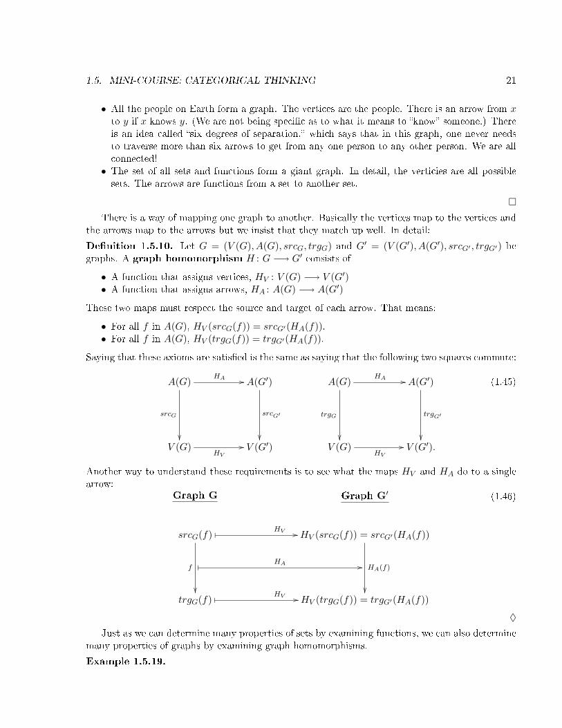
De�nition 1.5.10. Let G = (V (G), A(G), srcG, trgG) and G′ = (V (G′), A(G′), srcG′ , trgG′) begraphs. A graph homomorphism H : G −! G′ consists of

• A function that assigns vertices, HV : V (G) −! V (G′)• A function that assigns arrows, HA : A(G) −! A(G′)

These two maps must respect the source and target of each arrow. That means:

• For all f in A(G), HV (srcG(f)) = srcG′(HA(f)).• For all f in A(G), HV (trgG(f)) = trgG′(HA(f)).

Saying that these axioms are satis�ed is the same as saying that the following two squares commute:

A(G)HA //

srcG

��

A(G′)

srcG′

��

A(G)HA //

trgG

��

A(G′)

trgG′

��V (G)

HV

// V (G′) V (G)HV

// V (G′).

(1.45)

Another way to understand these requirements is to see what the maps HV and HA do to a singlearrow:

Graph G Graph G′

srcG(f)

f

��

� HV // HV (srcG(f)) = srcG′(HA(f))

HA(f)

��

� HA //

trgG(f) � HV // HV (trgG(f)) = trgG′(HA(f))

(1.46)

♦

Just as we can determine many properties of sets by examining functions, we can also determinemany properties of graphs by examining graph homomorphisms.

Example 1.5.19.


• A vertex of a graph G can be described by a graph homomorphism from the one vertex graphH : ∗ −! G.• A directed edge of a graph can be determined by a graph homomorphism from the graph∗ −! ∗ to G.• A triangle in a graph G can be determined by a graph homomorphism from the graph

∗ //

��

∗

��∗

(1.47)

to the graph G.• A path of length n in a graph G can be determined by a graph homomorphism from the�snake� graph

∗ // ∗ // ∗ // · · · // ∗ (1.48)

of length n to G.

�

Exercise 1.5.12. Prove that a graph G is weakly connected (for any two vertices x and y, thereis either a path from x to y or a path from y to x) if there does not exist a surjective (on vertices)graph homomorphism from G to the graph

∗��

∗��

(1.49)

Solution: If G is not weakly connected, then we will be able to split the graph into two partswith no arrow from one to another. Send all the nodes of one graph to one ∗ and all the arrows tothe single arrow. Send all the other objects to the other ∗. If the graph is weakly connected, thenthis partitioning would not be possible.

�

Exercise 1.5.13. Use graph homomorphisms to determine di�erent types of paths in a graph.

1. How do you describe a simple path in a graph (a simple path is a path that does not haverepeated vertices)?

2. What about a cycle of length n (a cycle is a path that starts and ends at the same vertex)?3. Do the same for a simple cycle of length n (a simple cycle is a cycle in which the only repeating

vertex is the starting point which is the ending point).

Solution:

1. One-to-one functions from the �snake� graph, Diagram 1.48, to any graph will correspond tosimple paths.


2. Functions from �ring� graphs of the form

•

��•

??

•

��•

OO

•

��•

__

will describe such cycles.3. One-to-one functions from the �ring� graphs will correspond to simple cycles.

�

Exercise 1.5.14. Show that the composition of graph homomorphisms is a graph homomorphism.Show that the composition is associative.

Solution: Let H : G −! G′ and H ′ : G′ −! G′′ be graph homomorphisms. Then H ′ ◦H : G −!G′′. The fact that H ′ ◦ H preserves the sources of arrows amounts to the commutativity of thefollowing diagram which is assured because each square commutes.

A(G)HA //

srcG

��

A(G′)

srcG′

��

H′A // A(G′′)

srcG′′

��V (G)

HV

// V (G′)H′V

// V (G′′).

A similar argument must be made to show that H ′ ◦H preserves targets. The proof of the associa-tivity of the composition of graph homomorphisms comes from the fact that they are functions andis similar to the solution to Exercise 1.5.9.

�

Exercise 1.5.15. De�ne the identity graph homomorphism, IG, for any graph G. Show thatif H : G −! G′ is a graph homomorphism then H ◦ IG = H and IG′ ◦H = H.

Solution: IG,A(x) = x and IG,V (f) = f . This graph homomorphism preserves the sources andtargets of the arrows for trivial reasons. The fact that it acts like a unit to composition is becauseit is a function.

�


Groups

Another important structure that is based on sets and related to categories is groups. It is nice tosee the de�nition of a group from a function perspective.

First a discussion of operations. We all know what we mean by operations on numbers. If youtake numbers x and y, you can perform the addition operation and get x+ y. You can also performother operations and get x−y or y×x. All these are examples of binary operations. Operations arereally just functions. For a given set, S, a binary operation is a function f : S×S −! S. For twoelements s and s′, we write the value of f as f(s, s′). A unary operation is a function that takesone element of S and outputs one element of S, i.e., f : S −! S. The inverse operation is a unaryoperation that takes x and returns x−1. There are also trinary operations f : S × S × S −! Sand n-ary operations for all natural numbers n

f : S × S × · · · × S︸︷︷︸n times

−! S. (1.50)

If n = 0 then we write the 0-ary product as the set with one element {∗} and a 0-ary operation iswritten as f : {∗} −! S which basically picks out an element of S, which is called a constant. (Wewill see in a few lines that the identity element, e, of a group is an example of a constant.)

Let us put this all together and give the formal de�nition of a group.

De�nition 1.5.11. A group (G, ?, e, ( )−1) is a set G with the following:

• A multiplication operation: a binary operation ? : G×G −! G.• An identity: there is also a special element e in G called the identity of the group, i.e, a 0-aryoperation u : {∗} −! G.• An inverse operation: a unary operation ( )−1 : G −! G

These structures satisfy the following axioms:

1. The multiplication is associative: for all x, y and z, we have (x ? y) ? z = x ? (y ? z).2. The identity acts like a unit of the multiplication (That is, when you multiply numbers, 1

does not change the number. 1× n = n . 1 is a �unit�): for all x, x ? e = x = e ? x.3. The inverse gives the unit: For all x in G, x ? x−1 = e = x−1 ? x

♦

Here are some examples of groups.

Example 1.5.20.

• The additive integers: (Z,+, 0,−). Addition and subtraction are the usual operations.• The additive real numbers: (R,+, 0,−). Addition and subtraction are the usual operations.• The multiplicative positive reals: (R+,×, 1, ( )−1) where R+ are the positive real numbers,

× is multiplication, and the function ( )−1 takes r to 1r .

• Clock arithmetic: ({1, 2, 3, . . . , 11, 12},+, 12,−) where addition and subtraction is goingaround the clock. 12 is the unit because when you add 12 to any number you get backto the original number. Notice that 12 did not play an important role and that this would betrue for any number.• The trivial group: ({0},+, 0,−). This is the world's smallest group. It has only one elementand the operations work as expected.


�

Part of the three axioms of a group can be seen as commutative diagrams in Figures 1.5, 1.6,and 1.7. We write each of the three axioms as commutative diagram and show where the elementsof the sets go outside of the diagrams.

x, y, z � //_

��

x ? y, z_

��

G×G×G ?×id //

id×?

��

G×G

?

��G×G ?

// G

x, y ? z � // x ? (y ? z) = (x ? y) ? z

(1.51)

Figure 1.5: Axiom showing the assoicativity of group multiplication

x_

��

� // x, ∗_

��

G' //

id

��

G× {∗}

id×u

��G G×G?oo

x = x ? e x, e�oo

(1.52)

Figure 1.6: Axiom showing that the identity acts like a unit

Exercise 1.5.16. Diagram 1.6 shows the x = x?e part of the axiom. Give a commutative diagramfor the x = e ? x part of the axiom.

Solution: It is essentially the same diagram but change the G× {∗} to {∗} ×G.�

Exercise 1.5.17. Diagram 1.7 shows the e = x ? x−1 part of the axiom. Give the commutativediagram for the e = x−1 ? x part of the axiom.

Solution: It is essentially the same diagram with the id× ( )−1 map switched to ( )−1 × id.�


x � //_

��

x, x_

��

G∆ //

��

G×G

id×( )−1

��G×G

?

��

x, x−1_

��

{∗} u// G

∗ � // e = x ? x−1.

(1.53)

Figure 1.7: Axiom showing the existence of inverses

Important Categorical Idea 1.5.2 Many times, even when we have a nice, clear de�ni-tion or description of an object in terms of elements, we still desire a description in termsof morphisms. The reason why such a description is important is that once we have it, wecan use the morphism description in many di�erent categories. Whereas a description interms of elements is good only in one context, a description in terms of morphisms can beused in many di�erent categories and contexts. We will see this de�nition of group arisein other contexts besides sets and functions. ©

There is a way of mapping one group to another.

De�nition 1.5.12. Let (G, ?, e, ( )−1) and (G′, ?′, e′, ( )′−1) be groups. A group homomorphism

f : (G, ?, e, ( )−1) −! (G′, ?′, e′, ( )′−1) is a function f : G −! G′ that satis�es the following twoaxioms

• The function respects the group operation: for all x, y ∈ G, f(x ? y) = f(x) ?′ f(y)• The function respects the unit: f(e) = e′

We can write these two requirements as the following two commutative diagrams.

G×Gf×f //

?

��

G′ ×G′

?′

��

{∗}

u

��

u′

��G

f// G′ G

f// G′

(1.54)

♦

Technical Point 1.5.2 We did not insist that f respect inverses. Do not worry about it. It istrue without saying it because it is a consequence of the other two axioms. First notice that in any


group, x−1 is the unique inverse of the element x. To see this, imagine that x has two inverses yand y′. Consider the following sequence of equalities

y = y ? e unit axiom

= y ? (x ? y′) y′ is the inverse of x

= (y ? x) ? y′ associativity axiom

= e ? y′ y is the inverse of x

= y′ unit axiom

This shows that y = y′. Now lets use this fact to show that inverses are preserved by grouphomomorphisms. First consider

e′ = f(e) = f(xx−1) = f(x)f(x−1). (1.55)

This shows that the inverse of f(x) is f(x−1). But since inverses are unique, we proved f(x)−1 =f(x−1). ♥

Example 1.5.21. Here are some examples of group homomorphisms.

• There is always a unique group homomorphism from any group to the trivial group whereevery element of the group goes to e.• There is always a unique group homomorphism from the trivial group to any group in whichthe identity of the trivial group goes to the identity of the group.• There is an inclusion function inc : Z −! R.• There is a group homomorphism Z −! {0, 1, 2, 3, . . . , 11} that takes every whole number xand sends it to the remainder when x is divided by 12.• Let b be some positive real number called the �base�. There is a exponential function

b( ) : (R,+, 0,−) −! (R+,×, 1, ( )−1) (1.56)

that takes a real number r and sends it to br. The two requirements to be a group homo-morphism turn out to mean that br+r

′= br × br′ (it takes addition to multiplication) and

b0 = 1.• There is a logarithm function that is the inverse of the exponential function.

logb : (R+,×, 1, ( )−1) −! (R,+, 0,−). (1.57)

logb takes a positive real number r to logb(r). The requirements to be a group homomorphismare the well-known facts that logb(r × r′) = logb(r) + logb(r

′) and logb(1) = 0.

�

Exercise 1.5.18. Show that the composition of group homomorphisms is a group homomorphism.Show that the composition is associative.

Solution: Let f : G −! G′ and f ′ : G′ −! G′′ be group homomorphisms. Then (f ′ ◦ f)(x) =f ′(f(x)). To show that it preserves the group operations:

(f ′ ◦ f)(x ? x′) = f ′(f(x ? x′) = f ′(f(x) ?′ f(x′)) = f ′(f(x)) ?′′ f ′(f(x′)) = (f ′ ◦ f)(x) ?′′ (f ′ ◦ f)(x′).


And(f ′ ◦ f)(e) = f ′(f(e)) = f ′(e′) = e′′.

.�

Exercise 1.5.19. De�ne the identity group homomorphism, idG, for every group(G, ?, 0, ( )−1). Show that if f : (G, ?, e, ( )−1) −! (G′, ?′, e′, ( )′−1) is a group homomorphismthen f ◦ idG = f and idG′ ◦ f = f .

Solution: The identity trivially respects the group operation and the identity. The last part followsfrom the fact that group homomorphisms are simply functions (that satisfy certain properties.)

�

Further Reading

Most of the material found in this Section can be found in any discrete mathematics or �nitemathematics textbook e.g. [84, 83]. They can also be found in many pre-calculus textbooks.

This idea of showing the centrality of functions between sets was taken from two books coau-thored by one of the leaders of category theory, F. William Lawvere. With Robert Rosebrugh hewrote the very readable Sets for Mathematics [55] and with Stephen H. Schanuel he wrote a veryinteresting textbook titled Conceptual Mathematics [57].

The novice can �nd basic group theory in any introduction to modern algebra or abstract algebra,e.g., [1, 31].

This idea that most of the operations on functions can be seen as compositions, extensions andliftings (as in Diagram 1.40) was taken from [92] where much of category theory is built out of theseoperations. We will see more of extensions and liftings in Section 10.1.

However, if you really want to learn more about categorical thinking, roll up your sleeves andkeep on reading the rest of this book!

Chapter 2

Categories

A good stack of examples, as large as possible, is indispensable for a thorough understanding of anyconcept, and when I want to learn something new, I make it my �rst job to build one.

Paul Halmos

2.1 Basic De�nitions and Examples

Before going on to the formal de�nition of a category, let us summarize what we saw in Section1.5 about sets and functions. The collection of sets and functions form a category. By carefullyexamining this collection, we will see what we want in a de�nition of a category.

Example 2.1.1. Consider the collection of all sets. There are functions between sets. If f is afunction from set S to set T , then we write it as f : S −! T and we call S the domain of f andT the codomain of f . Certain functions can be composed: for f : S −! T and g : T −! U , thereexists a function g ◦f : S −! U which is de�ned for s in S as (g ◦f)(s) = g(f(s)). This compositionoperation is associative. That means that for f : S −! T , g : T −! U and h : U −! V , both waysof associating the functions h ◦ (g ◦ f) and (h ◦ g) ◦ f are equal. In symbols, h ◦ (g ◦ f) = (h ◦ g) ◦ fand on value s of S this function gives the value h(g(f(s))). For every set S there is a functionidS : S −! S which is called the identity function and is de�ned for s in S as idS(s) = s. Theseidentity functions have the following properties: for all f : S −! T , it is true that f ◦ idS = f andidT ◦ f = f . The collection of sets and functions form a category called Set. This category is easyto understand and we will use it to hone our ideas about many structures of category theory. �

Now for the formal de�nition of a category.

De�nition 2.1.1. A category A is a collection of objects, Ob(A), and a collection of morphisms,Mor(A), which has the following structure:

• Every morphism has an object associated to it called its domain: there is a functionDomA : Mor(A) −! Ob(A).• Every morphism has an object associated to it called its codomain: there is a functionCodA : Mor(A) −! Ob(A). We write

f : a −! b or af // b (2.1)

for the fact that DomA(f) = a and CodA(f) = b.

29

30 CHAPTER 2. CATEGORIES

• Adjoining morphisms can be composed: if f : a −! b and g : b −! c, then there is anassociated morphism g ◦ f : a −! c. We write these morphisms as

af //

g◦f

&&b

g // c. (2.2)

• Every object has an identity morphism: there is a function IdentA : Ob(A) −!Mor(A). Thedomain and codomain of the identity morphism for a is a. We denote the identity of a asida : a −! a or

a.

ida

��(2.3)

This structure must satisfy the following two axioms:

1. Composition is associative: given f : a −! b, g : b −! c and h : c −! d, the two ways ofcomposing these maps are equal:

h ◦ (g ◦ f) = (h ◦ g) ◦ f : a −! d. (2.4)

2. Composition with the identity does not change the morphism: for any f : a −! b the compo-sition with ida is f , i.e., f ◦ ida = f and composition with idb is also f , i.e., idb ◦ f = f.

♦

Basic Examples

Example 2.1.2. Let us mention three examples of categories that we already saw in this text.Although we did not call them categories, the examples and exercises showed that they have thestructure of a category.

• Sets and functions between them form the category Set.• Directed graphs and graph homomorphisms give us Graph.• Groups and group homomorphisms make up Group.

�

The de�nition of a category is a �mouthful� that has many parts to it. There are many importantcomments to every part of the de�nition.

• Ob(A) andMor(A) are called �collections� rather than the more set theoretical �set� or �class�.The reason for this is because we do not want to get bogged down in the language of set theory.If you know the language of set theory, then realize that sometimes our categories will havesets as objects. Sometimes proper classes. Sometimes we will not specify which and we justuse the word �collection.�• It is important to notice that if we have morphisms f : a −! b and g : b −! c then we write thecomposition as g ◦ f rather than f ◦ g. We do this because in many categories the morphismswill be types of functions and with functions, when we apply the composition of functions, itlooks like this g(f( )) which is closer to g ◦ f than f ◦ g. As we get more and more used tothe language we will write gf rather than g ◦ f .

2.1. BASIC DEFINITIONS AND EXAMPLES 31

• Another way of seeing the de�nition of a category is to discuss collections of morphisms. Forobjects a and b in category A, there is a collection of all the morphisms from a to b which wewrite HomA(a, b). The word Hom comes from the word �homomorphism� which is a vestigeof the algebraic and topological background of category theory. We call these collections homsets even though the collections might not be a set. Composition in the category in terms ofthe hom sets becomes the operation

◦ : HomA(b, c)×HomA(a, b) // HomA(a, c)

(g, f) � // g ◦ f.

(2.5)

The fact that every element a of A has an identity element means that there is a specialmorphism in HomA(a, a) that satis�es certain properties. As time goes on, and it is obviouswhat category we mean, we will drop the subscript and write Hom(a, b)

The categories Set, Graph andGroup each have collections of objects and morphisms that arein�nite. Let us look at some examples of categories with �nite collections of objects and morphisms.

Example 2.1.3. Figure 2.1 has several �nite categories which will be of interest. In detail,

a

id

��a //

id

��b

id

��

0 1 2

a

id

��b

id

��a

//

id

��b

id

��oo a //

��

id

��b

id

��

��c

id

DD

2◦ 2I 3

Figure 2.1: Several �nite categories.

• 0, the empty category, has no objects and no morphisms. All the axioms of being a categoryare vacuously true.• 1 has one object and the single identity morphism on that object.• 2 has two objects and three morphisms. Two of the morphisms are identity morphisms on thetwo objects and the third morphism goes from one object to the other.

Documents

Monoidal Categories - Computer and Information Sciencenoson/MCbeginning.pdf · monoidal categories, ... category theory we learned can describe an entire eld. ... there is a self-contained