Embed Size (px)
Citation preview
Page 1 of 15
12th National Convention on Statistics (NCS) EDSA Shangri-La Hotel, Mandaluyong City
October 1-2, 2013
MONITORING TV RATINGS USING MULTIVARIATE CONTROL CHARTS FOR TIME SERIES DATA
by
Genelyn Ma. F. Sarte and Jasper Tamargo
For additional information, please contact: Author’s name : Genelyn Ma. F. Sarte Designation : Associate Professor and Director for Undergraduate Studies Affiliation : School of Statistics, University of the Philippines Address : University of the Philippines, Magsaysay Ave., Diliman, Quezon City Tel. no. : +632- 9280881 E-mail : [email protected] Author’s name : Jasper Tamargo Designation : Research Executive Affiliation : Mediacorp, Singapore Address : Singapore E-mail : [email protected]
Page 2 of 15
MONITORING TV RATINGS USING MULTIVARIATE CONTROL CHARTS FOR TIME SERIES DATA
by
Genelyn Ma. F. Sarte1,2 , and Jasper Tamargo3
ABSTRACT
It is not uncommon for data, including time series data, to be naturally multivariate. In process monitoring and control, there are situations when simultaneous monitoring of 2 or more characteristics may be necessary. This situation is true when monitoring TV ratings, which produce autocorrelated data for each program over time, and correlated data across different networks for the same time slot. While it is possible to produce control charts for TV ratings for competing programs individually, this can be misleading since these are correlated. This paper explores the use of Hotelling T2 control chart and the Principal Component – based control chart using TV ratings from 2008 – 2011.
Key words: Hotelling T2 control chart, Principal Component – based control chart, TV ratings
1. Introduction
(Wicks, 2001) noted that people around the globe spend more than 3.5 billion hours watching television each day. Television has become a common entertainment tool in homes, offices, and even in institutions, serving as a vehicle for advertising, and a source of amusement and news. (Gray and Loyz, 2012) concluded that television programs remain broadly shared pieces of culture that challenge, entertain, anger and inform us, and the ideas within them continue to maintain a pervasive hold on how we imagine our worlds. They added that it may be the case that a greater variety of worlds may be on offer, but this is all the more reason to dig in deeply and seek to understand the many roles and reasons that television endures.
Understanding the relationships among producers, networks, stations and advertisers requires same attention to their ultimate customer - the audience. If no one is watching, there is no point in putting on shows. (Walker et. al., 1998) said that it is the attention of a mass audience that the advertisers are trying to distract to their product and services.
TV Ratings. TV viewership is usually measured in terms of ratings and audience share. A rating is defined as the audience in thousands of a period, divided by the universe of the target worked on, while audience share is the proportion of average audience of a channel in percentage contrasted with the audience of total television in percentage. Daytime refers to shows that fall within the time band of 0500h to 1800h, while primetime refers to shows that fall within the time band of 1801h to 2400h. In case a program breaches the borderline, it is considered to fall within the time band where the majority of the program minutes are located.
How are these measured? The peoplemeter as described by (Green, 2010) is essentially a box about the size of a paperback book with a display screen, which sits near or on top of each television set in a sample household. The meter comes with a remote control device, and each member of a household is assigned an individual button which they are asked to press every time they enter or leave a room with the television set on. All the
Page 3 of 15
devices in a home are connected to a central unit which is ‘polled’ by the research company's computer each night through the panel member's landline or mobile phone. If the TV is turned on and no viewer identifies himself, the meter flashes to remind them to press their button. Additional buttons enable guests to register their presence in the household. He pointed out that the issue of statistical accuracy is becoming more important as the average audiences to programs continue to decline.
Control Charts. (Montgomery, 2009) describes a control chart as one of the primary techniques of statistical process control. It is a plot of a process characteristic, usually over time with statistically determined limits. It is a statistical tool used to distinguish between process variation resulting from common causes and variation resulting from special causes. It can be a useful monitoring technique in a way that when unusual sources of variability are present, sample averages of a characteristic will plot outside the control limits. When used for process monitoring, it helps the user to determine the appropriate type of action to take on the process (Yu, 2007). A multivariate control chart is a special case of variables control charts, which plots statistics from more than one related measurement variables. It shows how several variables jointly influence a process or outcome.
This paper illustrates how multivariate control charts may be used for correlated variables which are also autocorrelated. In particular, the principal component analysis (PCA) – based control chart and the Hotelling T2 control chart will be used on TV ratings in Metro Manila. In monitoring daily TV ratings, autocorrelated data are produced for each program over time and the data across different networks for the same time slot are expected to be correlated. The control charts may be possibly used in detecting unusual occurrences that may be due to network programming or failure in the system.
During the period covered by the analysis, the media landscape in the Philippines consists mainly of the Lopez-owned company ABS-CBN, its major competitor GMA 7, the “newest” in the industry TV 5, and the government run NBN channel. This paper will focus only on three networks ABS-CBN, GMA 7 and TV 5. The initial results in this paper are based only on TV ratings for primetime programming on weekdays (Monday to Friday) from January 1, 2008 to November 30, 2011. 2. Univariate and Multivariate Control Charts
The most widely used and popular SPC techniques involve univariate methods, that is, observing and analyzing a single variable at a time (Damarla, 2011). Amongst these tools, Shewhart control chart has been the most technically sophisticated and widely used method to control the central tendency of a process developed by Walter A. Shewhart in the 1920s. The combined investigation of (Salah and Wu, 2009) stated that one major drawback of the Shewhart chart is that it considers only the last data point and does not carry a memory of the previous data. Therefore, small changes in the mean of a random variable are less likely to be detected rapidly. (Montgomery, 2009) defines two effective alternatives to the Shewhart control chart that may be used when small process shifts are of interest: the cumulative sum (cusum) control chart and the exponentially weighted moving average (EWMA) control chart.
The CUSUM. The CUSUM chart as explained in (Montgomery, 2009) plots the cumulative sums of the deviations of the sample values from a target value. Supposing that samples of size n ≥ 1 are collected, and is the average of the jth sample, then if is the
target for the process mean, the CUSUM control chart is formed by plotting the quantity
= - )
Page 4 of 15
against the sample number. is called the cumulative sum up to and including the ith
sample. This further supports his claim that the most practical applications of the CUSUM employ a tabular procedure in which the CUSUM statistic is accumulated as two-sided statistics defined as
= - ( + K) +
= ( - K) - + ]
where = = 0, and the constant K is called the reference value which is usually
selected to be about one-half of the magnitude of the shift.
Although applying univariate control charts to each individual variable is a possible solution, it may be inefficient and may lead to erroneous conclusions. Multivariate methods that consider the variables jointly are required (Montgomery, 2009). (Salah and Wu, 2009) established that multivariate analysis utilize the additional information due to the relationships among the variables and these concepts may be used to develop more efficient control charts than the simultaneous operation of several univariate control charts. Multivariate quality-control (or process-monitoring) problems as defined by (Montgomery, 2009) are those process-monitoring problems in which several related variables are of interest.
The Hotelling Control Chart. From the 2003 Engineering Statistics Handbook,
Hotelling’s is defined as a scalar that combines information from the dispersion and mean
of several variables. Compared to the univariate case, when data are grouped, the chart
can be paired with a chart that displays a measure of variability within the subgroups from all the analyzed characteristics. (Chang, S. I., & Chou, S., 2010) stated that the multivariate
control charts such as Hotelling are often used for a process of multiple quality
characteristics. They figured that the look of a multivariate control chart often mimics that of univariate control chart such as chart consisting of three horizontal lines enclosing dots
connected by straight line segments. (Khalidi, 1998) illustrated that the multivariate process control problem involves a repetitive process in which each characteristic is represented by
random variables, , ,…, . The probability distribution of the process characteristics is
assumed to be a multivariate normal with a mean vector μ and a covariance matrix Σ. Multiple measurements of each process are assumed to be drawn from a population with standard values for and . When changes in the process cause elements of μ or Σ to
shift from the standard values, it is necessary to detect and correct the change to ensure a stable process.
In practice, Montgomery (2009) stated the need to estimate for the analysis
of preliminary samples of size n, taken when the process is assumed to be in control. Suppose that m such samples are available. The sample means and variances are calculated from each sample as usual; that is,
where is the ith observation on the jth quality characteristics in the kth sample. The
covariance between quality characteristic j and quality characteristic h in the kth sample is
Page 5 of 15
The statistics , and are then averaged over all m samples to obtain
The test statistic now is calculated by the formula . Its
ability to detect a shift in the mean vector depends only on the magnitude of the shift, and not in its direction which is also called a directionally invariant control chart. Since from previous studies, the control chart usage has two distinct phases as summarized by (Khalidi, 1998) and (Montgomery, 2009) that is to say that the objective of Phase I is to obtain an in-control set of observations so that control limits can be established for Phase II, which is the
monitoring of future production. The control limits for the control chart in Phase I are
and
In phase II, when the chart is used for monitoring future production, the control limits are as follows:
and
Although the chart is the most popular, easiest to use and interpret method for
handling multivariate process data, and is beginning to be widely accepted by quality engineers and operators, its use also has some limitations (2003 Engineering Statistics Handbook). Unlike the univariate case, the scale of the values displayed on the chart is not
related to the scales of any of the monitored variables. Also, when the statistic exceeds
the upper control limit, the user does not know which particular variables caused the out-of-control signal. With respect to scaling, it’s better to run individual univariate charts together with the multivariate chart. This will help work on the root that might have caused the signal. However, individual univariate charts can’t explain situations that are a result of some problems in the covariance or correlation between the variables. This is why a dispersion chart must be used.
Principal Component Analysis. Principal Component Analysis (PCA) as defined by (Jackson, 1991) is a multivariate technique in which a number of related variables are transformed to (hopefully, a smaller) set of uncorrelated variables. The method of principal components dates back to Karl Pearson in 1901, although the general procedure as we know it today had to wait for Harold Hotelling whose pioneering paper appeared in 1933. This method of principal components is primarily a data-analytic technique that obtains linear transformations of a group of correlated variables such that certain optimal conditions are achieved. It is a technique for reducing the dimensionality of a data set in which there are a large number of interrelated variables, while retaining as much as possible the variation present in the data set. This reduction is achieved by transforming the interrelated variables to a new set of variables, the principal components, which are uncorrelated, and which are ordered so that the first few retain most of the variation present in all of the original variables.
Page 6 of 15
The PCA-based control charts have no firm guidelines about how much variability needs to be explained in order to produce an effective process-monitoring procedure. The scores are used as an empirical reference distribution to establish a control region for the process. The principal components (PCs)do not always provide a clear interpretation of the situation with respect to the original variables, but they are often effective in diagnosing an out-of-control signal, particularly when the PCs have an interpretation in terms of the original variables.
The standard assumptions in SPC are that the observed process values are normally, independently and identically distributed (IID) with fixed mean µ and standard deviation σ when the process is in control. These assumptions, however, are not always valid. The data may not be normally distributed and/or autocorrelated, especially when the data are observed sequentially and the time between samples are short. The presence of autocorrelation has a significant effect on control charts developed using the assumption of independent observations (Haridy and Wu, 2009).
ARIMA Models. (Mun, 2005) gave a clear discussion of ARIMA econometric modeling that takes into account historical data and decomposes it into an Autoregressive (AR) process, where there is a memory of past events; an Integrated (I) process, which accounts for stabilizing or making the data stationary, making it easier to forecast; and a Moving Average (MA) of the forecast errors, such that the longer the historical data, the more accurate the forecasts will be, as it learns over time. ARIMA models therefore have three model parameters, one for the AR (p) process, one for the I(d) process, and one for the MA(q) process, all combined and interacting among each other and recomposed into the ARIMA (p,d,q) model. Detailed discussion of ARIMA modeling may be found in (Wei, 2005).
3. Methodology
Data. The source of the data for this study is Kantar Media or formerly known as TNS Media Research Philippines which officially released its national television audience measurement data on February 2009. The ratings data used are exclusively from audiences of primetime viewing in Metro Manila. Ratings as known to all broadcasters and media practitioners are the media currency of the TV viewing level of a certain channel or spot. The data covers the weekday period from January 1, 2008 until November 30, 2011 for the primetime (1801h to 2400h time band) ratings of Total TV viewing of Metro Manila residents’ breakdown into ABS-CBN, GMA 7, and TV 5.
Procedure. Because TV ratings for each network are autocorrelated, ARIMA modeling is applied first to each network’s primetime rating. When a suitable model is obtained, the residuals of the model will be used in constructing the control charts. For univariate control charts, CUSUM is used, while for multivariate control charts, both Hotelling T2-based and PCA-based control charts are used. To be effective, this procedure must result in an ARIMA model with parameter estimates that are not biased owing to outliers and that are significant. Residuals of such a model should be normally distributed, independent with constant variance (non-normality could result from presence of outliers in time series or non-constant variance). 4. Results and Discussion
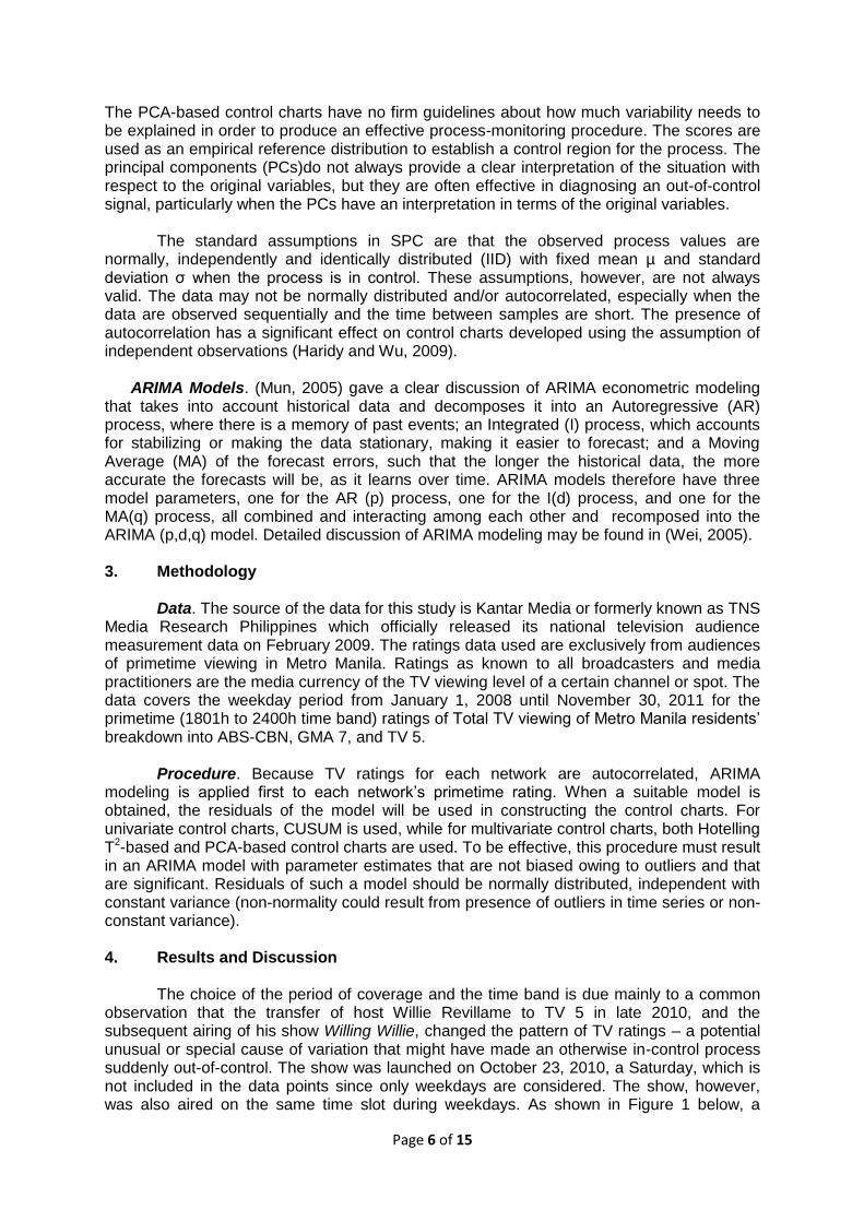
The choice of the period of coverage and the time band is due mainly to a common observation that the transfer of host Willie Revillame to TV 5 in late 2010, and the subsequent airing of his show Willing Willie, changed the pattern of TV ratings – a potential unusual or special cause of variation that might have made an otherwise in-control process suddenly out-of-control. The show was launched on October 23, 2010, a Saturday, which is not included in the data points since only weekdays are considered. The show, however, was also aired on the same time slot during weekdays. As shown in Figure 1 below, a
Page 7 of 15
sudden jump in TV ratings for TV 5 was observed during the last quarter of 2010 that appeared to have reduced the gap between this station’s rating and the ratings of ABS-CBN and GMA 7. This is a 6-hour time band where the show aired for only about two hours. Prior to airing Revillame’s show, TV 5 also never had a rating that breached 10%.
Figure 1. Daily Primetime TV Ratings in Metro Manila
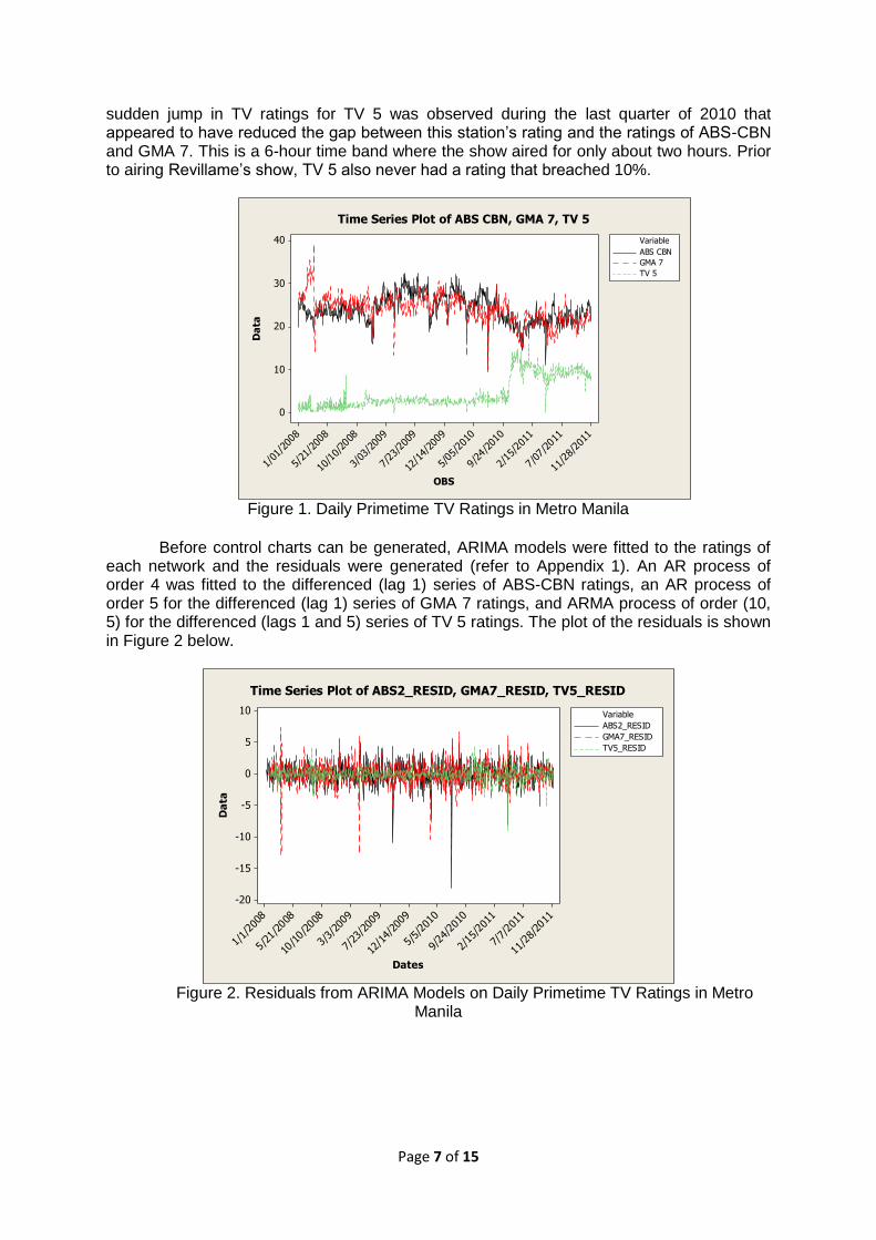
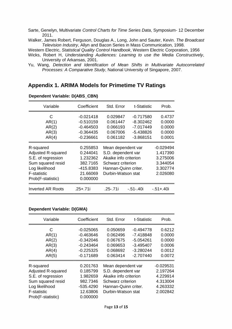
Before control charts can be generated, ARIMA models were fitted to the ratings of each network and the residuals were generated (refer to Appendix 1). An AR process of order 4 was fitted to the differenced (lag 1) series of ABS-CBN ratings, an AR process of order 5 for the differenced (lag 1) series of GMA 7 ratings, and ARMA process of order (10, 5) for the differenced (lags 1 and 5) series of TV 5 ratings. The plot of the residuals is shown in Figure 2 below.
11/2
8/20
11
7/7/20
11
2/15
/201
1
9/24
/201
0
5/5/20
10
12/1
4/20
09
7/23
/200
9
3/3/
2009
10/10/
2008
5/21
/200
8
1/1/20
08
10
5
0
-5
-10
-15
-20
Dates
Da
ta
ABS2_RESID
GMA7_RESID
TV5_RESID
Variable
Time Series Plot of ABS2_RESID, GMA7_RESID, TV5_RESID
Figure 2. Residuals from ARIMA Models on Daily Primetime TV Ratings in Metro
Manila
11/2
8/20
11
7/07
/201
1
2/15
/201
1
9/24
/201
0
5/05
/201
0
12/1
4/20
09
7/23
/200
9
3/03
/200
9
10/1
0/20
08
5/21
/200
8
1/01
/200
8
40
30
20
10
0
OBS
Da
taABS CBN
GMA 7
TV 5
Variable
Time Series Plot of ABS CBN, GMA 7, TV 5
Page 8 of 15
11/1/2
011
6/14
/201
1
1/25
/201
1
9/7/
2010
4/20
/201
0
12/1
/200
9
7/14
/200
9
2/24
/200
9
10/7
/200
8
5/20
/200
8
1/1/
2008
5.0
2.5
0.0
-2.5
-5.0
Dates
Cu
mu
lati
ve
Su
m
0
UCL=5.32
LCL=-5.32
CUSUM Chart of GMA7_RESID
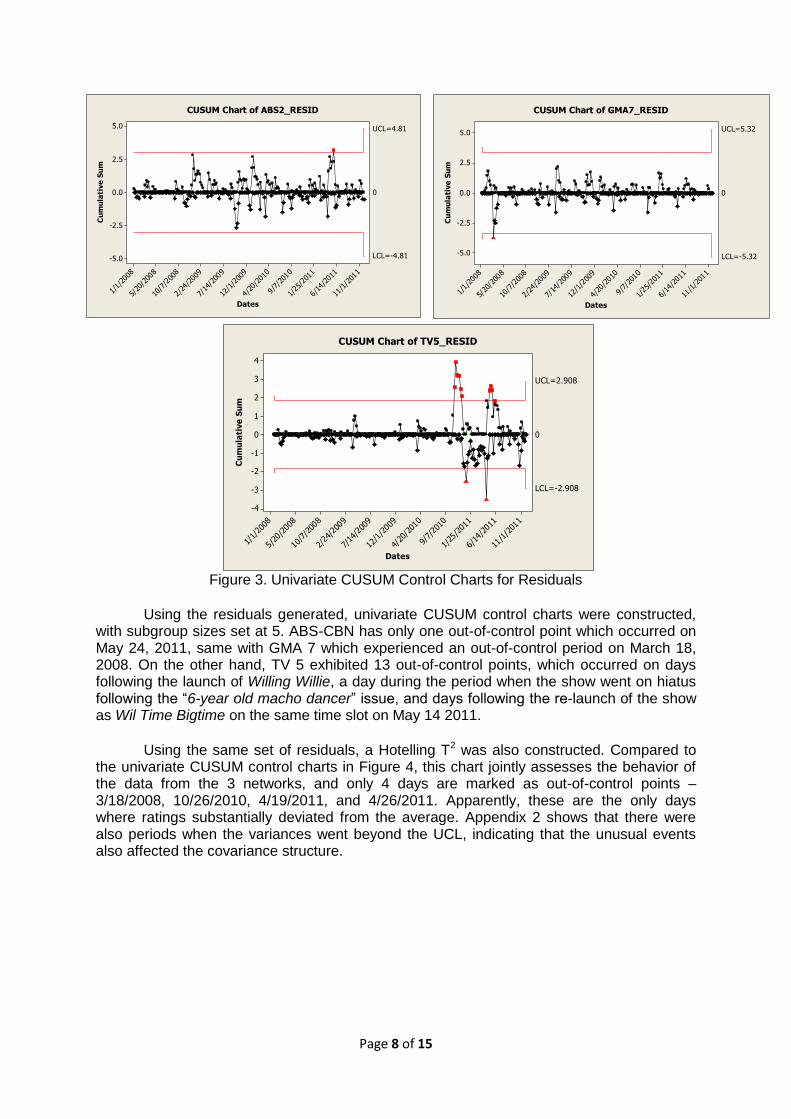
Figure 3. Univariate CUSUM Control Charts for Residuals
Using the residuals generated, univariate CUSUM control charts were constructed, with subgroup sizes set at 5. ABS-CBN has only one out-of-control point which occurred on May 24, 2011, same with GMA 7 which experienced an out-of-control period on March 18, 2008. On the other hand, TV 5 exhibited 13 out-of-control points, which occurred on days following the launch of Willing Willie, a day during the period when the show went on hiatus following the “6-year old macho dancer” issue, and days following the re-launch of the show as Wil Time Bigtime on the same time slot on May 14 2011.
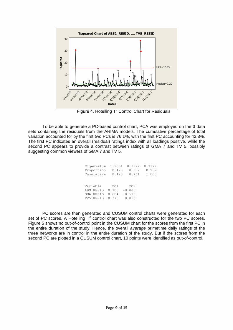
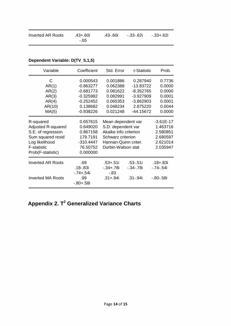
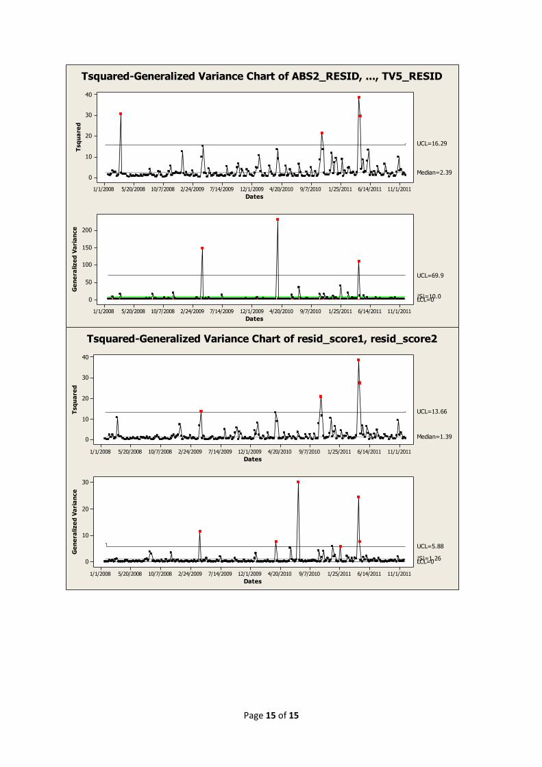
Using the same set of residuals, a Hotelling T2 was also constructed. Compared to the univariate CUSUM control charts in Figure 4, this chart jointly assesses the behavior of the data from the 3 networks, and only 4 days are marked as out-of-control points – 3/18/2008, 10/26/2010, 4/19/2011, and 4/26/2011. Apparently, these are the only days where ratings substantially deviated from the average. Appendix 2 shows that there were also periods when the variances went beyond the UCL, indicating that the unusual events also affected the covariance structure.
11/1
/201
1
6/14
/201
1
1/25
/201
1
9/7/
2010
4/20
/201
0
12/1
/200
9
7/14
/200
9
2/24
/200
9
10/7
/200
8
5/20
/200
8
1/1/
2008
5.0
2.5
0.0
-2.5
-5.0
Dates
Cu
mu
lati
ve
Su
m
0
UCL=4.81
LCL=-4.81
CUSUM Chart of ABS2_RESID
11/1/2
011
6/14
/201
1
1/25
/201
1
9/7/20
10
4/20
/201
0
12/1
/200
9
7/14
/200
9
2/24
/200
9
10/7/2
008
5/20
/200
8
1/1/20
08
4
3
2
1
0
-1
-2
-3
-4
Dates
Cu
mu
lati
ve
Su
m
0
UCL=2.908
LCL=-2.908
CUSUM Chart of TV5_RESID
Page 9 of 15
11/1/2
011
6/14
/201
1
1/25
/201
1
9/7/
2010
4/20
/201
0
12/1
/200
9
7/14
/200
9
2/24
/200
9
10/7
/200
8
5/20
/200
8
1/1/20
08
40
30
20
10
0
Dates
Tsq
ua
red
Median=2.39
UCL=16.29
Tsquared Chart of ABS2_RESID, ..., TV5_RESID
Figure 4. Hotelling T2 Control Chart for Residuals
To be able to generate a PC-based control chart, PCA was employed on the 3 data sets containing the residuals from the ARIMA models. The cumulative percentage of total variation accounted for by the first two PCs is 76.1%, with the first PC accounting for 42.8%. The first PC indicates an overall (residual) ratings index with all loadings positive, while the second PC appears to provide a contrast between ratings of GMA 7 and TV 5, possibly suggesting common viewers of GMA 7 and TV 5.
Eigenvalue 1.2851 0.9972 0.7177
Proportion 0.428 0.332 0.239
Cumulative 0.428 0.761 1.000
Variable PC1 PC2
ABS_RESID 0.705 -0.005
GMA_RESID 0.604 -0.518
TV5_RESID 0.370 0.855
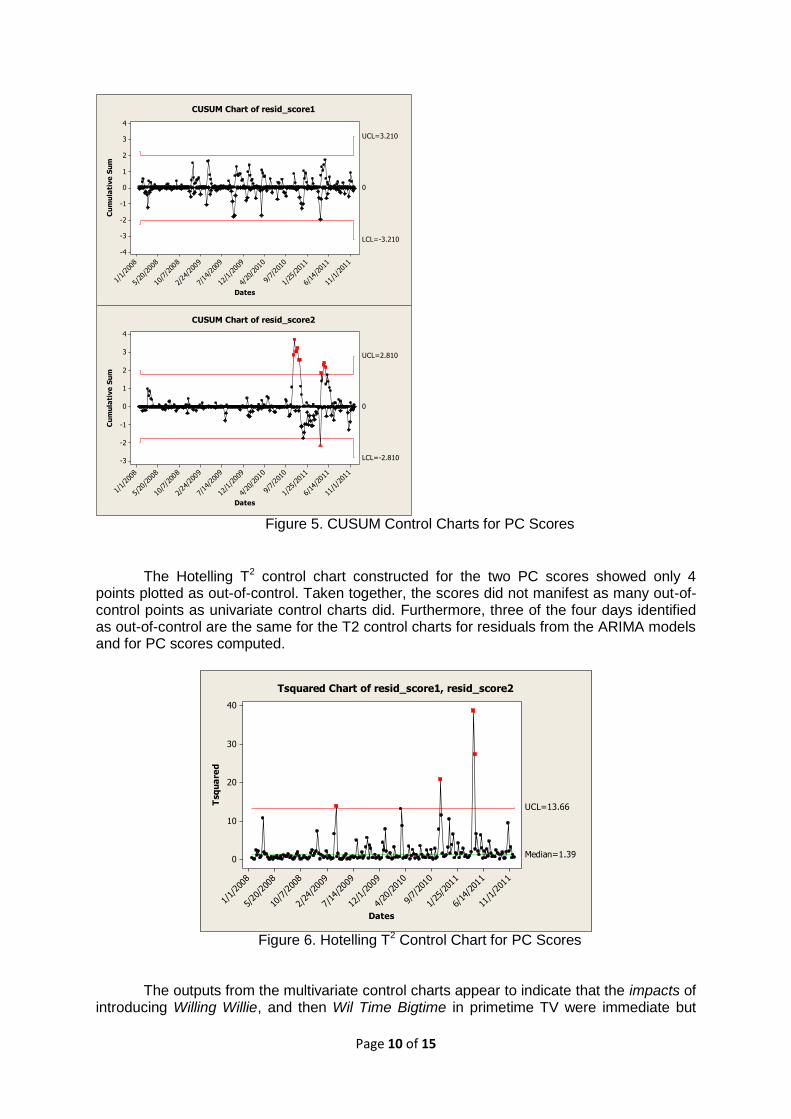
PC scores are then generated and CUSUM control charts were generated for each set of PC scores. A Hotelling T2 control chart was also constructed for the two PC scores. Figure 5 shows no out-of-control point in the CUSUM chart for the scores from the first PC in the entire duration of the study. Hence, the overall average primetime daily ratings of the three networks are in control in the entire duration of the study. But if the scores from the second PC are plotted in a CUSUM control chart, 10 points were identified as out-of-control.
Page 10 of 15
11/1/2
011
6/14
/201
1
1/25
/201
1
9/7/20
10
4/20
/201
0
12/1
/200
9
7/14
/200
9
2/24
/200
9
10/7/2
008
5/20
/200
8
1/1/20
08
4
3
2
1
0
-1
-2
-3
-4
Dates
Cu
mu
lati
ve
Su
m
0
UCL=3.210
LCL=-3.210
CUSUM Chart of resid_score1
11/1/2
011
6/14
/201
1
1/25
/201
1
9/7/20
10
4/20
/201
0
12/1
/200
9
7/14
/200
9
2/24
/200
9
10/7/2
008
5/20
/200
8
1/1/20
08
4
3
2
1
0
-1
-2
-3
Dates
Cu
mu
lati
ve
Su
m
0
UCL=2.810
LCL=-2.810
CUSUM Chart of resid_score2
Figure 5. CUSUM Control Charts for PC Scores
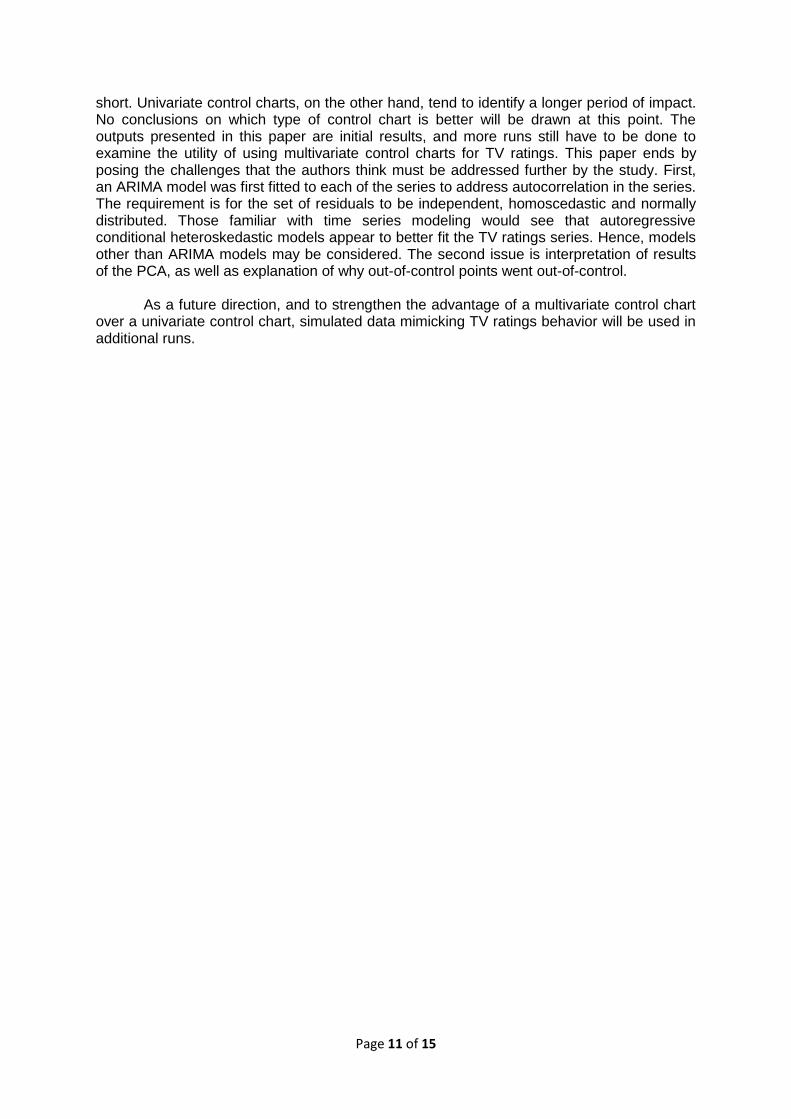
The Hotelling T2 control chart constructed for the two PC scores showed only 4 points plotted as out-of-control. Taken together, the scores did not manifest as many out-of-control points as univariate control charts did. Furthermore, three of the four days identified as out-of-control are the same for the T2 control charts for residuals from the ARIMA models and for PC scores computed.
11/1/2
011
6/14
/201
1
1/25
/201
1
9/7/
2010
4/20
/201
0
12/1
/200
9
7/14
/200
9
2/24
/200
9
10/7
/200
8
5/20
/200
8
1/1/20
08
40
30
20
10
0
Dates
Tsq
ua
red
Median=1.39
UCL=13.66
Tsquared Chart of resid_score1, resid_score2
Figure 6. Hotelling T2 Control Chart for PC Scores
The outputs from the multivariate control charts appear to indicate that the impacts of
introducing Willing Willie, and then Wil Time Bigtime in primetime TV were immediate but
Page 11 of 15
short. Univariate control charts, on the other hand, tend to identify a longer period of impact. No conclusions on which type of control chart is better will be drawn at this point. The outputs presented in this paper are initial results, and more runs still have to be done to examine the utility of using multivariate control charts for TV ratings. This paper ends by posing the challenges that the authors think must be addressed further by the study. First, an ARIMA model was first fitted to each of the series to address autocorrelation in the series. The requirement is for the set of residuals to be independent, homoscedastic and normally distributed. Those familiar with time series modeling would see that autoregressive conditional heteroskedastic models appear to better fit the TV ratings series. Hence, models other than ARIMA models may be considered. The second issue is interpretation of results of the PCA, as well as explanation of why out-of-control points went out-of-control.
As a future direction, and to strengthen the advantage of a multivariate control chart over a univariate control chart, simulated data mimicking TV ratings behavior will be used in additional runs.
Page 12 of 15
REFERENCES Ang, Ien, Desperately Seeking the Audience, Routledge, 1990. Barwise, Patrick T. and Ehrenberg, Andrew S. C., Television and Its Audience, SAGE
Publications, 1987. Bersimis, Sotiris, et al, Multivariate Statistical Process Control Charts: An Overview, John
Wiley & Sons, Ltd, 2006. Chang, Shing I., and Chou, Shih-Hsiung, A visualization decision support tool for multivariate
SPC diagnosis using marginal CUSUM glyphs, Quality Engineering, p182-198, 2010. Damarla, Seshu Kumar, Multivariate Statistical Process Monitoring and Control, 2011. Engineering Statistics Handbook, NIST/ SEMATECH e-handbook of Statistical Methods,
http://www.itl.nist.gov/div898/handbook/,2003. Farris, Paul , Bendle, Neil , Pfeifer, Phillip , & Reibstein, David, , Marketing metrics: The
definitive Guide to Measuring Marketing Performance, Pearson Education, 2nd Edition, pp XV, pp 2-3. , 2010
Fernando, Mark Phillip C., The Late-Night Effect: Late-Night Television’s Effect on the perception of Political Figures, Georgetown University, 2003.
Gensch, Dennis and Shaman, Paul, Models of Competitive Television Ratings, Journal of Marketing Research, XVII, 1980, pp 307-315.
Gray, Jonathan and Lotz, Amanda D., Television Studies, Polity, 2012, pp 145. Green, Andre, From Prime Time to My Time – Measuring Television Audiences, Warc, 2010. Hair, Joseph F. Jr., Black, William C., Babin, Barry J., and Anderson, Rolph E., Multivariate
Data Analysis, ISBN-10, Prentice Hall, Pearson International Edition, pp 16-24 , 6th – 7th Edition, 2010.
Haridy, Salah and Wu, Zhang, Univariate and Multivariate Control Charts for Monitoring Dynamic-behavior Processes: A Case Study, Journal of Industrial Engineering and Management, 2009.
Henry, Michael D. and Rinne, Heikki J., Predicting Program Shares in New Time Slots, Journal of Advertising Research, 1984, pp 9-17.
Horen, Jeffrey H., Scheduling of Network Television Programs, Management Science, 1980, 26(4), pp 354-370.
Jackson, J. Edward, A user’s Guide to Principal Components, Wiley-Interscience, 1991. Johnson , Richard and Wichern, Dean W, Applied Multivariate Statistical Analysis, Pearson,
6th Edition, 2007. Kantar Media Philippines, Television Viewing Level, Infosys+, Quezon City, Kantar Media
Philippines, 25 July 2011. Lu Xiaoling, Modelling of Television Audience viewing Behavior, City University of Hong
Kong, 2007. Mohammad, Said Asem Khalidi, Multivariate Quality Control: Statistical Performance and
Economic Feasibility, Wichita State University, 1998. Montgomery, Douglas C., Introduction to Statistical Quality Control, New York, John Wiley &
Sons, 6th Edition, 2009. Mun, Jonathan, Real Options Analysis: Tools and Techniques for Valuing Strategic
Investments and Decisions, John Wiley & Sons, 2002. Napoli, Philip M., The Unpredictable Audience: An Exploratory Analysis of Forecasting Error
for New Prime-Time Network Television Programs, Journal of Advertising, 2001, 30(2), pp 53-60.
Noskievicová, Darja, Control Chart Limits Setting when Data are Auto-Correlated, 10th QMOD Conference - Quality Management and Organiqatinal Development. Our Dreams of Excellence, Sweden, 18-20 June 2007.
Psarakis S. and Papaleonida G.E.A, SPC Procedures for Monitoring Autocorrelated Processes, Quality Technology and Quantitative Management Vol 4, No.4, pp. 501-54-, 2007
Roberto, Eduardo, Applied Marketing Research: For data-based Marketing decisions, Ateneo de Manila University Press, 1987.
Page 13 of 15
Sarte, Genelyn, Multivariate Control Charts for Time Series Data, Symposium- 12 December 2011.
Walker, James Robert, Ferguson, Douglas A., Long, John and Sauter, Kevin. The Broadcast Television Industry, Allyn and Bacon Series in Mass Communication, 1998.
Western Electric, Statistical Quality Control Handbook, Western Electric Corporation, 1956 Wicks, Robert H, Understanding Audiences: Learning to use the Media Constructively,
University of Arkansas, 2001. Yu, Wang, Detection and Identification of Mean Shifts in Multivariate Autocorrelated
Processes: A Comparative Study, National University of Singapore, 2007.
Appendix 1. ARIMA Models for Primetime TV Ratings
Dependent Variable: D(ABS_CBN) Variable Coefficient Std. Error t-Statistic Prob. C -0.021418 0.029847 -0.717580 0.4737
AR(1) -0.510159 0.061447 -8.302462 0.0000
AR(2) -0.464503 0.066193 -7.017449 0.0000
AR(3) -0.364435 0.067006 -5.438826 0.0000
AR(4) -0.236661 0.061182 -3.868151 0.0001 R-squared 0.255853 Mean dependent var -0.029494
Adjusted R-squared 0.244041 S.D. dependent var 1.417390
S.E. of regression 1.232362 Akaike info criterion 3.275006
Sum squared resid 382.7165 Schwarz criterion 3.344054
Log likelihood -415.8383 Hannan-Quinn criter. 3.302774
F-statistic 21.66069 Durbin-Watson stat 2.026080
Prob(F-statistic) 0.000000 Inverted AR Roots .25+.71i .25-.71i -.51-.40i -.51+.40i
Dependent Variable: D(GMA) Variable Coefficient Std. Error t-Statistic Prob. C -0.025065 0.050659 -0.494778 0.6212
AR(1) -0.463646 0.062496 -7.418848 0.0000
AR(2) -0.342046 0.067675 -5.054261 0.0000
AR(3) -0.243464 0.069653 -3.495407 0.0006
AR(4) -0.225325 0.068692 -3.280244 0.0012
AR(5) -0.171689 0.063414 -2.707440 0.0072 R-squared 0.201763 Mean dependent var -0.029531
Adjusted R-squared 0.185799 S.D. dependent var 2.197264
S.E. of regression 1.982659 Akaike info criterion 4.229914
Sum squared resid 982.7346 Schwarz criterion 4.313004
Log likelihood -535.4290 Hannan-Quinn criter. 4.263332
F-statistic 12.63806 Durbin-Watson stat 2.002842
Prob(F-statistic) 0.000000
Page 14 of 15
Inverted AR Roots .43+.60i .43-.60i -.33-.62i -.33+.62i
-.65
Dependent Variable: D(TV_5,1,5) Variable Coefficient Std. Error t-Statistic Prob. C 0.000543 0.001886 0.287940 0.7736
AR(1) -0.863277 0.062388 -13.83722 0.0000
AR(2) -0.681773 0.081622 -8.352765 0.0000
AR(3) -0.325982 0.082991 -3.927909 0.0001
AR(4) -0.252452 0.065353 -3.862903 0.0001
AR(10) 0.138682 0.048234 2.875220 0.0044
MA(5) -0.938226 0.021248 -44.15672 0.0000 R-squared 0.657615 Mean dependent var -3.61E-17
Adjusted R-squared 0.649020 S.D. dependent var 1.463716
S.E. of regression 0.867158 Akaike info criterion 2.580851
Sum squared resid 179.7191 Schwarz criterion 2.680597
Log likelihood -310.4447 Hannan-Quinn criter. 2.621014
F-statistic 76.50752 Durbin-Watson stat 2.035947
Prob(F-statistic) 0.000000 Inverted AR Roots .69 .53+.51i .53-.51i .18+.83i
.18-.83i -.34+.78i -.34-.78i -.74-.54i
-.74+.54i -.83
Inverted MA Roots .99 .31+.94i .31-.94i -.80-.58i
-.80+.58i
Appendix 2. T2 Generalized Variance Charts
Page 15 of 15
11/1/20116/14/20111/25/20119/7/20104/20/201012/1/20097/14/20092/24/200910/7/20085/20/20081/1/2008
40
30
20
10
0
Dates
Tsq
ua
red
Median=2.39
UCL=16.29
11/1/20116/14/20111/25/20119/7/20104/20/201012/1/20097/14/20092/24/200910/7/20085/20/20081/1/2008
200
150
100
50
0
Dates
Ge
ne
ralize
d V
ari
an
ce
|S|=10.0
UCL=69.9
LCL=0
Tsquared-Generalized Variance Chart of ABS2_RESID, ..., TV5_RESID
11/1/20116/14/20111/25/20119/7/20104/20/201012/1/20097/14/20092/24/200910/7/20085/20/20081/1/2008
40
30
20
10
0
Dates
Tsq
ua
red
Median=1.39
UCL=13.66
11/1/20116/14/20111/25/20119/7/20104/20/201012/1/20097/14/20092/24/200910/7/20085/20/20081/1/2008
30
20
10
0
Dates
Ge
ne
ralize
d V
ari
an
ce
|S|=1.26
UCL=5.88
LCL=0
Tsquared-Generalized Variance Chart of resid_score1, resid_score2