Embed Size (px)
Citation preview

MONITORING THE COEFFICIENT OFVARIATION USING EWMA CHARTS
Philippe CASTAGLIOLA 1, Giovanni CELANO 2, Stelios PSARAKIS 3
1Universite de Nantes & IRCCyN UMR CNRS 6597, France2Universita di Catania, Catania, Italy
3Athens University of Economics and Business, Athens, Greece
ISSPC 2011, July 13–14, Rio de Janeiro, Brazil
Philippe CASTAGLIOLA , Giovanni CELANO , Stelios PSARAKIS MONITORING THE COEFFICIENT OF VARIATION USING EWMA CHARTS

Coefficient of variation
Philippe CASTAGLIOLA , Giovanni CELANO , Stelios PSARAKIS MONITORING THE COEFFICIENT OF VARIATION USING EWMA CHARTS

Coefficient of variation
Definition
Philippe CASTAGLIOLA , Giovanni CELANO , Stelios PSARAKIS MONITORING THE COEFFICIENT OF VARIATION USING EWMA CHARTS

Coefficient of variation
Definition
If X > 0 is a random variable with mean µ and standard-deviation σ, bydefinition the coefficient of variation γ is defined as
γ =σ
µ
Philippe CASTAGLIOLA , Giovanni CELANO , Stelios PSARAKIS MONITORING THE COEFFICIENT OF VARIATION USING EWMA CHARTS

Coefficient of variation
Definition
If X > 0 is a random variable with mean µ and standard-deviation σ, bydefinition the coefficient of variation γ is defined as
γ =σ
µ
Used to compare data sets having different units or widely different means(ex : finance, chemical and biological assays, materials engineering).
Sample coefficient of variation
If {X1, . . . ,Xn} is a sample of n normal i.i.d. (µ, σ) random variablesthen a “natural” estimator of γ is
γ =S
X
where
Philippe CASTAGLIOLA , Giovanni CELANO , Stelios PSARAKIS MONITORING THE COEFFICIENT OF VARIATION USING EWMA CHARTS

Coefficient of variation
Definition
If X > 0 is a random variable with mean µ and standard-deviation σ, bydefinition the coefficient of variation γ is defined as
γ =σ
µ
Used to compare data sets having different units or widely different means(ex : finance, chemical and biological assays, materials engineering).
Sample coefficient of variation
If {X1, . . . ,Xn} is a sample of n normal i.i.d. (µ, σ) random variablesthen a “natural” estimator of γ is
γ =S
X
where X =1
n
n∑
i=1
Xi
Philippe CASTAGLIOLA , Giovanni CELANO , Stelios PSARAKIS MONITORING THE COEFFICIENT OF VARIATION USING EWMA CHARTS
Coefficient of variation
Definition
If X > 0 is a random variable with mean µ and standard-deviation σ, bydefinition the coefficient of variation γ is defined as
γ =σ
µ
Used to compare data sets having different units or widely different means(ex : finance, chemical and biological assays, materials engineering).
Sample coefficient of variation
If {X1, . . . ,Xn} is a sample of n normal i.i.d. (µ, σ) random variablesthen a “natural” estimator of γ is
γ =S
X
where X =1
n
n∑
i=1
Xi and S =
√
√
√
√
1
n − 1
n∑
i=1
(Xi − X )2
Philippe CASTAGLIOLA , Giovanni CELANO , Stelios PSARAKIS MONITORING THE COEFFICIENT OF VARIATION USING EWMA CHARTS

Basic properties of the sample coefficient of variation
Philippe CASTAGLIOLA , Giovanni CELANO , Stelios PSARAKIS MONITORING THE COEFFICIENT OF VARIATION USING EWMA CHARTS

Basic properties of the sample coefficient of variation
c.d.f and inverse c.d.f. of γ
Philippe CASTAGLIOLA , Giovanni CELANO , Stelios PSARAKIS MONITORING THE COEFFICIENT OF VARIATION USING EWMA CHARTS

Basic properties of the sample coefficient of variation
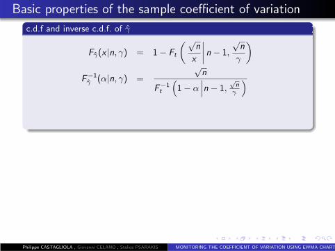
c.d.f and inverse c.d.f. of γ
Fγ(x |n, γ) = 1 − Ft
(√n
x
∣
∣
∣
∣
n − 1,
√n
γ
)
Philippe CASTAGLIOLA , Giovanni CELANO , Stelios PSARAKIS MONITORING THE COEFFICIENT OF VARIATION USING EWMA CHARTS
Basic properties of the sample coefficient of variation
c.d.f and inverse c.d.f. of γ
Fγ(x |n, γ) = 1 − Ft
(√n
x
∣
∣
∣
∣
n − 1,
√n
γ
)
F−1γ (α|n, γ) =
√n
F−1t
(
1 − α∣
∣
∣n − 1,√
n
γ
)
Philippe CASTAGLIOLA , Giovanni CELANO , Stelios PSARAKIS MONITORING THE COEFFICIENT OF VARIATION USING EWMA CHARTS

Basic properties of the sample coefficient of variation
c.d.f and inverse c.d.f. of γ
Fγ(x |n, γ) = 1 − Ft
(√n
x
∣
∣
∣
∣
n − 1,
√n
γ
)
F−1γ (α|n, γ) =
√n
F−1t
(
1 − α∣
∣
∣n − 1,√
n
γ
)
where Ft(.) and F−1t (.) are the c.d.f. and the inverse c.d.f. of the
noncentral t distribution.
c.d.f and inverse c.d.f. of γ2
Philippe CASTAGLIOLA , Giovanni CELANO , Stelios PSARAKIS MONITORING THE COEFFICIENT OF VARIATION USING EWMA CHARTS

Basic properties of the sample coefficient of variation
c.d.f and inverse c.d.f. of γ
Fγ(x |n, γ) = 1 − Ft
(√n
x
∣
∣
∣
∣
n − 1,
√n
γ
)
F−1γ (α|n, γ) =
√n
F−1t
(
1 − α∣
∣
∣n − 1,√
n
γ
)
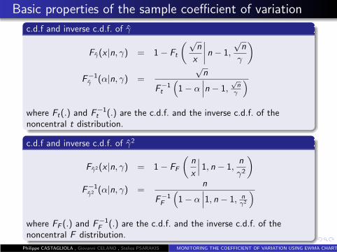
where Ft(.) and F−1t (.) are the c.d.f. and the inverse c.d.f. of the
noncentral t distribution.
c.d.f and inverse c.d.f. of γ2
Fγ2(x |n, γ) = 1 − FF
(
n
x
∣
∣
∣ 1, n − 1,n
γ2
)
Philippe CASTAGLIOLA , Giovanni CELANO , Stelios PSARAKIS MONITORING THE COEFFICIENT OF VARIATION USING EWMA CHARTS

Basic properties of the sample coefficient of variation
c.d.f and inverse c.d.f. of γ
Fγ(x |n, γ) = 1 − Ft
(√n
x
∣
∣
∣
∣
n − 1,
√n
γ
)
F−1γ (α|n, γ) =
√n
F−1t
(
1 − α∣
∣
∣n − 1,√
n
γ
)
where Ft(.) and F−1t (.) are the c.d.f. and the inverse c.d.f. of the
noncentral t distribution.
c.d.f and inverse c.d.f. of γ2
Fγ2(x |n, γ) = 1 − FF
(
n
x
∣
∣
∣ 1, n − 1,n
γ2
)
F−1γ2 (α|n, γ) =
n
F−1F
(
1 − α∣
∣
∣1, n − 1, nγ2
)
Philippe CASTAGLIOLA , Giovanni CELANO , Stelios PSARAKIS MONITORING THE COEFFICIENT OF VARIATION USING EWMA CHARTS
Basic properties of the sample coefficient of variation
c.d.f and inverse c.d.f. of γ
Fγ(x |n, γ) = 1 − Ft
(√n
x
∣
∣
∣
∣
n − 1,
√n
γ
)
F−1γ (α|n, γ) =
√n
F−1t
(
1 − α∣
∣
∣n − 1,√
n
γ
)
where Ft(.) and F−1t (.) are the c.d.f. and the inverse c.d.f. of the
noncentral t distribution.
c.d.f and inverse c.d.f. of γ2
Fγ2(x |n, γ) = 1 − FF
(
n
x
∣
∣
∣ 1, n − 1,n
γ2
)
F−1γ2 (α|n, γ) =
n
F−1F
(
1 − α∣
∣
∣1, n − 1, nγ2
)
where FF (.) and F−1F (.) are the c.d.f. and the inverse c.d.f. of the
noncentral F distribution.
Philippe CASTAGLIOLA , Giovanni CELANO , Stelios PSARAKIS MONITORING THE COEFFICIENT OF VARIATION USING EWMA CHARTS

SH-γ chart (Kang et al., JQT 2007)
Philippe CASTAGLIOLA , Giovanni CELANO , Stelios PSARAKIS MONITORING THE COEFFICIENT OF VARIATION USING EWMA CHARTS

SH-γ chart (Kang et al., JQT 2007)
General assumptions
Philippe CASTAGLIOLA , Giovanni CELANO , Stelios PSARAKIS MONITORING THE COEFFICIENT OF VARIATION USING EWMA CHARTS

SH-γ chart (Kang et al., JQT 2007)
General assumptions
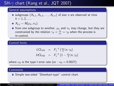
subgroups {Xk,1,Xk,2, . . . ,Xk,n} of size n are observed at timek = 1, 2, . . ..
Philippe CASTAGLIOLA , Giovanni CELANO , Stelios PSARAKIS MONITORING THE COEFFICIENT OF VARIATION USING EWMA CHARTS

SH-γ chart (Kang et al., JQT 2007)
General assumptions
subgroups {Xk,1,Xk,2, . . . ,Xk,n} of size n are observed at timek = 1, 2, . . ..
Xk,j ∼ N(µk , σk).
Philippe CASTAGLIOLA , Giovanni CELANO , Stelios PSARAKIS MONITORING THE COEFFICIENT OF VARIATION USING EWMA CHARTS

SH-γ chart (Kang et al., JQT 2007)
General assumptions
subgroups {Xk,1,Xk,2, . . . ,Xk,n} of size n are observed at timek = 1, 2, . . ..
Xk,j ∼ N(µk , σk).
from one subgroup to another, µk and σk may change, but they areconstrained by the relation γk = σk
µk= γ0 when the process is
in-control.
Control limits
LCLSH = F−1γ
(
α0
2 |n, γ0
)
UCLSH = F−1γ
(
1 − α0
2 |n, γ0
)
where α0 is the type I error rate (ex : α0 = 0.0027).
Comments
Philippe CASTAGLIOLA , Giovanni CELANO , Stelios PSARAKIS MONITORING THE COEFFICIENT OF VARIATION USING EWMA CHARTS
SH-γ chart (Kang et al., JQT 2007)
General assumptions
subgroups {Xk,1,Xk,2, . . . ,Xk,n} of size n are observed at timek = 1, 2, . . ..
Xk,j ∼ N(µk , σk).
from one subgroup to another, µk and σk may change, but they areconstrained by the relation γk = σk
µk= γ0 when the process is
in-control.
Control limits
LCLSH = F−1γ
(
α0
2 |n, γ0
)
UCLSH = F−1γ
(
1 − α0
2 |n, γ0
)
where α0 is the type I error rate (ex : α0 = 0.0027).
Comments
Simple two-sided “Shewhart-type” control chart.
Philippe CASTAGLIOLA , Giovanni CELANO , Stelios PSARAKIS MONITORING THE COEFFICIENT OF VARIATION USING EWMA CHARTS

SH-γ chart (Kang et al., JQT 2007)
General assumptions
subgroups {Xk,1,Xk,2, . . . ,Xk,n} of size n are observed at timek = 1, 2, . . ..
Xk,j ∼ N(µk , σk).
from one subgroup to another, µk and σk may change, but they areconstrained by the relation γk = σk
µk= γ0 when the process is
in-control.
Control limits
LCLSH = F−1γ
(
α0
2 |n, γ0
)
UCLSH = F−1γ
(
1 − α0
2 |n, γ0
)
where α0 is the type I error rate (ex : α0 = 0.0027).
Comments
Simple two-sided “Shewhart-type” control chart.
Unefficient for detecting small change in γ.
Philippe CASTAGLIOLA , Giovanni CELANO , Stelios PSARAKIS MONITORING THE COEFFICIENT OF VARIATION USING EWMA CHARTS

EWMA-γ chart (Hong et al., JSKISE 2008)
Philippe CASTAGLIOLA , Giovanni CELANO , Stelios PSARAKIS MONITORING THE COEFFICIENT OF VARIATION USING EWMA CHARTS

EWMA-γ chart (Hong et al., JSKISE 2008)Monitored statistic
Philippe CASTAGLIOLA , Giovanni CELANO , Stelios PSARAKIS MONITORING THE COEFFICIENT OF VARIATION USING EWMA CHARTS

EWMA-γ chart (Hong et al., JSKISE 2008)Monitored statistic
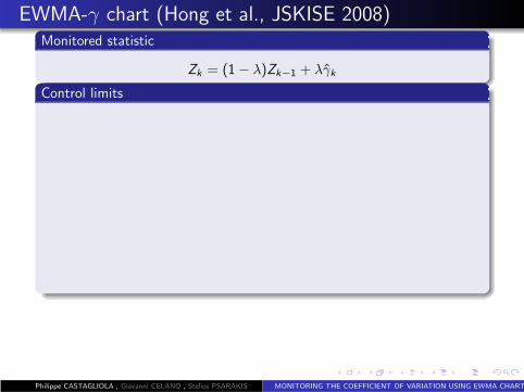
Zk = (1 − λ)Zk−1 + λγk
Philippe CASTAGLIOLA , Giovanni CELANO , Stelios PSARAKIS MONITORING THE COEFFICIENT OF VARIATION USING EWMA CHARTS
EWMA-γ chart (Hong et al., JSKISE 2008)Monitored statistic
Zk = (1 − λ)Zk−1 + λγk
Control limits
Philippe CASTAGLIOLA , Giovanni CELANO , Stelios PSARAKIS MONITORING THE COEFFICIENT OF VARIATION USING EWMA CHARTS

EWMA-γ chart (Hong et al., JSKISE 2008)Monitored statistic
Zk = (1 − λ)Zk−1 + λγk
Control limits
LCLEWMA−γ = µ0(γ) − K
√
λ(1 − (1 − λ)2k )
2 − λσ0(γ)
UCLEWMA−γ = µ0(γ) + K
√
λ(1 − (1 − λ)2k )
2 − λσ0(γ)
Approximations for µ0(γ) and σ0(γ)
µ0(γ) ≃ γ0
(
1 +1
n
(
γ20 −
1
4
)
+1
n2
(
3γ40 −
γ20
4−
7
32
)
+1
n3
(
15γ60 −
3γ40
4−
7γ20
32−
19
128
))
σ0(γ) ≃ γ0
√
1
n
(
γ20 +
1
2
)
+1
n2
(
8γ40 + γ2
0 +3
8
)
+1
n3
(
69γ60 +
7γ40
2+
3γ20
4+
3
16
)
Comments
More efficient than the SH-γ chart.
The paper itself does not provide any thorough investigations(results obtained through simulation only).
Philippe CASTAGLIOLA , Giovanni CELANO , Stelios PSARAKIS MONITORING THE COEFFICIENT OF VARIATION USING EWMA CHARTS

New one-sided EWMA-γ2 charts
Philippe CASTAGLIOLA , Giovanni CELANO , Stelios PSARAKIS MONITORING THE COEFFICIENT OF VARIATION USING EWMA CHARTS

New one-sided EWMA-γ2 chartsWe suggest to ...
Philippe CASTAGLIOLA , Giovanni CELANO , Stelios PSARAKIS MONITORING THE COEFFICIENT OF VARIATION USING EWMA CHARTS

New one-sided EWMA-γ2 chartsWe suggest to ...
1 monitor γ2 instead of γ
Philippe CASTAGLIOLA , Giovanni CELANO , Stelios PSARAKIS MONITORING THE COEFFICIENT OF VARIATION USING EWMA CHARTS
New one-sided EWMA-γ2 chartsWe suggest to ...
1 monitor γ2 instead of γ (more efficient to monitor S2 than S).
Philippe CASTAGLIOLA , Giovanni CELANO , Stelios PSARAKIS MONITORING THE COEFFICIENT OF VARIATION USING EWMA CHARTS
New one-sided EWMA-γ2 chartsWe suggest to ...
1 monitor γ2 instead of γ (more efficient to monitor S2 than S).
2 define 2 EWMA one-sided charts
Philippe CASTAGLIOLA , Giovanni CELANO , Stelios PSARAKIS MONITORING THE COEFFICIENT OF VARIATION USING EWMA CHARTS

New one-sided EWMA-γ2 chartsWe suggest to ...
1 monitor γ2 instead of γ (more efficient to monitor S2 than S).
2 define 2 EWMA one-sided charts (detect shifts more efficiently).
Philippe CASTAGLIOLA , Giovanni CELANO , Stelios PSARAKIS MONITORING THE COEFFICIENT OF VARIATION USING EWMA CHARTS

New one-sided EWMA-γ2 chartsWe suggest to ...
1 monitor γ2 instead of γ (more efficient to monitor S2 than S).
2 define 2 EWMA one-sided charts (detect shifts more efficiently).
EWMA-γ2 chart
Upward EWMA-γ2 chart
Z+k = max(µ0(γ
2), (1 − λ
+)Z
+k−1 + λ
+γ
2k )
Philippe CASTAGLIOLA , Giovanni CELANO , Stelios PSARAKIS MONITORING THE COEFFICIENT OF VARIATION USING EWMA CHARTS

New one-sided EWMA-γ2 chartsWe suggest to ...
1 monitor γ2 instead of γ (more efficient to monitor S2 than S).
2 define 2 EWMA one-sided charts (detect shifts more efficiently).
EWMA-γ2 chart
Upward EWMA-γ2 chart
Z+k = max(µ0(γ
2), (1 − λ
+)Z
+k−1 + λ
+γ
2k ), Z
+0 = µ0(γ
2)
UCLEWMA−γ2 = µ0(γ
2) + K
+
√
λ+
2 − λ+σ0(γ
2)
Downward EWMA-γ2 chart
Z−
k = min(µ0(γ2), (1 − λ
−
)Z−
k−1 + λ−
γ2k )
Philippe CASTAGLIOLA , Giovanni CELANO , Stelios PSARAKIS MONITORING THE COEFFICIENT OF VARIATION USING EWMA CHARTS

New one-sided EWMA-γ2 chartsWe suggest to ...
1 monitor γ2 instead of γ (more efficient to monitor S2 than S).
2 define 2 EWMA one-sided charts (detect shifts more efficiently).
EWMA-γ2 chart
Upward EWMA-γ2 chart
Z+k = max(µ0(γ
2), (1 − λ
+)Z
+k−1 + λ
+γ
2k ), Z
+0 = µ0(γ
2)
UCLEWMA−γ2 = µ0(γ
2) + K
+
√
λ+
2 − λ+σ0(γ
2)
Downward EWMA-γ2 chart
Z−
k = min(µ0(γ2), (1 − λ
−
)Z−
k−1 + λ−
γ2k ), Z
−
0 = µ0(γ2)
LCLEWMA−γ2 = µ0(γ
2) − K
−
√
λ−
2 − λ−
σ0(γ2)
Approximations for µ0(γ2) and σ0(γ
2)
µ0(γ2) ≃ γ2
0
(
1 −3γ
20
n
)
, σ0(γ2) ≃
√
γ40
(
2n−1 + γ2
0
(
4n
+ 20n(n−1)
+75γ
20
n2
))
− (µ0(γ2) − γ20 )2
Philippe CASTAGLIOLA , Giovanni CELANO , Stelios PSARAKIS MONITORING THE COEFFICIENT OF VARIATION USING EWMA CHARTS

ARL “local” optimization
Philippe CASTAGLIOLA , Giovanni CELANO , Stelios PSARAKIS MONITORING THE COEFFICIENT OF VARIATION USING EWMA CHARTS

ARL “local” optimizationShift τ
Philippe CASTAGLIOLA , Giovanni CELANO , Stelios PSARAKIS MONITORING THE COEFFICIENT OF VARIATION USING EWMA CHARTS

ARL “local” optimizationShift τ
γ0 = in-control/nominal coefficient of variation.
Philippe CASTAGLIOLA , Giovanni CELANO , Stelios PSARAKIS MONITORING THE COEFFICIENT OF VARIATION USING EWMA CHARTS

ARL “local” optimizationShift τ
γ0 = in-control/nominal coefficient of variation.
γ1 = out-of-control coefficient of variation.
Philippe CASTAGLIOLA , Giovanni CELANO , Stelios PSARAKIS MONITORING THE COEFFICIENT OF VARIATION USING EWMA CHARTS

ARL “local” optimizationShift τ
γ0 = in-control/nominal coefficient of variation.
γ1 = out-of-control coefficient of variation.
τ = γ1
γ0denotes the shift size.
Philippe CASTAGLIOLA , Giovanni CELANO , Stelios PSARAKIS MONITORING THE COEFFICIENT OF VARIATION USING EWMA CHARTS

ARL “local” optimizationShift τ
γ0 = in-control/nominal coefficient of variation.
γ1 = out-of-control coefficient of variation.
τ = γ1
γ0denotes the shift size.
τ ∈ (0, 1) → decrease of the nominal coefficient of variation.
τ > 1 → increase of the nominal coefficient of variation.
Optimization
ARL = average number of samples before a control chart signals an“out-of-control” condition or issues a false alarm.
Find out the optimal couples (λ∗,K∗) such that :
(λ∗,K∗) = argmin(λ,K)
ARL(γ0, τγ0, λ,K , n),
subject to the constraint :
ARL(γ0, γ0, λ∗,K∗, n) = ARL0 = 370.4.
ARL is evaluated using a Brook & Evans’s type Markov chainapproach.Philippe CASTAGLIOLA , Giovanni CELANO , Stelios PSARAKIS MONITORING THE COEFFICIENT OF VARIATION USING EWMA CHARTS

ARL “local” optimization (Markov chain)
Philippe CASTAGLIOLA , Giovanni CELANO , Stelios PSARAKIS MONITORING THE COEFFICIENT OF VARIATION USING EWMA CHARTS

ARL “local” optimization (Markov chain)
Divide the interval between LCL = µ0(γ2) and UCL into p
subintervals of width 2δ, where δ = (UCL − µ0(γ2))/(2p).
Hi
Hi−1
Hi+1
H1
Hp
µ0(γ2)
UCL
2δ
Hj , j = 1, . . . , p, represents the midpoint of the jth subinterval.
H0 = µ0(γ2) corresponds to the “restart state” feature.
Philippe CASTAGLIOLA , Giovanni CELANO , Stelios PSARAKIS MONITORING THE COEFFICIENT OF VARIATION USING EWMA CHARTS

ARL “local” optimization (Markov chain)
Philippe CASTAGLIOLA , Giovanni CELANO , Stelios PSARAKIS MONITORING THE COEFFICIENT OF VARIATION USING EWMA CHARTS

ARL “local” optimization (Markov chain)
The transition probability matrix
Philippe CASTAGLIOLA , Giovanni CELANO , Stelios PSARAKIS MONITORING THE COEFFICIENT OF VARIATION USING EWMA CHARTS

ARL “local” optimization (Markov chain)
The transition probability matrix
P =
Q r
0T 1
=
Q0,0 Q0,1 · · · Q0,p r0Q1,0 Q1,1 · · · Q1,p r1
......
......
Qp,0 Qp,1 · · · Qp,p rp0 0 · · · 0 1
Transient probabilities
Q+i,0 = Fγ2
(
µ0(γ2) − (1 − λ+)Hi
λ+
∣
∣
∣
∣
n, γ1
)
Q−
i,0 = 1 − Fγ2
(
µ0(γ2) − (1 − λ−)Hi
λ−
∣
∣
∣
∣
n, γ1
)
Qi,j = Fγ2
(
Hj + δ − (1 − λ)Hi
λ
∣
∣
∣
∣
n, γ1
)
− Fγ2
(
Hj − δ − (1 − λ)Hi
λ
∣
∣
∣
∣
n, γ1
)
Vector of initial probabilities q = (1, 0, . . . , 0)T .
Philippe CASTAGLIOLA , Giovanni CELANO , Stelios PSARAKIS MONITORING THE COEFFICIENT OF VARIATION USING EWMA CHARTS
ARL “local” optimization (Markov chain)
Philippe CASTAGLIOLA , Giovanni CELANO , Stelios PSARAKIS MONITORING THE COEFFICIENT OF VARIATION USING EWMA CHARTS
ARL “local” optimization (Markov chain)
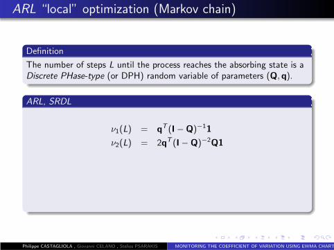
Definition
The number of steps L until the process reaches the absorbing state is aDiscrete PHase-type (or DPH) random variable of parameters (Q,q).
Philippe CASTAGLIOLA , Giovanni CELANO , Stelios PSARAKIS MONITORING THE COEFFICIENT OF VARIATION USING EWMA CHARTS

ARL “local” optimization (Markov chain)
Definition
The number of steps L until the process reaches the absorbing state is aDiscrete PHase-type (or DPH) random variable of parameters (Q,q).
ARL, SRDL
ν1(L) = qT (I − Q)−11
Philippe CASTAGLIOLA , Giovanni CELANO , Stelios PSARAKIS MONITORING THE COEFFICIENT OF VARIATION USING EWMA CHARTS
ARL “local” optimization (Markov chain)
Definition
The number of steps L until the process reaches the absorbing state is aDiscrete PHase-type (or DPH) random variable of parameters (Q,q).
ARL, SRDL
ν1(L) = qT (I − Q)−11
ν2(L) = 2qT (I − Q)−2Q1
Philippe CASTAGLIOLA , Giovanni CELANO , Stelios PSARAKIS MONITORING THE COEFFICIENT OF VARIATION USING EWMA CHARTS

ARL “local” optimization (Markov chain)
Definition
The number of steps L until the process reaches the absorbing state is aDiscrete PHase-type (or DPH) random variable of parameters (Q,q).
ARL, SRDL
ν1(L) = qT (I − Q)−11
ν2(L) = 2qT (I − Q)−2Q1
and
ARL = ν1(L)
SDRL =√
ν2(L) − ν21(L) + ν1(L)
Philippe CASTAGLIOLA , Giovanni CELANO , Stelios PSARAKIS MONITORING THE COEFFICIENT OF VARIATION USING EWMA CHARTS

Optimal (λ∗, K ∗) and ARL for EWMA-γ2 and SH-γ charts
n = 7, ARL0 = 370.4τ γ0 = 0.05 γ0 = 0.1 γ0 = 0.15 γ0 = 0.2
0.50 (0.5671, 1.8734) (0.5637, 1.8480) (0.5608, 1.8043) (0.5539, 1.7474)(3.4, 18.4) (3.4, 18.6) (3.5, 18.9) (3.5, 19.3)
0.65 (0.2951, 2.1229) (0.2902, 2.0932) (0.2854, 2.0416) (0.2792, 1.9709)(6.4, 69.3) (6.4, 69.9) (6.4, 70.8) (6.5, 72.1)
0.80 (0.1104, 2.2582) (0.1088, 2.2142) (0.1032, 2.1413) (0.0976, 2.0414)(15.3, 212.1) (15.4, 213.2) (15.5, 215.0) (15.6, 217.5)
1.25 (0.1092, 3.0381) (0.1101, 3.0831) (0.1097, 3.1504) (0.1087, 3.2443)(11.3, 32.4) (11.4, 32.9) (11.7, 33.8) (12.0, 35.1)
1.50 (0.2646, 3.5219) (0.2603, 3.5538) (0.2531, 3.6078) (0.2443, 3.6873)(4.3, 7.2) (4.3, 7.4) (4.4, 7.6) (4.6, 8.0)
2.00 (0.5852, 3.9768) (0.5725, 4.0146) (0.5520, 4.0781) (0.5212, 4.1644)(1.8, 2.1) (1.8, 2.1) (1.9, 2.2) (2.0, 2.3)
Philippe CASTAGLIOLA , Giovanni CELANO , Stelios PSARAKIS MONITORING THE COEFFICIENT OF VARIATION USING EWMA CHARTS

(λ∗, K ∗) nomograms
0
0.1
0.2
0.3
0.4
0.5
0.6
0.7
0.8
0.9
1
0.6 0.8 1 1.2 1.4 1.6 1.8 2
n=5n=7
n=10n=15
λ
τ
γ0 = 0.05
λ−∗ λ+∗
1.5
2
2.5
3
3.5
4
4.5
0.6 0.8 1 1.2 1.4 1.6 1.8 2
n=5n=7
n=10n=15
K
τ
γ0 = 0.05
K−∗ K+∗
0
0.1
0.2
0.3
0.4
0.5
0.6
0.7
0.8
0.9
1
0.6 0.8 1 1.2 1.4 1.6 1.8 2
n=5n=7
n=10n=15
λ
τ
λ−∗ λ+∗
γ0 = 0.1
1.5
2
2.5
3
3.5
4
4.5
0.6 0.8 1 1.2 1.4 1.6 1.8 2
n=5n=7
n=10n=15
K
τ
K−∗ K+∗
γ0 = 0.1
Philippe CASTAGLIOLA , Giovanni CELANO , Stelios PSARAKIS MONITORING THE COEFFICIENT OF VARIATION USING EWMA CHARTS

(λ∗, K ∗) nomograms
0
0.1
0.2
0.3
0.4
0.5
0.6
0.7
0.8
0.9
1
0.6 0.8 1 1.2 1.4 1.6 1.8 2
n=5n=7
n=10n=15
λ
τ
γ0 = 0.15
λ−∗ λ+∗
1.5
2
2.5
3
3.5
4
4.5
0.6 0.8 1 1.2 1.4 1.6 1.8 2
n=5n=7
n=10n=15
K
τ
γ0 = 0.15
K−∗ K+∗
0
0.1
0.2
0.3
0.4
0.5
0.6
0.7
0.8
0.9
1
0.6 0.8 1 1.2 1.4 1.6 1.8 2
n=5n=7
n=10n=15
λ
τ
λ−∗ λ+∗
γ0 = 0.2
1.5
2
2.5
3
3.5
4
4.5
0.6 0.8 1 1.2 1.4 1.6 1.8 2
n=5n=7
n=10n=15
K
τ
K−∗ K+∗
γ0 = 0.2
Philippe CASTAGLIOLA , Giovanni CELANO , Stelios PSARAKIS MONITORING THE COEFFICIENT OF VARIATION USING EWMA CHARTS

EWMA-γ2 chart v.s. EWMA-γ (Hong et al., 2008) chart
n = 5τ γ0 = 0.05 γ0 = 0.1 γ0 = 0.15 γ0 = 0.2
0.50 (4.8, 4.7) (4.8, 4.7) (4.8, 4.8) (4.8, 4.8)0.65 (8.7, 8.8) (8.8, 8.9) (8.8, 8.9) (8.8, 9.0)0.80 (20.6, 21.1) (20.6, 21.2) (20.7, 21.3) (20.9, 21.5)0.90 (53.2, 56.2) (53.7, 56.4) (54.5, 56.8) (55.8, 57.3)1.10 (51.0, 51.5) (51.2, 51.8) (51.7, 52.3) (52.4, 52.9)1.25 (15.0, 15.5) (15.2, 15.6) (15.4, 15.8) (15.9, 16.0)1.50 (5.7, 5.9) (5.8, 5.9) (5.9, 6.0) (6.1, 6.2)2.00 (2.4, 2.4) (2.4, 2.4) (2.5, 2.5) (2.6, 2.6)
n = 7τ γ0 = 0.05 γ0 = 0.1 γ0 = 0.15 γ0 = 0.2
0.50 (3.4, 3.4) (3.4, 3.4) (3.5, 3.4) (3.5, 3.5)0.65 (6.4, 6.4) (6.4, 6.4) (6.4, 6.5) (6.5, 6.5)0.80 (15.3, 15.6) (15.4, 15.6) (15.5, 15.8) (15.6, 16.0)0.90 (40.4, 41.8) (40.7, 42.0) (41.2, 42.4) (42.0, 42.9)1.10 (39.2, 39.7) (39.5, 40.0) (40.1, 40.4) (40.9, 41.1)1.25 (11.3, 11.5) (11.4, 11.6) (11.7, 11.8) (12.0, 12.1)1.50 (4.3, 4.3) (4.3, 4.4) (4.4, 4.5) (4.6, 4.6)2.00 (1.8, 1.8) (1.8, 1.8) (1.9, 1.9) (2.0, 2.0)
Philippe CASTAGLIOLA , Giovanni CELANO , Stelios PSARAKIS MONITORING THE COEFFICIENT OF VARIATION USING EWMA CHARTS
ARL “global” optimization
Philippe CASTAGLIOLA , Giovanni CELANO , Stelios PSARAKIS MONITORING THE COEFFICIENT OF VARIATION USING EWMA CHARTS

ARL “global” optimization
Drawback of “local” optimization
Philippe CASTAGLIOLA , Giovanni CELANO , Stelios PSARAKIS MONITORING THE COEFFICIENT OF VARIATION USING EWMA CHARTS

ARL “global” optimization
Drawback of “local” optimization
Usually the quality practitioner does not know in advance the entityof the next shift size because of the lack of related historical data.
The shift size is not deterministic and varies accordingly to someunknown stochastic model.
New objective function and constraint
Find out the optimal couples (λ∗,K∗) such that :
(λ∗,K∗) = argmin(λ,K)
EARL(γ0, τγ0, λ,K , n)
withEARL =
∫
fτ (τ)ARL(γ0, τγ0, λ,K , n)dτ.
subject to the constraint
EARL(γ0, γ0, λ,K , n) = ARL(γ0, γ0, λ,K , n) = ARL0,
fτ (τ) is the p.d.f. of the shift τ
Philippe CASTAGLIOLA , Giovanni CELANO , Stelios PSARAKIS MONITORING THE COEFFICIENT OF VARIATION USING EWMA CHARTS

ARL “global” optimization
Drawback of “local” optimization
Usually the quality practitioner does not know in advance the entityof the next shift size because of the lack of related historical data.
The shift size is not deterministic and varies accordingly to someunknown stochastic model.
New objective function and constraint
Find out the optimal couples (λ∗,K∗) such that :
(λ∗,K∗) = argmin(λ,K)
EARL(γ0, τγ0, λ,K , n)
withEARL =
∫
fτ (τ)ARL(γ0, τγ0, λ,K , n)dτ.
subject to the constraint
EARL(γ0, γ0, λ,K , n) = ARL(γ0, γ0, λ,K , n) = ARL0,
fτ (τ) is the p.d.f. of the shift τ → uniform distribution over [0.5, 1)(decreasing case)
Philippe CASTAGLIOLA , Giovanni CELANO , Stelios PSARAKIS MONITORING THE COEFFICIENT OF VARIATION USING EWMA CHARTS

ARL “global” optimization
Drawback of “local” optimization
Usually the quality practitioner does not know in advance the entityof the next shift size because of the lack of related historical data.
The shift size is not deterministic and varies accordingly to someunknown stochastic model.
New objective function and constraint
Find out the optimal couples (λ∗,K∗) such that :
(λ∗,K∗) = argmin(λ,K)
EARL(γ0, τγ0, λ,K , n)
withEARL =
∫
fτ (τ)ARL(γ0, τγ0, λ,K , n)dτ.
subject to the constraint
EARL(γ0, γ0, λ,K , n) = ARL(γ0, γ0, λ,K , n) = ARL0,
fτ (τ) is the p.d.f. of the shift τ → uniform distribution over [0.5, 1)(decreasing case) and over (1, 2] (increasing case).
Philippe CASTAGLIOLA , Giovanni CELANO , Stelios PSARAKIS MONITORING THE COEFFICIENT OF VARIATION USING EWMA CHARTS

ARL “global” optimization
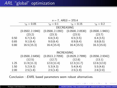
n = 7, ARL0 = 370.4γ0 = 0.05 γ0 = 0.1 γ0 = 0.15 γ0 = 0.2
DECREASING(0.0502, 2.1940) (0.0500, 2.1392) (0.0500, 2.0530) (0.0500, 1.9401)
(23.2) (23.3) (23.5) (23.7)0.50 6.7 (3.4) 6.6 (3.4) 6.5 (3.5) 6.4 (3.5)0.65 9.1 (6.4) 9.0 (6.4) 8.9 (6.4) 8.8 (6.5)0.80 16.5 (15.3) 16.4 (15.4) 16.4 (15.5) 16.3 (15.6)
INCREASING(0.0500, 2.6456) (0.0513, 2.7059) (0.0529, 2.7999) (0.0556, 2.9342)
(12.5) (12.7) (12.8) (13.1)1.25 11.9 (11.3) 12.0 (11.4) 12.3 (11.7) 12.6 (12.0)1.50 5.2 (4.3) 5.3 (4.3) 5.4 (4.4) 5.5 (4.6)2.00 2.5 (1.8) 2.5 (1.8) 2.5 (1.9) 2.6 (2.0)
Philippe CASTAGLIOLA , Giovanni CELANO , Stelios PSARAKIS MONITORING THE COEFFICIENT OF VARIATION USING EWMA CHARTS

ARL “global” optimization
n = 7, ARL0 = 370.4γ0 = 0.05 γ0 = 0.1 γ0 = 0.15 γ0 = 0.2
DECREASING(0.0502, 2.1940) (0.0500, 2.1392) (0.0500, 2.0530) (0.0500, 1.9401)
(23.2) (23.3) (23.5) (23.7)0.50 6.7 (3.4) 6.6 (3.4) 6.5 (3.5) 6.4 (3.5)0.65 9.1 (6.4) 9.0 (6.4) 8.9 (6.4) 8.8 (6.5)0.80 16.5 (15.3) 16.4 (15.4) 16.4 (15.5) 16.3 (15.6)
INCREASING(0.0500, 2.6456) (0.0513, 2.7059) (0.0529, 2.7999) (0.0556, 2.9342)
(12.5) (12.7) (12.8) (13.1)1.25 11.9 (11.3) 12.0 (11.4) 12.3 (11.7) 12.6 (12.0)1.50 5.2 (4.3) 5.3 (4.3) 5.4 (4.4) 5.5 (4.6)2.00 2.5 (1.8) 2.5 (1.8) 2.5 (1.9) 2.6 (2.0)
Philippe CASTAGLIOLA , Giovanni CELANO , Stelios PSARAKIS MONITORING THE COEFFICIENT OF VARIATION USING EWMA CHARTS
ARL “global” optimization
n = 7, ARL0 = 370.4γ0 = 0.05 γ0 = 0.1 γ0 = 0.15 γ0 = 0.2
DECREASING(0.0502, 2.1940) (0.0500, 2.1392) (0.0500, 2.0530) (0.0500, 1.9401)
(23.2) (23.3) (23.5) (23.7)0.50 6.7 (3.4) 6.6 (3.4) 6.5 (3.5) 6.4 (3.5)0.65 9.1 (6.4) 9.0 (6.4) 8.9 (6.4) 8.8 (6.5)0.80 16.5 (15.3) 16.4 (15.4) 16.4 (15.5) 16.3 (15.6)
INCREASING(0.0500, 2.6456) (0.0513, 2.7059) (0.0529, 2.7999) (0.0556, 2.9342)
(12.5) (12.7) (12.8) (13.1)1.25 11.9 (11.3) 12.0 (11.4) 12.3 (11.7) 12.6 (12.0)1.50 5.2 (4.3) 5.3 (4.3) 5.4 (4.4) 5.5 (4.6)2.00 2.5 (1.8) 2.5 (1.8) 2.5 (1.9) 2.6 (2.0)
Conclusion : EARL based parameters seem robust alternatives.
Philippe CASTAGLIOLA , Giovanni CELANO , Stelios PSARAKIS MONITORING THE COEFFICIENT OF VARIATION USING EWMA CHARTS

An illustrative example
Philippe CASTAGLIOLA , Giovanni CELANO , Stelios PSARAKIS MONITORING THE COEFFICIENT OF VARIATION USING EWMA CHARTS

An illustrative example
A sintering (frittage) process manufacturing mechanical parts
Philippe CASTAGLIOLA , Giovanni CELANO , Stelios PSARAKIS MONITORING THE COEFFICIENT OF VARIATION USING EWMA CHARTS

An illustrative example
A sintering (frittage) process manufacturing mechanical parts
Produced parts are required to guarantee a pressure test drop timeTpd from 2 bar to 1.5 bar larger than 30 sec.
A Regression study demonstrated the presence of a constantproportionality σpd = γpd × µpd between the standard deviation ofthe pressure drop time and its mean.
Philippe CASTAGLIOLA , Giovanni CELANO , Stelios PSARAKIS MONITORING THE COEFFICIENT OF VARIATION USING EWMA CHARTS

An illustrative example
A sintering (frittage) process manufacturing mechanical parts
Produced parts are required to guarantee a pressure test drop timeTpd from 2 bar to 1.5 bar larger than 30 sec.
A Regression study demonstrated the presence of a constantproportionality σpd = γpd × µpd between the standard deviation ofthe pressure drop time and its mean.⇒ the coefficient of variation γpd will be monitored.
Phase I dataset
m = 20 sample data, each having sample size n = 5.
Estimation of the nominal coefficient of variation γ0 = 0.417.
Control limits of the SH-γ chart
LCLSH = F−1γ
(
0.00272 |5, 0.417
)
= 0.064725,
UCLSH = F−1γ
(
1 − 0.00272 |5, 0.417
)
= 1.216527.
Philippe CASTAGLIOLA , Giovanni CELANO , Stelios PSARAKIS MONITORING THE COEFFICIENT OF VARIATION USING EWMA CHARTS

An illustrative example (SH-γ chart, Phase I)
0
0.2
0.4
0.6
0.8
1
1.2
1.4
0 5 10 15 20
Sample Number
LCL=0.0647
UCL=1.2165
γ0 = 0.417
γk
SH-γ chart
Philippe CASTAGLIOLA , Giovanni CELANO , Stelios PSARAKIS MONITORING THE COEFFICIENT OF VARIATION USING EWMA CHARTS

An illustrative example (SH-γ chart, Phase I)
0
0.2
0.4
0.6
0.8
1
1.2
1.4
0 5 10 15 20
Sample Number
LCL=0.0647
UCL=1.2165
γ0 = 0.417
γk
SH-γ chart, The sintering process seems in-control.
Philippe CASTAGLIOLA , Giovanni CELANO , Stelios PSARAKIS MONITORING THE COEFFICIENT OF VARIATION USING EWMA CHARTS

An illustrative example (EWMA-γ2 chart)
Philippe CASTAGLIOLA , Giovanni CELANO , Stelios PSARAKIS MONITORING THE COEFFICIENT OF VARIATION USING EWMA CHARTS

An illustrative example (EWMA-γ2 chart)
Optimal parameters
Philippe CASTAGLIOLA , Giovanni CELANO , Stelios PSARAKIS MONITORING THE COEFFICIENT OF VARIATION USING EWMA CHARTS

An illustrative example (EWMA-γ2 chart)
Optimal parameters
Accordingly to the process engineer experience, an increase of 25%in the coefficient of variation should be interpreted as a signal thatsomething is going wrong.
Philippe CASTAGLIOLA , Giovanni CELANO , Stelios PSARAKIS MONITORING THE COEFFICIENT OF VARIATION USING EWMA CHARTS

An illustrative example (EWMA-γ2 chart)
Optimal parameters
Accordingly to the process engineer experience, an increase of 25%in the coefficient of variation should be interpreted as a signal thatsomething is going wrong.⇒ τ = 1.25.
Optimizing algorithm yields λ+∗ = 0.0793 and K+∗ = 4.3699.
Upper Control Limit of the EWMA-γ2 chart
Approximations yield µ0(γ2) = 0.1557 and σ0(γ
2) = 0.1643.
UCLEWMA−γ2 = 0.1557 + 4.3699 ×√
0.0793
2 − 0.0793× 0.1643 = 0.3016.
Philippe CASTAGLIOLA , Giovanni CELANO , Stelios PSARAKIS MONITORING THE COEFFICIENT OF VARIATION USING EWMA CHARTS

An illustrative example (EWMA-γ chart, Phase I)
0
0.05
0.1
0.15
0.2
0.25
0.3
0.35
0.4
0 5 10 15 20
Sample Number
UCL=0.3016
γ2 k
EWMA-γ2 chart
Philippe CASTAGLIOLA , Giovanni CELANO , Stelios PSARAKIS MONITORING THE COEFFICIENT OF VARIATION USING EWMA CHARTS

An illustrative example (EWMA-γ chart, Phase I)
0
0.05
0.1
0.15
0.2
0.25
0.3
0.35
0.4
0 5 10 15 20
Sample Number
UCL=0.3016
γ2 k
EWMA-γ2 chart, The sintering process seems in-control too.
Philippe CASTAGLIOLA , Giovanni CELANO , Stelios PSARAKIS MONITORING THE COEFFICIENT OF VARIATION USING EWMA CHARTS

An illustrative example (SH-γ chart, Phase II)
Philippe CASTAGLIOLA , Giovanni CELANO , Stelios PSARAKIS MONITORING THE COEFFICIENT OF VARIATION USING EWMA CHARTS
An illustrative example (SH-γ chart, Phase II)
Phase II : 20 new samples of size n = 5 taken from the process after theoccurrence of a special cause increasing process variability.
Philippe CASTAGLIOLA , Giovanni CELANO , Stelios PSARAKIS MONITORING THE COEFFICIENT OF VARIATION USING EWMA CHARTS

An illustrative example (SH-γ chart, Phase II)
Phase II : 20 new samples of size n = 5 taken from the process after theoccurrence of a special cause increasing process variability.
0
0.2
0.4
0.6
0.8
1
1.2
1.4
0 5 10 15 20
Sample Number
LCL=0.0647
UCL=1.2165
γ0 = 0.417
γk
SH-γ chart
Philippe CASTAGLIOLA , Giovanni CELANO , Stelios PSARAKIS MONITORING THE COEFFICIENT OF VARIATION USING EWMA CHARTS

An illustrative example (SH-γ chart, Phase II)
Phase II : 20 new samples of size n = 5 taken from the process after theoccurrence of a special cause increasing process variability.
0
0.2
0.4
0.6
0.8
1
1.2
1.4
0 5 10 15 20
Sample Number
LCL=0.0647
UCL=1.2165
γ0 = 0.417
γk
SH-γ chart, The sintering process seems in-control...
Philippe CASTAGLIOLA , Giovanni CELANO , Stelios PSARAKIS MONITORING THE COEFFICIENT OF VARIATION USING EWMA CHARTS

An illustrative example (EWMA-γ2 chart, Phase II)
0
0.05
0.1
0.15
0.2
0.25
0.3
0.35
0.4
0 5 10 15 20
Sample Number
UCL=0.3016
γ2 k
EWMA-γ2 chart
Philippe CASTAGLIOLA , Giovanni CELANO , Stelios PSARAKIS MONITORING THE COEFFICIENT OF VARIATION USING EWMA CHARTS

An illustrative example (EWMA-γ2 chart, Phase II)
0
0.05
0.1
0.15
0.2
0.25
0.3
0.35
0.4
0 5 10 15 20
Sample Number
UCL=0.3016
γ2 k
EWMA-γ2 chart, ... but in fact it is not !
Philippe CASTAGLIOLA , Giovanni CELANO , Stelios PSARAKIS MONITORING THE COEFFICIENT OF VARIATION USING EWMA CHARTS

An illustrative example (Xk , Phase II)
200
400
600
800
1000
1200
1400
1600
0 5 10 15 20
Sample Number
823.55
X
Xk
Philippe CASTAGLIOLA , Giovanni CELANO , Stelios PSARAKIS MONITORING THE COEFFICIENT OF VARIATION USING EWMA CHARTS

An illustrative example (Sk , Phase II)
0
200
400
600
800
1000
1200
1400
1600
1800
0 5 10 15 20
Sample Number
331.5
Abnormal pattern
S
Sk
Philippe CASTAGLIOLA , Giovanni CELANO , Stelios PSARAKIS MONITORING THE COEFFICIENT OF VARIATION USING EWMA CHARTS

Conclusions
Philippe CASTAGLIOLA , Giovanni CELANO , Stelios PSARAKIS MONITORING THE COEFFICIENT OF VARIATION USING EWMA CHARTS

Conclusions
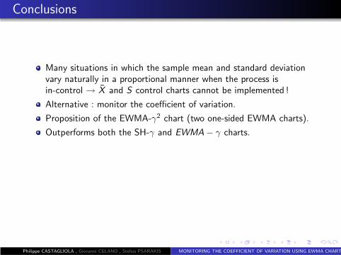
Many situations in which the sample mean and standard deviationvary naturally in a proportional manner when the process isin-control
Philippe CASTAGLIOLA , Giovanni CELANO , Stelios PSARAKIS MONITORING THE COEFFICIENT OF VARIATION USING EWMA CHARTS

Conclusions
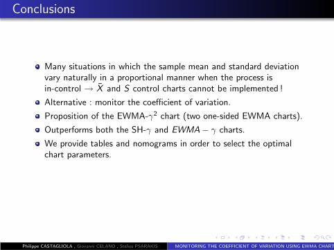
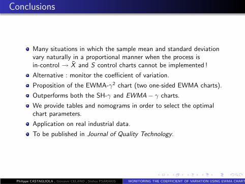
Many situations in which the sample mean and standard deviationvary naturally in a proportional manner when the process isin-control → X and S control charts cannot be implemented !
Philippe CASTAGLIOLA , Giovanni CELANO , Stelios PSARAKIS MONITORING THE COEFFICIENT OF VARIATION USING EWMA CHARTS

Conclusions
Many situations in which the sample mean and standard deviationvary naturally in a proportional manner when the process isin-control → X and S control charts cannot be implemented !
Alternative : monitor the coefficient of variation.
Proposition of the EWMA-γ2 chart (two one-sided EWMA charts).
Philippe CASTAGLIOLA , Giovanni CELANO , Stelios PSARAKIS MONITORING THE COEFFICIENT OF VARIATION USING EWMA CHARTS
Conclusions
Many situations in which the sample mean and standard deviationvary naturally in a proportional manner when the process isin-control → X and S control charts cannot be implemented !
Alternative : monitor the coefficient of variation.
Proposition of the EWMA-γ2 chart (two one-sided EWMA charts).
Outperforms both the SH-γ and EWMA − γ charts.
We provide tables and nomograms in order to select the optimalchart parameters.
Application on real industrial data.
To be published in Journal of Quality Technology.
Philippe CASTAGLIOLA , Giovanni CELANO , Stelios PSARAKIS MONITORING THE COEFFICIENT OF VARIATION USING EWMA CHARTS

![f B i a l os u r o n tatits Journal of Biometrics ... · deviation or coefficient of variation (CV) under the specified conditions of measurement [3]. Then, coefficient of variation](https://img.pdfslide.us/doc/110x75/5fb3ea1e70df8352ab3f8dd6/f-b-i-a-l-os-u-r-o-n-tatits-journal-of-biometrics-deviation-or-coefficient-of.jpg)


![Untitled-1 [gencap.org.in] · rainfall of 568.5 mm with a coefficient of variation (C V) of 28 cent. That the coefficient of variation of rainfall is higher than the threshold level](https://img.pdfslide.us/doc/110x75/60318d4b82f0fc5aab284f08/untitled-1-rainfall-of-5685-mm-with-a-coefficient-of-variation-c-v-of-28.jpg)


![· Median Mode Variance 58.4 - 56.8 54.2 = 21.16 Calculate the Pearson's Coefficient of Variation 2 Kira Pearson 's Coefficient of Variation 2 [4 marks] [4 markah] Determine the](https://img.pdfslide.us/doc/110x75/5e2a8b84b2b85f284b45c89f/median-mode-variance-584-568-542-2116-calculate-the-pearsons-coefficient.jpg)