Monitoring milk-powder dryers via Bayesian

inference in an FPGA

Colin Fox fox@physics.otago.ac.nz

Markus Neumayer, Al Parker, Pat Suggate

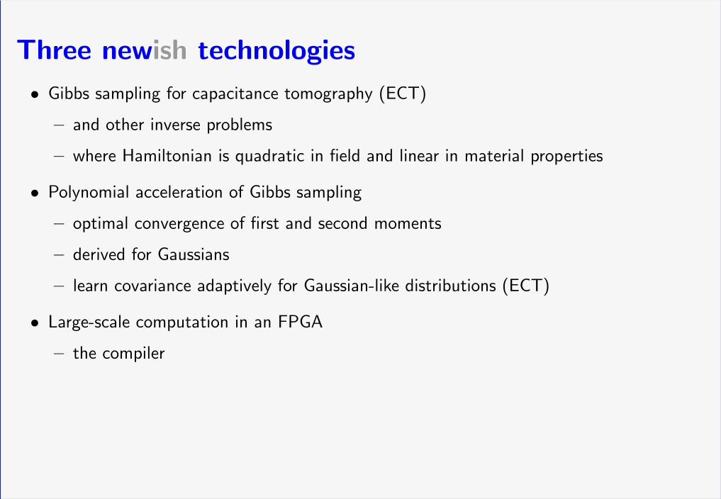
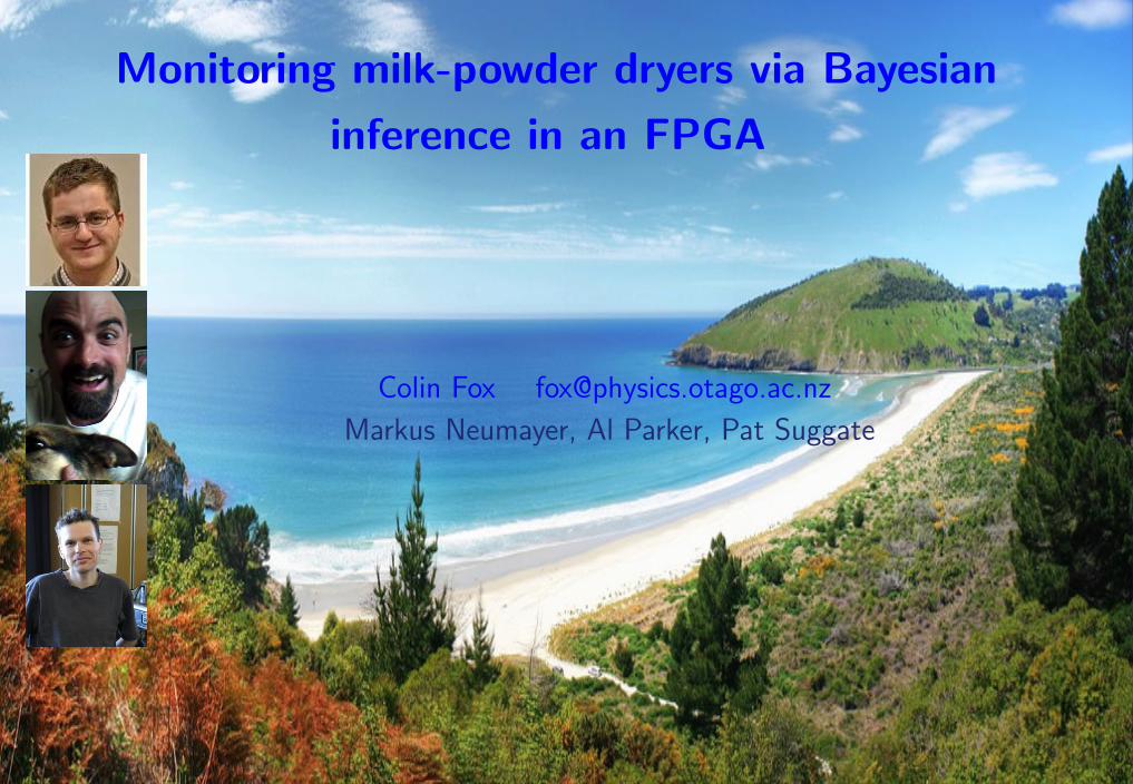
Three newish technologies

• Gibbs sampling for capacitance tomography (ECT)

– and other inverse problems

– where Hamiltonian is quadratic in field and linear in material properties

• Polynomial acceleration of Gibbs sampling

– optimal convergence of first and second moments

– derived for Gaussians

– learn covariance adaptively for Gaussian-like distributions (ECT)

• Large-scale computation in an FPGA

– the compiler

Two Paradigms for Imaging

• Signal processing

– solution is function of data

• Model fitting

– optimization (best solution)

– statistical inference (summarize all solutions)

Bayesian inference is the ‘gold standard’ though intensive in computing and modelling

We currently implement Bayesian inference for:

• Wildlife tracking

• Dairy processing

• Agritech

• Geothermal electricity generation

Two Paradigms for Imaging

• Signal processing

– solution is function of data

• Model fitting

– optimization (best solution)

– statistical inference (summarize all solutions)

Bayesian inference is the ‘gold standard’ though intensive in computing and modelling

We currently implement statistical inference for:

• Wildlife tracking (DoC, Sirtrack, Rakon)

• Dairy processing (TetraPak, Synlait)

• Agritech (Truetest, Silverfern Farms)

• Geothermal electricity generation (Contact Energy, iwi)

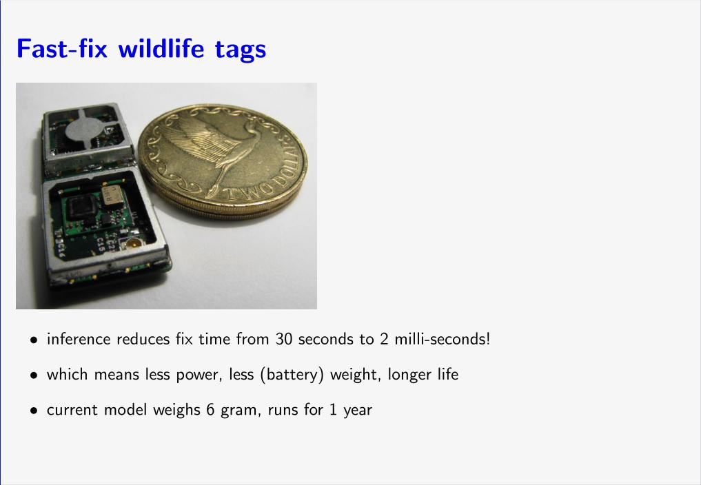
Fast-fix wildlife tags

• inference reduces fix time from 30 seconds to 2 milli-seconds!

• which means less power, less (battery) weight, longer life

• current model weighs 6 gram, runs for 1 year

Royal Albatross at Tiaroa Head

http://www.physics.otago.ac.nz/tags/

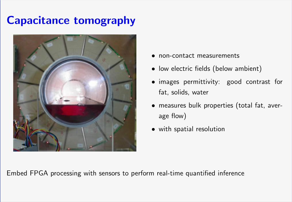
Capacitance tomography

• non-contact measurements

• low electric fields (below ambient)

• images permittivity: good contrast for

fat, solids, water

• measures bulk properties (total fat, aver-

age flow)

• with spatial resolution

Embed FPGA processing with sensors to perform real-time quantified inference

Edendale plant

Burt Munro

Sample-based Bayesian inference

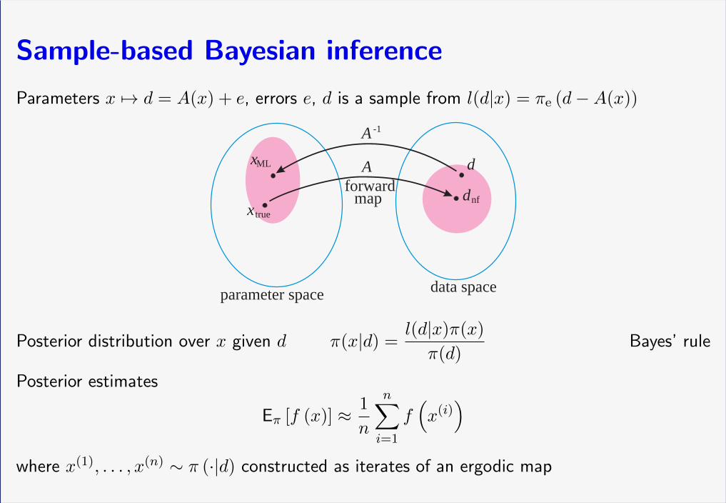
Parameters x 7→ d = A(x) + e, errors e, d is a sample from l(d|x) = πe (d−A(x))

parameter space data space

x true

xML d

dnfforward

map

A

A -1

Posterior distribution over x given d π(x|d) =l(d|x)π(x)

π(d)Bayes’ rule

Posterior estimates

Eπ [f (x)] ≈ 1

n

n∑i=1

f(x(i))

where x(1), . . . , x(n) ∼ π (·|d) constructed as iterates of an ergodic map

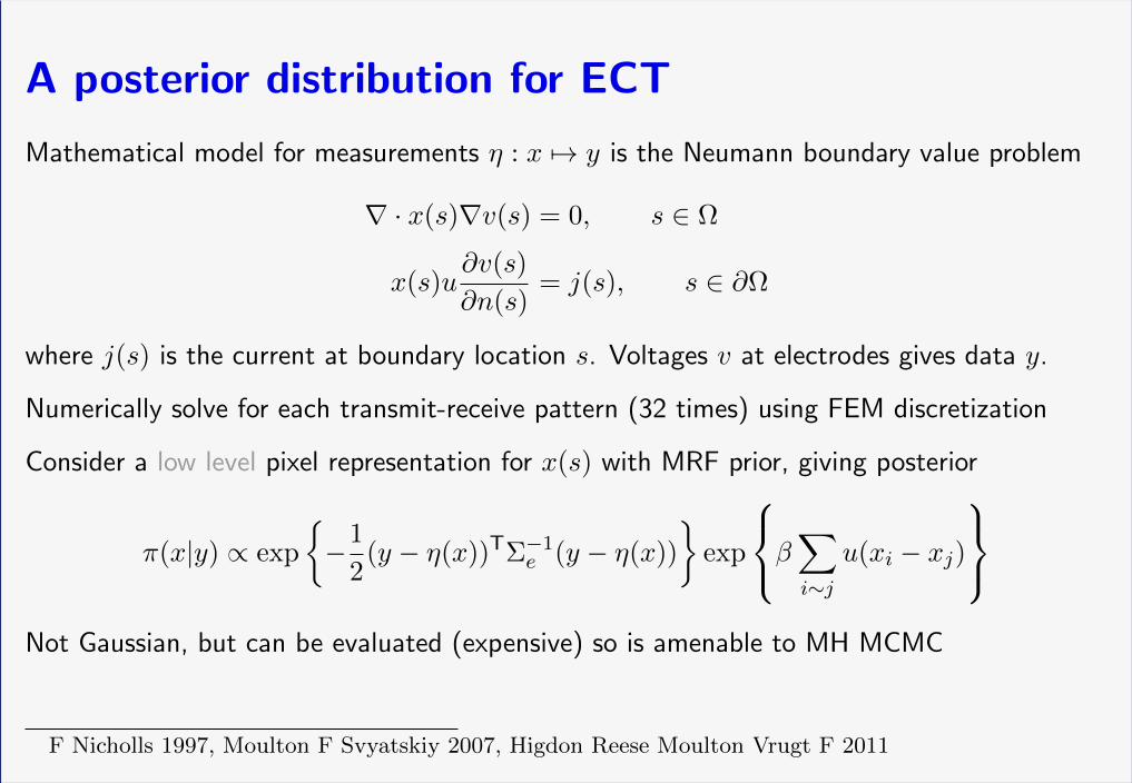
A posterior distribution for ECT

Mathematical model for measurements η : x 7→ y is the Neumann boundary value problem

∇ · x(s)∇v(s) = 0, s ∈ Ω

x(s)u∂v(s)

∂n(s)= j(s), s ∈ ∂Ω

where j(s) is the current at boundary location s. Voltages v at electrodes gives data y.

Numerically solve for each transmit-receive pattern (32 times) using FEM discretization

Consider a low level pixel representation for x(s) with MRF prior, giving posterior

π(x|y) ∝ exp

−1

2(y − η(x))TΣ−1

e (y − η(x))

exp

β∑i∼j

u(xi − xj)

Not Gaussian, but can be evaluated (expensive) so is amenable to MH MCMC

F Nicholls 1997, Moulton F Svyatskiy 2007, Higdon Reese Moulton Vrugt F 2011

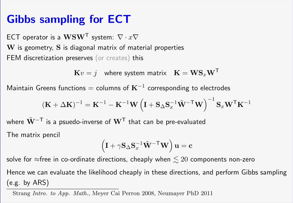
Gibbs sampling for ECT

ECT operator is a WSWT system: ∇ · x∇W is geometry, S is diagonal matrix of material properties

FEM discretization preserves (or creates) this

Kv = j where system matrix K = WSxWT

Maintain Greens functions = columns of K−1 corresponding to electrodes

(K + ∆K)−1 = K−1 −K−1W(I + S∆S−1

x W−TW)−1

SxWTK−1

where W−T is a psuedo-inverse of WT that can be pre-evaluated

The matrix pencil (I + γS∆S−1

x W−TW)u = c

solve for ≈free in co-ordinate directions, cheaply when . 20 components non-zero

Hence we can evaluate the likelihood cheaply in these directions, and perform Gibbs sampling

(e.g. by ARS)

Strang Intro. to App. Math., Meyer Cai Perron 2008, Neumayer PhD 2011

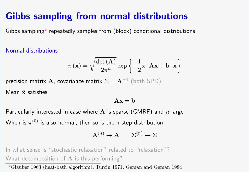
Gibbs sampling from normal distributions

Gibbs samplinga repeatedly samples from (block) conditional distributions

Normal distributions

π (x) =

√det (A)

2πnexp

−1

2xTAx + bTx

precision matrix A, covariance matrix Σ = A−1 (both SPD)

Mean x satisfies

Ax = b

Particularly interested in case where A is sparse (GMRF) and n large

When is π(0) is also normal, then so is the n-step distribution

A(n) → A Σ(n) → Σ

In what sense is “stochastic relaxation” related to “relaxation”?

What decomposition of A is this performing?aGlauber 1963 (heat-bath algorithm), Turcin 1971, Geman and Geman 1984

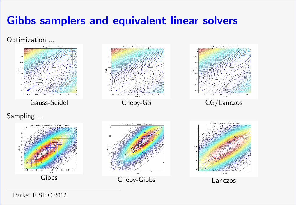
Gibbs samplers and equivalent linear solvers

Optimization ...

Gauss-Seidel Cheby-GS CG/Lanczos

Sampling ...

Gibbs Cheby-Gibbs Lanczos

Parker F SISC 2012

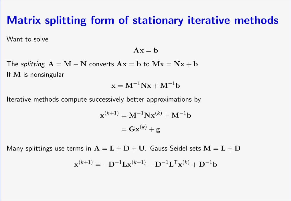
Matrix splitting form of stationary iterative methods

Want to solve

Ax = b

The splitting A = M−N converts Ax = b to Mx = Nx + b

If M is nonsingular

x = M−1Nx + M−1b

Iterative methods compute successively better approximations by

x(k+1) = M−1Nx(k) + M−1b

= Gx(k) + g

Many splittings use terms in A = L + D + U. Gauss-Seidel sets M = L + D

x(k+1) = −D−1Lx(k+1) −D−1LTx(k) + D−1b

Matrix formulation of Gibbs sampling from N(0,A−1)

Let y = (y1, y2, ..., yn)T

Component-wise Gibbs updates each component in sequence from the (normal) conditional

distributions

One ‘sweep’ over all n components can be written

y(k+1) = −D−1Ly(k+1) −D−1LTy(k) + D−1/2z(k)

where: D = diag(A), L is the strictly lower triangular part of A, z(k−1) ∼ N(0, I)

y(k+1) = Gy(k) + c(k)

c(k) is iid ’noise’ with zero mean, finite covariance

Spot the similarity to Gauss-Seidel iteration for solving Ax = b

x(k+1) = −D−1Lx(k+1) −D−1LTx(k) + D−1b

Goodman & Sokal 1989; Amit & Grenander 1991

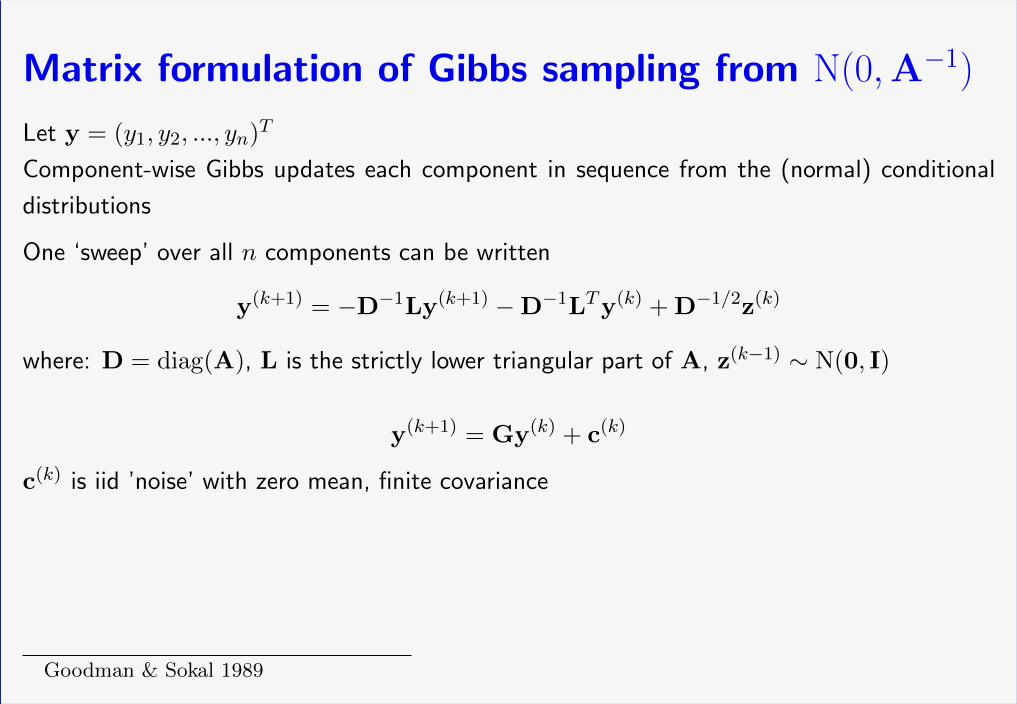
Matrix formulation of Gibbs sampling from N(0,A−1)

Let y = (y1, y2, ..., yn)T

Component-wise Gibbs updates each component in sequence from the (normal) conditional

distributions

One ‘sweep’ over all n components can be written

y(k+1) = −D−1Ly(k+1) −D−1LTy(k) + D−1/2z(k)

where: D = diag(A), L is the strictly lower triangular part of A, z(k−1) ∼ N(0, I)

y(k+1) = Gy(k) + c(k)

c(k) is iid ’noise’ with zero mean, finite covariance

Spot the similarity to Gauss-Seidel iteration for solving Ax = b

x(k+1) = −D−1Lx(k+1) −D−1LTx(k) + D−1b

Goodman & Sokal 1989; Amit & Grenander 1991

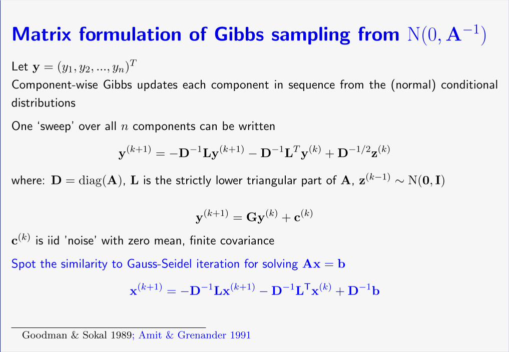
Gibbs converges ⇐⇒ solver converges

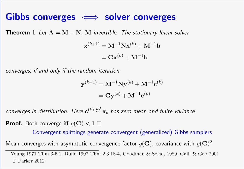
Theorem 1 Let A = M−N, M invertible. The stationary linear solver

x(k+1) = M−1Nx(k) + M−1b

= Gx(k) + M−1b

converges, if and only if the random iteration

y(k+1) = M−1Ny(k) + M−1c(k)

= Gy(k) + M−1c(k)

converges in distribution. Here c(k) iid∼ πn has zero mean and finite variance

Proof. Both converge iff %(G) < 1

Convergent splittings generate convergent (generalized) Gibbs samplers

Mean converges with asymptotic convergence factor %(G), covariance with %(G)2

Young 1971 Thm 3-5.1, Duflo 1997 Thm 2.3.18-4, Goodman & Sokal, 1989, Galli & Gao 2001

F Parker 2012

Some not so common Gibbs samplers for N(0,A−1)

splitting/sampler M Var(c(k)

)= MT + N converge if

Richardson 1ω I

2ω I−A 0 < ω <

2

%(A)

Jacobi D 2D−A A SDD

GS/Gibbs D + L D always

SOR/B&F 1ωD + L 2−ω

ω D 0 < ω < 2

SSOR/REGS ω2−ωMSORD

−1MTSOR

ω2−ω

(MSORD

−1MTSOR 0 < ω < 2

+NTSORD

−1NSOR

)Good choice has: convenient to solve Mu = r and sample from N(0,MT + N)

Relaxation parameter ω can accelerate Gibbs

SSOR is a forwards and backwards sweep of SOR to give a symmetric splitting

SOR: Adler 1981; Barone & Frigessi 1990, Amit & Grenander 1991, SSOR: Roberts & Sahu 1997

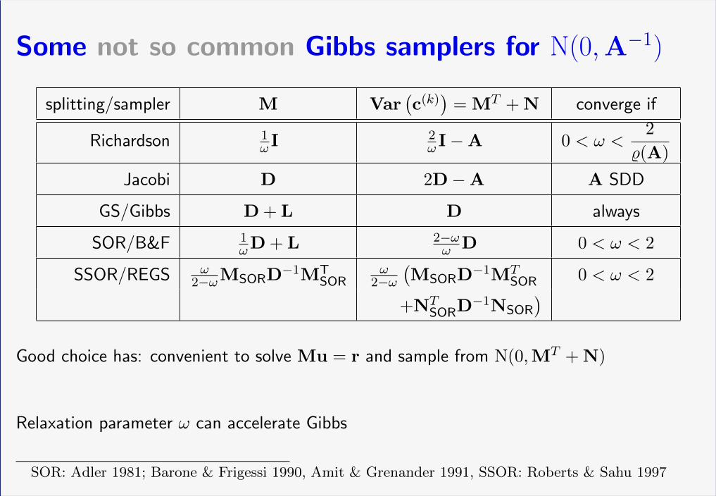
Some not so common Gibbs samplers for N(0,A−1)

splitting/sampler M Var(c(k)

)= MT + N converge if

Richardson 1ω I

2ω I−A 0 < ω <

2

%(A)

Jacobi D 2D−A A SDD

GS/Gibbs D + L D always

SOR/B&F 1ωD + L 2−ω

ω D 0 < ω < 2

SSOR/REGS ω2−ωMSORD

−1MTSOR

ω2−ω

(MSORD

−1MTSOR 0 < ω < 2

+NTSORD

−1NSOR

)Good choice has: convenient to solve Mu = r and sample from N(0,MT + N)

Relaxation parameter ω can accelerate Gibbs

SSOR is a forwards and backwards sweep of SOR to give a symmetric splitting

SOR: Adler 1981; Barone & Frigessi 1990, Amit & Grenander 1991, SSOR: Roberts & Sahu 1997

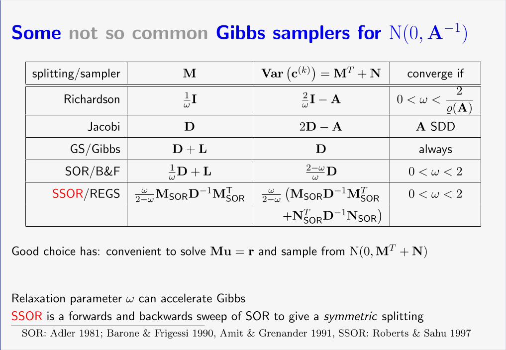
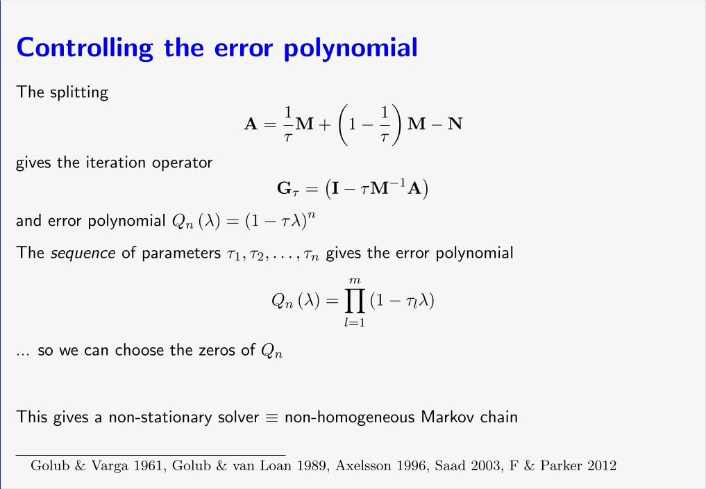
Controlling the error polynomial

The splitting

A =1

τM +

(1− 1

τ

)M−N

gives the iteration operator

Gτ =(I− τM−1A

)and error polynomial Qn (λ) = (1− τλ)n

The sequence of parameters τ1, τ2, . . . , τn gives the error polynomial

Qn (λ) =

m∏l=1

(1− τlλ)

... so we can choose the zeros of Qn

This gives a non-stationary solver ≡ non-homogeneous Markov chain

Golub & Varga 1961, Golub & van Loan 1989, Axelsson 1996, Saad 2003, F & Parker 2012

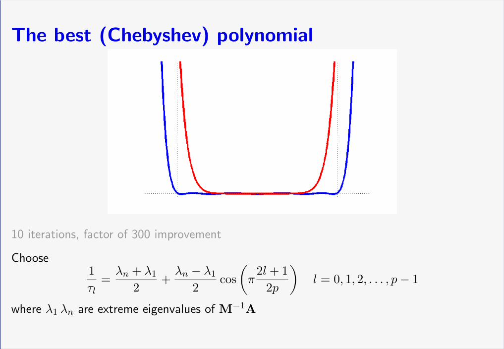
The best (Chebyshev) polynomial

10 iterations, factor of 300 improvement

Choose1

τl=λn + λ1

2+λn − λ1

2cos

(π

2l + 1

2p

)l = 0, 1, 2, . . . , p− 1

where λ1 λn are extreme eigenvalues of M−1A

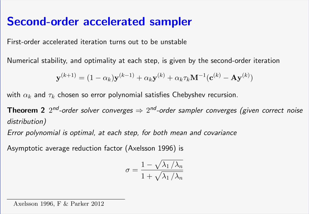
Second-order accelerated sampler

First-order accelerated iteration turns out to be unstable

Numerical stability, and optimality at each step, is given by the second-order iteration

y(k+1) = (1− αk)y(k−1) + αky(k) + αkτkM

−1(c(k) −Ay(k))

with αk and τk chosen so error polynomial satisfies Chebyshev recursion.

Theorem 2 2nd-order solver converges ⇒ 2nd-order sampler converges (given correct noise

distribution)

Error polynomial is optimal, at each step, for both mean and covariance

Asymptotic average reduction factor (Axelsson 1996) is

σ =1−

√λ1 /λn

1 +√λ1 /λn

Axelsson 1996, F & Parker 2012

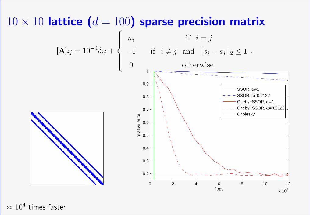
10× 10 lattice (d = 100) sparse precision matrix

[A]ij = 10−4δij +

ni if i = j

−1 if i 6= j and ||si − sj ||2 ≤ 1

0 otherwise

.

0 2 4 6 8 10 12

x 106

0.2

0.3

0.4

0.5

0.6

0.7

0.8

0.9

1

flops

rela

tive

erro

r

SSOR, ω=1

SSOR, ω=0.2122

Cheby−SSOR, ω=1

Cheby−SSOR, ω=0.2122Cholesky

≈ 104 times faster

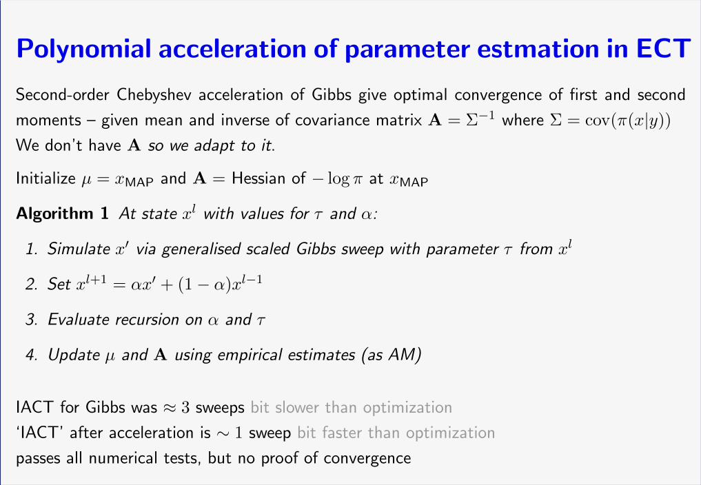
Polynomial acceleration of parameter estmation in ECT

Second-order Chebyshev acceleration of Gibbs give optimal convergence of first and second

moments – given mean and inverse of covariance matrix A = Σ−1 where Σ = cov(π(x|y))

We don’t have A so we adapt to it.

Initialize µ = xMAP and A = Hessian of − log π at xMAP

Algorithm 1 At state xl with values for τ and α:

1. Simulate x′ via generalised scaled Gibbs sweep with parameter τ from xl

2. Set xl+1 = αx′ + (1− α)xl−1

3. Evaluate recursion on α and τ

4. Update µ and A using empirical estimates (as AM)

IACT for Gibbs was ≈ 3 sweeps bit slower than optimization

‘IACT’ after acceleration is ∼ 1 sweep bit faster than optimization

passes all numerical tests, but no proof of convergence

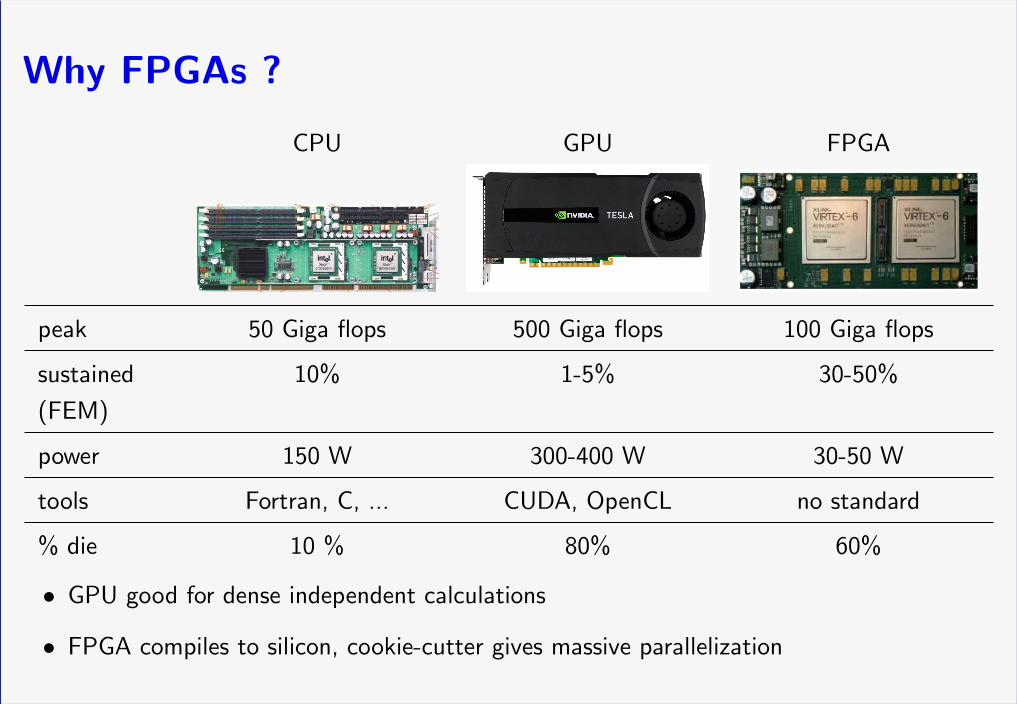
Why FPGAs ?

CPU GPU FPGA

peak 50 Giga flops 500 Giga flops 100 Giga flops

sustained

(FEM)

10% 1-5% 30-50%

power 150 W 300-400 W 30-50 W

tools Fortran, C, ... CUDA, OpenCL no standard

% die 10 % 80% 60%

• GPU good for dense independent calculations

• FPGA compiles to silicon, cookie-cutter gives massive parallelization

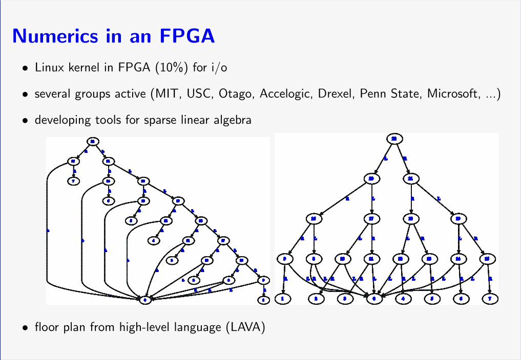
Numerics in an FPGA

• Linux kernel in FPGA (10%) for i/o

• several groups active (MIT, USC, Otago, Accelogic, Drexel, Penn State, Microsoft, ...)

• developing tools for sparse linear algebra

• floor plan from high-level language (LAVA)

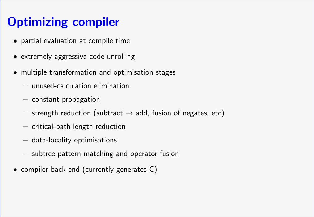
Optimizing compiler

• partial evaluation at compile time

• extremely-aggressive code-unrolling

• multiple transformation and optimisation stages

– unused-calculation elimination

– constant propagation

– strength reduction (subtract → add, fusion of negates, etc)

– critical-path length reduction

– data-locality optimisations

– subtree pattern matching and operator fusion

• compiler back-end (currently generates C)

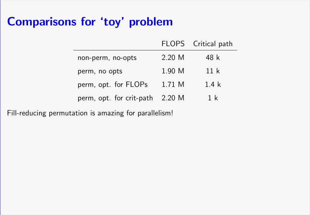
Comparisons for ‘toy’ problem

FLOPS Critical path

non-perm, no-opts 2.20 M 48 k

perm, no opts 1.90 M 11 k

perm, opt. for FLOPs 1.71 M 1.4 k

perm, opt. for crit-path 2.20 M 1 k

Fill-reducing permutation is amazing for parallelism!

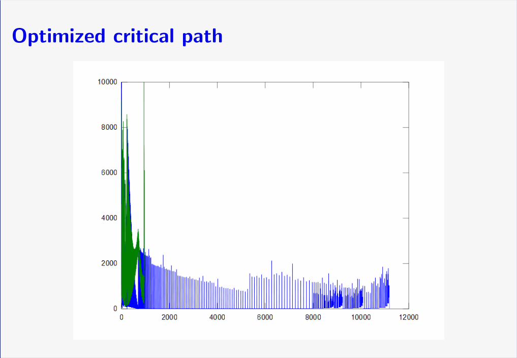
Optimized critical path

Conclusions

• In the Gaussian setting GS ≡ GS

• acceleration of convergence in mean and covariance not limited to Gaussian targets

• Optimizing compiler speeds up calculation by ×30

• FPGA gives another ×10 over parallel CPU

• Multiple conventional CPU per chip also good target

• Looks like real-time embedded UQ is feasible