Monitoring Indirect Contagion∗

PRELIMINARY DRAFT

DO NOT SHARE WITHOUT PERMISSION OF THE AUTHORS.

Rama CONT†, Eric Schaanning‡

May 16, 2018

Abstract

Large overlapping portfolios can become important amplifiers of stress across financial

markets during times of crisis. How can the contagion risk posed by the distressed liqui-

dation of such portfolios be monitored? More generally, how can one quantify the notion

of interconnectedness that common asset holdings create? Our paper introduces two novel

indicators, derived from the network of liquidity-weighted portfolio overlaps, to address these

questions.

The Endogenous Risk Index (ERI) captures spillovers across portfolios in scenarios of

deleveraging and has a natural micro-foundation that arises when accounting for institution-

level losses occurring in a fire sale. The Indirect Contagion Index (ICI) allows to quantify the

degree of “interconnectedness” for systemically important financial institutions’ portfolios by

accounting for the losses that a distressed liquidation would inflict on other portfolios.

Using data on 51 European banks from the European Banking Authority, we show that

our indicators provide valuable information above and beyond the size of banks. These

findings are robust to a wide range of modeling assumptions. Therefore our indicators

may be useful to quantify the degree of “interconnectedness” in the Basel Committee on

Banking Supervision’s Indicator Measurement Approach, as well as contribute to the global

monitoring of contagion channels.

Keywords: Financial stability, price-mediated contagion, macro prudential regulation, sys-

temic risk measurement.

∗The views expressed are those of the authors and do not necessarily reflect those of Norges Bank. Eric

Schaanning’s PhD studies were funded by the Fonds National de la Recherche Luxembourg under the AFR PhD

scheme. We thank seminar and conference participants at the Vienna University of Economics and Business and

the European Systemic Risk Board. Special thanks to Michel Baes, Birgit Rudloff, Martin Summer for stimulating

discussions.

An earlier version of this paper was called “Measuring systemic risk: The indirect contagion index.”†Imperial College London, Department of Mathematics, 180 Queens Gate SW7 2AZ, r.cont@imperial.ac.uk.‡ETH Zurich, RiskLab, Department of Mathematics, Ramistrasse 101, 8092 Zurich, and Norges Bank,

Bankplassen 2, 0151 Oslo. Part of this work was undertaken while Eric Schaanning was at Imperial College

London, eric.schaanning@math.ethz.ch.

1

Contents

1 Introduction 3

2 Monitoring indirect contagion 5

2.1 Fire-sales losses and liquidity-weighted overlaps . . . . . . . . . . . . . . . . . . . 5

2.2 The Endogenous Risk Index. . . . . . . . . . . . . . . . . . . . . . . . . . . . . . 8

2.3 The Indirect Contagion Index . . . . . . . . . . . . . . . . . . . . . . . . . . . . . 9

3 Empirical Application 11

3.1 Data . . . . . . . . . . . . . . . . . . . . . . . . . . . . . . . . . . . . . . . . . . . 11

3.2 Quantifying fire-sales losses with the Endogenous Risk Index. . . . . . . . . . . . 12

3.3 Sensitivity analysis: Scenario composition, market depth and shock intensity. . . 15

3.4 Loss-minimising portfolio deleveraging . . . . . . . . . . . . . . . . . . . . . . . . 18

3.5 Comparison with other measures of overlap. . . . . . . . . . . . . . . . . . . . . . 20

3.6 Quantifying interconnectedness for GSIBs and SIFIs . . . . . . . . . . . . . . . . 23

4 Conclusion 24

A Appendix 29

A.1 EBA data codes . . . . . . . . . . . . . . . . . . . . . . . . . . . . . . . . . . . . 40

2

1 Introduction

How can the notion of interconnectedness that common asset holdings create between insti-

tutions, and SIFIs in particular, be quantified? Which institutions are the most important

propagators of stress in a deleveraging scenario? How can one monitor the risk of contagion

in networks with overlapping portfolio? These are questions that we seek to address in this paper.

There is a rich theoretical literature addressing the analysis of overlapping portfolio networks:

(Ibragimov et al., 2011) shows that diversification that may be optimal from an institution’s in-

dividual point of view can create enormous systemic risks for the system. Their model illustrates

that the optimal social outcome depends critically on the distributional properties of returns,

and in general involves less risk-sharing than would be optimal from an individual perspective.

A similar point is made by (Beale et al., 2011), who quantify in simple models of three to five

assets how the regulator’s preference for portfolio diversity may be at odds with the institutions’

individual preferences for diversification. (Caccioli et al., 2014a) derive asymptotic properties

of deleveraging cascades in bipartite asset-institution networks using Galton-Watson processes.

Highly connected portfolio networks exhibit a “stable yet fragile” behaviour, i.e. contagion is

generally unlikely to occur, but will be catastrophic if it does. (Wagner, 2011) shows that in

the presence of liquidation risks, it is rational for investors to choose heterogeneous portfolios,

i.e. they rationally choose to forgo diversification benefits, so as to reduce the risk of joint

liquidations.

Detailed empirical analyses provide evidence of the effects predicted by theoretical models:

(Khandani and Lo, 2011) trace the substantial losses that a number of funds suffered during

the “Quant event of August 2007” back to the distressed liquidation of a similarly composed

portfolio. (Cont and Wagalath, 2016) go one step further by reverse-engineering the portfolio

that one would have needed to liquidate in order to generate the observed changes in returns,

covariances and eventually losses for similar portfolios. The Quant event of 2007 is thus a text-

book example of price-mediated contagion: institutions that may have no relation to each other

at all suddenly become “indirectly” connected (Cont and Schaanning, 2016). This connection

arises by virtue of their portfolios being composed to varying degrees of the same assets, which

opens the channel for mark to market losses to materialize on all of them simultaneously when

a large market player is forced to liquidate (a part of) its position. (Cont and Wagalath, 2013)

extend the theoretical study by (Pedersen, 2009) to quantify the impact of investors running for

the exit, and the implications for asset returns, in a continuous time setting. At an international

level, (Boyer et al., 2006) and (Jotikasthira et al., 2012) provide strong empirical support for the

spillover effects that asset sales and purchases by large institutional investors can have. (Ellul

et al., 2011) study the forced divestment of downgraded bonds by insurance companies and the

impact on prices. Consistent with the prediction made in (Shleifer and Vishny, 1992), the effects

on prices is all the more important when the buyers (hedge funds in (Ellul et al., 2011)) are

constrained.

A number of measures have been developed to capture these effects more precisely. Indeed,

the growing availability of securities holdings data on various market participants has sparked

3

the interest in analysing systemic risk stemming from overlapping portfolios. Using security-level

holdings data from the German Microdatabase Securities Holdings Statistics, (Timmer, 2016)

provides evidence that banks and investment funds act pro-cyclically to price changes (they sell

when prices fall and buy when prices rise), while insurance companies and pension funds act

counter-cyclically. (Guo et al., 2015) analyse the topology of common holdings in the US fund

industry and find that greater overlap contributes to greater negative excess returns in the pres-

ence of liquidations. Similarly, (Braverman and Minca, 2016) use a similar network of portfolio

overlaps to derive three measures of vulnerability which are shown to correlate significantly with

negative returns of funds under stress. The measures of indirect contagion that we introduce

in this paper are using similar building blocks as the measures of vulnerability in (Braverman

and Minca, 2016). Moreover, by relating it to the deleveraging model introduced in (Cont and

Schaanning, 2016) we provide a micro-foundation for our measure of indirect contagion.

(Getmansky et al., 2016) introduce “cosine-similarity” (the scalar product of two portfolio’s

weights) as a measure of similarity between portfolios. Their study shows that insurance com-

panies with a higher measure of commonality tend to engage in larger common sales, regardless

of portfolio size. We will compare our measures of indirect contagion in detail to cosine similar-

ity, and other overlap measures. (Blei and Bakhodir, 2014) use clustering tools from machine

learning to infer an ”Asset Commonality” measure of risk (ACRISK). The measure quantifies

the degree of commonality between large portfolios and captures the build-up of systemic risk

several years prior to the crisis.

(Kritzman et al., 2011), who use the degree of variation explained by the first principal com-

ponent of asset returns as a measure of systemic risk in markets, constitutes an intermediate

step between the exposure-based measures described above and market-based measures of sys-

temic risk. Among the most widely used market-based measures are “∆ CoVaR”(Adrian and

Brunnermeier, 2016), “SRISK” (Brownlees and Engle, 2016), and the Marginal Expected Short-

fall “(Acharya et al., 2017). These measures are constructed from a statistical analysis of the

equity returns of listed companies, and are meant to aggregate many risk facets, as priced by the

market, rather than focus specifically on overlapping portfolios. SRISK for instance measures

the capital shortfall of a firm conditional on a severe market decline and depends on the firms

size, leverage and risk. While not being based on actual exposures (and thus potential future

losses), such measures aggregate market perceptions of risk into a number, and can function

well as thermometers of risk. (Bisias et al., 2012) provides a comprehensive overview of different

systemic risk measures.

By building on actual portfolio holdings, the contagion measures introduced in this paper

function rather like a barometer of risk, quantifying “pressure” in the sense of the potential for

future losses. The upside of our approach is that it allows to uncover risks that are not priced

by the market because portfolio holdings are confidential and this risk cannot be priced in the

market. The downside is of course that a sophisticated implementation of the methodology

requires access to such confidential securities holding data. However, as part of the post-crisis

reform package, such securities holdings data is currently being collected, which thus allows

these analyses to be performed in the future.1

1See e.g. https://www.ecb.europa.eu/stats/financial_markets_and_interest_rates/securities_

holdings/html/index.en.html

4

Main contributions.

1. Endogenous Risk Index: Given portfolio holdings data, we construct a network of

indirect contagion which is based on the overlap of institutions’ portfolios, adjusted for

the liquidity of the underlying assets. We introduce the Endogenous Risk Index (ERI),

the Perron-eigenvector of this liquidity-weighted overlap matrix of portfolios, and show

that it has a natural micro-foundation that comes from correctly quantifying mark to

market losses in deleveraging scenarios. The ERI is shown to be a good proxy of spillover

losses over and above the size of portfolios. In particular, accounting for the liquidity of

the underlying assets in the portfolio improves the prediction of fire sales losses markedly.

The ERI can function as a proxy for monitoring contagion in periods between stress tests.

2. Indirect Contagion Index: The Indirect Contagion Index (ICI) is a modified version

of the Endogenous Risk Index, which ignores self-inflicted liquidation losses and stresses

losses caused to other portfolios. In the framework of the Basel Committee on Banking

Supervision’s GSIB methodology the ICI could be used as an additional indicator to

quantify the degree of interconnectedness of systemically important institutions. Using

data from the 2016 EBA stress test, we find that relating to the price-mediated contagion

channel, Credit Agricole, Deutsche Bank, BNP Paribas, Societe Generale and Barclays are

among the most systemic institutions.

The predictive power of our indicators is robust to a wide range of modeling assumptions such

as the liquidation strategies which institutions use to delever portfolios, or the scenarios that

trigger these.

Structure. The paper is organised as follows: Section 2.1 is devoted introduces our framework

to monitor indirect contagion. Section 2.2 and 2.3 present the Endogenous Risk Index and the

Indirect Contagion Index respectively. Sections 3.1 and 3.2 apply our methodology to a dataset

of European Banks. Moreover, we perform a large sensitivity analysis in Section 3.3. and

introduce an optimal bank response in Section 3.4. Section 3.5 compares the ERI and ICI to

other measures of overlap, while Section 3.6 suggests an application of the indicators to monitor

Global Systemically Important Banks (GSIBs) in the Basel Committe on Banking Supervisions’

framework. Section 4 concludes.

2 Monitoring indirect contagion

2.1 Fire-sales losses and liquidity-weighted overlaps

We consider a financial network consisting of i = 1..N institutions and µ = 1..M securities. The

institutions are subject to regulatory, market- or self-imposed constraints, which may depend

on their capital, leverage or liquidity levels. Let Πi,µ denote the value of institution i’s holdings

in asset class µ in monetary units. The portfolio holdings of the entire system are given by the

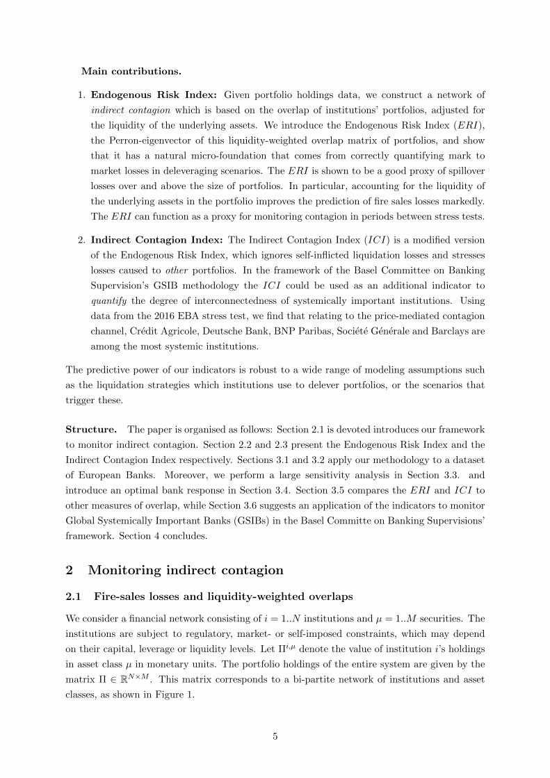
matrix Π ∈ RN×M . This matrix corresponds to a bi-partite network of institutions and asset

classes, as shown in Figure 1.

5

Figure 1: Bipartite network of institutions A-K and asset classes 1-4, which gives rise to anetwork of indirect contagion between institutions.

Such a network can give rise to indirect contagion: Even though institutions A through E

may have no connection, institutions B to E may suffer losses if for some reason A is forced to

liquidate its position in asset class 1, thereby depressing its price. Specifically, two types of losses

can arise: (i) mark-to-market losses on remaining holdings, suffered by all parties that hold the

asset undergoing the distressed liquidation and (ii) implementation costs which the liquidating

institution suffers on the position it is trying to liquidate. Moreover, if, as a result of the forced

deleveraging by A, institutions B or D need to liquidate a part of their portfolio, the price of

asset class 2 may drop and cause losses for institutions F and G, who were previously unaffected.

This shows how overlapping portfolios can become a driver of cross-asset class contagion, even

when the asset classes are economically and geographically essentially independent.

In order to quantify this phenomenon properly, we need to specify: (i) when institutions react to

a shock, (i) how they react when forced to, and (iii) how prices respond to forced liquidations.

Using these three building blocks, we show that an endogenous risk index naturally arises when

one quantifies the liquidation losses in such a network of constrained and overlapping portfolios.

The presentation follows the model discussion in Cont and Schaanning (2016), to which we

refer the reader for further details:

1. At time k = 1, in response to a stress scenario, parametrised by percentage shocks to asset

classes ε ∈ [0, 1]M , some institutions j deleverage their portfolio by selling a proportion

Γjk(ε) ∈ [0, 1] of marketable assets. In Section 3.4, we assume that banks do not sell assets

proportionately, but choose Γj so as to minimise the liquidation losses they suffer. This

leads to an aggregate amount qµk =∑N

j=1 Πj,µk−1Γjk(ε) of sales in asset class µ. In general, the

deleveraging proportion, Γjk(ε) can depend on the capital buffer, the liquidity reserves and

other balance sheet components of institution j. In particular, when j is well-capitalised

and has a prudent liquidity buffer, it will be able to withstand the shock without resorting

to distressed liquidations, in which case Γj(ε) = 0. We specify Γ precisely in the empirical

6

section and will drop the ε in Γ(ε) for notational convenience.

2. The market price of asset class µ is denoted by Sµk . The impact of asset sales results in a

decline of the market price, moving it to

Sµk = Sµk−1

(1−

qµkDµ

), (1)

where the market depth Dµ(τ) ∝ ADVµσµ

√τ is proportional to the ratio of the average

daily volume (ADV) and the volatility of the asset class times the liquidation horizon, τ ,

which is assumed to be τ = 20 days in our calibration. This corresponds to a linear price

impact function ∆SS = −Ψµ(x) := x

Dµ, as used in ((Obizhaeva, 2012), (Kyle and Obizhaeva,

2016), (Amihud, 2002), (Cont and Wagalath, 2016)). For a more general discussion on

non-linear price impact functions in the context of stress testing, we refer to (Cont and

Schaanning, 2016).

3. For any institution i, the combined effect of its own deleveraging (if it occurs) and the

impact of other forced sales changes the market value of its holdings in asset class µ to

Πi,µk =

(1− Γik

)︸ ︷︷ ︸Remainder after deleveraging by i

Previous value︷ ︸︸ ︷Πi,µk−1

1−D−1µ

N∑j=1

ΓjkΠj,µk−1

︸ ︷︷ ︸

Price impact on remaining holdings

. (2)

Importantly, this shows that in general the value of institution i’s holdings under stress

cannot be simply inferred from historically observed returns and covariances, but may

depend on the stress scenario and the network of overlapping portfolios.

The price move generates two types of losses for portfolio i: First, it causes mark to market

losses on the remaining part of the portfolio given by

M ik =

M∑µ=1

((1− Γik)Π

i,µk−1 −Πi,µ

k

)= (1− Γik)

M∑µ=1

Πi,µk−1D

−1µ

N∑j=1

ΓjkΠj,µk−1

= (1− Γik)

N∑j=1

M∑µ=1

Πi,µk−1Πj,µ

k−1

DµΓjk. (3)

A second source of loss stems from the fact that assets are not liquidated at the current market

price but at a discount. We assume for simplicity that the deleveraging institutions suffer the

same price impact on the liquidated part of the portfolio as on their remaining part, yielding

the realised loss

Rik =M∑µ=1

(ΓikΠ

i,µk−1 − ΓikΠ

i,µk−1

(1−

qµkDµ

))

= Γik

N∑j=1

M∑µ=1

Πi,µk−1Πj,µ

k−1

DµΓjk. (4)

7

Summing (4) and (3) yields the total loss of portfolio i at the k-th round of deleveraging:

Lik =N∑j=1

M∑µ=1

Πi,µk−1Πj,µ

k−1

Dµ︸ ︷︷ ︸Ωij(Πk−1)

Γjk =N∑j=1

Ωijk−1Γjk,

which shows that the magnitude of fire sales spillovers from institution i to institution j is

proportional to the liquidity-weighted overlap Ωij between portfolios i and j (Cont and Wagalath,

2013):

Ωij(Πk) :=

M∑µ=1

Πi,µk Πj,µ

k

Dµ.

Let D := diag(D1, . . . , DM ), then the matrix of portfolio overlaps

Ω(Πk) = ΠkD−1Π>k , (5)

can be viewed as a (liquidity-)weighted adjacency matrix of the network linking portfolios

through their common holdings.

2.2 The Endogenous Risk Index.

From the derivation above, it follows that in the first round, the fire-sales losses for all banks

are given by the vector

FLoss = ΩΓ. (6)

As Ω is symmetric positive semi-definite by construction, we know that there exists an or-

thonormal basis of eigenvectors with real eigenvalues for it. We further assume that Ω is an

irreducible and non-negative matrix. This is equivalent to the network of overlapping portfolios

being strongly connected (i.e. it is not a union of disjoint sub-networks) and that there are no

pairs of portfolios such that∑M

µ=1Πi,µΠj,µ

Dµ< 0 respectively. The European banking network

which we use in our empirical analysis verifies these assumptions. Under these conditions, the

Perron-Frobenius theorem ensures that the components of the first eigenvector are all positive.

If the first eigenvalue dominates, the network of liquidity-weighted portfolio overlaps can be

approximated well by a one-factor model

Ω ≈ λ1uu>, (7)

where u is the Perron eigenvector corresponding to the largest eigenvalue λ1. Using this approx-

imation, the fire-sales loss can be written as

FLossi = λ1ui

N∑j=1

ujΓj(ε).

8

Taking logarithms, we get

log(FLossi) = log(λ1ui

N∑j=1

ujΓj(ε))

= 1×︸︷︷︸slope

log(ui) + log(λ1) + log(u>Γ(ε)),︸ ︷︷ ︸Intercept

(8)

which implies that the logarithm of the Perron eigenvector should be a good predictor of fire-sales

losses. Moreover, we should expect a slope of approximately one when regressing log-fire-sales

losses on it.

Equation (8) motivates the introduction of the following definition: The Endogenous Risk

Index (ERI) of a financial institution is its component i in the Perron eigenvector ui of the

matrix Ω from (5) of liquidity-weighted portfolio overlaps:

ERI(i) = ui. (9)

The EIR provides a measure of centrality of the node i in the network whose links are weighted

by the overlap matrix Ω. The ERI is constructed as follows:

1. Collect portfolio holdings Πi,µ by asset class for each financial institution in the network,

at the granularity level corresponding to bank stress tests.

2. Estimate a market depth parameter Dµ ∝ ADVµσµ

for each asset class.

3. Check that Ωij ≥ 0 and that Ω is irreducible.

4. Compute the largest eigenvalue and the corresponding eigenvector (the “Perron eigenvec-

tor”) u = (ui, i = 1...N) of the matrix of liquidity-weighted overlaps Ω(Π) = ΠD−1Π>.

5. The Endogenous Risk Index is the Perron eigenvector, ERI = u.

2.3 The Indirect Contagion Index

Before turning to the empirical application, we propose a modification relative to the ERI that

discounts the fire-sales losses that a distressed portfolio liquidation would inflict on itself, and

only take into consideration the spillover-losses that are generated to other portfolios. We call

this measure the Indirect Contagion Index (ICI), and compute it as follows:

1. Compute Ω = ΠD−1Π>, as detailed for the ERI above.

2. Compute the largest eigenvalue and the corresponding Perron eigenvector v of

Ω0 := Ω− diag(Ω11, . . . ,ΩNN ).2

3. The Indirect Contagion Index is the Perron eigenvector, ICI = v.

2Note that the zero diagonal of Ω0 does not make the matrix reducible or violate the non-negativity constraint,and hence the Perron-Frobenius Theorem is still applicable.

9

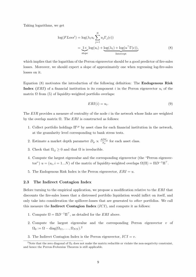
We illustrate the difference between the ERI and the ICI, in a simple financial network of 7

banks and 2 asset classes given by:

Π =

(1000 0 0 0 0 0 0

100 1100 100 100 100 100 100

)>D = (1000, 2000)>.

Banks 1 and 2 are thus large (and equal in size), while banks 3 - 7 are smaller. Asset class 1 is

twice as illiquid as asset class 2. The left panel of Figure 2 shows the network, where the blue

squares denote banks, the red circles denote asset classes and the size of the edge denotes the

magnitude of the holding (not to scale). The bigger banks are denoted by larger squares; the

more illiquid asset class is depicted by a larger circle. The right panel of Figure 2 shows the ICI

(blue bars) and the ERI (black crosses) for this network. Bank 1 clearly dominates the ERI

ranking. This is due to its main holdings being less liquid compared to Bank 2’s holdings, and

the amount of self-contagion that this could trigger. In contrast, Bank 2 has a large position

in asset class 2, which all the medium-sized banks hold as well. Consequently, even though the

same liquidation volume for Bank 2 in asset class 2 would cause a smaller loss than it would

for Bank 1 in asset class 1, if Bank 2 delevers, the rest of the system also suffers significant

fire-sales losses. The ICI discounts the self-inflicted fire-sales loss and only accounts for system

externalities, which is why in the ICI ranking, Bank 2 dominates, and Bank 1 is equally ranked

as the medium-sized banks.

A B

1 2 3 4 5 6 7 1 2 3 4 5 6 7

0.0

0.2

0.4

0.6

0.8

1.0

Bank

ER

I and

ICI

ICIERI

Figure 2: Illustrative example showing how the ICI discounts self-inflicted losses compared tothe losses caused for other participants relative to the ERI.

We will further discuss the difference between the ERI and the ICI for European banks in

the sections below.

10

3 Empirical Application

3.1 Data

We use data from the 2016 stress test exercise by the European Banking Authority (EBA)

which provides information on notional exposures of 51 European banks across several hundred

asset classes.3 Holdings are disaggregated by asset type and geographical region. We subdivide

marketable assets into corporate and sovereign bonds, which may be liquidated in a stress

scenario. All other asset classes are classified as illiquid assets and assumed to be unavailable

for short-term liquidations (non-securitised exposures). Ignoring asset classes to which the

European banking system, as a whole, has an exposure below 1M EUR, leaves us with 93 asset

classes, yielding a 51×93 matrix of liquid holdings Π. The most important regions for corporate

exposures, covering over 75% of the total, are France (21.0%), U.S. (14.1%), Germany (11.7%),

Italy (6.5%), Spain (4.6%), Netherlands (4.4%) and Belgium (3.2%). The most important

regions for sovereign exposures, covering more than 75% of the total, are Germany (13.8 %),

France (13.3%), U.S. (12.8%), Italy (9.2%), U.K. (8.4%), Spain (6.3%), Netherlands (4.6%),

Belgium (4.2 %) and Japan (3.4%). Through a similar procedure, we obtain a 51× 98 matrix of

illiquid holdings, which we denote Θ. This corresponds to 97 asset classes for commercial and

residential mortgage exposures respectively in the various regions and a 98th entry consisting of

all remaining illiquid asset holdings (intangible goods, defaulted exposures etc).

Collectively, the 51 banks hold assets totalling 26.3 trillion EUR, of which 54.6 % (14.3 tn

EUR) are in loans and advances, 31.1 % (8.2 tn EUR) are in marketable assets, and 14.3 % (3.8

tn EUR) are in “residual” assets classes that are not of relevance for our model.

The market depth parameter Dµ defined in (1) is computed following the methodology in

(Obizhaeva, 2012) and (Cont and Schaanning, 2016). The estimation procedure is explained in

more detail in Section 3.3, where we perform a sensitivity analysis on this parameter.

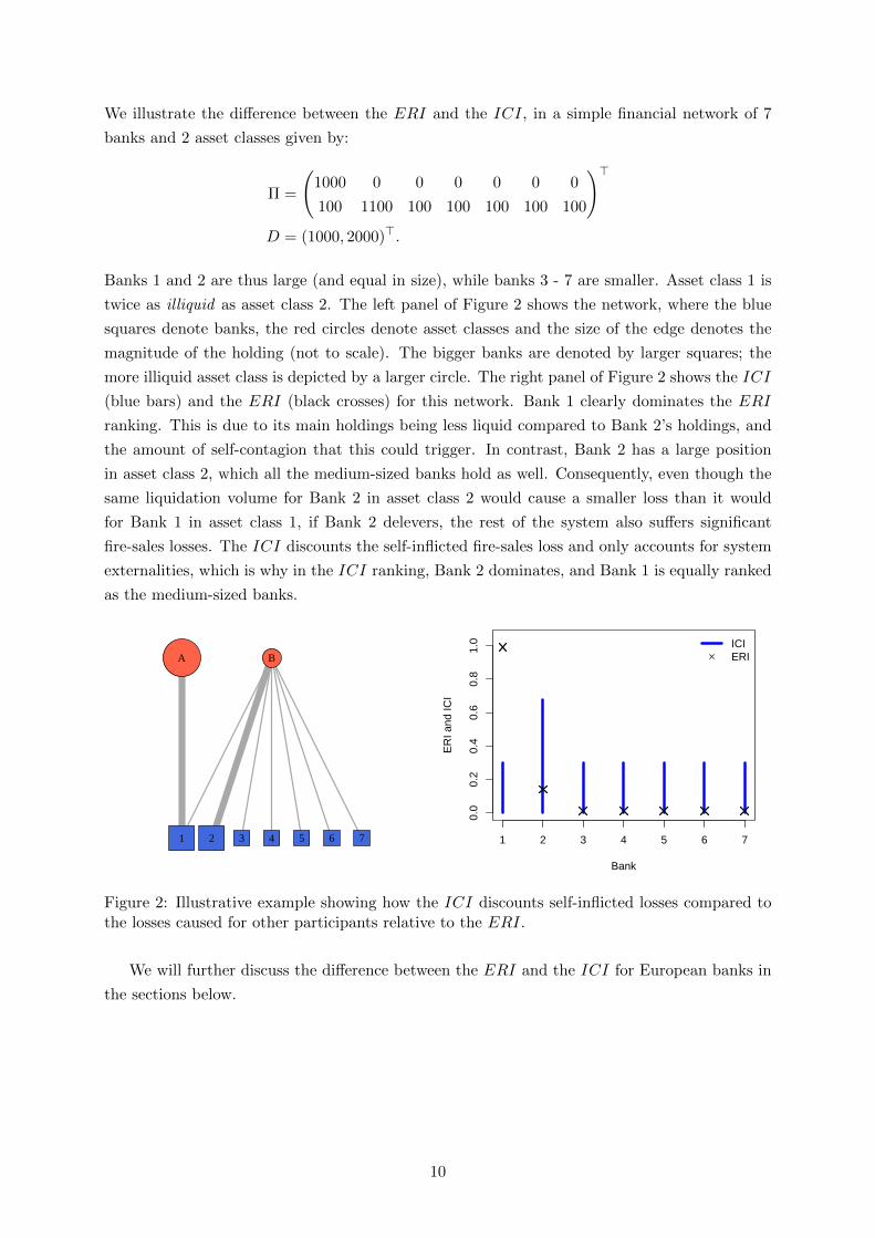
Empirical analysis. As the portfolio holdings from the 2016 EBA data fulfil all our assump-

tions, we compute Ω as well as the ERI and ICI as detailed above. The left-hand panel of

Figure 3 shows that the distribution of liquidity-weighted overlaps Ωij displays considerable het-

erogeneity. The right panel shows the first twenty ranked eigenvalues of Ω. The first eigenvalue

accounts for about 65% of the total variation and clearly dominates the remaining ones, we thus

expect the ERI to be a good predictor of fire-sales losses in the sequel.

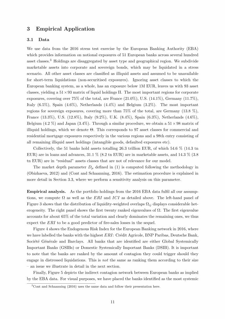
Figure 4 shows the Endogenous Risk Index for the European Banking network in 2016, where

we have labelled the banks with the highest ERI: Credit Agricole, BNP Paribas, Deutsche Bank,

Societe Generale and Barclays. All banks that are identified are either Global Systemically

Important Banks (GSIBs) or Domestic Systemically Important Banks (DSIB). It is important

to note that the banks are ranked by the amount of contagion they could trigger should they

engage in distressed liquidations. This is not the same as ranking them according to their size

– an issue we illustrate in detail in the next section.

Finally, Figure 5 depicts the indirect contagion network between European banks as implied

by the EBA data. For visual purposes, we have placed the banks identified as the most systemic

3Cont and Schaanning (2016) uses the same data and follow their presentation here.

11

Liquidity−weighted overlap (EUR)

Per

cent

02

46

812

0 10 102103104105106107108109101010111012

5 10 15 20

010

2030

4050

60

Ranked eigenvalues

% o

f var

iatio

n

Figure 3: Distribution of liquidity-weighted overlaps (left) and the ranked eigenvalues of theindirect contagion network.

0 10 20 30 40 50

0.0

0.1

0.2

0.3

0.4

0.5

0.6

Bank

ER

I

Deutsche BNP

C.A.

Soc.Gen.

Barclays

Countries

ESDEFRGB/IEITNO/SE/DK/FIPT/GROther

Figure 4: The Endogenous Risk Index for the European Banking system. (Data: EBA. Calcu-lations: Authors).

by the ERI in the centre, and coloured edges orange that connect these banks with each other

as well as with other banks.

3.2 Quantifying fire-sales losses with the Endogenous Risk Index.

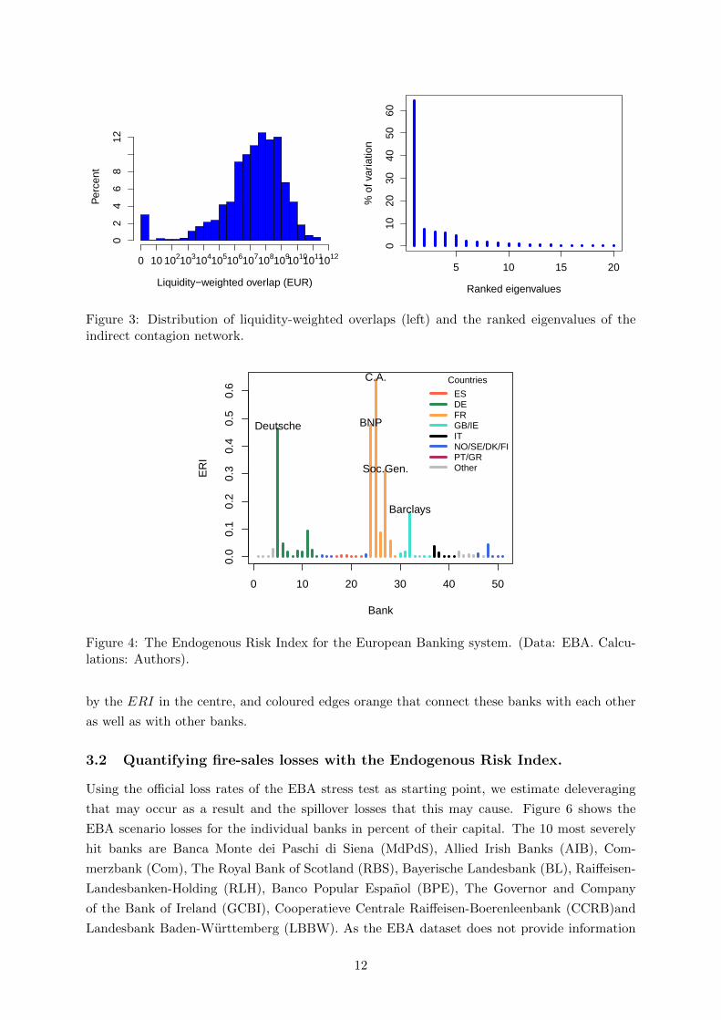
Using the official loss rates of the EBA stress test as starting point, we estimate deleveraging

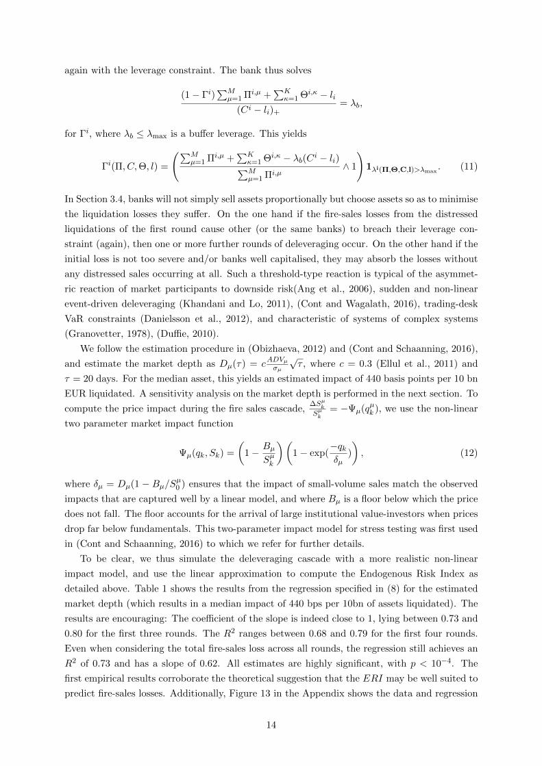
that may occur as a result and the spillover losses that this may cause. Figure 6 shows the

EBA scenario losses for the individual banks in percent of their capital. The 10 most severely

hit banks are Banca Monte dei Paschi di Siena (MdPdS), Allied Irish Banks (AIB), Com-

merzbank (Com), The Royal Bank of Scotland (RBS), Bayerische Landesbank (BL), Raiffeisen-

Landesbanken-Holding (RLH), Banco Popular Espanol (BPE), The Governor and Company

of the Bank of Ireland (GCBI), Cooperatieve Centrale Raiffeisen-Boerenleenbank (CCRB)and

Landesbank Baden-Wurttemberg (LBBW). As the EBA dataset does not provide information

12

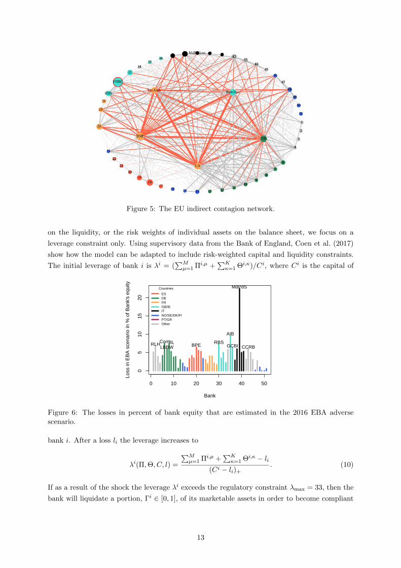
Figure 5: The EU indirect contagion network.

on the liquidity, or the risk weights of individual assets on the balance sheet, we focus on a

leverage constraint only. Using supervisory data from the Bank of England, Coen et al. (2017)

show how the model can be adapted to include risk-weighted capital and liquidity constraints.

The initial leverage of bank i is λi = (∑M

µ=1 Πi,µ +∑K

κ=1 Θi,κ)/Ci, where Ci is the capital of

0 10 20 30 40 50

05

1015

20

Bank

Loss

in E

BA

sce

nario

in %

of B

ank'

s eq

uity

MdPdS

AIB

Com RBSBLRLH BPE GCBI CCRBLBBW

Countries

ESDEFRGB/IEITNO/SE/DK/FIPT/GROther

Figure 6: The losses in percent of bank equity that are estimated in the 2016 EBA adversescenario.

bank i. After a loss li the leverage increases to

λi(Π,Θ, C, l) =

∑Mµ=1 Πi,µ +

∑Kκ=1 Θi,κ − li

(Ci − li)+. (10)

If as a result of the shock the leverage λi exceeds the regulatory constraint λmax = 33, then the

bank will liquidate a portion, Γi ∈ [0, 1], of its marketable assets in order to become compliant

13

again with the leverage constraint. The bank thus solves

(1− Γi)∑M

µ=1 Πi,µ +∑K

κ=1 Θi,κ − li(Ci − li)+

= λb,

for Γi, where λb ≤ λmax is a buffer leverage. This yields

Γi(Π, C,Θ, l) =

(∑Mµ=1 Πi,µ +

∑Kκ=1 Θi,κ − λb(Ci − li)∑Mµ=1 Πi,µ

∧ 1

)1λi(Π,Θ,C,l)>λmax

. (11)

In Section 3.4, banks will not simply sell assets proportionally but choose assets so as to minimise

the liquidation losses they suffer. On the one hand if the fire-sales losses from the distressed

liquidations of the first round cause other (or the same banks) to breach their leverage con-

straint (again), then one or more further rounds of deleveraging occur. On the other hand if the

initial loss is not too severe and/or banks well capitalised, they may absorb the losses without

any distressed sales occurring at all. Such a threshold-type reaction is typical of the asymmet-

ric reaction of market participants to downside risk(Ang et al., 2006), sudden and non-linear

event-driven deleveraging (Khandani and Lo, 2011), (Cont and Wagalath, 2016), trading-desk

VaR constraints (Danielsson et al., 2012), and characteristic of systems of complex systems

(Granovetter, 1978), (Duffie, 2010).

We follow the estimation procedure in (Obizhaeva, 2012) and (Cont and Schaanning, 2016),

and estimate the market depth as Dµ(τ) = cADVµσµ

√τ , where c = 0.3 (Ellul et al., 2011) and

τ = 20 days. For the median asset, this yields an estimated impact of 440 basis points per 10 bn

EUR liquidated. A sensitivity analysis on the market depth is performed in the next section. To

compute the price impact during the fire sales cascade,∆SµkSµk

= −Ψµ(qµk ), we use the non-linear

two parameter market impact function

Ψµ(qk, Sk) =

(1− Bµ

Sµk

)(1− exp(

−qkδµ

)

), (12)

where δµ = Dµ(1 − Bµ/Sµ0 ) ensures that the impact of small-volume sales match the observed

impacts that are captured well by a linear model, and where Bµ is a floor below which the price

does not fall. The floor accounts for the arrival of large institutional value-investors when prices

drop far below fundamentals. This two-parameter impact model for stress testing was first used

in (Cont and Schaanning, 2016) to which we refer for further details.

To be clear, we thus simulate the deleveraging cascade with a more realistic non-linear

impact model, and use the linear approximation to compute the Endogenous Risk Index as

detailed above. Table 1 shows the results from the regression specified in (8) for the estimated

market depth (which results in a median impact of 440 bps per 10bn of assets liquidated). The

results are encouraging: The coefficient of the slope is indeed close to 1, lying between 0.73 and

0.80 for the first three rounds. The R2 ranges between 0.68 and 0.79 for the first four rounds.

Even when considering the total fire-sales loss across all rounds, the regression still achieves an

R2 of 0.73 and has a slope of 0.62. All estimates are highly significant, with p < 10−4. The

first empirical results corroborate the theoretical suggestion that the ERI may be well suited to

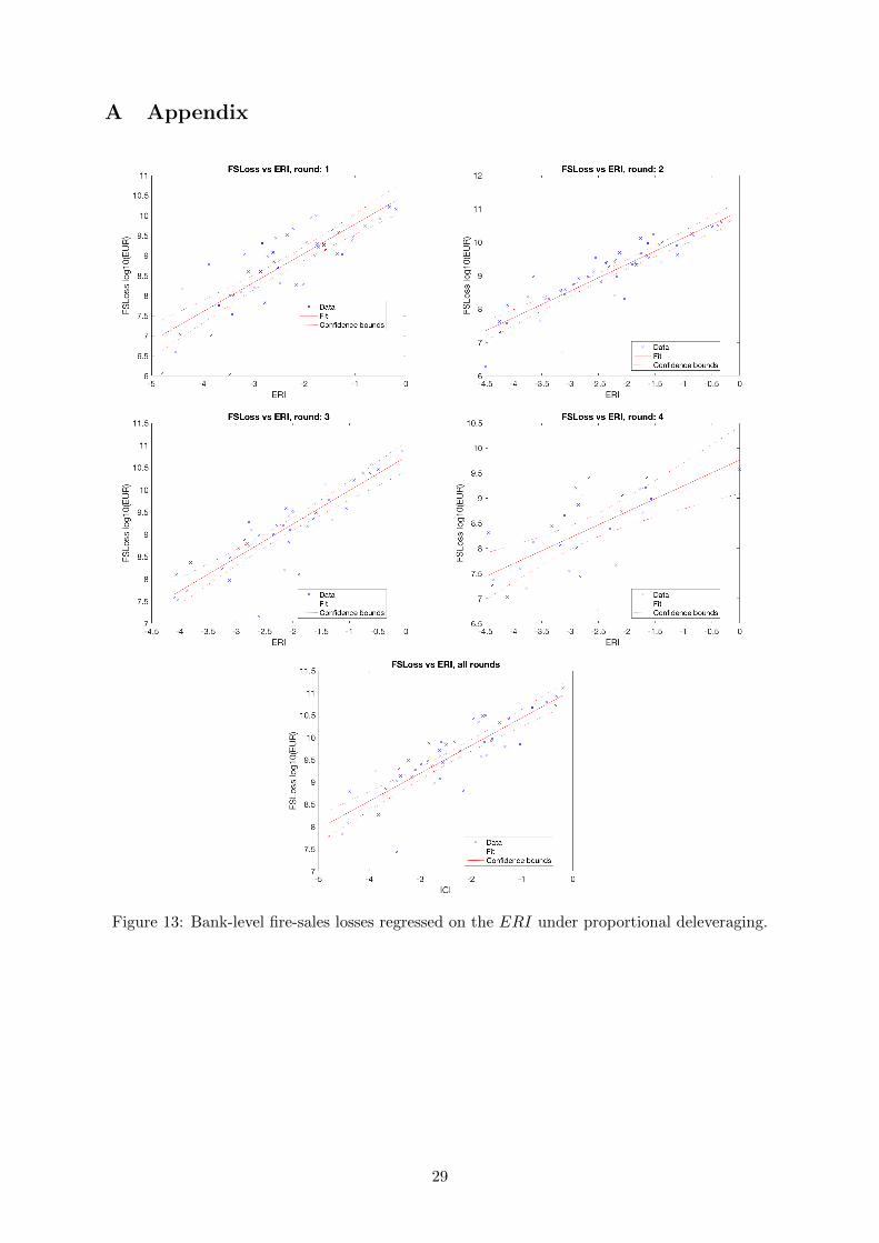
predict fire-sales losses. Additionally, Figure 13 in the Appendix shows the data and regression

14

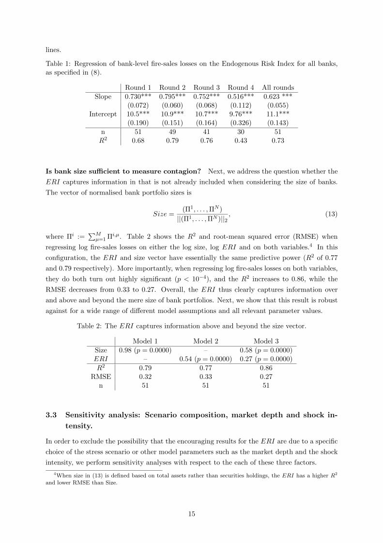
lines.

Table 1: Regression of bank-level fire-sales losses on the Endogenous Risk Index for all banks,as specified in (8).

Round 1 Round 2 Round 3 Round 4 All rounds

Slope 0.730*** 0.795*** 0.752*** 0.516*** 0.623 ***(0.072) (0.060) (0.068) (0.112) (0.055)

Intercept 10.5*** 10.9*** 10.7*** 9.76*** 11.1***(0.190) (0.151) (0.164) (0.326) (0.143)

n 51 49 41 30 51R2 0.68 0.79 0.76 0.43 0.73

Is bank size sufficient to measure contagion? Next, we address the question whether the

ERI captures information in that is not already included when considering the size of banks.

The vector of normalised bank portfolio sizes is

Size =(Π1, . . . ,ΠN )

||(Π1, . . . ,ΠN )||2, (13)

where Πi :=∑M

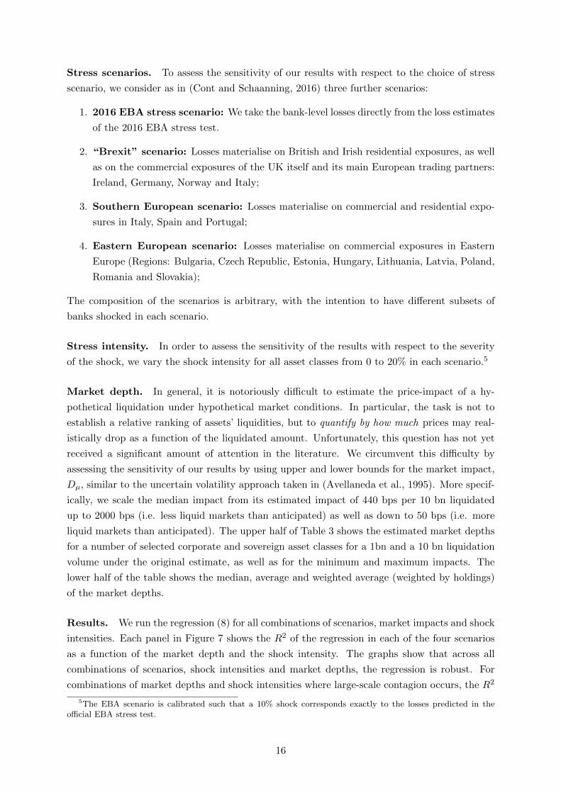
µ=1 Πi,µ. Table 2 shows the R2 and root-mean squared error (RMSE) when

regressing log fire-sales losses on either the log size, log ERI and on both variables.4 In this

configuration, the ERI and size vector have essentially the same predictive power (R2 of 0.77

and 0.79 respectively). More importantly, when regressing log fire-sales losses on both variables,

they do both turn out highly significant (p < 10−4), and the R2 increases to 0.86, while the

RMSE decreases from 0.33 to 0.27. Overall, the ERI thus clearly captures information over

and above and beyond the mere size of bank portfolios. Next, we show that this result is robust

against for a wide range of different model assumptions and all relevant parameter values.

Table 2: The ERI captures information above and beyond the size vector.

Model 1 Model 2 Model 3

Size 0.98 (p = 0.0000) – 0.58 (p = 0.0000)ERI – 0.54 (p = 0.0000) 0.27 (p = 0.0000)

R2 0.79 0.77 0.86RMSE 0.32 0.33 0.27

n 51 51 51

3.3 Sensitivity analysis: Scenario composition, market depth and shock in-

tensity.

In order to exclude the possibility that the encouraging results for the ERI are due to a specific

choice of the stress scenario or other model parameters such as the market depth and the shock

intensity, we perform sensitivity analyses with respect to the each of these three factors.

4When size in (13) is defined based on total assets rather than securities holdings, the ERI has a higher R2

and lower RMSE than Size.

15

Stress scenarios. To assess the sensitivity of our results with respect to the choice of stress

scenario, we consider as in (Cont and Schaanning, 2016) three further scenarios:

1. 2016 EBA stress scenario: We take the bank-level losses directly from the loss estimates

of the 2016 EBA stress test.

2. “Brexit” scenario: Losses materialise on British and Irish residential exposures, as well

as on the commercial exposures of the UK itself and its main European trading partners:

Ireland, Germany, Norway and Italy;

3. Southern European scenario: Losses materialise on commercial and residential expo-

sures in Italy, Spain and Portugal;

4. Eastern European scenario: Losses materialise on commercial exposures in Eastern

Europe (Regions: Bulgaria, Czech Republic, Estonia, Hungary, Lithuania, Latvia, Poland,

Romania and Slovakia);

The composition of the scenarios is arbitrary, with the intention to have different subsets of

banks shocked in each scenario.

Stress intensity. In order to assess the sensitivity of the results with respect to the severity

of the shock, we vary the shock intensity for all asset classes from 0 to 20% in each scenario.5

Market depth. In general, it is notoriously difficult to estimate the price-impact of a hy-

pothetical liquidation under hypothetical market conditions. In particular, the task is not to

establish a relative ranking of assets’ liquidities, but to quantify by how much prices may real-

istically drop as a function of the liquidated amount. Unfortunately, this question has not yet

received a significant amount of attention in the literature. We circumvent this difficulty by

assessing the sensitivity of our results by using upper and lower bounds for the market impact,

Dµ, similar to the uncertain volatility approach taken in (Avellaneda et al., 1995). More specif-

ically, we scale the median impact from its estimated impact of 440 bps per 10 bn liquidated

up to 2000 bps (i.e. less liquid markets than anticipated) as well as down to 50 bps (i.e. more

liquid markets than anticipated). The upper half of Table 3 shows the estimated market depths

for a number of selected corporate and sovereign asset classes for a 1bn and a 10 bn liquidation

volume under the original estimate, as well as for the minimum and maximum impacts. The

lower half of the table shows the median, average and weighted average (weighted by holdings)

of the market depths.

Results. We run the regression (8) for all combinations of scenarios, market impacts and shock

intensities. Each panel in Figure 7 shows the R2 of the regression in each of the four scenarios

as a function of the market depth and the shock intensity. The graphs show that across all

combinations of scenarios, shock intensities and market depths, the regression is robust. For

combinations of market depths and shock intensities where large-scale contagion occurs, the R2

5The EBA scenario is calibrated such that a 10% shock corresponds exactly to the losses predicted in theofficial EBA stress test.

16

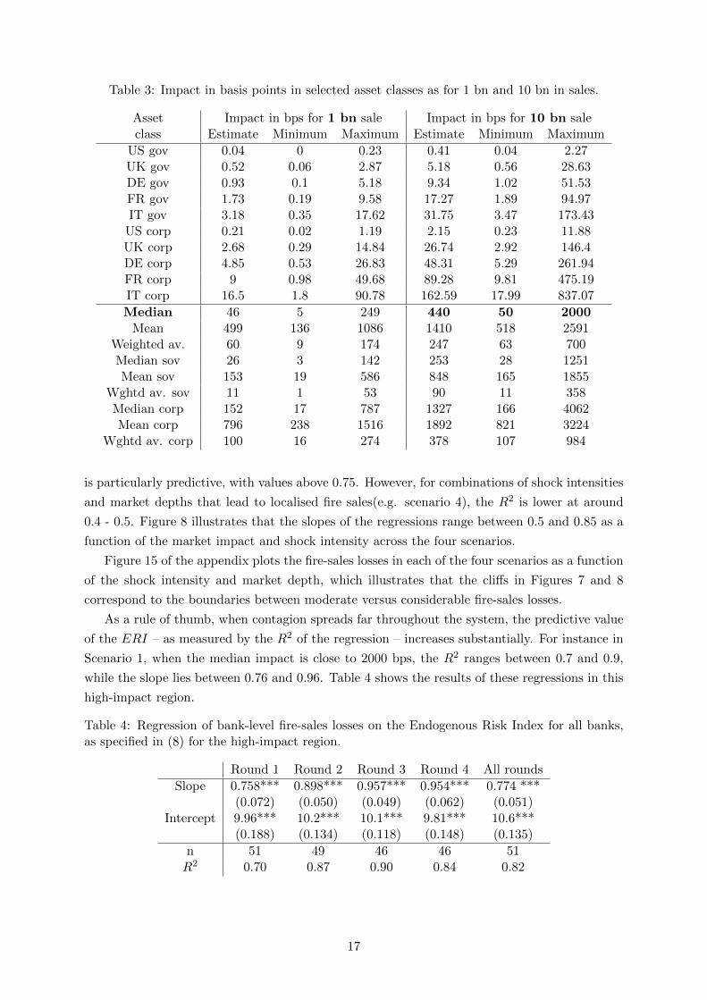
Table 3: Impact in basis points in selected asset classes as for 1 bn and 10 bn in sales.

Asset Impact in bps for 1 bn sale Impact in bps for 10 bn saleclass Estimate Minimum Maximum Estimate Minimum Maximum

US gov 0.04 0 0.23 0.41 0.04 2.27UK gov 0.52 0.06 2.87 5.18 0.56 28.63DE gov 0.93 0.1 5.18 9.34 1.02 51.53FR gov 1.73 0.19 9.58 17.27 1.89 94.97IT gov 3.18 0.35 17.62 31.75 3.47 173.43

US corp 0.21 0.02 1.19 2.15 0.23 11.88UK corp 2.68 0.29 14.84 26.74 2.92 146.4DE corp 4.85 0.53 26.83 48.31 5.29 261.94FR corp 9 0.98 49.68 89.28 9.81 475.19IT corp 16.5 1.8 90.78 162.59 17.99 837.07

Median 46 5 249 440 50 2000Mean 499 136 1086 1410 518 2591

Weighted av. 60 9 174 247 63 700Median sov 26 3 142 253 28 1251Mean sov 153 19 586 848 165 1855

Wghtd av. sov 11 1 53 90 11 358Median corp 152 17 787 1327 166 4062Mean corp 796 238 1516 1892 821 3224

Wghtd av. corp 100 16 274 378 107 984

is particularly predictive, with values above 0.75. However, for combinations of shock intensities

and market depths that lead to localised fire sales(e.g. scenario 4), the R2 is lower at around

0.4 - 0.5. Figure 8 illustrates that the slopes of the regressions range between 0.5 and 0.85 as a

function of the market impact and shock intensity across the four scenarios.

Figure 15 of the appendix plots the fire-sales losses in each of the four scenarios as a function

of the shock intensity and market depth, which illustrates that the cliffs in Figures 7 and 8

correspond to the boundaries between moderate versus considerable fire-sales losses.

As a rule of thumb, when contagion spreads far throughout the system, the predictive value

of the ERI – as measured by the R2 of the regression – increases substantially. For instance in

Scenario 1, when the median impact is close to 2000 bps, the R2 ranges between 0.7 and 0.9,

while the slope lies between 0.76 and 0.96. Table 4 shows the results of these regressions in this

high-impact region.

Table 4: Regression of bank-level fire-sales losses on the Endogenous Risk Index for all banks,as specified in (8) for the high-impact region.

Round 1 Round 2 Round 3 Round 4 All rounds

Slope 0.758*** 0.898*** 0.957*** 0.954*** 0.774 ***(0.072) (0.050) (0.049) (0.062) (0.051)

Intercept 9.96*** 10.2*** 10.1*** 9.81*** 10.6***(0.188) (0.134) (0.118) (0.148) (0.135)

n 51 49 46 46 51R2 0.70 0.87 0.90 0.84 0.82

17

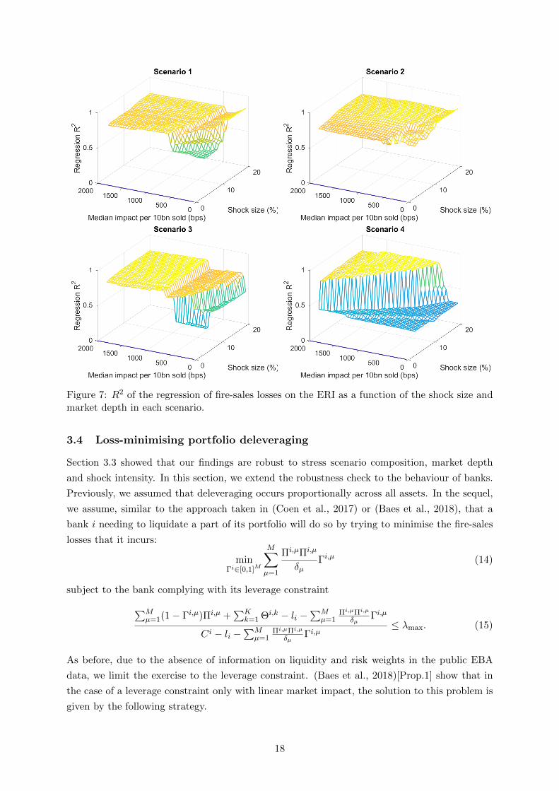
Figure 7: R2 of the regression of fire-sales losses on the ERI as a function of the shock size andmarket depth in each scenario.

3.4 Loss-minimising portfolio deleveraging

Section 3.3 showed that our findings are robust to stress scenario composition, market depth

and shock intensity. In this section, we extend the robustness check to the behaviour of banks.

Previously, we assumed that deleveraging occurs proportionally across all assets. In the sequel,

we assume, similar to the approach taken in (Coen et al., 2017) or (Baes et al., 2018), that a

bank i needing to liquidate a part of its portfolio will do so by trying to minimise the fire-sales

losses that it incurs:

minΓi∈[0,1]M

M∑µ=1

Πi,µΠi,µ

δµΓi,µ (14)

subject to the bank complying with its leverage constraint∑Mµ=1(1− Γi,µ)Πi,µ +

∑Kk=1 Θi,k − li −

∑Mµ=1

Πi,µΠi,µ

δµΓi,µ

Ci − li −∑M

µ=1Πi,µΠi,µ

δµΓi,µ

≤ λmax. (15)

As before, due to the absence of information on liquidity and risk weights in the public EBA

data, we limit the exercise to the leverage constraint. (Baes et al., 2018)[Prop.1] show that in

the case of a leverage constraint only with linear market impact, the solution to this problem is

given by the following strategy.

18

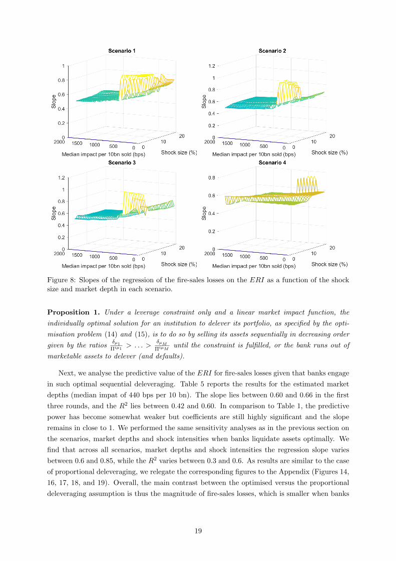
Figure 8: Slopes of the regression of the fire-sales losses on the ERI as a function of the shocksize and market depth in each scenario.

Proposition 1. Under a leverage constraint only and a linear market impact function, the

individually optimal solution for an institution to delever its portfolio, as specified by the opti-

misation problem (14) and (15), is to do so by selling its assets sequentially in decreasing order

given by the ratiosδµ1

Πiµ1> . . . >

δµMΠiµM

until the constraint is fulfilled, or the bank runs out of

marketable assets to delever (and defaults).

Next, we analyse the predictive value of the ERI for fire-sales losses given that banks engage

in such optimal sequential deleveraging. Table 5 reports the results for the estimated market

depths (median impat of 440 bps per 10 bn). The slope lies between 0.60 and 0.66 in the first

three rounds, and the R2 lies between 0.42 and 0.60. In comparison to Table 1, the predictive

power has become somewhat weaker but coefficients are still highly significant and the slope

remains in close to 1. We performed the same sensitivity analyses as in the previous section on

the scenarios, market depths and shock intensities when banks liquidate assets optimally. We

find that across all scenarios, market depths and shock intensities the regression slope varies

between 0.6 and 0.85, while the R2 varies between 0.3 and 0.6. As results are similar to the case

of proportional deleveraging, we relegate the corresponding figures to the Appendix (Figures 14,

16, 17, 18, and 19). Overall, the main contrast between the optimised versus the proportional

deleveraging assumption is thus the magnitude of fire-sales losses, which is smaller when banks

19

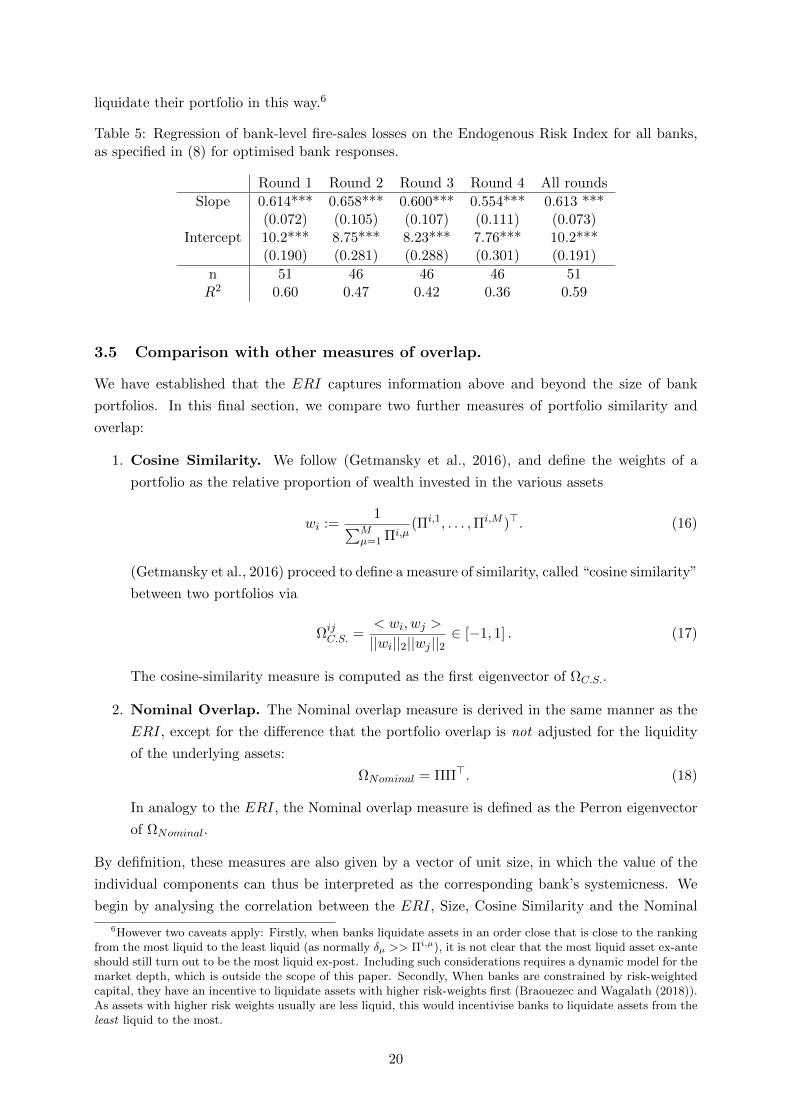
liquidate their portfolio in this way.6

Table 5: Regression of bank-level fire-sales losses on the Endogenous Risk Index for all banks,as specified in (8) for optimised bank responses.

Round 1 Round 2 Round 3 Round 4 All rounds

Slope 0.614*** 0.658*** 0.600*** 0.554*** 0.613 ***(0.072) (0.105) (0.107) (0.111) (0.073)

Intercept 10.2*** 8.75*** 8.23*** 7.76*** 10.2***(0.190) (0.281) (0.288) (0.301) (0.191)

n 51 46 46 46 51R2 0.60 0.47 0.42 0.36 0.59

3.5 Comparison with other measures of overlap.

We have established that the ERI captures information above and beyond the size of bank

portfolios. In this final section, we compare two further measures of portfolio similarity and

overlap:

1. Cosine Similarity. We follow (Getmansky et al., 2016), and define the weights of a

portfolio as the relative proportion of wealth invested in the various assets

wi :=1∑M

µ=1 Πi,µ(Πi,1, . . . ,Πi,M )>. (16)

(Getmansky et al., 2016) proceed to define a measure of similarity, called “cosine similarity”

between two portfolios via

ΩijC.S. =

< wi, wj >

||wi||2||wj ||2∈ [−1, 1] . (17)

The cosine-similarity measure is computed as the first eigenvector of ΩC.S..

2. Nominal Overlap. The Nominal overlap measure is derived in the same manner as the

ERI, except for the difference that the portfolio overlap is not adjusted for the liquidity

of the underlying assets:

ΩNominal = ΠΠ>. (18)

In analogy to the ERI, the Nominal overlap measure is defined as the Perron eigenvector

of ΩNominal.

By defifnition, these measures are also given by a vector of unit size, in which the value of the

individual components can thus be interpreted as the corresponding bank’s systemicness. We

begin by analysing the correlation between the ERI, Size, Cosine Similarity and the Nominal

6However two caveats apply: Firstly, when banks liquidate assets in an order close that is close to the rankingfrom the most liquid to the least liquid (as normally δµ >> Πi,µ), it is not clear that the most liquid asset ex-anteshould still turn out to be the most liquid ex-post. Including such considerations requires a dynamic model for themarket depth, which is outside the scope of this paper. Secondly, When banks are constrained by risk-weightedcapital, they have an incentive to liquidate assets with higher risk-weights first (Braouezec and Wagalath (2018)).As assets with higher risk weights usually are less liquid, this would incentivise banks to liquidate assets from theleast liquid to the most.

20

ERI Nom. Ov. Cos. Sim. Size

ERI 1 0.68 (0.85) -0.13 (- 0.22) 0.60 (0.80)Nom. Ov. 1 -0.14 (-0.22) 0.78 (0.92)Cos. Sim. 1 -0.17 (-0.27)

Size 1

Table 6: Similarity between the various overlap measures: The bold numbers are rank-correlations (Kendall’s τ), while the numbers in brackets are linear correlations (Spearman’sρ).

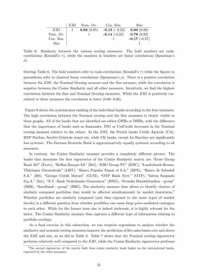
Overlap Table 6. The bold numbers refer to rank-correlations (Kendall’s τ) while the figures in

parentheses refer to classical linear correlations (Spearman’s ρ). There is a positive correlation

between the ERI, the Nominal Overlap measure and the Size measure, while the correlation is

negative between the Cosine Similarity and all other measures. Intuitively, we find the highest

correlation between the Size and Nominal Overlap measures. While the ERI is positively cor-

related to these measures the correlation is lower (0.60- 0.68).

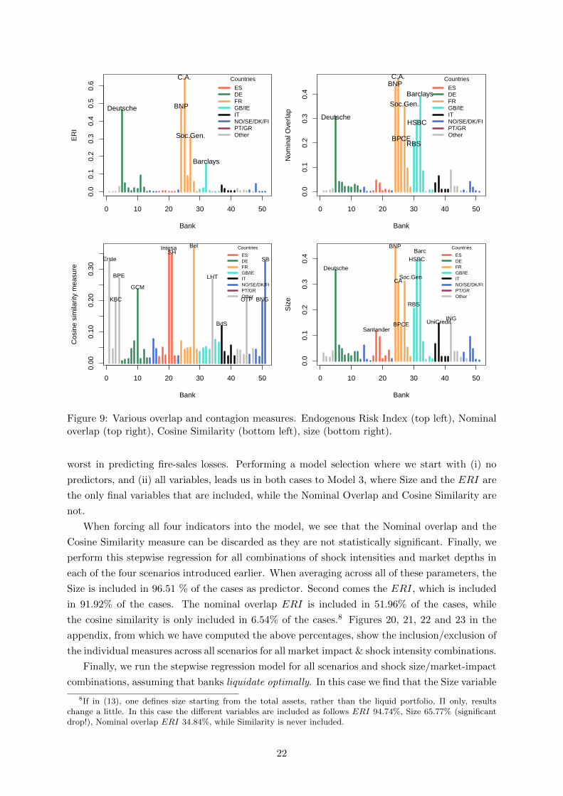
Figure 9 shows the systemicness ranking of the individual banks according to the four measures.

The high correlation between the Nominal overlap and the Size measures is clearly visible in

these graphs. All of the banks that are identified are either GSIBs or DSIBs, with the difference

that the importance of banks such as Santander, ING or UniCredit decreases in the Nominal

overlap measure relative to the others. In the ERI, the French banks Credit Agricole (CA),

BNP Paribas, Societe Generale stand out, while UK banks, except for Barclays are significantly

less systemic. The German Deutsche Bank is approximatively equally systemic according to all

measures.

In contrast, the Cosine Similarity measure provides a completely different picture: The

banks that dominate the first eigenvector of the Cosine Similarity matrix are “Erste Group

Bank AG” (Erste), “Belfius Banque SA” (Bel), “KBC Group NV” (KBC), “Landesbank Hessen-

Thuringen Girozentrale” (LHT), “Banco Popular Espan ol S.A.” (BPE), “Banco de Sabadell

S.A.” (BS), “Groupe Credit Mutuel” (GCM), “OTP Bank Nyrt.” (OTP), “Intesa Sanpaolo

S.p.A.” (Int), “N.V. Bank Nederlandse Gemeenten” (BNG), “Svenska Handelsbanken - group”

(SHB), “Swedbank - group” (SBG). The similarity measure thus allows to identify clusters of

similarly composed portfolios that would be affected simultaneously by market downturns.7

Whether portfolios are similarly composed (and thus exposed to the same types of market

shocks) is a different question from whether portfolios can cause large price-mediated contagion

to each other. While for the former issue size is indeed irrelevant, it is highly relevant for the

latter. The Cosine Similarity measure thus captures a different type of information relating to

portfolio overlaps.

As a final exercise in this subsection, we run stepwise regressions to analyse whether the

similarity and nominal overlap measures improve the prediction of fire-sales losses over and above

the ERI and size, as we did in Table 2. Table 7 shows that the Nominal overlap eigenvector

performs relatively well compared to the ERI, while the Cosine Similarity eigenvector performs

7The second eigenvector of the matrix built from cosine similarity loads higher on the international banks,captured by the other measures.

21

0 10 20 30 40 50

0.0

0.1

0.2

0.3

0.4

0.5

0.6

Bank

ER

I

Deutsche BNP

C.A.

Soc.Gen.

Barclays

Countries

ESDEFRGB/IEITNO/SE/DK/FIPT/GROther

0 10 20 30 40 50

0.0

0.1

0.2

0.3

0.4

Bank

Nom

inal

Ove

rlap

Deutsche

BNPC.A.

BPCE

Soc.Gen.

RBS

HSBC

Barclays

Countries

ESDEFRGB/IEITNO/SE/DK/FIPT/GROther

0 10 20 30 40 50

0.00

0.10

0.20

0.30

Bank

Cos

ine

sim

ilarit

y m

easu

re

Erste

KBC

BPE

GCM

IntesaSH

Bel

LHT

BdS

OTP BNG

SB

Countries

ESDEFRGB/IEITNO/SE/DK/FIPT/GROther

0 10 20 30 40 50

0.0

0.1

0.2

0.3

0.4

Bank

Siz

e

Deutsche

Santander

BNP

CA

BPCE

Soc.Gen

RBS

HSBCBarc

UniCreditING

Countries

ESDEFRGB/IEITNO/SE/DK/FIPT/GROther

Figure 9: Various overlap and contagion measures. Endogenous Risk Index (top left), Nominaloverlap (top right), Cosine Similarity (bottom left), size (bottom right).

worst in predicting fire-sales losses. Performing a model selection where we start with (i) no

predictors, and (ii) all variables, leads us in both cases to Model 3, where Size and the ERI are

the only final variables that are included, while the Nominal Overlap and Cosine Similarity are

not.

When forcing all four indicators into the model, we see that the Nominal overlap and the

Cosine Similarity measure can be discarded as they are not statistically significant. Finally, we

perform this stepwise regression for all combinations of shock intensities and market depths in

each of the four scenarios introduced earlier. When averaging across all of these parameters, the

Size is included in 96.51 % of the cases as predictor. Second comes the ERI, which is included

in 91.92% of the cases. The nominal overlap ERI is included in 51.96% of the cases, while

the cosine similarity is only included in 6.54% of the cases.8 Figures 20, 21, 22 and 23 in the

appendix, from which we have computed the above percentages, show the inclusion/exclusion of

the individual measures across all scenarios for all market impact & shock intensity combinations.

Finally, we run the stepwise regression model for all scenarios and shock size/market-impact

combinations, assuming that banks liquidate optimally. In this case we find that the Size variable

8If in (13), one defines size starting from the total assets, rather than the liquid portfolio, Π only, resultschange a little. In this case the different variables are included as follows ERI 94.74%, Size 65.77% (significantdrop!), Nominal overlap ERI 34.84%, while Similarity is never included.

22

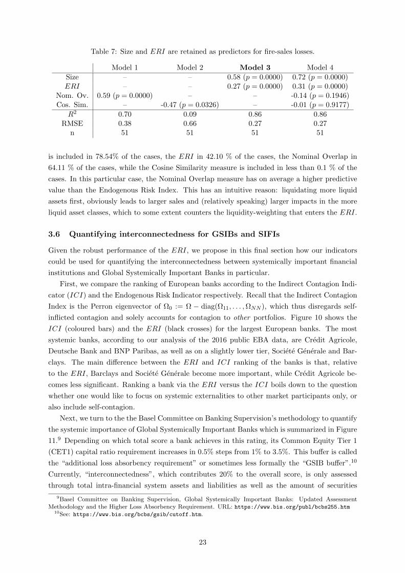
Table 7: Size and ERI are retained as predictors for fire-sales losses.

Model 1 Model 2 Model 3 Model 4

Size – – 0.58 (p = 0.0000) 0.72 (p = 0.0000)ERI – – 0.27 (p = 0.0000) 0.31 (p = 0.0000)

Nom. Ov. 0.59 (p = 0.0000) – – -0.14 (p = 0.1946)Cos. Sim. – -0.47 (p = 0.0326) – -0.01 (p = 0.9177)

R2 0.70 0.09 0.86 0.86RMSE 0.38 0.66 0.27 0.27

n 51 51 51 51

is included in 78.54% of the cases, the ERI in 42.10 % of the cases, the Nominal Overlap in

64.11 % of the cases, while the Cosine Similarity measure is included in less than 0.1 % of the

cases. In this particular case, the Nominal Overlap measure has on average a higher predictive

value than the Endogenous Risk Index. This has an intuitive reason: liquidating more liquid

assets first, obviously leads to larger sales and (relatively speaking) larger impacts in the more

liquid asset classes, which to some extent counters the liquidity-weighting that enters the ERI.

3.6 Quantifying interconnectedness for GSIBs and SIFIs

Given the robust performance of the ERI, we propose in this final section how our indicators

could be used for quantifying the interconnectedness between systemically important financial

institutions and Global Systemically Important Banks in particular.

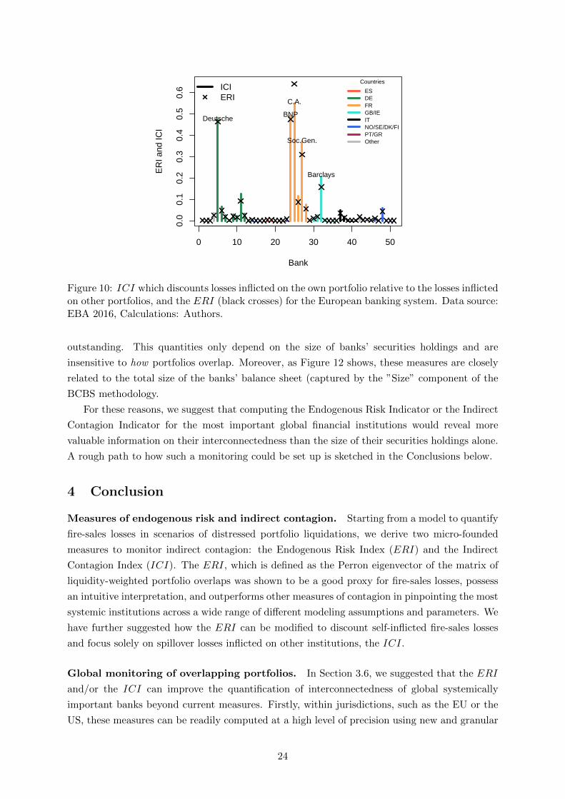
First, we compare the ranking of European banks according to the Indirect Contagion Indi-

cator (ICI) and the Endogenous Risk Indicator respectively. Recall that the Indirect Contagion

Index is the Perron eigenvector of Ω0 := Ω − diag(Ω11, . . . ,ΩNN ), which thus disregards self-

inflicted contagion and solely accounts for contagion to other portfolios. Figure 10 shows the

ICI (coloured bars) and the ERI (black crosses) for the largest European banks. The most

systemic banks, according to our analysis of the 2016 public EBA data, are Credit Agricole,

Deutsche Bank and BNP Paribas, as well as on a slightly lower tier, Societe Generale and Bar-

clays. The main difference between the ERI and ICI ranking of the banks is that, relative

to the ERI, Barclays and Societe Generale become more important, while Credit Agricole be-

comes less significant. Ranking a bank via the ERI versus the ICI boils down to the question

whether one would like to focus on systemic externalities to other market participants only, or

also include self-contagion.

Next, we turn to the the Basel Committee on Banking Supervision’s methodology to quantify

the systemic importance of Global Systemically Important Banks which is summarized in Figure

11.9 Depending on which total score a bank achieves in this rating, its Common Equity Tier 1

(CET1) capital ratio requirement increases in 0.5% steps from 1% to 3.5%. This buffer is called

the “additional loss absorbency requirement” or sometimes less formally the “GSIB buffer”.10

Currently, “interconnectedness”, which contributes 20% to the overall score, is only assessed

through total intra-financial system assets and liabilities as well as the amount of securities

9Basel Committee on Banking Supervision, Global Systemically Important Banks: Updated AssessmentMethodology and the Higher Loss Absorbency Requirement. URL: https://www.bis.org/publ/bcbs255.htm

10See: https://www.bis.org/bcbs/gsib/cutoff.htm.

23

0 10 20 30 40 50

0.0

0.1

0.2

0.3

0.4

0.5

0.6

Bank

ER

I and

ICI

DeutscheBNP

C.A.

Soc.Gen.

Barclays

Countries

ESDEFRGB/IEITNO/SE/DK/FIPT/GROther

ICIERI

Figure 10: ICI which discounts losses inflicted on the own portfolio relative to the losses inflictedon other portfolios, and the ERI (black crosses) for the European banking system. Data source:EBA 2016, Calculations: Authors.

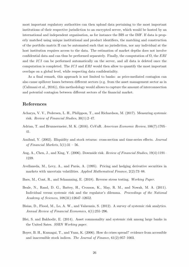
outstanding. This quantities only depend on the size of banks’ securities holdings and are

insensitive to how portfolios overlap. Moreover, as Figure 12 shows, these measures are closely

related to the total size of the banks’ balance sheet (captured by the ”Size” component of the

BCBS methodology.

For these reasons, we suggest that computing the Endogenous Risk Indicator or the Indirect

Contagion Indicator for the most important global financial institutions would reveal more

valuable information on their interconnectedness than the size of their securities holdings alone.

A rough path to how such a monitoring could be set up is sketched in the Conclusions below.

4 Conclusion

Measures of endogenous risk and indirect contagion. Starting from a model to quantify

fire-sales losses in scenarios of distressed portfolio liquidations, we derive two micro-founded

measures to monitor indirect contagion: the Endogenous Risk Index (ERI) and the Indirect

Contagion Index (ICI). The ERI, which is defined as the Perron eigenvector of the matrix of

liquidity-weighted portfolio overlaps was shown to be a good proxy for fire-sales losses, possess

an intuitive interpretation, and outperforms other measures of contagion in pinpointing the most

systemic institutions across a wide range of different modeling assumptions and parameters. We

have further suggested how the ERI can be modified to discount self-inflicted fire-sales losses

and focus solely on spillover losses inflicted on other institutions, the ICI.

Global monitoring of overlapping portfolios. In Section 3.6, we suggested that the ERI

and/or the ICI can improve the quantification of interconnectedness of global systemically

important banks beyond current measures. Firstly, within jurisdictions, such as the EU or the

US, these measures can be readily computed at a high level of precision using new and granular

24

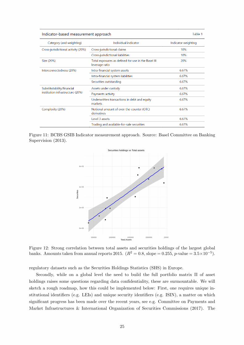
Figure 11: BCBS GSIB Indicator measurement approach. Source: Basel Committee on BankingSupervision (2013).

0e+00

2e+05

4e+05

6e+05

500000 1000000 1500000 2000000 2500000

Total.Assets

Sec

uriti

es

Securities holdings vs Total assets

Figure 12: Strong correlation between total assets and securities holdings of the largest globalbanks. Amounts taken from annual reports 2015. (R2 = 0.8, slope = 0.255, p-value = 3.5×10−5).

regulatory datasets such as the Securities Holdings Statistics (SHS) in Europe.

Secondly, while on a global level the need to build the full portfolio matrix Π of asset

holdings raises some questions regarding data confidentiality, these are surmountable. We will

sketch a rough roadmap, how this could be implemented below: First, one requires unique in-

stitutional identifiers (e.g. LEIs) and unique security identifiers (e.g. ISIN), a matter on which

significant progress has been made over the recent years, see e.g. Committee on Payments and

Market Infrastructures & International Organization of Securities Commissions (2017). The

25

most important regulatory authorities can then upload data pertaining to the most important

institutions of their respective jurisdiction to an encrypted server, which would be hosted by an

international and independent organisation, as for instance the BIS or the IMF. If data is prop-

erly matched using unique institutional and product identifiers, the matching and construction

of the portfolio matrix Π can be automated such that no jurisdiction, nor any individual at the

host institution requires access to the data. The estimation of market depths does not involve

confidential data and can thus be performed separately. Finally, the computation of Ω, the ERI

and the ICI can be performed automatically on the server, and all data is deleted once the

computation is completed. The ICI and ERI would then allow to quantify the most important

overlaps on a global level, while respecting data confidentiality.

As a final remark, this approach is not limited to banks: as price-mediated contagion can

also cause spillover losses between different sectors (e.g. from the asset management sector as in

(Calimani et al., 2016)), this methodology would allows to capture the amount of interconnection

and potential contagion between different sectors of the financial market.

References

Acharya, V. V., Pedersen, L. H., Philippon, T., and Richardson, M. (2017). Measuring systemic

risk. Review of Financial Studies, 30(1):2–47.

Adrian, T. and Brunnermeier, M. K. (2016). CoVaR. American Economic Review, 106(7):1705–

41.

Amihud, Y. (2002). Illiquidity and stock returns: cross-section and time-series effects. Journal

of Financial Markets, 5(1):31 – 56.

Ang, A., Chen, J., and Xing, Y. (2006). Downside risk. Review of Financial Studies, 19(4):1191–

1239.

Avellaneda, M., Levy, A., and Paras, A. (1995). Pricing and hedging derivative securities in

markets with uncertain volatilities. Applied Mathematical Finance, 2(2):73–88.

Baes, M., Cont, R., and Schaanning, E. (2018). Reverse stress testing. Working Paper.

Beale, N., Rand, D. G., Battey, H., Croxson, K., May, R. M., and Nowak, M. A. (2011).

Individual versus systemic risk and the regulator’s dilemma. Proceedings of the National

Academy of Sciences, 108(31):12647–12652.

Bisias, D., Flood, M., Lo, A. W., and Valavanis, S. (2012). A survey of systemic risk analytics.

Annual Review of Financial Economics, 4(1):255–296.

Blei, S. and Bakhodir, E. (2014). Asset commonality and systemic risk among large banks in

the United Sates. SSRN Working paper.

Boyer, B. H., Kumagai, T., and Yuan, K. (2006). How do crises spread? evidence from accessible

and inaccessible stock indices. The Journal of Finance, 61(2):957–1003.

26

Braouezec, Y. and Wagalath, L. (2018). Risk-based capital requirements and optimal liquidation

in a stress scenario. Review of Finance, 22:747–782.

Braverman, A. and Minca, A. (2016). Networks of common asset holdings: Aggregation and

measures of vulnerability. Statistics and Risk Modeling, Forthcoming.

Brownlees, C. and Engle, R. F. (2016). Srisk: A conditional capital shortfall measure of systemic

risk. Review of Financial Studies.

Caccioli, F., Farmer, J. D., Foti, N., and Rockmore, D. (2015). Overlapping portfolios, contagion,

and financial stability. Journal of Economic Dynamics and Control, 51(0):50 – 63.

Caccioli, F., Shrestha, M., Moore, C., and Farmer, J. D. (2014a). Stability analysis of financial

contagion due to overlapping portfolios. Journal of Banking and Finance, 46:233 – 245.

Caccioli, F., Shrestha, M., Moore, C., and Farmer, J. D. (2014b). Stability analysis of financial

contagion due to overlapping portfolios. Journal of Banking & Finance, 46:233 – 245.

Calimani, S., Halaj, G., and Zochowski, D. (2016). Simulating fire-sales in banking and shadow

banking system. Mimeo.

Coen, J., Lepore, C., and Schaanning, E. (2017). Taking regulation seriously: Fire sales under

solvency and liquidty constraints. Working paper.

Committee on Payments and Market Infrastructures & International Organization of Securities

Commissions (2017). Harmonisation of the unique product identifier. BIS.

Cont, R. and Schaanning, E. (2016). Fire sales, indirect contragion and systemic stress testing.

Norges Bank Working paper.

Cont, R. and Wagalath, L. (2013). Running for the exit: Distressed selling and endogenous

correlation in financial markets. Mathematical Finance, 23:718–741.

Cont, R. and Wagalath, L. (2016). Fire sales forensics: Measuring endogenous risk. Mathematical

Finance, 26:835–866.

Danielsson, J., Shin, H. S., and Zigrand, J.-P. (2012). Procyclical leverage and endogenous risk.

Working Paper.

Duffie, D. (2010). How Big Banks Fail and What to Do About It? Princeton University Press.

Ellul, A., Jotikasthira, C., and Lundblad, C. T. (2011). Regulatory pressure and fire sales in

the corporate bond market. Journal of Financial Economics, 101(3):596 – 620.

Getmansky, M., Girardi, G., Hanley, K. W., Nikolova, S., and Pelizzon, L. (2016). Portfolio

similarity and asset liquidation in the insurance industry. SSRN Working paper.

Granovetter, M. (1978). Threshold models of collective behavior. American Journal of Sociology,

83:489–515.

27

Guo, W., Minca, A., and Wang, L. (2015). The topology of overlapping portfolio networks.

Statistics and Risk Modeling, 33(3-4):139–155.

Ibragimov, R., Jaffee, D., and Walden, J. (2011). Diversification disasters. Journal of Financial

Economics, 99(2):333 – 348.

Jotikasthira, C., Lundblad, C. T., and Ramadorai, T. (2012). Asset fire sales and purchases and

the international transmission of funding shocks. Journal of Finance, 67(6):2015–2050.

Khandani, A. E. and Lo, A. W. (2011). What happened to the quants in august 2007? evidence

from factors and transactions data. Journal of Financial Markets, 14(1):1–46.

Kritzman, M., Li, Y., Page, S., and Rigobon, R. (2011). Principal components as a measure of

systemic risk. The Journal of Portfolio Management, 37(4):112–126.

Kyle, A. and Obizhaeva, A. (2016). Trading liquidity and funding liquidity in fixed income

markets: Implications of market microstructure invariance. Working paper.

Manconi, A., Massa, M., and Yasuda, A. (2012). The role of institutional investors in propagating

the crisis of 2007 - 2008. Journal of Financial Economics, 104(3):491 – 518.

Obizhaeva, A. (2012). Liquidity estimates and selection bias. Working paper.

Pedersen, L. H. (2009). When Everyone Runs for the Exit. The International Journal of Central

Banking, 5:177–199.

Shleifer, A. and Vishny, R. W. (1992). Liquidation values and debt capacity: A market equilib-

rium approach. The Journal of Finance, 47(4):1343–1366.

Timmer, Y. (2016). Cyclical investment behaviour across financial institutions. Journal of

Financial Economics, forthcoming.

Wagner, W. (2011). Systemic liquidation risk and the Diversity – Diversification trade-off. The

Journal of Finance, 66(4):1141–1175.

28

A Appendix

Figure 13: Bank-level fire-sales losses regressed on the ERI under proportional deleveraging.

29

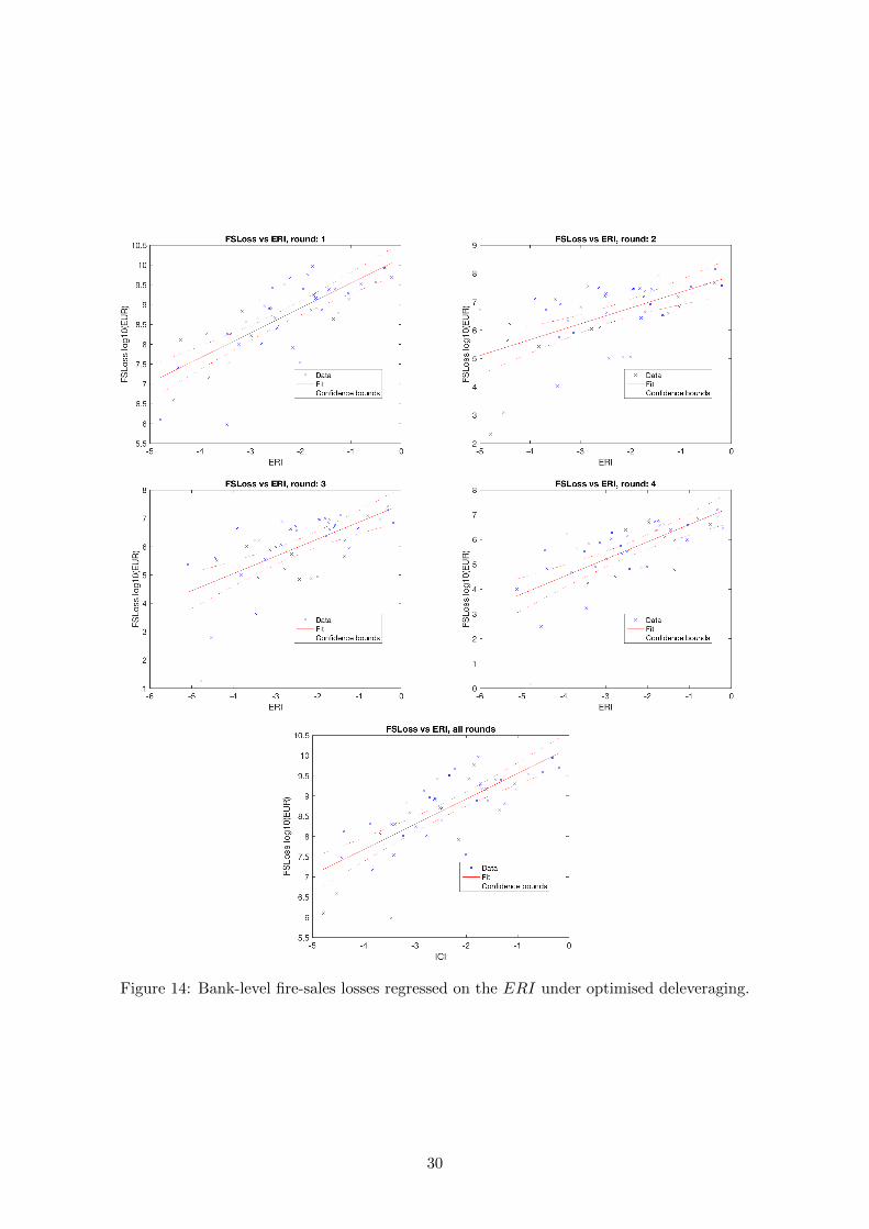
Figure 14: Bank-level fire-sales losses regressed on the ERI under optimised deleveraging.

30

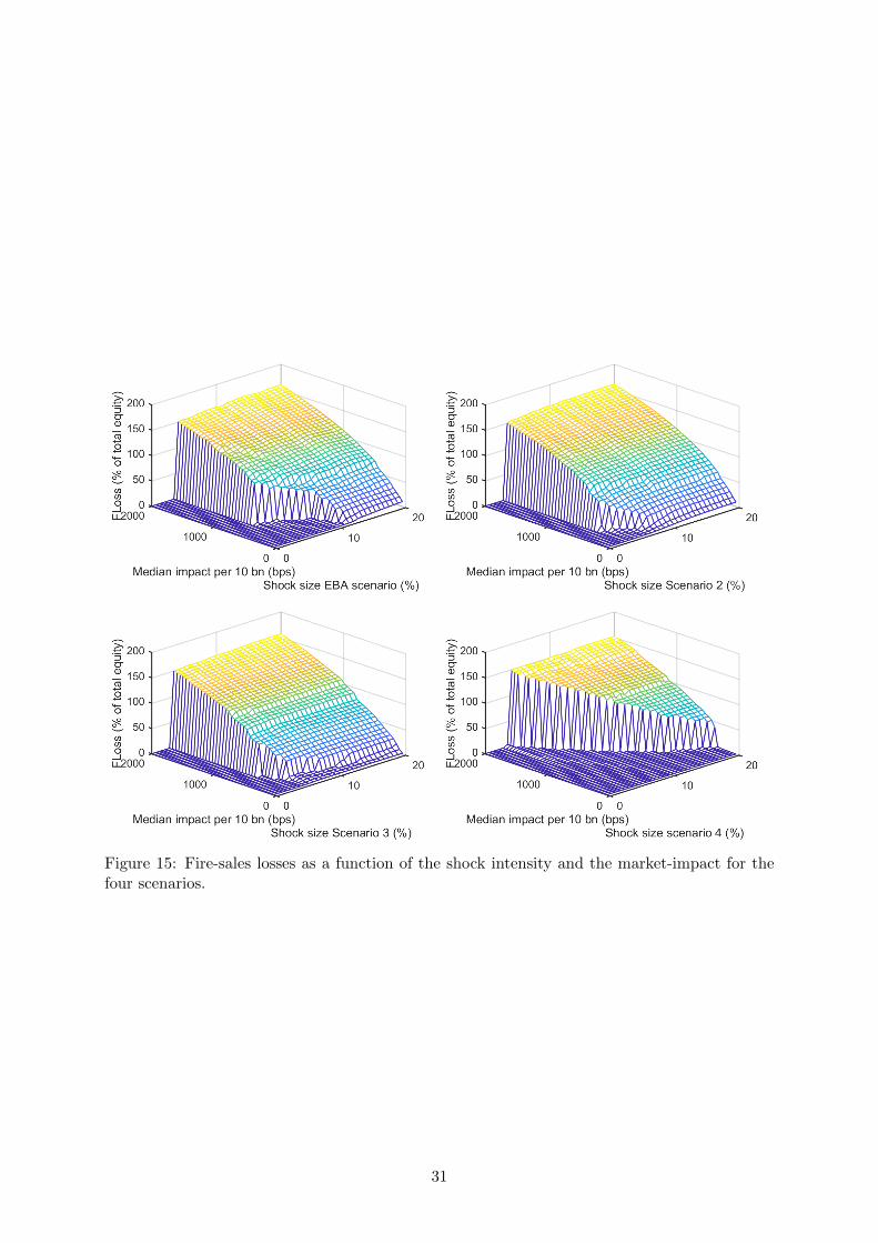
Figure 15: Fire-sales losses as a function of the shock intensity and the market-impact for thefour scenarios.

31

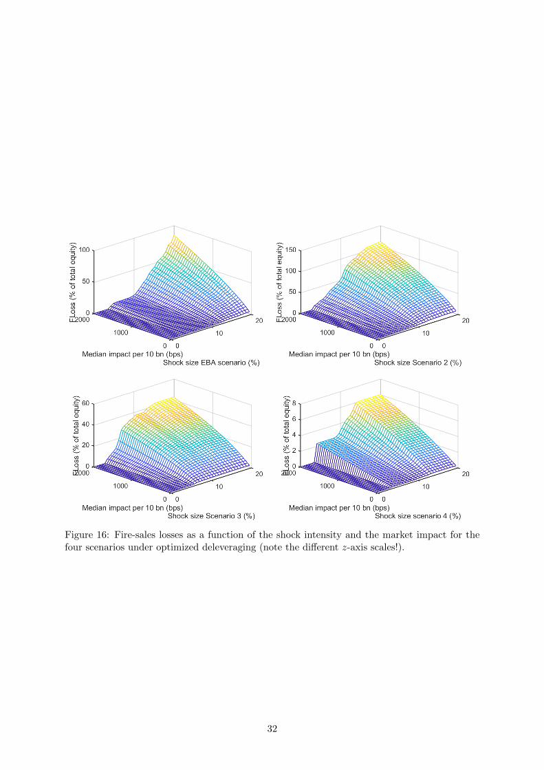
Figure 16: Fire-sales losses as a function of the shock intensity and the market impact for thefour scenarios under optimized deleveraging (note the different z-axis scales!).

32

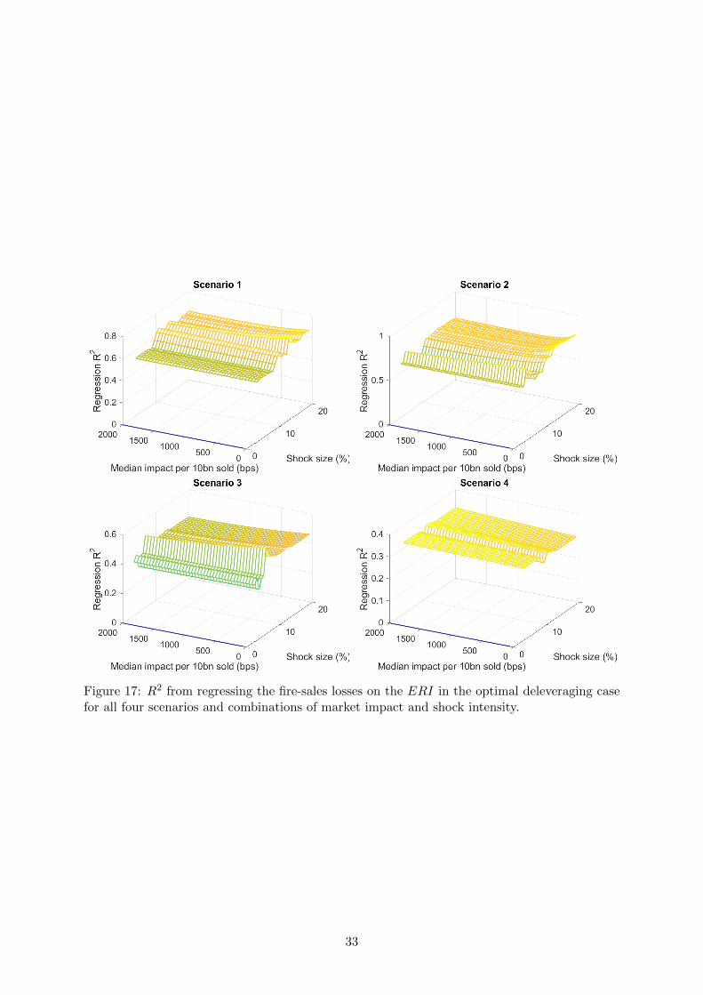
Figure 17: R2 from regressing the fire-sales losses on the ERI in the optimal deleveraging casefor all four scenarios and combinations of market impact and shock intensity.

33

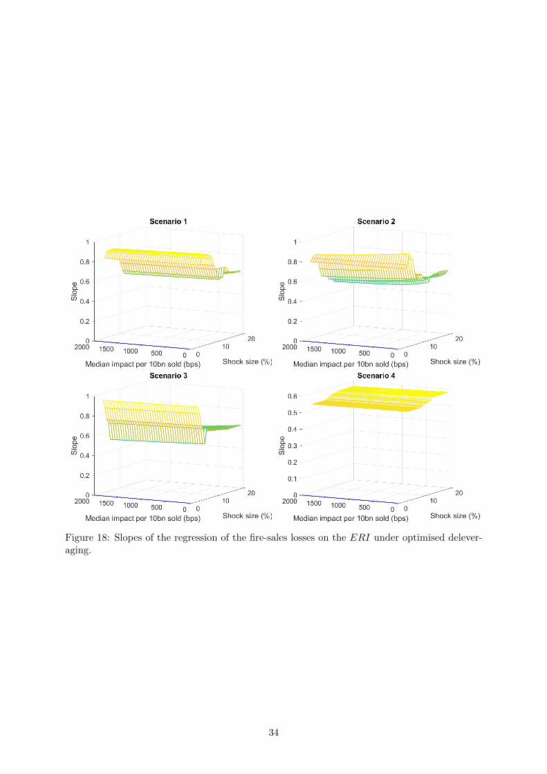
Figure 18: Slopes of the regression of the fire-sales losses on the ERI under optimised delever-aging.

34

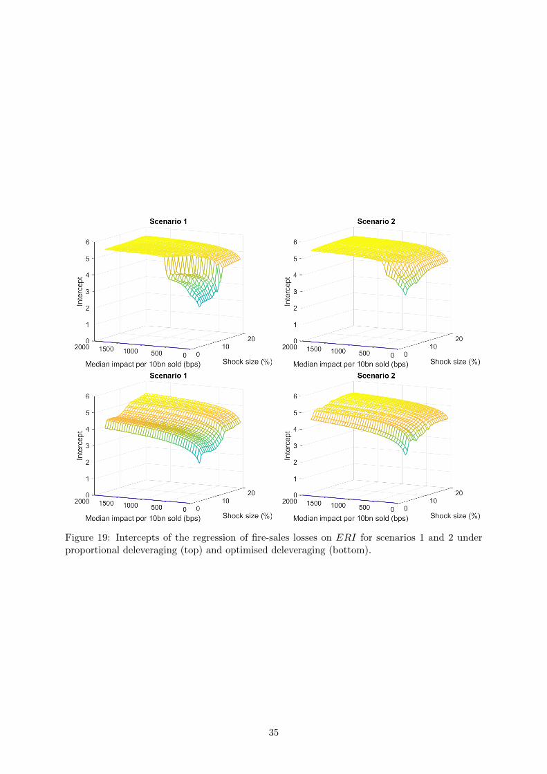
Figure 19: Intercepts of the regression of fire-sales losses on ERI for scenarios 1 and 2 underproportional deleveraging (top) and optimised deleveraging (bottom).

35

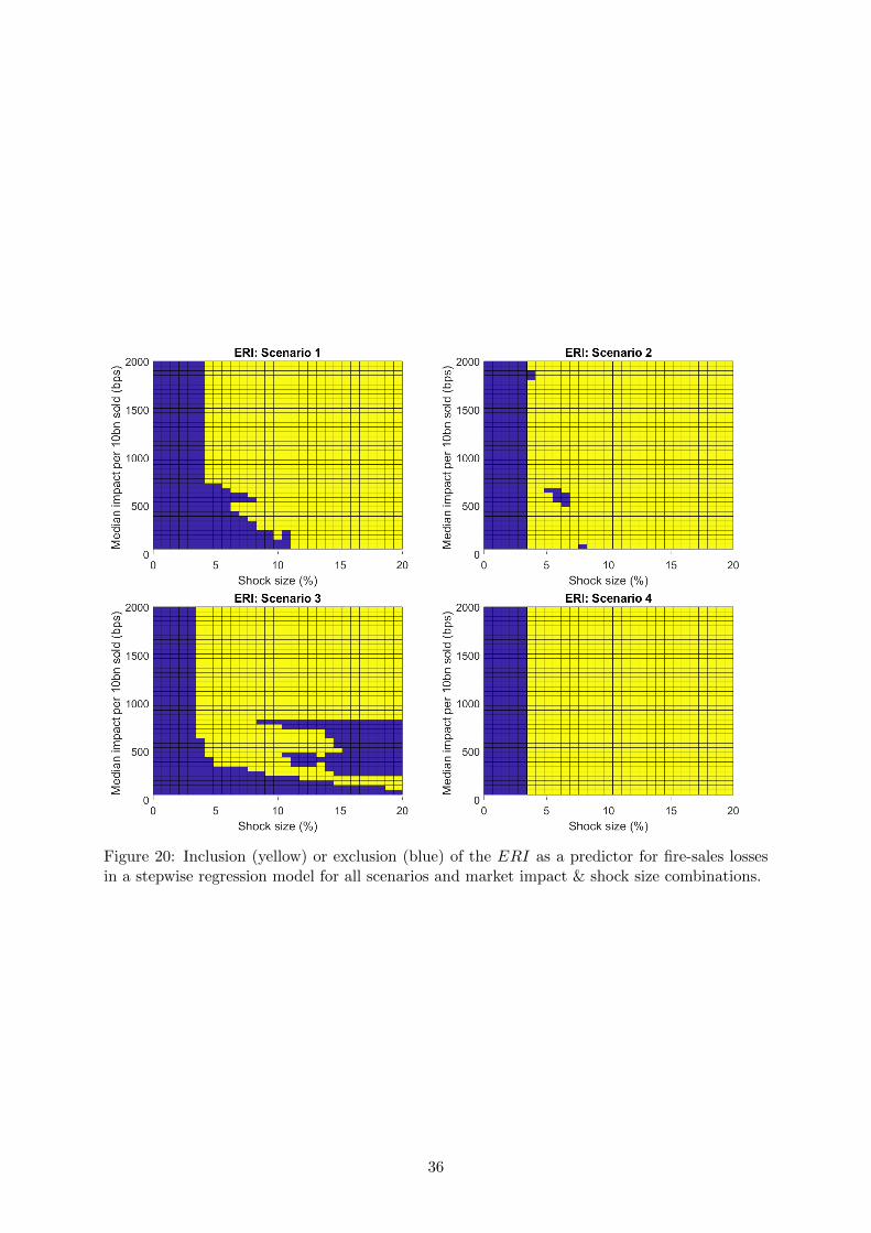
Figure 20: Inclusion (yellow) or exclusion (blue) of the ERI as a predictor for fire-sales lossesin a stepwise regression model for all scenarios and market impact & shock size combinations.

36

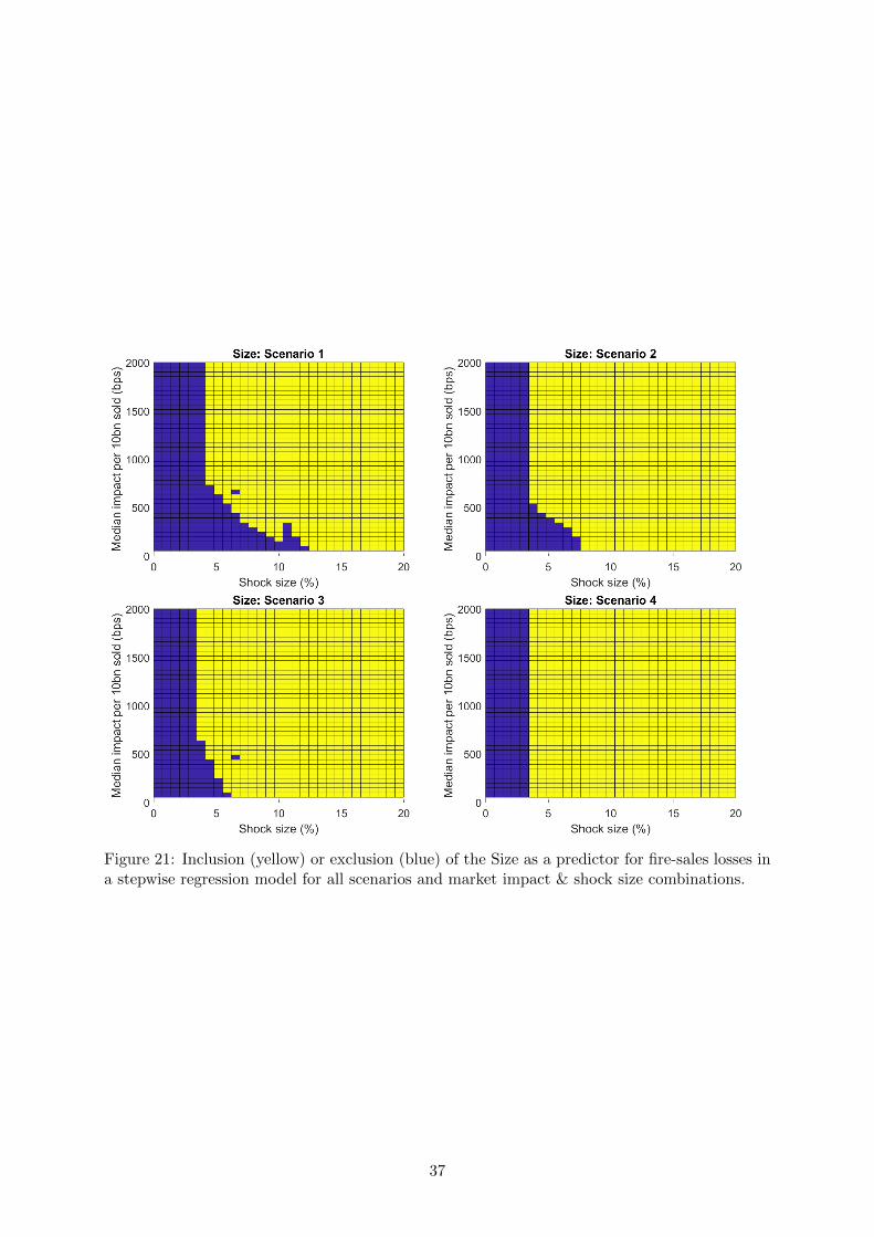
Figure 21: Inclusion (yellow) or exclusion (blue) of the Size as a predictor for fire-sales losses ina stepwise regression model for all scenarios and market impact & shock size combinations.

37

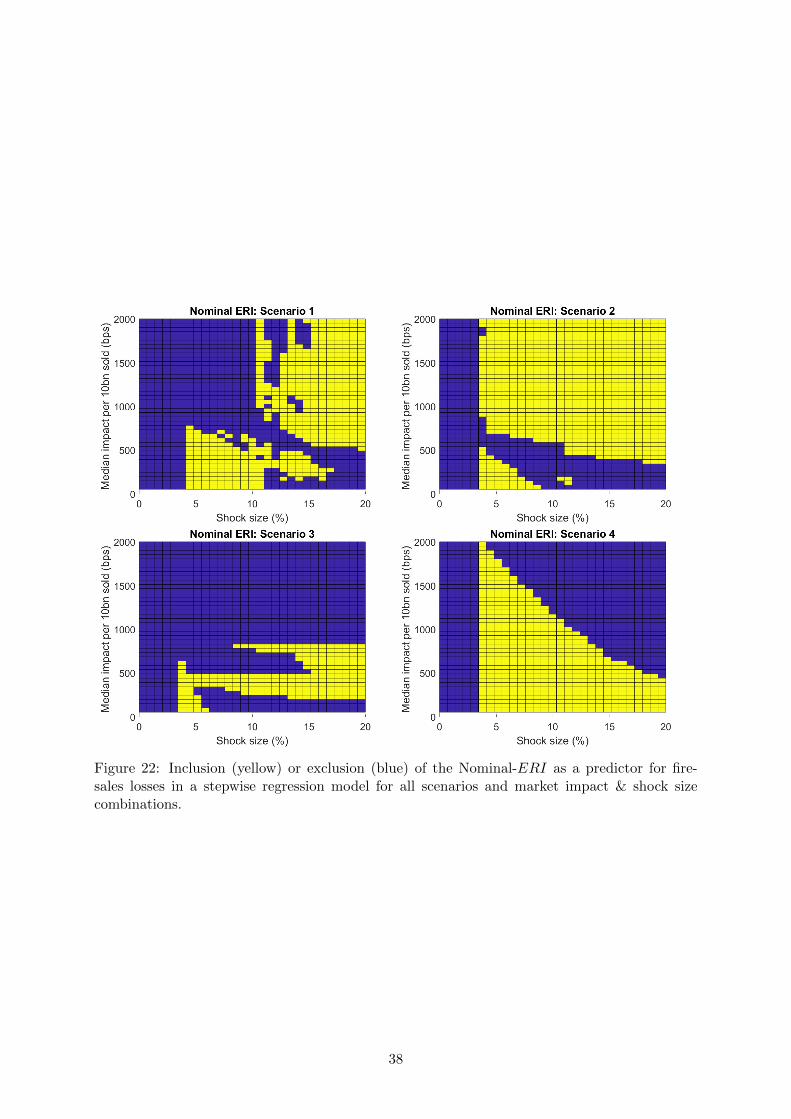
Figure 22: Inclusion (yellow) or exclusion (blue) of the Nominal-ERI as a predictor for fire-sales losses in a stepwise regression model for all scenarios and market impact & shock sizecombinations.

38

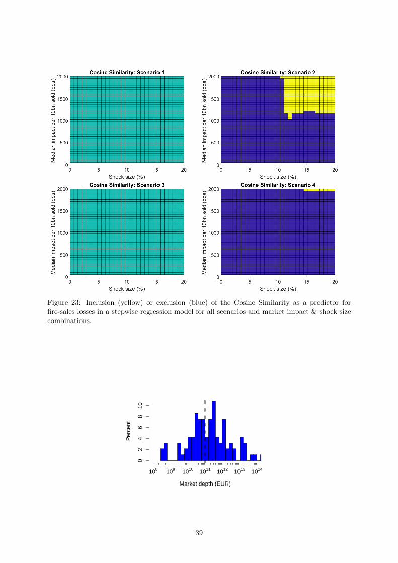
Figure 23: Inclusion (yellow) or exclusion (blue) of the Cosine Similarity as a predictor forfire-sales losses in a stepwise regression model for all scenarios and market impact & shock sizecombinations.

Market depth (EUR)

Per

cent

02

46

810

108 109 1010 1011 1012 1013 1014

39

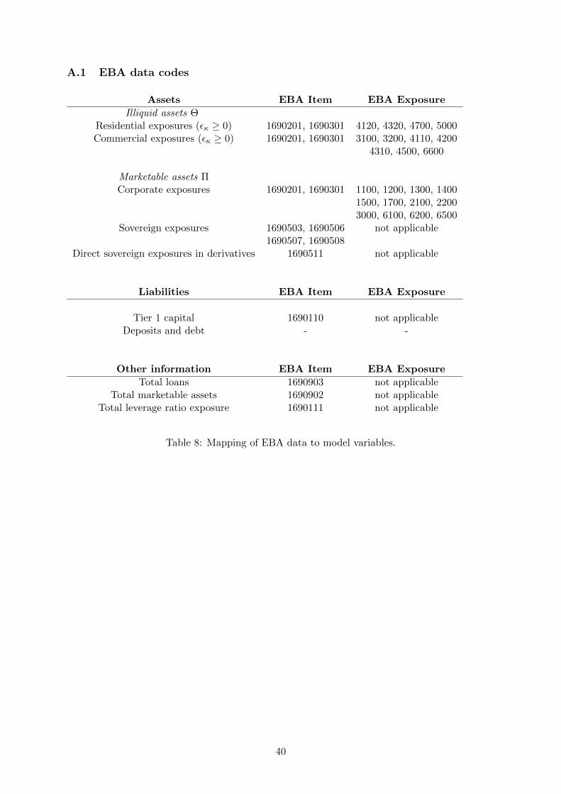
A.1 EBA data codes

Assets EBA Item EBA Exposure

Illiquid assets ΘResidential exposures (εκ ≥ 0) 1690201, 1690301 4120, 4320, 4700, 5000Commercial exposures (εκ ≥ 0) 1690201, 1690301 3100, 3200, 4110, 4200

4310, 4500, 6600

Marketable assets ΠCorporate exposures 1690201, 1690301 1100, 1200, 1300, 1400

1500, 1700, 2100, 22003000, 6100, 6200, 6500

Sovereign exposures 1690503, 1690506 not applicable1690507, 1690508

Direct sovereign exposures in derivatives 1690511 not applicable

Liabilities EBA Item EBA Exposure

Tier 1 capital 1690110 not applicableDeposits and debt - -

Other information EBA Item EBA Exposure

Total loans 1690903 not applicableTotal marketable assets 1690902 not applicable

Total leverage ratio exposure 1690111 not applicable

Table 8: Mapping of EBA data to model variables.

40