Monitoring Bernoulli ProcessesMonitoring Bernoulli Processes

William H. WoodallWilliam H. WoodallVirginia TechVirginia Techbwoodall@vt.edu

OutlineOutline

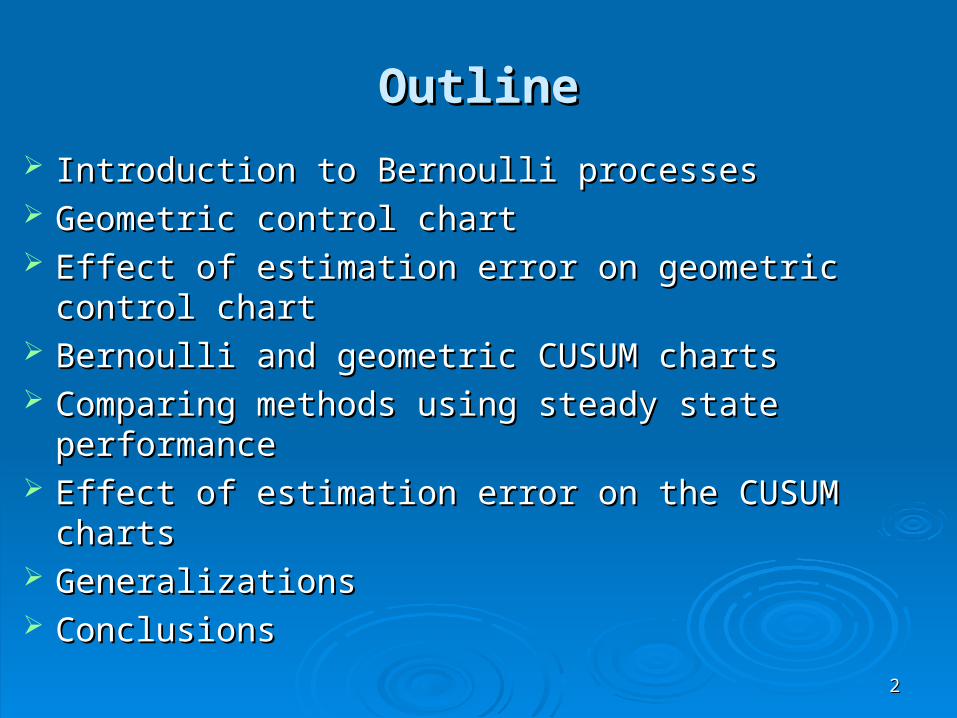
Introduction to Bernoulli processesIntroduction to Bernoulli processes Geometric control chartGeometric control chart Effect of estimation error on geometric control chartEffect of estimation error on geometric control chart Bernoulli and geometric CUSUM chartsBernoulli and geometric CUSUM charts Comparing methods using steady state performanceComparing methods using steady state performance Effect of estimation error on the CUSUM chartsEffect of estimation error on the CUSUM charts GeneralizationsGeneralizations ConclusionsConclusions

22

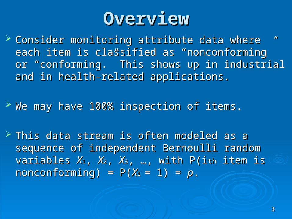
OverviewOverview Consider monitoring attribute data where each item is Consider monitoring attribute data where each item is

classified as “nonconforming” or “conforming.” This classified as “nonconforming” or “conforming.” This shows up in industrial and in health–related shows up in industrial and in health–related applications.applications.

We may have 100% inspection of items.We may have 100% inspection of items.

This data stream is often modeled as a sequence of This data stream is often modeled as a sequence of independent Bernoulli random variables independent Bernoulli random variables XX11, , XX22, , XX33, , …, with P(i…, with P(ithth item is nonconforming) = P( item is nonconforming) = P(XXi i = 1) = = 1) = pp..

33

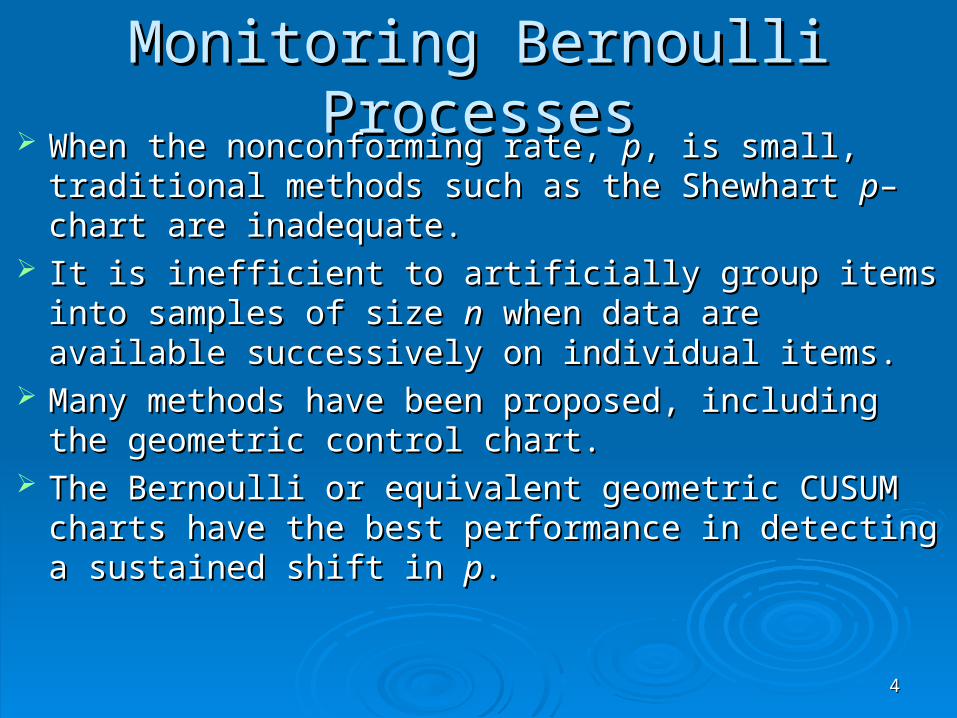
Monitoring Bernoulli ProcessesMonitoring Bernoulli Processes When the nonconforming rate, When the nonconforming rate, pp, is small, traditional , is small, traditional

methods such as the Shewhart methods such as the Shewhart pp–chart are inadequate.–chart are inadequate. It is inefficient to artificially group items into samples of It is inefficient to artificially group items into samples of

size size nn when data are available successively on when data are available successively on individual items. individual items.

Many methods have been proposed, including the Many methods have been proposed, including the geometric control chart.geometric control chart.

The Bernoulli or equivalent geometric CUSUM charts The Bernoulli or equivalent geometric CUSUM charts have the best performance in detecting a sustained have the best performance in detecting a sustained shift in shift in pp..

44

55

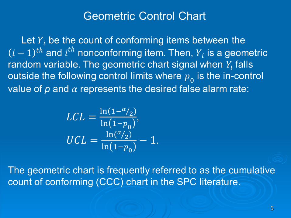
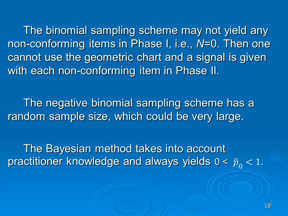
Note that points plotted below the LCL of the Note that points plotted below the LCL of the geometric chart indicate process deterioration, geometric chart indicate process deterioration, whereas points above the UCL indicate process whereas points above the UCL indicate process improvement.improvement.

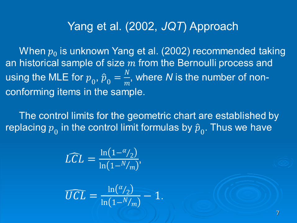
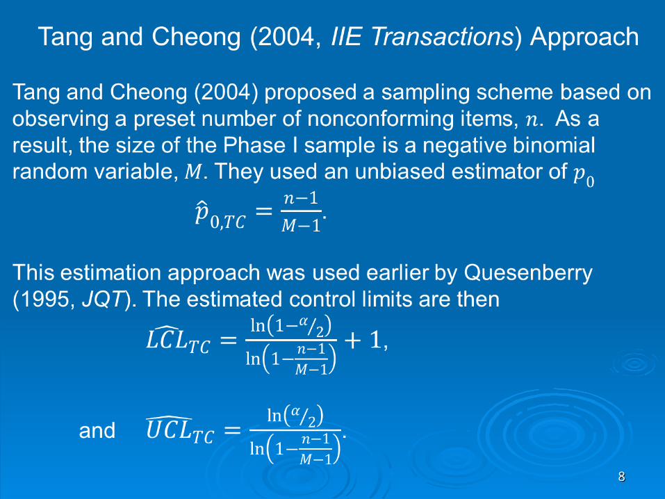
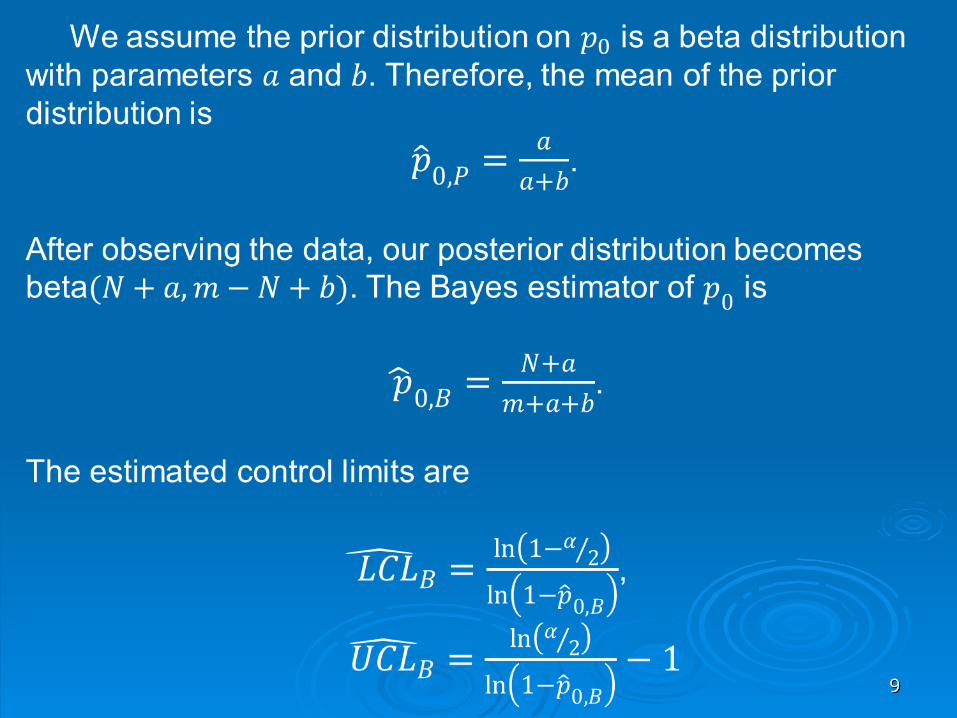
Generally Generally pp00 will be unknown and must be estimated will be unknown and must be estimated using a Phase I sample. Three approaches have been using a Phase I sample. Three approaches have been proposed – binomial sampling, negative binomial proposed – binomial sampling, negative binomial sampling, and the use of a Bayes estimator.sampling, and the use of a Bayes estimator.

66

77

88

99

1010

Performance MetricsPerformance Metrics Charts should be compared based on the average number of Charts should be compared based on the average number of

observations until a signal occurs, the observations until a signal occurs, the ANOSANOS. Charts are designed so . Charts are designed so that the in-control that the in-control ANOSANOS, , ANOSANOS00, is a specified value. , is a specified value.

Equivalently we can consider the average run length (Equivalently we can consider the average run length (ARLARL), the average ), the average number of points plotted until a signal occurs, since number of points plotted until a signal occurs, since ANOSANOS = = ARLARL//pp. .

When When pp00 is estimated, the actual in-control is estimated, the actual in-control ANOSANOS value becomes a value becomes a random variable. We would like the average value to be the specified random variable. We would like the average value to be the specified ANOSANOS00, but we also need the standard deviation of the in-control , but we also need the standard deviation of the in-control ANOSANOS to be low enough that practitioners are confident in getting the desired to be low enough that practitioners are confident in getting the desired value.value.

Previous work on the effect of estimation on the geometric chart has Previous work on the effect of estimation on the geometric chart has considered only the average in-control considered only the average in-control ANOSANOS value, not the standard value, not the standard deviation. deviation.

1111

1212

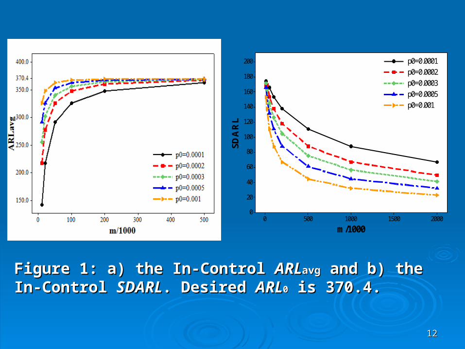
Figure 1: a) the In-Control Figure 1: a) the In-Control ARLARLavgavg and b) the In-Control and b) the In-Control SDARLSDARL. Desired . Desired ARLARL00 is 370.4. is 370.4.

2000150010005000

200

180

160

140

120

100

80

60

40

20

0

m/1000S

DA

RL

p0=0.0001

p0=0.0002

p0=0.0003

p0=0.0005

p0=0.001

The in-control The in-control ARLARLavgavg value converges relatively quickly value converges relatively quickly to the desired value, but the in-control to the desired value, but the in-control SDARL SDARL converges relatively slowly to zero. converges relatively slowly to zero.

This means that for the geometric chart to have reliable This means that for the geometric chart to have reliable and predictable in-control performance, the Phase I and predictable in-control performance, the Phase I sample size must be quite large. sample size must be quite large.

The required sample size can be an order of The required sample size can be an order of magnitude higher than previously recognized.magnitude higher than previously recognized.

1313

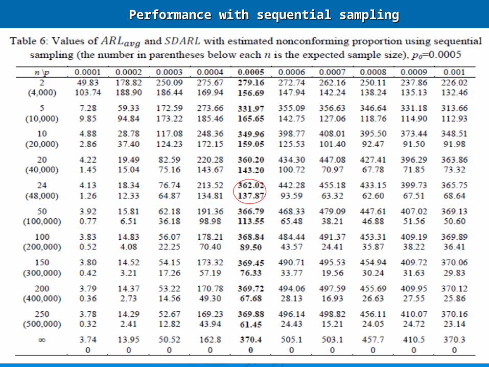
Performance with sequential samplingPerformance with sequential sampling

1515

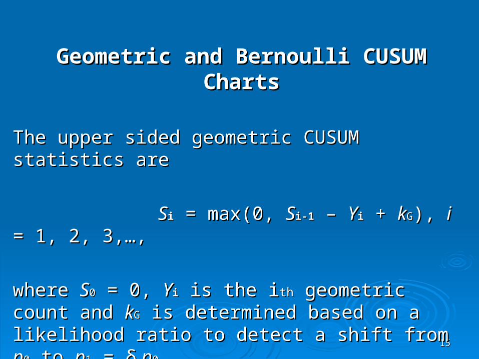
Geometric and Bernoulli CUSUM ChartsGeometric and Bernoulli CUSUM Charts

The upper sided geometric CUSUM statistics areThe upper sided geometric CUSUM statistics are

SSii = max(0, = max(0, SSi-1i-1 – – YYii + + kkGG), ), ii = 1, 2, 3,…, = 1, 2, 3,…,

where where SS00 = 0, = 0, YYii is the i is the ithth geometric count and geometric count and kkGG is is determined based on a likelihood ratio to detect a shift determined based on a likelihood ratio to detect a shift from from pp00 to to pp11 = = δδ p p00. .

A signal is given when A signal is given when SSi i > > hhGG..

1616

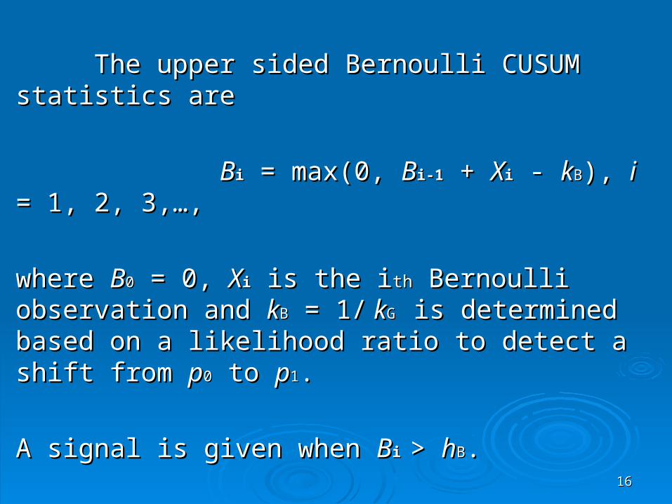
The upper sided Bernoulli CUSUM statistics areThe upper sided Bernoulli CUSUM statistics are

BBii = max(0, = max(0, BBi-1i-1 + + XXii - - kkBB), ), ii = 1, 2, 3,…, = 1, 2, 3,…,

where where BB00 = 0, = 0, XXii is the i is the ithth Bernoulli observation and Bernoulli observation and kkBB = = 1/1/ k kG G is determined based on a likelihood ratio to detect is determined based on a likelihood ratio to detect a shift from a shift from pp00 to to pp11. .

A signal is given when A signal is given when BBi i > > hhBB..

The geometric and Bernoulli CUSUM charts are The geometric and Bernoulli CUSUM charts are equivalentequivalent if if BB00 = 1 – = 1 – kkBB and and hhB B = ( = (hhG G + + kkB B – 1) / – 1) / kkGG..

1717

0 10 20 30 40 50

0.0

0.5

1.0

1.5

2.0

2.5

3.0

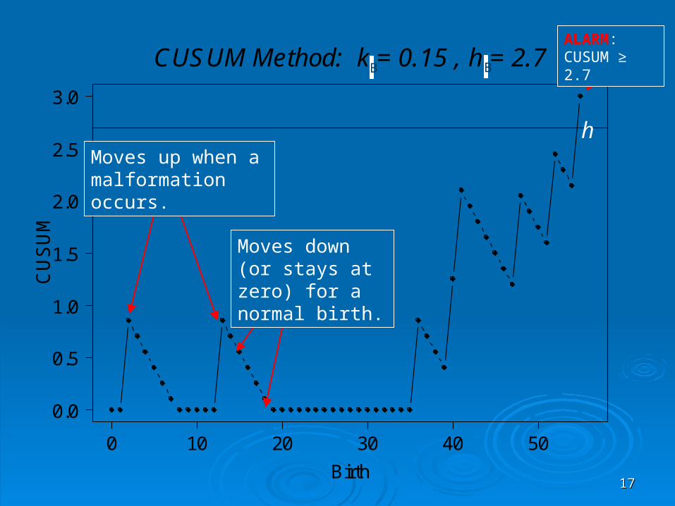
CUSUM Method: k = 0.15 , h = 2.7

Birth

CU

SU

M

h

ALARM: CUSUM ≥ 2.7

Moves up when a malformation occurs.

Moves down (or stays at zero) for a normal birth.

B B

Performance MetricsPerformance Metrics

Charts should be compared based on the average Charts should be compared based on the average number of observations until a signal occurs, the number of observations until a signal occurs, the ANOS.ANOS.

Steady–state random–shift models should be used Steady–state random–shift models should be used when comparing methods. Under this model a shift when comparing methods. Under this model a shift in in pp occurs after the process monitoring has been occurs after the process monitoring has been underway and the shift in underway and the shift in pp may occur at any time. may occur at any time.

1818

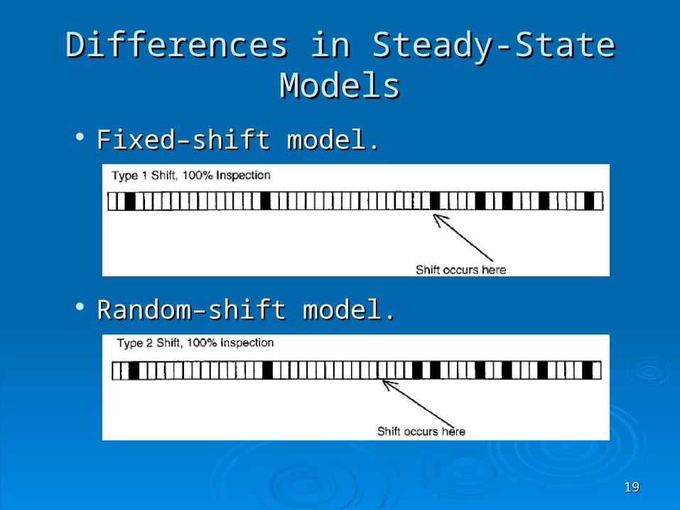
Differences in Steady-State ModelsDifferences in Steady-State Models

Fixed–shift model.Fixed–shift model.

Random–shift model.Random–shift model.

1919

Misconceptions about the Misconceptions about the Geometric CUSUM ChartGeometric CUSUM Chart

For a zero–state analysis, a natural headstart feature For a zero–state analysis, a natural headstart feature is present for the geometric CUSUM chart.is present for the geometric CUSUM chart.

For a steady–state analysis, the geometric CUSUM For a steady–state analysis, the geometric CUSUM chart is considered better than the Bernoulli CUSUM chart is considered better than the Bernoulli CUSUM chart in some cases, but only because the fixed–shift chart in some cases, but only because the fixed–shift model is used.model is used.

2020

Fixed vs. Random–Shift ModelFixed vs. Random–Shift Model

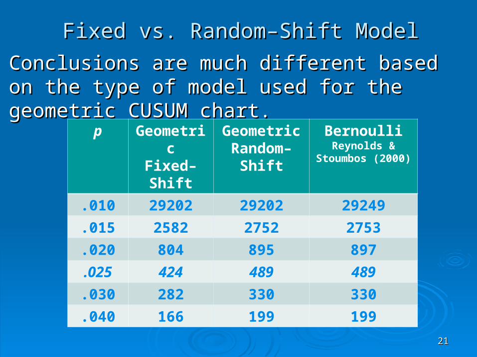
Conclusions are much different based on the type Conclusions are much different based on the type of model used for the geometric CUSUM chart.of model used for the geometric CUSUM chart.

2121

p GeometricFixed–Shift

GeometricRandom–

Shift

BernoulliReynolds &

Stoumbos (2000)

.010 29202 29202 29249

.015 2582 2752 2753

.020 804 895 897

.025 424 489 489

.030 282 330 330

.040 166 199 199

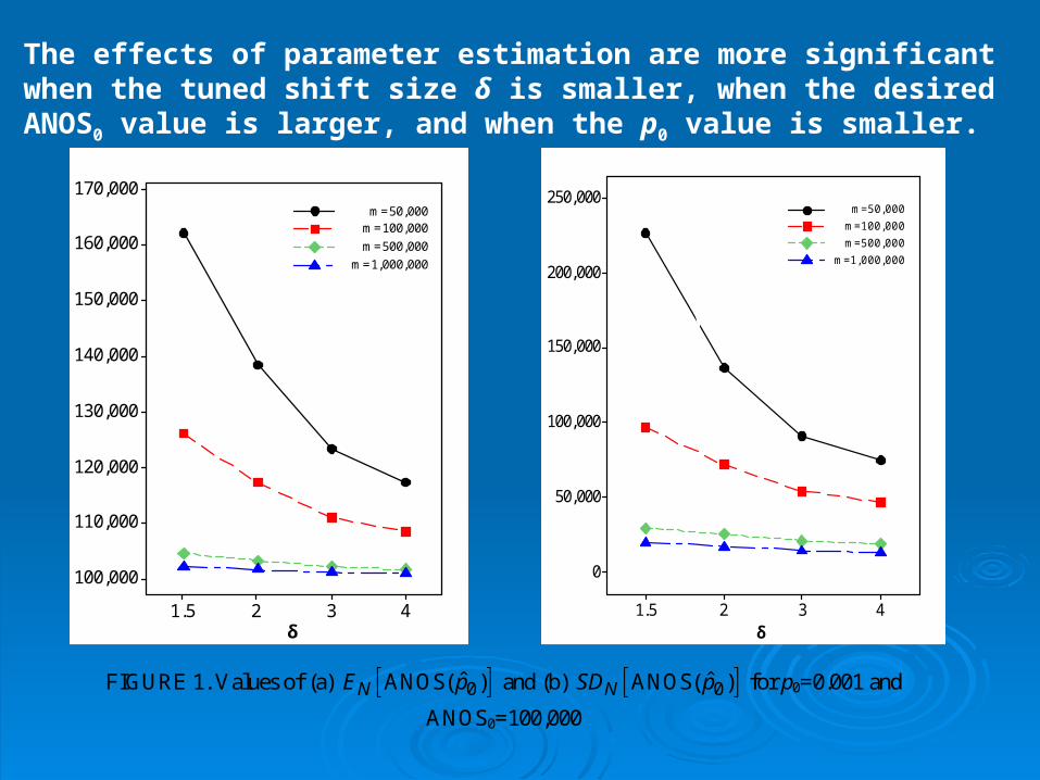
The effects of parameter estimation are more significant when the tuned shift size δ is smaller, when the desired ANOS0 value is larger, and when the p0 value is smaller.

4321.5

170,000

160,000

150,000

140,000

130,000

120,000

110,000

100,000

δ

m=50,000m=100,000m=500,000

m=1,000,000

4321.5

250,000

200,000

150,000

100,000

50,000

0

δ

m=50,000

m=100,000

m=500,000

m=1,000,000

FIGURE 1. Values of (a) 0ˆANOS( )NE p and (b) 0ˆANOS( )NSD p for p0=0.001 and

ANOS0=100,000

(a) (b)

2323

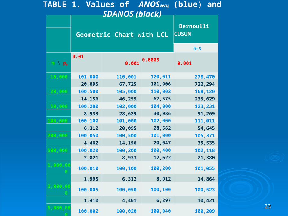
Geometric Chart with LCLBernoulli

CUSUM

δ=3

m \ p0 0.01

0.001 0.0005 0.001

10,000 101,000 110,001 120,011 278,470

20,095 67,725 101,906 722,294

20,000 100,500 105,000 110,002 168,120

14,156 46,259 67,575 235,629

50,000 100,200 102,000 104,000 123,231

8,933 28,629 40,986 91,269

100,000 100,100 101,000 102,000 111,011

6,312 20,095 28,562 54,645

200,000 100,050 100,500 101,000 105,371

4,462 14,156 20,047 35,535

500,000 100,020 100,200 100,400 102,118

2,821 8,933 12,622 21,380

1,000,000 100,010 100,100 100,200 101,055

1,995 6,312 8,912 14,864

2,000,000 100,005 100,050 100,100 100,523

1,410 4,461 6,297 10,421

5,000,000 100,002 100,020 100,040 100,209

892 2,821 3,981 6,561

∞ 100,000 100,000 100,000 100,055

　 0 0 0 0

TABLE 1. Values of ANOSavg (blue) and SDANOS (black)

Two Generalizations of Bernoulli CUSUM ChartTwo Generalizations of Bernoulli CUSUM Chart

Steiner et al. (2000) used a logistic regression model Steiner et al. (2000) used a logistic regression model to let to let pp00 vary from item to item. This is widely used in vary from item to item. This is widely used in the risk-adjusted monitoring of surgical outcomes the risk-adjusted monitoring of surgical outcomes where the health characteristics of patients can vary where the health characteristics of patients can vary widely.widely.

Ryan et al. (2011) extended the approach to the case Ryan et al. (2011) extended the approach to the case where there are more than two outcomes, e.g., where there are more than two outcomes, e.g., manufactured items are classified as good, fair, or manufactured items are classified as good, fair, or bad.bad.

2424

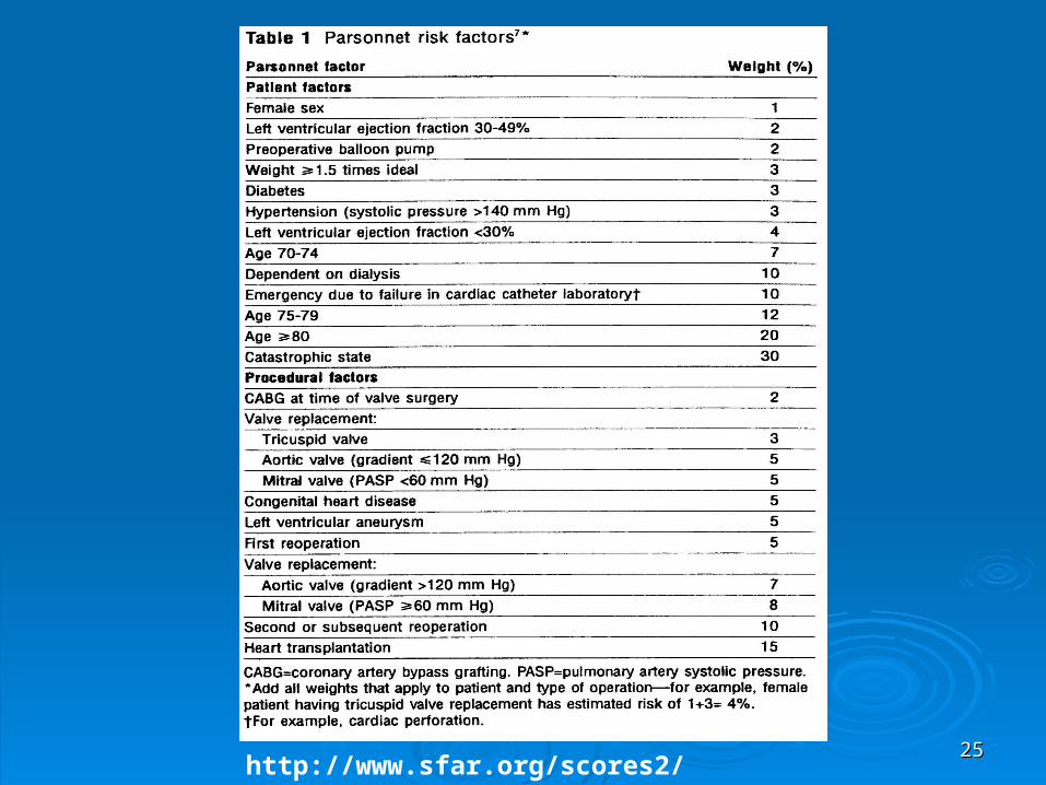
2525http://www.sfar.org/scores2/parsonnet2.html

2626

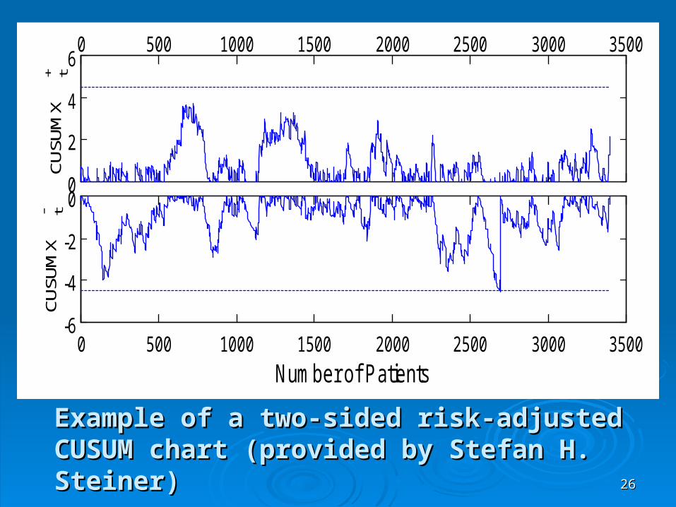
Example of a two-sided risk-adjusted CUSUM Example of a two-sided risk-adjusted CUSUM chart (provided by Stefan H. Steiner)chart (provided by Stefan H. Steiner)

0 500 1000 1500 2000 2500 3000 3500

0

2

4

6CU

SUM

Xt+

0 500 1000 1500 2000 2500 3000 3500-6

-4

-2

0

Number of Patients

CUSU

M X

t-

ConclusionsConclusions It is important to consider the variation in performance It is important to consider the variation in performance

as well as the expected in-control performance of control as well as the expected in-control performance of control charts when parameters are estimated.charts when parameters are estimated.

The Phase I sample sizes required for reliable in-control The Phase I sample sizes required for reliable in-control performance of geometric control charts can be performance of geometric control charts can be impractically large.impractically large.

The steady-state performance of methods for monitoring The steady-state performance of methods for monitoring with Bernoulli data should be evaluated using the with Bernoulli data should be evaluated using the random–shift model.random–shift model.

Using a fixed–shift model has led to conclusions that the Using a fixed–shift model has led to conclusions that the geometric CUSUM chart is better than the Bernoulli geometric CUSUM chart is better than the Bernoulli CUSUM chart for detecting an increase in CUSUM chart for detecting an increase in p p when the when the methods can be designed to be equivalent.methods can be designed to be equivalent.

2727

Conclusions (continued)Conclusions (continued)

The Bernoulli CUSUM chart is much more adversely The Bernoulli CUSUM chart is much more adversely affected by estimation error than the geometric control affected by estimation error than the geometric control chart, requiring much larger Phase I sample sizes.chart, requiring much larger Phase I sample sizes.

Because required sample sizes can be too large to be Because required sample sizes can be too large to be practical, the method of Steiner and MacKay (2004) is practical, the method of Steiner and MacKay (2004) is highly recommended for identifying continuous product highly recommended for identifying continuous product or process variables to monitor in place of the attribute or process variables to monitor in place of the attribute approach. This can lead to more information, much approach. This can lead to more information, much smaller Phase I sample sizes, and greater ability to smaller Phase I sample sizes, and greater ability to detect process changes and to improve the process. detect process changes and to improve the process.

2828

ReferencesReferences Jensen, W. A., Jones-Farmer, L. A., Champ, C. W., and Woodall, W. H. (2006).

“Effect of Parameter Estimation on Control Chart Properties: A Literature Review”. Journal of Quality Technology 38(4), 349-364.

Lee, J., Wang, N., Xu, L., Schuh, A., and Woodall, W. H. (2011), “The Effect of Parameter Estimation on the Upper-Sided Bernoulli CUSUM Charts”, to be submitted to Journal of Quality Technology.

Quesenberry, C. P. (1995). “Geometric Q-chart for High Quality Processes”, Journal of Quality Technology 27, 304-315.

Reynolds, M. R., Jr. and Stoumbos, Z. G. (1999). “A CUSUM Chart for Monitoring a Proportion When Inspecting Continuously". Journal of Quality Technology 31(1), 87-108.

Ryan, A. G., Wells, L.J., and Woodall, W. H. (2011), “Methods for Monitoring Multiple Proportions When Inspecting Continuously”, to appear in the Journal of Quality Technology.

Steiner, S. H., Cook, R. J., Farewell, V. T., and Treasure, T. (2000). “Monitoring Surgical Performance Using Risk-Adjusted Cumulative Sum Charts”. Biostatistics 1, 441-452.

2929

References References (continued) (continued)

Steiner, S. H. and MacKay, R. J. (2004). Effective Monitoring of Processes with Parts Per Million Defective – A Hard Problem! In H. J. Lenz and P.Th. Wilrich (Eds.), Frontiers in Statistical Quality Control 7. Heidelberg, Germany: Springer-Verlag.

Szarka, J. L., III, and Woodall, W. H. (2011), “Performance Evaluations and Comparisons with the Bernoulli CUSUM Chart”, to appear in Journal of Quality Technology.

Szarka, J. L., III, and Woodall, W. H. (2011), “A Review and Perspective on Surveillance of High Quality Bernoulli Processes”, submitted to Technometrics.

Tang, L. C. and Cheong, W. T. (2004). “Cumulative Conformance Count Chart with Sequentially Updated Parameters”. IIE Transactions 36, 841-853.

Yang, Z., Xie, M., Kuralmani, V., and Tsui, K-L. (2002). “On the Performance of Geometric Charts with Estimated Control Limits”. Journal of Quality Technology 34(4), 448-458.

Zhang, M., Peng, Y., Schuh, A., Megahed, F. M., and Woodall, W. H. (2011), “A Reconsideration of Geometric Charts with Estimated Parameters”, submitted to Journal of Quality Technology.

3030