Embed Size (px)
Citation preview
FEDERAL RESERVE BANK OF SAN FRANCISCO
WORKING PAPER SERIES
Monitoring Banking System Connectedness with Big Data
Galina Hale Jose A. Lopez
Federal Reserve Bank of San Francisco
April 2018
Working Paper 2018-01
http://www.frbsf.org/economic-research/publications/working-papers/2018/01/
Suggested citation:
Hale, Galina, Jose A. Lopez. 2018. “Monitoring Banking System Connectedness with Big Data” Federal Reserve Bank of San Francisco Working Paper 2018-01. https://doi.org/10.24148/wp2018-01 The views in this paper are solely the responsibility of the authors and should not be interpreted as reflecting the views of the Federal Reserve Bank of San Francisco or the Board of Governors of the Federal Reserve System.

Monitoring Banking System Connectedness with Big Data
Galina Hale
Jose A. Lopez
Federal Reserve Bank of San Francisco∗
April 23, 2018
ABSTRACT: The need to monitor aggregate financial stability was made clear during the globalfinancial crisis of 2008-2009, and, of course, the need to monitor individual financial firms from amicroprudential standpoint remains. However, linkages between financial firms cannot be observedor measured easily. In this paper, we propose a procedure that generates measures of connectednessbetween individual firms and for the system as a whole based on information observed only at thefirm level; i.e., no explicit linkages are observed. We show how bank outcome variables of interestcan be decomposed, including with mixed-frequency models, for how network analysis to measureconnectedness across firms. We construct two such measures: one based on a decomposition of bankstock returns, the other based on a decomposition of their quarterly return on assets. Networkanalysis of these decompositions produces measures that could be of use in financial stabilitymonitoring as well as the analysis of individual firms’ linkages.
JEL codes: C32, G21, G28
Keywords: financial stability, bank supervision, network centrality, systemic connectedness
∗The views in this paper are solely the responsibility of the authors and should not be interpreted as reflecting theviews of the Federal Reserve Bank of San Francisco or the Board of Governors of the Federal Reserve System. Wethank Tesia Chuderewicz and Shannon Sledz for their excellent research assistance. We benefitted from commentsfrom Fred Furlong, Eric Ghysels, Linda Goldberg, Eric Heitfield, Anna Kovner, James Vickery, two anonymousreferees as well as seminar participants at the Federal Reserve Banks of Dallas and New York and colleagues withinthe Federal Reserve System.
1
1 Introduction
In recent years, the economic literature in several fields has shown increased interest in measuring
and understanding how various economic agents are connected with each other. The literature on
social, trade, industrial, and financial networks has blossomed. Yet, in some fields, and especially
in finance, measuring connectedness between financial firms remains challenging since the data
needed to gauge these linkages are not observed readily or are not available at the appropriate
level of granularity. A key insight into this challenge was provided by Diebold and Yilmaz (2014)
in that they chose to gauge financial firm connectedness using their stock returns as the input
data. They analyze the network implied by their stock return volatility, which neatly avoids data
availability challenges while still capturing the aggregate and idiosyncratic effects of the firms’
interconnectedness.1
The goal of this paper is to develop a procedure that can be used to construct firm-level con-
nectedness measures that rely on as much of the available data for U.S. bank holding companies
(BHCs), have a transparent interpretation, and exhibit desired statistical properties. While we
frame our discussion in terms of measuring the connectedness of these financial firms for various
purposes (with an emphasis on bank supervision and financial stability monitoring), the proposed
approach can be applied readily to other networks of interest, such as industrial sectors. Our proce-
dure generates distinct measures of overall system connectedness and indicators of how individual
entities are both connected to each other and to the system as a whole. The procedure relies on
data that is available at the entity level, and no direct information on actual linkages between
entities is available.
From the perspective of bank supervision, the global financial crisis of 2008-2009 and the subse-
quent regulatory response have brought forth the importance of measuring and monitoring financial
stability and connectedness within (and across) national banking systems.2 A key design element
1The recent network literature has proposed techniques that transform various forms of data into connectednessmeasures. For example, Demirer et al. (2017) also use stock market returns to characterize the high-dimensionalnetwork linking the largest global banks over the period from 2003 to 2014. In contrast, Hale et al. (2016) useinterbank lending exposures to measure the transmission of financial shocks across borders through internationalbank connections.
2Researchers have proposed a wide variety of financial stability measures, such as CoVaR (Adrian and Brunnermeir,2016); see Bisias et al. (2012) for a survey as well as Brave and Lopez (2017) for analysis of specific measures.Connectedness has also been studied via the interbank lending market (Afonso and Lagos, 2015).
2

in such monitoring efforts is in selecting explanatory variables useful for the identification of both
macroprudential (or systemic) and microprudential (or firm-specific) concerns. Theoretically, all
data sources on financial firms are of interest for these activities, but in reality, they all have
particular strengths and weaknesses. For example, focusing on data frequency, we have extensive
quarterly balance sheet data, which provide the most comprehensive and up-to-date summaries of
firm conditions (i.e., asset quality and income). However, these data are available with time lags
and likely too infrequently for use in responding to fast-moving events. At the other extreme, daily
market data is timely and aggregate much current information, but their volatility and tendency
to initially overreact to incoming news limits their usefulness for supervisory monitoring purposes.
Bank supervisors have faced related challenges regarding these data sources for some time; for
example, see the long span of literature from Meyer and Pifer (1970) to Balasubramnian and Palvia
(2018). To date, however, these efforts have been targeted to microprudential supervisory purposes.
Our goal is to develop empirical measures that would be useful for macroprudential monitoring as
well. While many measures of financial stability have been proposed, no one source of banking
data provides a clear measure of interconnectedness for both purposes. In our work, we pay specific
attention to identifying connectedness that arises from common factors affecting all network firms
separately from connectedness that is driven more by the spillover of idiosyncratic shocks.
Our procedure consists of two steps: the decomposition of a BHC outcome variable into com-
ponents of interest, and the network analysis of these components. The decomposition allows us
to extract common factors that affect all firms within the network and, more importantly, identify
idiosyncratic shocks that include any remaining connections between the firms. We propose a num-
ber of approaches on how this decomposition, focusing on dealing with mixed frequency data. The
network analysis can then be applied to any component resulting from the decomposition, with a
particular emphasis on the idiosyncratic terms.
For our proposed measures, we examine bank holding company (BHC) data to study how the
largest U.S. banks were interlinked during the period from 2005 through 2015. The two outcome
measures we analyze are weekly stock returns and quarterly returns on assets (ROA). We decompose
these measures into fitted values and residuals using various regression techniques. We decompose
stock returns using OLS into what we refer to as common and idiosyncratic components using a
3

simple CAPM regression. We decompose ROA into what we refer to as observed and unobserved
components, including both market and firms-specific factors, using a “kitchen-sink” approach with
mixed-frequency data.
We proceed in our network analysis by constructing connectedness measures for idiosyncratic
stock return components using the vector auto-regression (VAR) approach proposed by Diebold
and Yilmaz (2009). However, we use a simple correlation approach to construct connectedness
measures for the observed and unobserved components of ROA since there are insufficient quarterly
observations for VAR estimation. Thus, the measures we construct span quite well the modalities
we describe in our procedure. We provide proof of concept for the resulting measures by comparing
them to other measures of interconnectedness used in the literature, interpreting their dynamics
around crisis times, and comparing them to each other.
To be clear, we are not proposing a new econometric methodology. Our contribution is to
demonstrate how recently developed methodologies can be used to produce useful measures of
connectedness from large amount of available data available at mixed frequencies. For the two steps
of our procedure, we discuss a variety of options available depending on the question of interest,
outcome measures developed, and data constraints. The main innovation of our procedure is that
it allows us to separately analyze connectedness resulting from observable vs. unobservable factors
or from common vs. idiosyncratic components of the outcome variables of interest. As our example
of large banks’ connectedness demonstrate, our procedure produces measures that have intuitive
dynamics and contain additional information relative to other existing measures. Moreover, they
have desired statistical properties of infrequent changes in bank rankings and smooth dynamics.
Interestingly, both stock-market-based and ROA-based measures exhibit substantial growth over
the last two years of our sample, while none of the relevant raw series and other available measures
of banking system risk show such an increase.
We begin by describing our procedure in Part 2. In part 3 we present implementation of
the procedure including data description, as well as construction, description, and analysis of
the measures of systemic connectedness of the U.S. banking system we construct. Summary and
conclusions are in Part 4.
4

2 Methodology for variable decomposition and network analysis
Our implementation procedure consists of two steps. The first step is designed to decompose
the outcome measure into the desired components, and the second step is constructing network
connectedness measures based on these components. In this section, we discuss our procedure in
general terms, and we discuss our specific implementation exercises in Section 3.
2.1 Step 1: Variable Decomposition
Our analysis uses individual firm performance measures - such as weekly BHC stock returns or
quarterly BHC returns on assets - as initial data inputs, as per Diebold and Yilmaz (2009) and
related studies. However, to better examine both the macroprudential and microprudential aspects
of financial system connectedness, we propose standard decompositions that highlight specific ele-
ments of the data.
A common criticism of connectedness measures based on firm stock returns is that they are
dominated by a common component. Within the classic CAPM framework, this caveat is clearly
expressed as
yit = βirmt + εit,
where yit is a firm-specific return and rmt is the return on a market index. This equation can
be applied to each i to obtain firm-specific βi coefficient estimates. The term βirmt represents
the effect of the common market return, and it can be removed to examine the idiosyncratic firm
components (or the εit residuals). Thus, the first type of decomposition we propose is into common
and idiosyncratic components.
The second decomposition we consider is designed to separate out all explainable (or observable)
variation in yit relative to what cannot be explained with available data (i.e., the “unobservable”
component). In notational form, this decomposition is
yit = Z ′tβi +X ′itγi + εit,
where Zt is a set of common variables (such as rmt above) and Xit represents a vector of all
5
explanatory variables available to the researcher. The fitted values, which are a linear combination
of the first two terms, can be labeled as the observable component, and the residual εit term is
the unobservable component. This approach allows us to introduce all available information in a
“kitchen-sink” modeling approach
To conduct these decompositions for our analysis of banking system connectedness, we estimate
individual firm regressions, using OLS techniques if all of the variables are available at the same
frequency.3 This, however, is not commonly the case.
For this reason, Ghysels et al. (2002) propose a mixed-data sampling model based on dis-
tributed lags, commonly known as a MIDAS regression.4 In that framework, higher-frequency
explanatory variables can be included as distributed lags, with a decay parameter estimated either
non-parametrically as an unrestricted MIDAS model (i.e., U-MIDAS) as proposed by Foroni et al.
(2013), or assumed to have a decay of a specific functional form for which parameters are estimated.
For example, if yit is observed quarterly with t indicating a specific calendar date and a subset of
Xit ∈ [Xqit, X
wit ] where the latter is observed weekly, the MIDAS regression can be specified as
yit = Xq′
it βi +
(S∑
s=1
Xw′
i(t−7s)δis
)′γi + εit,
where s is the counter for the weeks in the quarter and S = 13. Again, this equation is intended
to be estimated for each i separately.
An alternative estimation approach is a mixed frequency factor model estimated in state-space
form using the Kalman filter (KF). 5 An advantage of this approach is not requiring any parametric
assumptions; that is, one can simply cast the mixed-frequency data into state-space form and
estimate the model coefficients. Continuing the notation above, suppose the underlying state
process that is driving yit is autoregressive and can be represented with vector αit with transition
equation
αit+1 = Φiαit + Ψiωit,
3Note that we also assume all variables are stationary in our analysis for simplicity.4Asymptotic and other statistical properties of the estimator are reported in Andreou et al. (2010).5See Ghysels et al. (2009) for a comparison and relative merits of the these two estimation methods.
6

where ωit is a transition shock. The measurement equation is then
yit = Aαit +Bxit + εit,
where yit is a vector that includes outcome variable yit as well as any elements of Xit that are
deemed endogenous to the state, while xit is a vector of exogenous variables. εit is a measurement
shock. Aruoba et al. (2009) demonstrate that the estimation process is valid in the cases of missing
data, including data missing due to mixed frequencies. Bai et al. (2013) develop an alternative
approach using a periodic steady-state Kalman filter, as described in Assimakis and Adam (2009).
In this approach, the measurement equation consists of two parts — one at low frequency, and
one at higher frequency that repeats periodically within each low-frequency time period. Bai et al.
(2013) show theoretically and with actual data that this approach produces forecasts similar to
MIDAS, including in small samples.6
The discussion above does not dwell on how the filtering equation for variable decomposition
is selected. The decision might be informed by theory, a specific question that needs to be ad-
dressed, as well as the available data. It is important to emphasize that this decision is key for
the interpretation of the results. For example, it is unlikely that all common components can be
cleanly removed, especially since there are likely to be factors that common to just subsets of the
observations. If desired, principle component analysis or dynamic factor models might be used to
remove common factors that are not directly observed.7 One has to be cautious using such an
approach in the small-scale systems in which idiosyncratic shocks affect system dynamics, because
removing common shocks might remove a portion of idiosyncratic ones. In terms of “kitchen-sink”
approaches, a variety of model-selection methods are available for determining the best fit.
2.2 Step 2: Measuring connectedness
The difficulty in measuring firm connectedness arises from the fact that actual linkages between
firms i and j are not commonly observed. Several approaches have been introduced in the literature
6Real data comparison for macroeconomic variables is conducted by Schorfheide and Song (2009) in the context ofmixed-frequency vector auto-regression. A summary of the variety of approaches to estimate mixed-frequency modelsis also in Foroni and Marcellino (2013).
7These approaches are used in relation to measurement of bank linkages in Kapinos and Mitnik (2016) and Kapinoset al. (2017).
7
using individual firms’ stock returns. The goal is to produce a matrix of linkages with all elements
ij filled, which can then be used as the adjacency matrix in network analysis. For example, the
simplest and most straightforward approach is to compute pairwise correlations for each pair of
firms. Another approach is to use a vector autoregression (VAR) model to estimate the effects of
firm i on firm j and define connectedness via forecast error variance decomposition or through a
generalized impulse response function. VAR, of course, needs to be identified, and Diebold and
Yilmaz (2009) propose to identify it with a shrinkage estimator using the elastic net.8
Other approaches to measure the systemic risks of financial firms include conditional value-
at-risk (or CoVaR) by (Adrian and Brunnermeir, 2016), Marginal Expected Shortfall (or MES)
by (Acharya et al., 2012) and the closely related Systemic Risk (or SRISK) by (Acharya et al.,
2010; Brownlees and Engle, 2017), and the Distressed Insurance Premium (or DIP) by (Huang
et al., 2009, 2012). Since none of these approaches are able to produce explicit measures of linkages
between firms i and j, we describe the correlation and the VAR approaches.
Correlation We can construct a matrix of pairwise correlations for the series of interest between
firms i and j at a point in time, and we can use rolling windows over the full data sample to
create a dynamic network. These correlations can be collected into a correlation matrix, which
can be interpreted as adjacency matrix for the network, with two modifications. First, diagonal
elements need to be replaced with zeros. Second, negative elements are not meaningful in the
adjacency matrix. Thus, depending on the application, they can be replaced either with their
absolute values if negative linkages are viewed as important as positive ones (such as, for example,
in social networks), or zeros if negative linkages are not as important. If the goal is to measure
contagion, one may argue that negative linkages actually provide insurance and reduce contagion,
and definitely do not contribute to contagion spread. Thus, for our analysis, it might make sense
in systemic risk analysis to replace negative linkages with zeros, which would amount to ignoring
any effects of insurance or diversification and thus treating it as a conservative adjustment.
There are two main drawbacks of the correlation approach. First, it is entirely backwards-
looking in that observed correlations between past values may not be informative of how correlated
they might be going forward. Second, the correlation matrix is symmetric, which means the network
8This approach is also implemented in Diebold and Yilmaz (2012); Demirer et al. (2017).
8

described by the resulting adjacency matrix is not directional. Accordingly, we cannot distinguish
between a firm’s impact on the system and its vulnerability to the system.
VAR The VAR approach addresses both main drawbacks of the correlation approach. First,
by estimating a VAR, we can forecast future values of the outcome measure, compute forecast
errors, and decompose the error variance as a measure of linkages. While the estimation still
relies on past data, at least this approach has a forecast component that makes it predictive and
not strictly backward-looking. Second, variance decomposition matrix is not symmetric, allowing
us to construct a directional network of linkages and thus measure firm impact and vulnerability
separately. Given that components of the variance decomposition matrix are by definition between
zero and one, the matrix of the variance decomposition can be used directly as adjacency matrix
upon removal of the diagonal.
Upon constructing the adjacency matrix A using one of the methods described above, we con-
struct measures of system connectedness, such as the network density (D) measure, and “systemic
importance” measures for each institution, such as the degree centrality (dc) for directed and undi-
rected networks. Formally, these measures are defined as follows:
D =2∑
i
∑j 6=i aij
N(N − 1), (1)
dci =∑j 6=i
aij , (2)
where aij is an element of A, and N is the number of firms. The network density measure is
intuitively the average value of the off-diagonal cells of the matrix, such that a sparse matrix has
a low D value and a highly-populated matrix has a high D value. The degree centrality measure
similarly adds the values across the row for firm i, measuring the size of the firm’s connectedness
within the system. For interpretation, in case of correlation approach, it might be useful to divide
the dci measure by N − 1 to obtain average systemic importance of a given firm that is between 0
and 1 by construction.
A directed (or asymmetric) network allows us to distinguish directional degree centrality: out-
degree (odci) and in-degree (idci), which can be interpreted, respectively, as the impact of firm i on
9

the rest of the system and the vulnerability of firm i to shocks coming from the rest of the system.
In notation,
odci =∑j 6=i
aij , (3)
idci =∑j 6=i
aji, (4)
As before, odci is a row sum measure, but idci is a column sun measure. Note that the odci impact
measure need not equal the idci vulnerability measure, because the contribution of i to j’s forecast
error variance need not be the same as the contribution of j to i’s forecast error variance.
If the dynamics of a network measure is of interest, these calculations can be repeated for rolling
windows of the outcome measure decomposition. Note that by construction, the D network density
measure is bounded to the unit interval, regardless of how the linkages are computed. Similarly,
the idci measure remains within the unit interval since it measures the total share of forecast error
variance for firm i that is explained by all other firms. In contrast, the dci and odci measures can
sum to more than one.
3 Implementation
Having described our procedure, we now turn to the concrete example of its implementation. Our
example is measuring connectedness and systemic importance in the network of large banks. We
first describe our data, then demonstrate an application with two different outcome measures: stock
returns, which we measure weekly, and returns on assets (ROA), which are available quarterly.
With stock returns which can be measured at any frequency, we don’t have a mixed frequency
problem, and therefore employ simple linear regression to obtain our decomposition. Here we
focus on common and idiosyncratic components interpretation of decomposition and estimate an
augmented CAPM regression with five Fama-French factors (French and Fama, 1992) to separate
market factors from idiosyncratic ones. With the strong common component, we proceed with the
network analysis of the residual from this decomposition, the idiosyncratic component.
With ROA, which is available quarterly, we have explanatory variables that we would like to
include in the decomposition that can be measured at higher frequency. Thus, we employ MIDAS
10

approach to decompose ROA.9 Here we employ a kitchen-sink approach, interpreting decomposition
as resulting in observed and unobserved components of the ROA. We proceed to analyze both the
observed and the unobserved components.
3.1 Data
Bank supervision is a critical component of monitoring and maintaining the safety and soundness of
the U.S. banking and financial system. Dating back to the creation of the Office of the Comptroller
of the Currency (OCC) in 1864, bank examiners have collected data on-site and through reporting
forms to assess compliance with federal banking regulations (White, 2011). Starting in 1869,
balance sheet data collection became more standardized with the development of the “call” report
of condition, which are now more commonly known as the Call Reports. After the Bank Holding
Company Act of 1956, the Federal Reserve began collecting consolidated BHC data, with the
Y9 consolidated reporting forms starting in 1978. All of this data, in conjunction with on-site
examinations and other supervisory work, assists in the creation of supervisory bank ratings, which
are known as CAMELS for commercial banks and RFI/C(D) ratings for BHCs. Statistical models
that summarize supervisory information and correlate it with supervisory outcomes, such as rating
changes and bank failures, date back to the mid-1970s and are in wide use currently (King et al.,
2006).
In addition to supervisory data, market-based data is available for analysis on the largest BHCs.
Pettway and Sinkey (1980) proposed using BHC stock returns for monitoring their financial con-
ditions. Krainer and Lopez (2004, 2008) provide evidence using ordered logit models that both
supervisory and market-based data provide leading indicators of changes in BHC supervisory rat-
ings. Berger et al. (2000) report similar findings, but highlight that supervisory ratings are generally
less accurate than market-based indicators in predicting future changes in bank performance, ex-
cept when these assessments occurred just after a recent on-site bank examination. All of these
efforts have focused on the microprudential goals of monitoring bank-level safety and soundness as
well as allocating resource to do so. Since the financial crisis, macroprudential concerns have arisen
and been partly addresses with stress-testing of the largest BHCs (Hirtle and Lehneart, 2015). Our
9We decided in favor of MIDAS over state-space approach because of the short time span for our data analysis.
11
efforts here work with roughly the same set of firms to derive macroprudential summary measures
of banking system vulnerability and microprudential measures of firms’ systemic importance.
We focus on the 27 large U.S. BHCs that have been subject to the Federal Reserve’s stress-
testing and have data available from 2002 to 2017, listed in Table 1. This choice of a balanced
panel is intentional to allow for the network modeling. This sample includes largest, systemically
important firms that jointly account for over 75% of U.S. banking assets. We use various data
sources in our analysis, which are divided into balance sheet variables and market-based variables.
Our main market-based data is the daily stock returns of the sample, BHCs, which we aggregate to
the quarterly frequency. Note that we do not merger-adjust these returns, even in light of the large
and significant BHC mergers that occurred during 2008 and 2009. Our rationale here is to focus
on the specific firms involved in the Federal Reserve’s stress-testing program and their network
connectedness. Finally, we use S&P 500 stock market returns at the weekly frequency, effective
federal funds rate as reported by the Federal Reserve, as well as five market-wide Fama-French
factors from Kenneth French.
We collect consolidated balance sheet data for the sample BHCs from the Y9-C reporting form,
which is made publicly available on a quarterly basis.10. From this source, we use firm’s total assets,
income, as well as non-performing loans (NPLs).
3.2 Measure 1: Connectedness based on stock returns
Our first example is interconnectedness of BHC’s stock returns. These are available at any fre-
quency, but we are not necessarily interested in intraday and day-to-day fluctuations, for this
reason we choose weekly returns, but computing log change in stock prices from Friday close to
Friday close. Existing measures of stock-return-based interconnectedness are frequency criticized
for having a larger common component. We can address this criticism using our decomposition into
common and idiosyncratic components. For each bank i, we will estimate an augmented CAPM
regression as follows
rit = αi + β1irSPt + β2ir
FFt + β3iSMBt + β4iHMLt + β5iRMWt + β6iCMAt + εit,
10https://www.federalreserve.gov/apps/reportforms/reportdetail.aspx?sOoYJ+5BzDal8cbqnRxZRg==
12

where rit is the weekly stock return for firm i; rSP is a weekly return on S&P 500, rFF is federal
funds rate, while the rest of the controls are market-wide Fama French factors. To allow for βs to
vary over time, we estimate this regression for a 3-year windows from 2002 through 2017, which we
roll forward quarterly.
For almost all banks all of the coefficients estimated are of expected sign and statistically
significant. Figure 1 shows raw returns, fitted, and residual values for Wells Fargo, as an example,
since April 2016. We can see that both common and idiosyncratic factors play an important role in
the dynamics of this bank’s stock returns. The share of variance explained by the market factors
(regression R2) for the last rolling window is reported for all banks in Figure 2. We can see that it
varies from 30-50% for foreign and processing banks to as high as 80% for large and regional banks.
Coefficients for each rolling window and each bank on all the variables included in the regression
are reported as time series in Appendix figure A1.
Given that the fitted values only vary across banks because of differences in βs, we focus on
the residuals for the analysis of connectedness. That is, the idiosyncratic component. It should
be made clear here, that the term “idiosyncratic” is used vaguely in this case, given that there
might be banking-sector-specific common factors that will be manifested as connectedness of the
residuals. There are two reasons we choose not to remove such factors in this specific example. First
is technical — given that we are dealing with a network of only 27 institutions, removing common
factors by extracting principle components or including sector stock index in the regression has a risk
of removing truly idiosyncratic component. Second, from the regulatory point of view, correlated
response of all institutions to the same shock is as relevant as a truly idiosyncratic contagion from
one institution to another.
To construct connectedness of the idiosyncratic component of stock returns at weekly frequency,
we estimate a VAR using elastic net shrinkage estimator. A similar implementation is conducted
by Demirer et al. (2017) for 100 largest global banks. Following similar methodology, we measure
connectedness as variance decomposition of forecast one-quarter-ahead error.11 To construct dy-
namic networks, we estimate the VAR for the same 3-year windows rolling quarterly, as we used
for the regression decomposition.
11One alternative is to use impulse response functions, as in Grant and Yung (2017).
13

The results for the last rolling window ending in December 2017 are reported as an adjacency
matrix in Figure 3. We can observe that the most connected pair are Credit Suisse and Deutsche
Bank, while the most connected cluster is Credit Suisse, Deutsche Bank, BBVA, and Barclays.
This makes sense, because all these are foreign banks and have the largest idiosyncratic component
that likely loads on a common European factor. Toronto-Dominion bank, on the other hand, is the
least connected to the rest of the system. Time series of individual bank impact and vulnerability
measures for the four largest banks are shown in Appendix Figure A2.
The dynamics of the network are quarterly, because we roll the estimation window quarterly.
Overall density is presented in Figure 4, where we compare density of the network of the idiosyn-
cratic component with that of the raw stock market returns (constructed using the same VAR
approach). We can see that the contribution of the common component makes density of raw
returns networks very hight throughout the sample. For the idiosyncratic returns we can see much
more pronounced dynamics — an increase in network connectedness during the Global Financial
crisis that started in the second half of 2007 as well as a pronounced increase in the last two years.
This recent increase is most likely reflecting common response of the banking system to actual and
expected regulatory changes in the last couple of years.
This connectedness is not the same for all banks — Figures 5 and 6 shows measures of impact and
vulnerability, respectively, by bank business group.12 We find that during the global financial crisis
the increased connectedness was limited to the largest four banks (Bank of America, Wells Fargo,
Citigroup, and JP Morgan), and regional banks. Connectedness of other banking groups reached
the level similar to that of four largest banks in 2009. This makes sense, because this is exactly
when regulatory treatment of investment banks, processing banks, and foreign banks’ affiliates was
made similar to that of the largest four banks. In recent years, the impact of investment banks
seems smaller than that of other groups, while vulnerability is lowest for foreign banks.
12Remember that impact and vulnerability here are defined narrowly as outdegree and indegree, respectively. Big4banks are BAC, C, JPM, WFC. Processing banks are BK, NTRS, STT. Foreign banks are BBVA, BCS, CS, DB,TD. Regional banks are BBT, CMA, FITB, HBAN, KEY, MTB, PNC, RF, STI, USB, ZION.
14

3.3 Comparing to other market-based measures
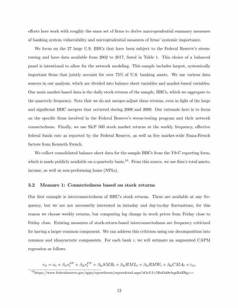
To see whether our approach yields estimates that are both reasonable and not spanned by existing
measures, we compare our measure to other stock-return-based measures commonly used in the
literature. Figure 7 plots standardized and normalized versions of our measure as well as averages
across banks of the three measures: conditional value-at-risk or CoVaR (Adrian and Brunnermeir,
2016) for each firm i, Systemic Risk or SRISK (Acharya et al., 2010; Brownlees and Engle, 2017), and
Distressed Insurance Premium or DIP (Huang et al., 2009, 2012). These measures are commonly
available for only 11 out of our 27 banks. Thus, we repeat our entire procedure for the same 11
banks so that we have a consistent comparison. We can see that our measure is a bit less volatile
but generally has similar dynamics to other measures until end of 2015, when our measure started
to diverge from other market-based measures. Thus, we find that our measure is consistent with
others but also provides additional information.
3.4 Learning from crisis times
Lehman crisis presents an interesting case study. While all banks performed poorly, and some
failed, most of the dynamics of their stock returns are captured by market measures. Some of the
developments, however, has been idiosyncratic. For example, only Citigroup and Bank of America
received bail-out funds from the Targeted Investment Program at the end of 2008 and early in
2009. At the same time, investment banks Goldman Sachs and Morgan Stanley were converted to
Bank Holding Companies which gave them access to the same bailout funds, but with the same
regulatory strings attached, as commercial banks.
These development are reflected in our connectedness measure, as shown in Figure 8. We can
see that Bank of America and Citigroup had a high impact measure on the rest of the system
starting the beginning of the crisis in 2007Q3 and before Lehman collapse in 2008Q3. Thus, one
may argue, these were the right banks to be subject to bailout. We can see that following the
bailout the banks became less connected, especially by 2009Q3, when they were less connected
than other banks. In fact, while connectedness of other banks increased slightly through the crisis
period, following the bailout, impact of Bank of America and Citigroup declined, indicating that
markets started to view them as being apart from the rest of network.
15

Investment banks were designated as BHCs in the second half of 2008. We can see that his lead
to substantial increase in their impact relative to the previous period. As we have seen in previous
discussion, by 2011 these two banks’ connectedness measures were not substantially different than
those of the other large banks. In Figure 8 we can see clearly, however, that this convergence
started in mid-2009.
3.5 Measure 2: Connectedness based on ROA
Our second example is interconnectedness of observed and unobserved components of banks’ return
on assets (ROA), Rit. ROA is measured as a ratio of a bank’s quarterly income to the average of
bank’s assets over last three preceding quarters. As such, Rit is measured at quarterly frequency.
We use the kitchen-sink approach to separate observed portio of the ROA for each bank from
unobserved, acknowledging that market movements might affect book income. To be clear, the
kitchen-sink approach does not imply causal effect of explanatory variables on the outcome variable,
we simply are trying to get the best fit regression given the data available. In addition to the same
set of market factors we used in the first example, which we continue to measure at weekly frequency,
we add a measure of non-performing loans (as a share of assets), Nij , which is available quarterly.
Because of this data structure, we have to use mixed-frequency approach, which we implement
with U-MIDAS, an unrestricted form of MIDAS regression which does not require parametric
assumptions.13
After extensive pretesting and observing constraints on data availability, we settled on the
following regression equation, for 16 banks, starting 2002, estimated individually for each firm i:
Rit = αi + βiNit + γi
S∑s=1
(δ1sirKBWt + δ2sir
FFt ) + εit, (5)
where ROAit is the quarterly return on assets for firm i; Nit is a quarterly ratio of non-performing
loans to total assets; rKBWt is the weekly return on a large banks index KBW; rFF
t is weekly
effective federal funds rate as defined above. We estimate this equation via U-MIDAS for the 16
banks for which we have sufficient balance-sheet data going back to 2012. Due to lower frequency
of the dependent variable, we estimate one equation for each bank for the entire time period and
13We make use of R code produced by Ghysels et al. (2016) to estimate U-MIDAS.
16

construct fitted and residual values. Even though this specification is parsimonious, it includes
bank-specific, sector-specific, and macroeconomic factors that fit the ROA quite well as shown by
R2 in Figure 10. Using the example of Wells Fargo, Figure 9 shows the decomposition of the ROA
into observed and unobserved components. We can see that the model captures quite well negative
returns at the peak of the crisis in 2008Q4, leaving very little to the residual. Most likely, this is
due to a combination of market impact via KBW index and bank-specific NPLs. Overall we can see
that the volatility of observed and unobserved components of ROA are quite similar. Coefficients
on all variables in the regression for all banks are reported in Appendix Figure A3.
Given that regressions include bank-specific factors, we are interested in connectedness of both,
fitted values (observed component) and residuals (unobserved component). For this case, given
quarterly data and short time frame, we resort to simple correlations as measures of connectedness.
To obtain dynamic networks, we construct correlations over 16-quarter rolling windows.
Remember that correlation methods produces a non-directional network, which is why adjacency
matrices from the last rolling window reported in Figures 9 and 10 for observed and unobserved
components, respectively, are symmetric. Because we are interested in the measure of banking
system fragility, only positive correlations are threatening to the system, either as response to
common shocks or as contagion arising from idiosyncratic shocks. Negative correlations, instead,
would serve as mitigating factors that one can think of diversification or insurance. For this reason,
we replace negative correlations with zeros instead of replacing them with absolute values.
We find that observed components are quite highly connected for a number of banks and a
negative correlation arises very infrequently. As an example, Figure 11 shows the adjacency matrix
for the last rolling window ending 2017Q4. The least connected banks in terms of the observed
component are JP Morgan, NTRS, and BBVA. Given that they all face the same sectoral and
macroeconomic conditions, this indicates that either the dynamics of their NPLs is quite different
of that of other banks, or the response of their returns to sectoral and macroeconomic factors is
different from the rest of banks in the network. BBT, Bank of America, and Citibank are, on the
other hand, quite highy conected with the rest of the network.
The unobserved components have a number of negative correlations and are generally less
connected than observed components. Figure 12 shows the adjacency matrix for the last rolling
17

window. Again, JP Morgan, NTRS, and BBVA are the least connected (although unobserved
component of BBVA is highly connected with that of Citigroup). Combined with previous finding,
this shows that these banks’ ROAs have moved differently in the last four years of our data from
the rest of the banks in the network. Highly connected unobserved components are apparent for
Key Bank and MTB. One can only see a highly-connected cluster in the network: Wells Fargo,
PNC, US Bank, and Key Bank. Another cluster consists of CMA, HSBC, and MTB.
Looking at the dynamics of connectedness for the four large banks, as shown in Figures 13
and 14, for observed and unobserved connectedness, respectively. We can see that JP Morgan
stands out, with dynamics completely different from three other large banks, for which the dynamics
are more or less the same. Interestingly, for the other three large banks we observe an increase in
unobserved connectedness in recent year similar to what we observed for the market return-based
connectedness, our first measure. This is reassuring, because we applied different methodologies to
different variables in every step of our procedure.
This increase in connectedness in the last two years is also visible in the overall density, as shown
in Figure 15. We can see that, despite declining or steady connectedness of raw ROAs in recent
years, both observed and unobserved components’ connectedness is on the rise. While for observed
connectedness the level is still about half of what we observed during the crisis, for unobserved
connectedness current level is nearly as high as the peak in early 2010. Again, this is a similar
pattern to the one resulting from Measure 1, suggesting that some underlying connectedness in
bank performance that is not easily measured otherwise, is on the rise.
3.6 Connectedness between observed and unobserved components
We would like to discuss one extension to our analysis. So far, we considered each component result-
ing from our decomposition as completely independent. While it is true that by construction our
decomposition yields components that are orthogonal to each other for each individual institution,
observed and unobserved components, for example, may be connected across institutions. That
is, if we create a 2N ∗ 2N adjacency matrix of both observed and unobserved components, there
might be interesting linkages in the off-diagonal N ∗N submatrices. These elements are important
to measure to assess overall systemic importance of an institution.
18

We conduct this exercise for observed and unobserved components of ROA that we computed for
our second measure. For these, we compute 32*32 correlation matrix for observed and unobserved
components for our 16 banks, using the same 16-quarter rolling window. Because the matrix is
symmetric, we only need to analyze one off-diagonal submatrix which we can view as a cluster in
the network. Figure 16 shows this submatrix for the last rolling window in our sample. We can
see that most correlations are either negative, zero, or very small. Only a handful of correlations
stand out — it appears that unobserved component (residuals) for JP Morgan is correlated with
the observed component (fitted) for a number of banks and observed component for JP Morgan
is correlated with unobserved component for the same set of banks. This tells us that systemic
importance of JP Morgan is, in fact, larger than measured by its connectedness in observed and
unobserved component networks when viewed separately. We can also note that observed and
unobserved components of BBT and NTRS ROAs are highly correlated with each other. Finally,
unobserved component with NTRS is correlated with observed components of most other banks in
the network.
Figure 17 shows the dynamics of this cluster density (that is, average correlation across all
elements of the off-diagonal submatrix, for which we replaced negative numbers with zeros) and
compares it with the density of observed and unobserved clusters that we described before. We
find, as we expected, that correlations between observe and unobserved components tend to be
substantially lower than within observed and across unobserved components across banks. Thus,
in our case, analyzing connectedness of observed and unobserved components separately is not a
bad approximation.
4 Summary and conclusions
In this paper we propose a procedure that allows us to construct systemic connectedness measures
on the basis of the data that are only available at individual level, not individual-pair level. We
pay particular attention to methods available to extract a common component, including recently
developed techniques for the analysis of mixed frequency data. We implement our procedure to
construct two measures of U.S. banking system connectedness.
19

Bank supervision is an important public policy concern that dates back to at least the 1860s in
the United States. While the firm-specific (or microprudential) issues remain as relevant as ever,
policymakers have added macroprudential (or systemic) concerns to their supervisory responsibili-
ties since the global financial crisis. Our measures of network density and of firm-specific systemic
impact and vulnerability should be of broad usefulness to bank supervisors.
Our methodological proposal consists of two steps that combine several recent developments in
network analysis for supervisory use. The first step based on mixed-frequency regression techniques
allow us to decompose firm performance measures into a fitted (common or observed) component
and a residual (idiosyncratic or unobserved) component. While we use a particular regression
specification, other users might choose to select other variables or other specification to achieve a
decomposition that suits their purpose and data structure. For bank supervisors, such decompo-
sition provides information when new developments outside of their standard scope of monitoring
may be arising and may require additional resources. For this study, we examine weekly BHC stock
returns and quarterly ROAs, but other measures — such as credit risk or loan losses — could be
similarly analyzed. The isolation of the unobserved component is of particular interest as it reflects
factors that are not measured otherwise.
The second step of our procedure is based on network analysis, mainly of the type proposed
by Diebold and Yilmaz (2009, 2012, 2014), as well as simple correlations. We examine several
measures of aggregate and firm-specific network connectedness to provide supervisory insights on
the current state of banking system stability. There are various measures and analytics available,
and we propose the use of a representative set of them; however, we acknowledge that other users or
other policy questions might require the use of other measures. We see this flexibility as a strength
of our proposed framework.
Finally, we show that measures we construct are meaningful — in terms of comparison with other
existing measures and their dynamics around crisis times — and contain additional information
relative to other measures. Specifically, both measure we construct, using different variables and
approaches at every step of the procedure, show a substantial increase in the last two years of our
sample. This increase is absent from any raw data series or other systemic risk measures available
for the banking system.
20

References
Acharya, V. V., Engle, R. F., and Rchardson, M. P. (2010). Capital shortfall: A new approach
to ranking and regulating systemic risk. American Economic Review: Papers and Proceedings,
102:59–64.
Acharya, V. V., Pedersen, L. H., Philippon, T., and Rchardson, M. P. (2012). Measuring systemic
risk. CEPR Working Paper.
Adrian, T. and Brunnermeir, M. K. (2016). CoVaR. American Economic Review, 106(7):1704–41.
Afonso, G. and Lagos, R. (2015). Trade dynamics in the market for federal funds. Econometrica,
83:263–313.
Andreou, E., Ghysels, E., and Kourtellos, A. (2010). Regression models with mixed sampling
frequencies. Journal of Econometrics, 158(2):246–61.
Aruoba, S., Diebold, F., and Scotti, C. (2009). Real-time measurement of business conditions.
Journal of Business and Economic Statistics, 27(4):417–27.
Assimakis, N. and Adam, M. (2009). Steady state kalman filter for periodic models: A new
approach. International Journal of Contemporary Mathematical Sciences, 4:201–18.
Bai, J., Ghysels, E., and Wright, J. H. (2013). State Space Models and MIDAS Regressions.
Econometric Reviews, 32(7):779–813.
Balasubramnian, B. and Palvia, A. (2018). Can short sellers inform bank supervision? Journal of
Financial Services Research, 53(1):69–98.
Berger, A., Davies, S., and Flannery, M. (2000). Comparing market and supervisory assessments of
bank performance: Who knows what when? Journal of Money, Credit, and Banking, 32(3):641–
667.
Bisias, D., Flood, M., Lo, A., and Val, S. (2012). A survey of systemic risk analytics. Annual
Review of Financial Economics, 4:255–296.
21

Brave, S. and Lopez, J. (2017). Calibrating macroprudential policy to forecasts of financial stability.
Federal Reserve Bank of San Francisco WP 2017-17.
Brownlees, C. and Engle, R. (2017). SRISK: A conditional capital shortfall measure of systemic
risk. Review of Financial Studies, 30(1):48–79.
Demirer, M., Diebold, F., Liu, L., and Yilmaz, K. (2017). Estimating global bank network con-
nectedness. National Bureau of Economic Research WP 23140.
Diebold, F. and Yilmaz, K. (2009). Measuring financial asset return and volatility spillovers with
application to global equity markets. Economic Journal, 119(534):158–171.
Diebold, F. and Yilmaz, K. (2012). Better to give than to receive: Predictive measurement of
volatility spillovers. International Journal of Forecasting, 28(1):57–66.
Foroni, C., Macellion, M., and Schumacher, C. (2013). Unrestriced mixed data sampling (MIDAS):
MIDAS regressions with unresticted lag polynomials. Journal of the Royal Statistical Society:
Series A (Statistics in Society), 178(1):57–82.
Foroni, C. and Marcellino, M. (2013). A survey of econometric methods for mixed-frequency data.
Norges Bank WP 2013/06.
French, K. R. and Fama, E. (1992). The cross-section of expected stock returns. Journal of Finance,
47(2):427–465.
Ghysels, E., Kvedaras, V., and Zemlys, V. (2016). Mixed Freqency Data Sampling Regression
Models: the R Package midasr. Journal of Statistical Software, 72(4).
Ghysels, E., Santa-Clara, P., and Valkanov, R. (2002). The MIDAS Touch: Mixed Data Sampling
Regression Models. Mimeo.
Grant, E. and Yung, J. (2017). The double-edged sword of global integration: Robustness, fragility
& contagion in the international firm network. FRB Dallas Globalization and Monetary Policy
Institute Working Paper 313.
22

Hale, G., Kapan, T., and Minoiu, C. (2016). Crisis transmission through the global banking
network. IMF Working Paper 16/91.
Hirtle, B. and Lehneart, A. (2015). Supervisory stress tests. Annual Review of Financial Economics,
7(1):339–355.
Huang, X., Zhou, H., and Zhu, H. (2009). A framework for assessing the systemic risk of major
financial institutions. Journal of Banking and Finance, 33:2036–49.
Huang, X., Zhou, H., and Zhu, H. (2012). Assessing the systemic risk of a heterogeneous portfolio
of bbanks during the recent financial crisis. Journal of Financial Stability, 8(3):193–205.
Kapinos, P., Kishor, K. A., and Ma, J. (2017). Dynamic comovements among banks, systemic risk,
and the macroeconomy. mimeo.
Kapinos, P. and Mitnik, O. A. (2016). A top-down approach to stress-testing banks. Journal of
Financial Services Research, 49:229–264.
King, T., Nuxoll, D., and Yeager, T. (2006). Are the causes of bank distress changing? can
researchers keep up? Federal Reserve Bank of St. Louis Review, 88:57–80.
Krainer, J. and Lopez, J. (2004). Incorporating equity market information into supervisory moni-
toring models. Journal of Money, Credit, and Banking, 36:1043–1067.
Krainer, J. and Lopez, J. (2008). Using securities market information for bank supervisory moni-
toring. International Journal of Central Banking, 4:125–164.
Meyer, P. and Pifer, H. (1970). Prediction of bank failures. Journal of Finance, 25(4):853–868.
Pettway, R. H. and Sinkey, J. (1980). Establishing on-site bank examination priorities: An early-
warning system using accounting and market information. Journal of Finance, 35(1):137–150.
Schorfheide, F. and Song, D. (2009). Real-Time Forecasting with a Mixed-Frequency VAR. Journal
of Business and Economic Statistics, 33(3):366–80.
White, E. (2011). ”to establish a more effective supervision of banking”: How the birth of the fed
altered bank supervision. National Bureau of Economic Research WP 16825.
23

Table 1: Banks included in the sample
Ticker Bank Name Total Assets in MIDAS?
AXP American Express Company 181 N
BAC Bank of America 2,281 Y
BK Bank of New York Mellon 372 N
BCS* Barclays 158 N
BBT BB&T Corporation 2212 Y
BBVA* BBVA Compass Bancshares 87 Y
COF Capital One Financial 366 N
C Citigroup 1,842 Y
CMA Comerica Incorporated 7 2 Y
CS* Creidt Suisse Group AG 141 N
DB* Deutsche Bank US 148 N
FITB Fifth Third Bancorp 142 N
GS Goldman Sachs Group 917 N
HBAN Huntington Bancshares Incorporated 104 Y
JPM JPMorgan Chase & Co. 2,534 Y
KEY KeyCorp 138 Y
MTB M&T Bank Corporation 119 Y
MS Morgan Stanley 852 N
NTRS Northern Trust Corporation 139 Y
PNC PNC Financial Services Group 381 Y
RF Regions Financial 125 N
STT State Street Corporation 238 Y
STI Suntrust Banks 207 Y
TD* TD Group US Holdings 381 N
USB U.S. Bancorp 462 Y
WFC Wells Fargo & Company 1,952 Y
ZION Zion Bancorporation 66 Y
Note: Total assets are in billion USD as of 2017Q4. * Indicates only U.S. assets of foreign-owned
companies are reported. “In MIDAS?” indicates whether or not the bank is included in the MIDAS
measure sample.
24

Figure 1: Stock returns decomposition for Wells Fargo
‐0.075
‐0.025
0.025
0.075
0.125
Raw returns Fitted Values Residuals
Note: Reported are weekly stock returns as well as fitted values and residuals from the CAPMregression estimated for the last 3-year rolling window. Only last 6 quarters are shown for
exposition purposes.Source: Bloomberg and authors’ calculations.
25

Figure 2: R2 from rolling CAPM regression (last rolling window)
AX
P
BA
C
BB
T
BB
VA
BC
S
BK C
CM
A
CO
F
CS
DB
FIT
B
GS
HB
AN
JPM
KE
Y
MS
MT
B
NT
RS
PN
C
RF
ST
I
ST
T
TD
US
B
WF
C
ZIO
N
00.
10.
20.
30.
40.
50.
60.
70.
80.
91
Source: Bloomberg and authors’ calculations.
Figure 3: Adjacency matrix for idiosyncratic stock returns (last rolling window)
AXP BAC BBT BBVA BCS BK C CMA COF CS DB FITB GS HBAN JPM KEY MS MTB NTRS PNC RF STI STT TD USB WFC ZIONAXP 0.04 0.03 0.01 0.01 0.04 0.02 0.04 0.02 0.00 0.01 0.08 0.00 0.02 0.01 0.02 0.01 0.02 0.02 0.03 0.03 0.02 0.01 0.00 0.03 0.00 0.02BAC 0.02 0.03 0.00 0.01 0.02 0.07 0.03 0.01 0.01 0.01 0.04 0.05 0.02 0.04 0.03 0.06 0.02 0.04 0.05 0.05 0.04 0.01 0.00 0.04 0.03 0.03BBT 0.01 0.02 0.01 0.01 0.03 0.03 0.05 0.02 0.00 0.00 0.07 0.01 0.04 0.05 0.03 0.01 0.04 0.01 0.07 0.07 0.07 0.01 0.00 0.04 0.03 0.04BBVA 0.01 0.00 0.01 0.09 0.03 0.04 0.02 0.00 0.12 0.12 0.02 0.01 0.02 0.00 0.02 0.01 0.01 0.02 0.00 0.01 0.00 0.01 0.01 0.01 0.01 0.01BCS 0.01 0.02 0.01 0.07 0.02 0.02 0.02 0.00 0.09 0.10 0.03 0.01 0.02 0.01 0.05 0.01 0.01 0.02 0.02 0.04 0.00 0.03 0.01 0.02 0.02 0.02BK 0.02 0.03 0.03 0.02 0.01 0.04 0.04 0.01 0.01 0.01 0.06 0.02 0.02 0.02 0.04 0.03 0.02 0.04 0.06 0.07 0.03 0.04 0.00 0.03 0.01 0.04C 0.00 0.07 0.03 0.02 0.01 0.04 0.02 0.01 0.02 0.02 0.04 0.04 0.04 0.05 0.02 0.04 0.02 0.04 0.02 0.06 0.03 0.02 0.00 0.03 0.02 0.03CMA 0.02 0.03 0.05 0.01 0.01 0.03 0.02 0.00 0.00 0.00 0.07 0.02 0.06 0.03 0.06 0.02 0.02 0.04 0.04 0.07 0.04 0.02 0.00 0.03 0.01 0.08COF 0.03 0.02 0.06 0.00 0.00 0.02 0.02 0.02 0.00 0.00 0.03 0.01 0.02 0.03 0.01 0.01 0.02 0.00 0.04 0.02 0.02 0.00 0.01 0.03 0.04 0.02CS 0.00 0.02 0.00 0.12 0.11 0.01 0.03 0.00 0.00 0.17 0.02 0.02 0.01 0.00 0.01 0.02 0.00 0.01 0.01 0.01 0.00 0.01 0.00 0.00 0.02 0.01DB 0.01 0.01 0.01 0.11 0.12 0.01 0.02 0.01 0.00 0.16 0.02 0.01 0.03 0.00 0.02 0.01 0.01 0.01 0.01 0.01 0.01 0.00 0.00 0.01 0.03 0.00FITB 0.03 0.03 0.06 0.01 0.02 0.04 0.03 0.06 0.01 0.01 0.01 0.01 0.06 0.03 0.05 0.02 0.03 0.02 0.05 0.08 0.04 0.02 0.00 0.02 0.01 0.07GS 0.00 0.06 0.01 0.01 0.01 0.02 0.05 0.03 0.01 0.02 0.01 0.02 0.03 0.07 0.04 0.07 0.02 0.06 0.02 0.05 0.02 0.02 0.00 0.02 0.04 0.01HBAN 0.01 0.02 0.04 0.01 0.02 0.02 0.03 0.06 0.00 0.01 0.02 0.07 0.02 0.04 0.07 0.01 0.03 0.04 0.06 0.07 0.03 0.02 0.00 0.03 0.03 0.04JPM 0.00 0.04 0.05 0.00 0.00 0.02 0.05 0.03 0.01 0.00 0.00 0.04 0.05 0.04 0.04 0.02 0.04 0.03 0.04 0.06 0.04 0.02 0.00 0.06 0.05 0.03KEY 0.01 0.03 0.03 0.01 0.03 0.03 0.02 0.06 0.00 0.00 0.01 0.05 0.03 0.06 0.04 0.01 0.04 0.05 0.07 0.06 0.04 0.01 0.00 0.05 0.03 0.03MS 0.01 0.09 0.02 0.01 0.01 0.04 0.06 0.04 0.00 0.02 0.01 0.04 0.08 0.01 0.04 0.02 0.00 0.01 0.02 0.03 0.02 0.03 0.01 0.02 0.01 0.01MTB 0.01 0.02 0.05 0.01 0.01 0.02 0.02 0.02 0.01 0.00 0.00 0.05 0.01 0.04 0.05 0.05 0.00 0.02 0.08 0.06 0.04 0.00 0.00 0.07 0.04 0.04NTRS 0.01 0.04 0.01 0.01 0.02 0.05 0.04 0.05 0.00 0.01 0.01 0.03 0.05 0.05 0.03 0.07 0.01 0.02 0.03 0.05 0.04 0.04 0.00 0.03 0.02 0.04PNC 0.01 0.03 0.06 0.00 0.01 0.04 0.02 0.04 0.01 0.00 0.01 0.05 0.01 0.06 0.03 0.06 0.01 0.06 0.02 0.06 0.06 0.01 0.00 0.07 0.04 0.03RF 0.01 0.03 0.05 0.00 0.02 0.05 0.04 0.05 0.00 0.01 0.01 0.07 0.03 0.06 0.05 0.05 0.01 0.03 0.03 0.05 0.05 0.02 0.00 0.03 0.02 0.07STI 0.01 0.04 0.07 0.00 0.00 0.03 0.03 0.05 0.01 0.00 0.01 0.05 0.01 0.04 0.04 0.05 0.01 0.03 0.03 0.07 0.07 0.01 0.02 0.05 0.03 0.02STT 0.01 0.02 0.01 0.01 0.03 0.06 0.02 0.03 0.00 0.01 0.00 0.05 0.03 0.04 0.03 0.02 0.04 0.01 0.06 0.03 0.04 0.01 0.00 0.03 0.00 0.04TD 0.00 0.01 0.01 0.03 0.03 0.00 0.00 0.00 0.01 0.00 0.00 0.00 0.00 0.01 0.00 0.00 0.01 0.00 0.00 0.01 0.00 0.06 0.00 0.00 0.00 0.02USB 0.01 0.03 0.04 0.01 0.02 0.03 0.02 0.03 0.01 0.00 0.00 0.03 0.02 0.03 0.06 0.05 0.01 0.06 0.02 0.09 0.05 0.05 0.02 0.00 0.05 0.03WFC 0.00 0.03 0.04 0.01 0.02 0.02 0.02 0.02 0.02 0.01 0.02 0.02 0.03 0.04 0.07 0.05 0.01 0.04 0.02 0.06 0.04 0.03 0.00 0.01 0.06 0.02ZION 0.01 0.03 0.04 0.00 0.02 0.04 0.03 0.09 0.00 0.01 0.00 0.09 0.01 0.04 0.04 0.03 0.01 0.03 0.03 0.03 0.10 0.02 0.03 0.00 0.03 0.02
Note: Reported are coefficients from variance decomposition of the 1-quarter-ahead forecast error.Diagonal is removed. Element aij shows the share of contribution of bank j to the forecast error
variance of bank i.Source: Bloomberg and authors’ calculations.
26

Figure 4: Density of the network of idiosyncratic stock returns
40%45%50%55%60%65%70%75%80%85%90%95%
100%
Mar‐05 Mar‐07 Mar‐09 Mar‐11 Mar‐13 Mar‐15 Mar‐17
Raw returns Idiosyncratic returns
Note: Network density is computed as average share of 1-quarter-ahead forecast error varianceexplained by other banks across all banks.
Source: Bloomberg and authors’ calculations.
27

Figure 5: Network impact by bank business model
0.2
0.4
0.6
0.8
1.0
2005
Q1
2005
Q3
2006
Q1
2006
Q3
2007
Q1
2007
Q3
2008
Q1
2008
Q3
2009
Q1
2009
Q3
2010
Q1
2010
Q3
2011
Q1
2011
Q3
2012
Q1
2012
Q3
2013
Q1
2013
Q3
2014
Q1
2014
Q3
2015
Q1
2015
Q3
2016
Q1
2016
Q3
2017
Q1
2017
Q3
BIG4 (4)GS & MSProcessing (3)Regional (11)Foreign (5)
Note: Network impact is the sum across banks of the share of the 1-quarter-ahead forecast errorvariance explained by a given bank. Simple average of this measure for each bank group is
reported.Source: Bloomberg and authors’ calculations.
28

Figure 6: Network vulnerability by bank business model
0.3
0.4
0.5
0.6
0.7
0.8
2005
Q1
2005
Q3
2006
Q1
2006
Q3
2007
Q1
2007
Q3
2008
Q1
2008
Q3
2009
Q1
2009
Q3
2010
Q1
2010
Q3
2011
Q1
2011
Q3
2012
Q1
2012
Q3
2013
Q1
2013
Q3
2014
Q1
2014
Q3
2015
Q1
2015
Q3
2016
Q1
2016
Q3
2017
Q1
2017
Q3
BIG4 (4)GS & MSProcessing (3)Regional (11)Foreign (5)
Note: Network vulnerability is the share of the 1-quarter-ahead forecast error variance of a givenbank explained by other banks. Simple average of this measure for each bank group is reported.
Source: Bloomberg and authors’ calculations.
29
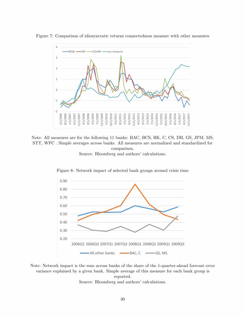
Figure 7: Comparison of idiosyncratic returns connectedness measure with other measures
‐2
‐1
0
1
2
3
4
3/1/20
068/1/20
061/1/20
076/1/20
0711
/1/200
74/1/20
089/1/20
082/1/20
097/1/20
0912
/1/200
95/1/20
1010
/1/201
03/1/20
118/1/20
111/1/20
126/1/20
1211
/1/201
24/1/20
139/1/20
132/1/20
147/1/20
1412
/1/201
45/1/20
1510
/1/201
53/1/20
168/1/20
161/1/20
176/1/20
1711
/1/201
7
SRISK DIP COVAR our measure
Note: All measures are for the following 11 banks: BAC, BCS, BK, C, CS, DB, GS, JPM, MS,STT, WFC . Simple averages across banks. All measures are normalized and standardized for
comparison.Source: Bloomberg and authors’ calculations.
Figure 8: Network impact of selected bank groups around crisis time
0.20
0.30
0.40
0.50
0.60
0.70
0.80
0.90
2006Q1 2006Q3 2007Q1 2007Q3 2008Q1 2008Q3 2009Q1 2009Q3
Impact
All other banks BAC, C GS, MS
Note: Network impact is the sum across banks of the share of the 1-quarter-ahead forecast errorvariance explained by a given bank. Simple average of this measure for each bank group is
reported.Source: Bloomberg and authors’ calculations.
30

Figure 9: ROA decomposition for Wells Fargo
−0.
006
−0.
004
−0.
002
0.00
00.
002
0.00
40.
006
ROAResidualFitted
2002
Q2
2002
Q4
2003
Q2
2003
Q4
2004
Q2
2004
Q4
2005
Q2
2005
Q4
2006
Q2
2006
Q4
2007
Q2
2007
Q4
2008
Q2
2008
Q4
2009
Q2
2009
Q4
2010
Q2
2010
Q4
2011
Q2
2011
Q4
2012
Q2
2012
Q4
2013
Q2
2013
Q4
2014
Q2
2014
Q4
2015
Q2
2015
Q4
2016
Q2
2016
Q4
2017
Q2
2017
Q4
Note: Reported are quarterly return on assets as well as fitted values and residuals from theMIDAS regression estimated for the full sample period as shown.
Source: Bloomberg and authors’ calculations.
31

Figure 10: R2 from MIDAS regression
BA
C
BB
T
BB
VA C
CM
A
HB
AN
JPM
KE
Y
MT
B
NT
RS
PN
C
ST
I
ST
T
US
B
WF
C
ZIO
N
00.
10.
20.
30.
40.
50.
60.
70.
80.
91
Source: Bloomberg and authors’ calculations.
Figure 11: Adjacency matrix for observed ROA component (last rolling window)
BAC BBT BBVA C CMA HBAN JPM KEY MTB NTRS PNC STI STT USB WFCBBT 0.70BBVA 0.08 0.45C 0.57 0.75 0.67CMA 0.51 0.79 0.43 0.79HBAN 0.32 0.04 0.06 0.31 0.28JPM 0.00 0.01 0.33 0.23 0.13 0.06KEY 0.43 0.63 0.29 0.77 0.78 0.22 0.00MTB 0.50 0.51 0.23 0.58 0.60 0.63 0.00 0.71NTRS 0.18 0.00 0.00 0.14 0.00 0.60 0.00 0.03 0.10PNC 0.81 0.71 0.17 0.68 0.55 0.29 0.09 0.49 0.46 0.20STI 0.55 0.24 0.00 0.09 0.08 0.30 0.00 0.34 0.61 0.08 0.21STT 0.54 0.20 0.00 0.26 0.29 0.21 0.00 0.29 0.21 0.25 0.36 0.13USB 0.77 0.73 0.33 0.63 0.62 0.40 0.00 0.56 0.72 0.13 0.51 0.57 0.41WFC 0.41 0.51 0.50 0.55 0.33 0.00 0.00 0.38 0.40 0.00 0.20 0.37 0.11 0.75ZION 0.56 0.40 0.29 0.58 0.69 0.72 0.02 0.57 0.69 0.23 0.45 0.32 0.55 0.56 0.10
Note: Reported are correlation coefficients (with negative numbers replaced with zeros) for thefitted values from ROA MIDAS regression. Correlations are computed for the last 16 quarters of
the sample.Source: Bloomberg and authors’ calculations.
32

Figure 12: Adjacency matrix for unobserved ROA component (last rolling window)
BAC BBT BBVA C CMA HBAN JPM KEY MTB NTRS PNC STI STT USB WFCBBT 0.40BBVA 0.12 0.21C 0.17 0.33 0.68CMA 0.38 0.12 0.18 0.24HBAN 0.29 0.10 0.06 0.23 0.73JPM 0.10 0.00 0.17 0.25 0.22 0.00KEY 0.39 0.55 0.16 0.60 0.43 0.46 0.14MTB 0.35 0.42 0.26 0.34 0.69 0.61 0.13 0.64NTRS 0.01 0.00 0.02 0.08 0.36 0.49 0.00 0.00 0.14PNC 0.18 0.30 0.00 0.36 0.00 0.37 0.00 0.67 0.20 0.00STI 0.32 0.44 0.00 0.01 0.55 0.35 0.00 0.54 0.64 0.00 0.24STT 0.27 0.59 0.00 0.00 0.26 0.46 0.00 0.41 0.41 0.00 0.29 0.51USB 0.34 0.59 0.00 0.41 0.17 0.39 0.00 0.80 0.31 0.00 0.83 0.53 0.63WFC 0.13 0.55 0.26 0.49 0.00 0.11 0.00 0.63 0.14 0.00 0.79 0.25 0.42 0.86ZION 0.44 0.53 0.14 0.20 0.65 0.59 0.00 0.41 0.49 0.00 0.10 0.50 0.69 0.47 0.25
Note: Reported are correlation coefficients (with negative numbers replaced with zeros) for theresiduals from ROA MIDAS regression. Correlations are computed for the last 16 quarters of the
sample.Source: Bloomberg and authors’ calculations.
33

Figure 13: Connectedness of the observed ROA component — four largest banks
02
46
810
BACCJPMWFC
2006
Q1
2006
Q3
2007
Q1
2007
Q3
2008
Q1
2008
Q3
2009
Q1
2009
Q3
2010
Q1
2010
Q3
2011
Q1
2011
Q3
2012
Q1
2012
Q3
2013
Q1
2013
Q3
2014
Q1
2014
Q3
2015
Q1
2015
Q3
2016
Q1
2016
Q3
2017
Q1
2017
Q3
Note: Reported are average correlation coefficients (with negative numbers replaced with zeros)for the fitted values from ROA MIDAS regression for each of the four banks with all other banks
in the network.Source: Bloomberg and authors’ calculations.
34

Figure 14: Connectedness of the unobserved ROA component — four largest banks
02
46
8
BACCJPMWFC
2006
Q1
2006
Q3
2007
Q1
2007
Q3
2008
Q1
2008
Q3
2009
Q1
2009
Q3
2010
Q1
2010
Q3
2011
Q1
2011
Q3
2012
Q1
2012
Q3
2013
Q1
2013
Q3
2014
Q1
2014
Q3
2015
Q1
2015
Q3
2016
Q1
2016
Q3
2017
Q1
2017
Q3
Note: Reported are average correlation coefficients (with negative numbers replaced with zeros)for the residuals from ROA MIDAS regression for each of the four banks with all other banks in
the network.Source: Bloomberg and authors’ calculations.
35

Figure 15: Network density for ROA and its decomposition
0.1
0.2
0.3
0.4
0.5
0.6
2006
Q1
2006
Q3
2007
Q1
2007
Q3
2008
Q1
2008
Q3
2009
Q1
2009
Q3
2010
Q1
2010
Q3
2011
Q1
2011
Q3
2012
Q1
2012
Q3
2013
Q1
2013
Q3
2014
Q1
2014
Q3
2015
Q1
2015
Q3
2016
Q1
2016
Q3
2017
Q1
2017
Q3
ResidualsFittedROA
Note: Reported are average correlation coefficients (with negative numbers replaced with zeros)for ROA as well as fitted values and residuals from ROA MIDAS regression.
Source: Bloomberg and authors’ calculations.
36

Figure 16: Connectedness between observed and unobserved ROA components
residualsfitted BAC BBT BBVA C CMA HBAN JPM KEY MTB NTRS PNC STI STT USB WFC ZION
BAC 0.00 0.00 0.00 0.00 0.00 0.00 0.45 0.00 0.00 0.16 0.00 0.00 0.00 0.00 0.00 0.00BBT 0.00 0.00 0.00 0.00 0.00 0.00 0.12 0.00 0.00 0.31 0.00 0.00 0.00 0.00 0.00 0.00BBVA 0.00 0.00 0.00 0.00 0.00 0.00 0.00 0.00 0.00 0.04 0.00 0.22 0.21 0.01 0.00 0.00C 0.00 0.00 0.00 0.00 0.00 0.00 0.00 0.00 0.00 0.05 0.00 0.00 0.00 0.00 0.00 0.00CMA 0.00 0.00 0.00 0.00 0.00 0.00 0.00 0.00 0.00 0.16 0.00 0.00 0.00 0.00 0.00 0.00HBAN 0.00 0.00 0.00 0.00 0.00 0.00 0.00 0.00 0.00 0.00 0.00 0.00 0.00 0.00 0.00 0.00JPM 0.00 0.26 0.00 0.00 0.02 0.03 0.00 0.00 0.00 0.11 0.00 0.34 0.58 0.18 0.03 0.19KEY 0.00 0.00 0.00 0.00 0.00 0.00 0.00 0.00 0.00 0.09 0.00 0.00 0.00 0.00 0.00 0.00MTB 0.00 0.00 0.00 0.00 0.00 0.00 0.05 0.00 0.00 0.04 0.00 0.00 0.00 0.00 0.00 0.00NTRS 0.01 0.34 0.00 0.00 0.00 0.00 0.24 0.00 0.00 0.00 0.00 0.00 0.00 0.00 0.00 0.00PNC 0.00 0.00 0.00 0.00 0.06 0.00 0.33 0.00 0.00 0.10 0.00 0.00 0.00 0.00 0.00 0.00STI 0.00 0.00 0.20 0.09 0.00 0.00 0.28 0.00 0.00 0.16 0.00 0.00 0.00 0.00 0.00 0.00STT 0.00 0.00 0.07 0.00 0.17 0.00 0.59 0.00 0.08 0.00 0.00 0.00 0.00 0.00 0.00 0.00USB 0.00 0.00 0.00 0.00 0.00 0.00 0.30 0.00 0.00 0.15 0.00 0.00 0.00 0.00 0.00 0.00WFC 0.00 0.00 0.00 0.00 0.00 0.04 0.06 0.00 0.00 0.36 0.00 0.00 0.00 0.00 0.00 0.00ZION 0.00 0.00 0.00 0.00 0.00 0.00 0.08 0.00 0.00 0.00 0.00 0.00 0.00 0.00 0.00 0.00
Note: Reported are correlation coefficients (with negative numbers replaced with zeros) betweenfitted values and residuals from ROA MIDAS regression.
Source: Bloomberg and authors’ calculations.
37

Figure 17: Density of the subcomponents of the network that includes both observed andunobserved components of ROA for each bank
0.0
0.1
0.2
0.3
0.4
0.5
0.6
2006
Q1
2006
Q3
2007
Q1
2007
Q3
2008
Q1
2008
Q3
2009
Q1
2009
Q3
2010
Q1
2010
Q3
2011
Q1
2011
Q3
2012
Q1
2012
Q3
2013
Q1
2013
Q3
2014
Q1
2014
Q3
2015
Q1
2015
Q3
2016
Q1
2016
Q3
2017
Q1
2017
Q3
ResidualsFittedResiduals & Fitted
Note: Reported are average correlation coefficients (with negative numbers replaced with zeros)for fitted values and residuals as well as between fitted values and residuals from ROA MIDAS
regression.Source: Bloomberg and authors’ calculations.
38

Figure A1. Coefficients from rolling CAPM regressions.

Figure A2. Measures of impact and vulnerability based on CAPM regression – 4 largest banks
Impact:
Vulnerability:
Figure A3. Coefficients MIDAS regression
Panel A. Across banks on quarterly variables with 2-s.e. bands
Panel B. Across banks and weekly lags