Embed Size (px)
Citation preview

HYDROLOGICAL PROCESSESHydrol Process (2012)Published online in Wiley Online Library(wileyonlinelibrarycom) DOI 101002hyp9459
Monitoring and modeling dissolved oxygen dynamics throughcontinuous longitudinal sampling a case study in Wen-Rui
Tang River Wenzhou China
Jun Li12 Huixia Liu1 Yancheng Li1 Kun Mei1 Randy Dahlgren12 and Minghua Zhang121 Wenzhou Medical College Zhejiang China
2 Dept of Land Air and Water Resources University of California Davis CA USA
CRes956E-m
Co
Abstract
Synoptic water sampling at a fixed site monitoring station provides only limited lsquosnap-shotsrsquo of the complex water qualitydynamics within a surface water system However water quality often changes rapidly in both spatial and temporal dimensionsespecially in highly polluted urban rivers In this study we designed and applied a continuous longitudinal sampling technique tomonitor the fine-scale spatial changes of water quality conditions assess water pollutant sources and determine the assimilativecapacity for biochemical oxygen demand (BOD) in an urban segment of the hypoxic Wen-Rui Tang River in eastern China Thecontinuous longitudinal sampling was capable of collecting dissolved oxygen (DO) data every 5 s yielding a ~11 m samplinginterval with a precision of 01 mg L1 The Streeter and Phelps BOD-DO model was used to calculate (1) the oxygenconsumption coefficient (K1) required for calibration of water quality models (2) BOD assimilative capacity and (3) BODsource and load identification In the 2014 m river segment sampled the oxygen consumption coefficient (K1) was 0428 d1
(20C) the total BOD discharge was 916 kg d1 and the BOD assimilative capacity was 382 kg d1 when the minimum DOlevel was set to 2 mg L1 In addition the longitudinal analysis identified eight major drainage outlets (BOD point sources)which were verified by field observations This new approach provides a simple cost-effective method of evaluating BOD-DOdynamics over large spatial areas with rapidly changing water quality conditions such as urban environments It represents amajor breakthrough in the development and application of water quality sampling techniques to obtain spatially distributed DOand BOD in real time Copyright copy 2012 John Wiley amp Sons Ltd
KEY WORDS water quality monitoring oxygen consumption coefficient dissolved oxygen hypoxia Streeter and Phelps modelassimilative capacity
Received 29 November 2011 Accepted 19 June 2012
INTRODUCTION
China currently faces severe urban water quality problemsThe fact that 90 of urban waterways are classified asheavily polluted (SEPA-China 2005) has raised greatconcerns about human and aquatic ecosystem health (Zhanget al 2010 Voss 2011) Monitoring water quality is thefirst step toward understanding the characteristics of waterpollution and for devising effective mitigation strategiesTraditional synoptic sampling at a fixed monitoring stationprovides only a lsquosnap-shotrsquo understanding of the complexspatial-temporal water quality dynamics occurring within asurface water system This complexity is especiallypronounced in river systems spanning urban and agricul-tural land uses where numerous point and non-point inputsoccur over relatively short distances Thus the singleconstant assimilative capacity coefficient (self-purificationcoefficient) obtained from such sampling does not accur-ately portray the biochemical oxygen demand-dissolvedoxygen (BOD-DO) dynamics for large surface water
orrespondence to Minghua Zhang Department of Land Air and Waterources University of California Davis One Shields Ave Davis CA16 USAail mhzhangucdavisedu
pyright copy 2012 John Wiley amp Sons Ltd
systems crossing urban and agricultural boundaries In factdirect quantification of the assimilative capacity of rivers isvery difficult to measure (Tase et al 1993)As early as 1925 scientists have modeled BOD-DO
dynamics in polluted surface waters Streeter and Phelps(1925) proposed the well-known StreeterndashPhelps (SPmodel) Oxygen Sag Formula to describe the oxygenbalance in streams Throughout the years researchersfurther improved and applied these equations to variousscenarios (Theriault 1927 Fair 1939 Thomas 1948 Li1962 1972 Camp 1963 Beck and Young 1976Gundelach and Castillo 1976 Thomann and Muumlller1987 Yu et al 1991 Adrian et al 1994 Jolankai1997) Despite the emergence of many complex waterquality models (eg QUAL2E Brown and Barnwell 1987WASP6 Wool et al 2001) describing DO dynamicsresulting from changes of BOD the SP model and itsmodifications still remain among those most widely used(Gotovtsev 2010) In the SP model the oxygen consump-tion coefficient (K1) represents the rate of O2 consumptiondue to oxidation of organic matter and other reducedsubstances (eg NH4
+ Fe2+ S2-) The reaeration coefficient(K2) represents the rate of O2 input to the river and isinfluence by flow rate water depth turbulence (mixing)water temperature and degree of water column oxygen
J LI ET AL
saturation There are other methods for calculating thesecoefficients such as the empirical formula used to calculateK2 in the EPD-RIV1water qualitymodel (Martin andWool2002) The oxygen consumption coefficient (K1) is animportant parameter for current riverine water qualitymodels such as EPD-RIV1 and QUAL2K (Chapra andPelletier 2003) The accuracy of water quality predictions iscritically dependent on the selected K1 value as it is theprimary driver describing oxygen consumption ratesHowever it is not possible to determine K1 from synopticwater quality sampling alone While BOD kinetics can bedetermined in the laboratory such procedures requiresubstantial resources and laboratory measures cannotaccount for the complexities of oxygen consumptionoccurring in the real-world river setting (eg sedimentoxygen demand and diel cycles)The Wen-Rui Tang River located in Wenzhou
Zhejiang province is one of the most polluted rivers inChina with many portions of the 1178 km of urbanwaterways being dead zones due to persistent hypoxiaThe pollution problem is compounded by the very lowgradient and diversion of upstream waters which result inlittle or no flow to flush the pollutants from the urbanriver system during dry periods Because of their spatialcomplexity synoptic sampling may not accurately depictthe distribution of the pollutants sources in this systemconfounding proper management decisions This riverremains highly polluted despite a substantial investmentby the local government in recent years to clean it upTo better inform future policy and management
decisions the objective of this study was to monitor therapid spatial changes of water quality using continuous
Figure 1 Map of Hualongqiao River showing location of study site HualongCoordinates of the river center is (2
Copyright copy 2012 John Wiley amp Sons Ltd
longitudinal water quality monitoring technology and tomodel BOD-DO dynamics These data are then used toidentify the lsquohiddenrsquo drainage outlets from whichpollutants flow into the river and to estimate the oxygenconsumption coefficient to spatially evaluate the pollutantloads along the course of the river These can bedetermined by the difference analysis of the SP modeland its related parameters In contrast to BOD valuesdetermined in the lab continuous longitudinal monitoringfor DO is easily achieved and inexpensive using currentwater quality sensor technology Thus the specific focusof this study was to calculate the spatial variability inoxygen consumption (K1) and reaeration (K2) coefficientsusing temperature DO and GPS coordinates derivedfrom the continuous longitudinal monitoring The mod-eling results also allow for quantification of the BODassimilative capacity and BOD source and load identifi-cation The results of this study provide importantinformation to guide water quality modeling BOD sourceidentification and numerical targets for BOD loadreductions to meet water quality standards
MATERIALS AND METHODS
The study site
The Wen-Rui Tang River watershed is located inWenzhou City Zhejiang China (Figure 1) The watershedhas an area of 740 km2 with a population of about 72million and land-use distribution consisting of 145 urban395 agriculture 15 wetlands 38 hilly forest and65 others The main stem of the Wen-Rui Tang River
qiao River is one branch of Wen-Rui Tang River in Wenzhou China The759rsquo2806N 12040rsquo5408E)
Hydrol Process (2012)
MONITORING AND MODELING DISSOLVED OXYGEN DYNAMICS IN SURFACE WATERS
spans 204 km in the urban area and flows through a networkof interconnecting urban waterways with a total length of1178 km The width of the urban portion of the Wen-RuiTang River is about 50 m on average varying from about13 to 150 m Due to direct discharge of large amounts ofdomestic industrial and agricultural wastewater into theriver the water quality of the river is severely impairedparticularly since the rapid economic development of the1980s Many of the urban waterways are considered deadzones due to persistent hypoxia (AsianInfo Services 2004)As a result in 2008 the water quality was classified asinferior Type V the lowest water quality classification inChina (Wenzhou State of the Environment 2008)In this study a tributary of the Wen-Rui Tang River the
Hualongqiao River was selected as a case study forcontinuous water quality monitoring and BOD-DO ana-lysis This river segment is located at the urbanndashagriculturalinterface It had a length of 2014 m an average width of537 m and average depth of 20 m (Figure 1) and a veryslow flow velocity of 45 m h1 at the time of the study inOctober 2009 The river banks were occupied by an oldone-story urban district on one side and a new residentialdistrict on the other Domestic sewage was dischargeddirectly into the river through rainwater runoff and a brokensewage collection network In addition several drainageoutlets entered the river below the water line and were noteasily visible from the surface
Sampling design
A YSI 6920 multi-parameter water quality monitoringsonde (YSI Yellow Springs Ohio USA) was used tomeasure temperature probe depth conductivity pH DOtotal ammonia nitrogen (NH4
+ + NH3) and turbidity in realtime DOwasmeasured with a YSI 6150 Optical DO sensorwith a precision of 01 mg L1 or 1 of the reading(whichever was greater) in the range of 0 to 20 mg L1A handheld GPS (Trimble GEO-XT2008 SunnyvaleCalifornia USA) was used to log the longitude and latitudecoordinates (05 m precision) for each of the YSI 6920sampling points The continuous longitudinal monitoring ofsurface water quality comprised five steps
1 Calibration of the YSI 6920 water quality sensorsimmediately prior to data collection with verification ofthe calibration at the end of data collection
2 Synchronization of the YSI 6920 and GEO-XT2008GPS clocks and setting of the YSI sampling interval to5 s equivalent to ~112 m between sampling points
3 Attachment of the YSI 6920 on a motor boat with theprobe submerged 01 m into the water column followedby collection of data as the boat moves at a uniformspeed (~806 km h1) along the center line of the river
4 Export of data from the YSI and GPS into a GISprogram after sampling
5 Integration of YSI water quality data with the longitudeand latitude for each data point
This process produces a continuous water qualitymonitoring database containing nine parameters (time
Copyright copy 2012 John Wiley amp Sons Ltd
temperature depth specific conductance pH DO totalammonia-N turbidity and GPS coordinates) A total of180 sample points were collected along the 2014 m riversegment within a 1 h time interval
GIS data source and Geodatabase design
Background GIS data were obtained from WenzhouDepartment of Planning and Wenzhou River AssessmentOffice The data included satellite images taken in 2004with a 05 m resolution the polygon water system ofWen-Rui Tang River the census data of the undergroundstorm water collection system (2004) and the sewagenetwork system (2004) of the city The GIS SuperMapDeskpro 2008 software developed by SuperMap SoftwareCo Ltd (Beijing China) was used in this study All thebasic geographical data were imported to the GIS platformwhich manages the data efficiently The coordinate systemwas then set as the Wenzhou City coordinate system basedon the Xirsquoan reference system 1980 (Xian-80) Whendealing with the field data one should first import thedatabase into GIS software to form a data attribute tablethen take the fields (longitude latitude) as the horizontaland vertical (x y) axes using a coordinate system to formpoint datasets based on the attribute table and finallyconvert the coordinate system to Xian-80
The analysis method of BOD-DO relationship
BOD-DO relationship model selection Streeter andPhelps (1925) were the first to systematically studyoxygen consumption and reaeration in streams Althoughtheir model was modified for publicly available waterquality models at various times the basic functions of theSP model stayed the same in these later modified modelsThe original BOD-DO relationship equations were usedfor deriving the BOD dynamics based on our monitoredDO values Therefore the capacity of a stream to oxidizesewage (ie organic matter and ammonia) depends uponits oxygen dynamics and can be described by the SPOxygen Sag Formula (Streeter and Phelps 1925) in thefollowing equations
D frac14 Cs C (1)
dD
dtfrac14 K1L K2D (2)
D frac14 K1L0K2-K1
e-K1t-e-K2t thorn D0 e-K2t (3)
Dc frac14 L0K1
K2e-K1tc (4)
tc frac14 1K2-K1
LNK2
K1
1K2-K1
K1D0
L0
(5)
Where D is the oxygen deficit (mg L1) which is afunction of Cs DO concentration at 100 saturation asa function of temperature salinity and atmospheric
Hydrol Process (2012)
J LI ET AL
pressure (mg L1) and C the DO concentration (mg L1) Lis the ultimate BOD (mg L1) while L0 is the initial BOD(mg L1) K1 is the oxygen consumption coefficient to thebase e (per day) K2 is the reaeration coefficient to the basee (per day) t is the time of travel as t= xv in which x is thedistance from the upstream L0 point (day) v is the velocity(mday) and (tc Dc) is the critical point in which the rate ofchange of DO equals zero during downstream transportIn the classical model of Streeter and Phelps K1 K2
and L0 can be computed using three data points ndash anypoint 1 (t1 D1) any point 2 (t2 D2) and the oxygencritical point (tc Dc) from the oxygen sag curve Howeverthe oxygen sag curve involves binary exponential equationswhich are very difficult to solve Therefore in order tocompute K1 without the BOD data some pragmaticapproaches were developedBlack and Phelps (1911) were the first to develop a
pragmatic approach for determining the waste-assimilativecapacity of a stream and their methodology was laterrefined and used by Velz (Lin 2001) This pragmaticapproachwas called theVelzReaerationCurve (Velz 1939)and calculates the biochemically consumed dissolvedoxygen (DOused) and dissolved oxygen absorbed from theatmosphere (DOrea) by the following two equations
DOusedfrac14 DOa-DOneteth THORNthornDOrea (6)
DOrea frac14 1 B0
100
R0
100
t
M
539Q DOseth THORN (7)
Where DOnet is the DO at the end of a reach DOa is theinitial DO at the beginning of a reach R0 is the percent ofthe saturated DO absorbed into the water column whenthe initial DO is at 100 percent deficit (DO= 0) B0 is theinitial DO in percent of saturationM is the mixing time inminutes DOs is the DO saturation load and t is the timeof travelAfter settingmanipulating the factors Y = (
PtP
DOused)13 and X=
Pt a linear fit formula may be derived
Y= SX+ b The results are K1 = 6Sb and L0 = b3K1 where
K1 is the oxygen consumption coefficient per day and L0 isthe initial BOD This pragmatic approach involvesestimating the waste assimilative capacity (f=K2K1) of awater body using five of the parameters which were directlymeasured by our continuous longitudinal monitoring (flowvolume velocity probe depth temperature and DO and the13-step approach summarized by Lin (2001) The parameterR0 is affected by many factors and requires manual lookupfrom several data sources Therefore this method was notsuitable for the computerized estimation of the relevantparameters (K1 L0) listed above
Method of data analysis The DO saturation values Csfor various water temperatures can be calculated using themethod of Elmore and Hayes (1960)
Cs frac14 14652 041022T thorn 00079910T2
0000077774T3(8)
Copyright copy 2012 John Wiley amp Sons Ltd
Because the Wen-Rui Tang River was a low-velocityriver (45 m h1) at the time of the study the reaerationcoefficient (K2) was estimated using the equationsdeveloped by OrsquoConnor and Dobbins (1958) where thereaeration coefficient (K2) is a function of the diffusivityof oxygen in addition to the riverrsquos average depth flowvelocity and temperature
K2 20Ceth THORN frac14 Dmueth THORN05d15
(9)
K2T frac14 1016T-20 K2 20Ceth THORN (10)
K1T frac14 1047T-20 K1 20Ceth THORN (11)
Where Dm is diffusivity of oxygen in water d isaverage depth u is flow velocity and T is temperature
Differential analysis of the SP model According to theSP Oxygen Sag Formula the following three equationscan be derived from each other and used interchangeably
dC
dtfrac14 K1L K2 Cs Ceth THORN (12)
The difference approximation is
ΔCΔt
frac14 K1L K2 Cs Ceth THORN (13)
or
K1Ln frac14 K2Cs nthorn1 thorn Cs n
2 Cnthorn1 thorn Cn
2
Cnthorn1 Cn
tnthorn1 tn
(14)
Where n is the first monitoring point Because K2 isassumed to be a known constant we can derive a seriesof K1Ln values According to the definition of K1 (dL dt =K1L) K1Ln is the BOD oxygen consumption rate forthe first sampling point (n)
Calculation of K1 If we collect data at uniformlyspaced points in the river we can use t= t0 + nΔt and thefollowing equation
Ln frac14 L0e-K1t frac14 L0e
-K1 t0 e-K1Δt n
(15)
In general K1 (to the base e) is less than 1 When thedistance of the continuous longitudinal sampling in theriver is short enough to make K1Δtlt 01 there will be astrong linear relationship between Ln and n or K1Ln and nAs K1Δt decreases in value the linear correlation increasesThrough this linear relationship we can re-calculate Lrsquo1and Ln
rsquo and use them to calculate K1 as shown in thefollowing equation
Hydrol Process (2012)
MONITORING AND MODELING DISSOLVED OXYGEN DYNAMICS IN SURFACE WATERS
K1 frac14 1n-1eth THORNΔt LN
L01
L0n
frac14 1n-1eth THORNΔt LN
K1L01
K1L0n
(16)
Selection of DO data meeting the SP model assumptionsand for point source assessment The SP model is a one-dimensional steady-state model for DO-BOD relation-ships In theory it requires an instantaneous mixing of thesewage with the river water throughout the river crosssection In reality near the sewage outlet this isimpossible Therefore we must identify the DO datafrom the continuous monitoring data which are suitablefor use in the SP model Ideally these data should befrom the section where the sewage has already beenuniformly mixed with the water column and indicated bya good linear relationship between K1Ln and n At bothends of the longitudinal DO data set the DO data deviateappreciably from this linear relationship so these datawere discardedWe were also able to assess locations of point source
BOD inputs within the river reach In the longitudinal DOdata set the critical point is a key data parameter in whichthe rate of change for DO is zero and the key data (Cc tc)point was used to compute the initial BOD (L0) using thefollowing formula
L0 frac14 Cs-Cceth THORN K2
K1 eK1tc (17)
The initial BOD (L0) is composed of two parts one partof the discharge stems from the sewage outlet Loutletwhile the other part originates from BOD imported fromupstream sewage L0rsquo (Loutlet = L0 - L0rsquo)
Figure 2 Dissolved Oxygen (DO) variations in Hualongqiao River fromupstream to downstream DO is percent of saturation The light blue showsthe river width in the sampled segment similarly as shown in Figure 3 and 4
RESULTS
Table I provides an example of the continuous longitu-dinal data and its structure Among the total of 180 datapoints collected along the 2014 m river segment (~112 m
Table I Longitudinal continuous
Temp CondTime lat Long C S cm1
141734 1206705 279869 253 025141739 1206706 279870 253 025141744 1206707 279870 253 025141749 1206708 279871 252 025 143249 1206873 279933 257 025143254 1206875 279934 257 025143334 1206883 279939 254 026143339 1206884 279940 255 026
Copyright copy 2012 John Wiley amp Sons Ltd
between sampling points) there were 36 data pointswhich lacked GPS coordinates because the GPS receivercould not receive satellite signals when the boat navigatedunder bridges These missing GPS coordinates wereinterpolated between measured GPS points assuming auniform boat speed of 806 km h1
Trend of dissolved oxygen and identification of the hiddendrainage outlets
The average DO concentration was 218 of saturation(which is equivalent to 175 mg L1) and ranged from 94(076 mg L1) to 364 (29 mg L1) (Figure 2) Averagetotal ammonia nitrogen concentration was 725 mg L1ranging from 593 to 816 mg L1 (Figure 3) with manypeaks within the river segment Water temperaturedisplayed about a 1C variation along the river segmentwith an average temperature of 256C (Figure 4) The peaksof temperature ammonia and DO occurred at a distance of700 m where a tributary joins the Hualongqiao River(Figures 2ndash4)Changes in DO concentrations along the river segment
are shown in Figure 5 According to the SP OxygenSag Curve Figure 5 displays eight positive peaks in theDO curve The rate of change ie ΔDOΔL was verifiedto correspond to the maximum BOD concentrations asshown by the red solid line in Figure 5 which are relatedto the locations of eight sewage drainage outlets (pointsources) The minimum values in the DO curve (when
water quality monitoring data
Probe Depth Ammonium-N Turb DOm pH mg L1 NTU
01 671 73 236 12301 670 75 225 11301 670 77 214 10601 670 78 203 99
01 676 71 64 25001 676 69 63 25801 675 74 71 18901 675 74 70 204
Hydrol Process (2012)
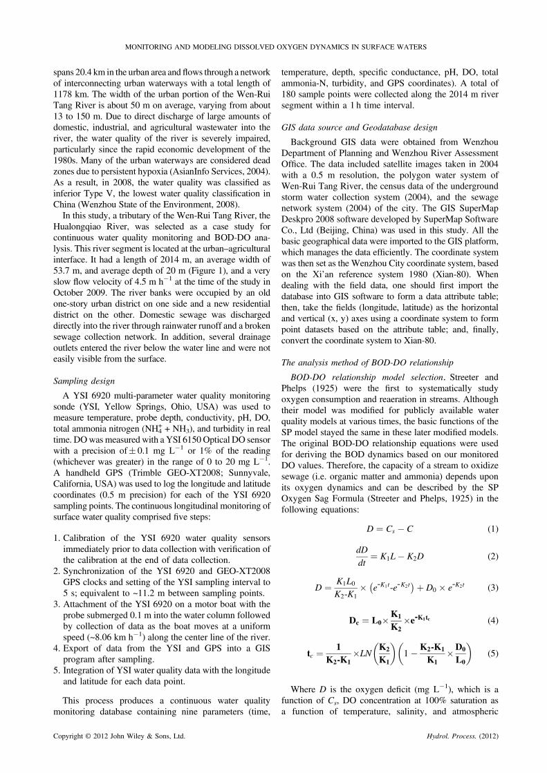
Figure 3 Ammonium-N variations in Hualongqiao River from upstreamto downstream
Figure 4 Temperature variations in Hualongqiao River from upstream todownstream
Figure 5 DO variations and DO rate of variations in Hualongqiao Riverfrom upstream to downstream The symbols from A1 to A8 are thepositions of the sewage outlets based on the analysis of DO peaks andverified in the field The DO rates of variations are only shown between
the two sewage outlets
J LI ET AL
ΔDOΔL= 0) are identified as the critical points atwhich DO rate of change is equal to zero The SPOxygen Sag Curve will show a single maximum andminimum peak in the trend of DO if there is only onewastewater outlet in a river However eight such twinpeaks (maxima and minima) were observed in Figure 5which correspond to eight major sewage outlets in theriver segment The locations of the outlets designated A1through A8 in Figure 5 were verified by the fieldinvestigation This revelation shows that the continuous
Copyright copy 2012 John Wiley amp Sons Ltd
longitudinal sampling for DO can accurately identify thehidden sewage outlets under the water surface
Calculation of K1 the oxygen consumption coefficient
In general K1 to the base e is considered to be aconstant Therefore K1 was calculated using the DO datain the A4ndashA5 segment shown in Figure 5 This riversegment contains more monitoring points resulting in asmooth curve that indicates that there are no majorwastewater sources in this segment The DO data for theA4ndashA5 segment and related parameters used to calculateK1 are listed in Table IIIn the case study Δt = 01147 and K1lt 08 so
K1Δtlt 01 Since the value of K1Δt was much smallerthan the threshold of 095 (as defined in section 244) astrong linear relationship between K1Ln and n wasexpected Figure 6 shows the linear relationship betweenK1Ln and n using the DO data from the A4ndashA5 riversegment Based on Equation (17) oxygen consumptioncoefficients (K1) of 0552 d1 (25C) and 0428 d1
(20C) were obtainedWhen the Velz Reaeration Curve was used to
independently calculate K1 results were b = 0193S = 0017 and K1 = 6sb = 0528 d1 The results of thetwo K1 estimation approaches using our derived approachand the Velz Reaeration Curve were similar (0552 vs0528 d1 25C) supporting the validity of using our newapproach in calculating K1
Calculation of L0 and assessment of point source pollution
The calculated BOD discharge loads from wastewateroutlets A1 to A8 are listed in Table III Outlets A5 andA7 released the largest amount of BOD at 226 and 234 kgd1 respectively followed by the outlets A1 and A4 at104 and 121 kg d1 respectively while outlets A2 A3A6 and A8 released BOD loads of less than 100 kg d1
(Table III) The sum of BOD loads from the eight outletsindicates the total amount of BOD discharged into theriver segment examined in this study was 916 kg d1
Computation of self-purification capacity
The BOD assimilative capacity (K2K1) ie self-purification capacity was calculated based on designatedminimum DO values which correspond to the criticalpoints of the oxygen sag curve We assumed that thesewage outlets in the river were upstream and thatthe amount of the initial DO was equal to the amountof DO at saturation or D0 = 0 Following the analysis ofinferences in Section 244 286 days (tc) wererequired for DO to change from the highest value tothe lowest valueThe minimum dissolved oxygen (Dc) of the river was set
to four water quality standard values ranging from 2ndash6 mgL1 which correspond to four water quality classificationgrades in China The results of the computation for BODload capacity ranged from 129 kg d1 to maintain the 6 mgL1 DO minimum standard to 382 kg d1 to maintain the2 mg L1 DO minimum standard (Table IV)
Hydrol Process (2012)
Table II Calculation of K1 using the DO data in A4ndashA5 segment
Length Temp C Cs Mean Cs Mean C ΔtNo meter C mg L1 mg L1 mg L1 mg L1 days ΔC K2 K1L n
74 00 263 290 797 0 020775 128 258 265 806 801 278 0118 025 0205 31976 127 256 232 809 807 249 0118 033 0204 39477 126 255 208 810 809 22 0117 024 0204 32678 126 255 195 810 810 202 0117 013 0204 236 179 125 255 187 810 810 191 0116 008 0204 195 280 124 255 180 810 810 184 0115 007 0204 189 381 124 255 175 811 810 178 0115 005 0204 174 482 124 254 171 811 811 173 0115 004 0204 165 583 123 254 166 811 811 169 0113 005 0204 175 684 123 254 163 811 811 165 0114 003 0204 158 785 122 254 161 811 811 162 0113 002 0204 150 886 122 255 162 811 811 162 0113 001 0204 124 987 123 255 164 810 810 163 0114 002 0204 115 1088 119 255 166 810 810 165 0110 002 0204 114 1189 123 255 167 810 810 167 0114 001 0204 123 1290 125 255 170 810 810 169 0116 003 0204 105 1391 126 255 173 810 810 172 0117 003 0204 105 1492 122 255 177 810 810 175 0113 004 0204 094 1593 121 255 183 810 810 18 0112 006 0204 075 1694 122 255 187 810 810 185 0113 004 0204 092
Notes Velocity = 000125ms Depth = 185m
Figure 6 The analysis of the linear relationship between K1Ln and n
Table III Assessment of point source pollution
L0 L00 Loutfall Flow Q LoutfallStation mg L1 mg L1 mg L1 m3 d1 kg d1
A1 30 00 30 35 191 104A2 33 20 13 35 191 46A3 25 082 17 35 191 59A4 49 14 34 35 191 120A5 78 14 64 35 191 226A6 28 08 20 35 191 69A7 79 12 66 35 191 234A8 35 19 17 35 191 58
Notes L0 is the initial BOD Lrsquo0 is the BOD from upstream Loutfall is thedischarge of the sewage outfall
Table IV Computation of self-purification capacity
DO standards Self-purification capacityWater quality types mgL mgL kgday
II 6 37 129III 5 55 192IV 3 90 318V 2 11 381
Notes Flow= 0407 m3 s1 Average temperature = 2552 C K2 = 0204d1 K1 = 0552 d1
Figure 7 Observed DO data and model prediction curve in HualongqiaoRiver
MONITORING AND MODELING DISSOLVED OXYGEN DYNAMICS IN SURFACE WATERS
Figure 7 shows that the observed DO (black line) washighly correlated (r= 068) with the model-generated DO(red line) concentrations along the river segment Thisanalysis indicated that the model reasonably predicted theDO values for the river segment in this study Since theSP model requires an unrealistic instantaneous mixing of
Copyright copy 2012 John Wiley amp Sons Ltd
the wastewater with the river water it is not surprisingthat the two large peaks for predicted DO do not matchwell with the observed DO
Hydrol Process (2012)
J LI ET AL
DISCUSSION
The calculated oxygen consumption coefficient (K1)varies with temperature as indicated by the value of0552 d1 at 256C (ambient) and 0428 d1 normalizedfor 20C The greater the K1 value the faster oxygen isbeing consumed Thus the relatively high K1 value in theHualongqiao River indicates that oxygen consumption israpid and that inputs of oxygen demanding substances arevery severe in this river segment This is consistent withthe water quality classification of inferior Type V (lt2 mgL1 O2) that is common throughout Wenzhou Citywaterways (Wenzhou State of the Environment 2008)The calculated BOD discharged into the river segment916 kg d1 was considerably higher than theBOD receivingload capacity for type V water quality of 381 kg d1 basedon the 2 mg L1 DO minimum Thus BOD discharge intothe river segment would need to be reduced by 535 kg d1 tomeet the minimumwater quality standard DO concentrationof 2 mg L1 This specific reduction target provides a usefulreference point for the municipal government to properlydevise water management decisionsThis theoretical analysis has practical implications for
water quality assessment By showing that the K1 andBOD assimilative capacity may be computed using onlyDO data collected in a rigorous longitudinal fashion thismethod obtains real-time water quality information usingfar less resources than traditional laboratory methodsAlthough the Velz Reaeration Curve (Velz 1939 Lin2001) also calculates an oxygen consumption coefficient(K1) using only DO data (K1 was 0528 d1 using theVelz Reaeration Curve) it is far more cumbersome ifcontinuous longitudinal DO data are not availableThe new monitoring and calculation approach analyzed
and demonstrated in this study is direct simple and suitablefor automated computer processing for water qualityassessment The ability to rapidly collect densely packedDO concentration measurements with high precision usingthe continuous longitudinal monitoring technology makesthis new approach possible in real times The oxygenconsumption coefficient (K1) is a critical parameter drivingoxygen dynamics in many water quality models such as theEPD-RIV1 and QUAL2K developed by the US Environ-mental ProtectionAgency However with the application ofthese water quality models parameter calibration has been akey problem that is difficult to resolve with confidence Thedata collection and analysis methods proposed in this studycan be used to spatially determine the critical oxygenconsumption coefficient (K1) for a given watershed Thisapproach is especially useful in highly polluted riverswhich are common in many rapidly developing countriesThe essence of this approach is the use of dense DO
sampling to obtain the rate of change for DO concentrationsallowing the use ofΔCΔt instead of dCdt in the differentialequations used to describe the BOD-DO relationships Thisgreatly reduces the difficulty of solving the differentialequations Dense sampling requires data collectionmethods that are convenient fast reliable and low costThe continuous longitudinal water quality monitoring using
Copyright copy 2012 John Wiley amp Sons Ltd
sondes with multiple sensors meets these requirementsHowever to facilitate subsequent data analysis and optimizemodel results some additional requirements for samplingfrequency and uniform sampling distance by continuouslongitudinal monitoring must be met
Data quality and its influence
A sensitivity analysis examining experimental variabilityin water quality data acquired by the YSI sonde in this studyindicates low (lt2) variability in predicted parametersbased on the expected sonde variability The YSI 6150Optical DO sensor uses a fast interception system formeasuring DO This type of fast interception system uses aClark sensor to measure the return of electrons diffusedthrough a Teflon membrane The accuracy of DO measure-ments is influenced by temperature and the flow of the watersystem around the sonde Temperature was automaticallycorrected using the measured water temperatures Basedon the YSI userrsquos manual DO readings will be decreased by2ndash3 at the speed of our boat compared to DO readingsin still water Considering this difference we recalculatethe K1 as 0554 ~ 0556 d
1 (25C) compared to K1 = 0552d1 (25C) for non-velocity corrected values Thesedifferences result in K1 value differences 04ndash07 lowerand L0 values 07ndash1 higher Since all DO measurementswere taken at a constant boat travel velocity all of ourmeasurements are internally consistent
Sampling frequency requirements
The continuous longitudinal monitoring of rivers isactually a kind of digitization of the continuous DO dataTherefore in accordance with the requirements of theSamplingTheorem (Shannon 1949) the sampling frequencymust be greater than twice the highest frequency of the analogsignals Under this condition the sampling results may befully representative of the original analog signal For bestresults with respect to real-world sampling the samplingfrequency should be set as three to five times the highestsignal frequency The SP model requires an instantaneousmixing of the wastewater with the river water to produce avalid sampling point but these mixing conditions near thesewage outlets are not possible to fully achieve Consideringthese factors we set the sampling frequency at eight timeshigher than the signal frequency In the river segmentexamined the minimum distance between the identifiedsewage outlets was 85 m therefore the distance betweenmonitoring points was set to approximately 11 m (858 m)
Limitation and applicability
The application of continuous longitudinal water qualitysampling data provides a theoretical basis for obtaining theoxygen consumption coefficient which is otherwise difficultto acquire however there are some limitations One of theconditions required to maintain the linear relationshipbetween K1L and n is a uniform Δt If we assume that thewater flow rate is constant this is accomplished byuniformly spaced sampling times (5 s interval in this study)The water quality sonde is fixed on the boat which must
Hydrol Process (2012)
MONITORING AND MODELING DISSOLVED OXYGEN DYNAMICS IN SURFACE WATERS
move at a uniform speed to meet the uniform samplingdistance requirement The continuous longitudinal monitor-ing method presented here is also one dimensional so themonitoring boat must move along the center line of the riverto achieve optimum data collection In addition due to thespecific conditions of the river segment examined twocomplicated terms in the equations were considerednegligible Future research may explore the non-linearrelationships between the K1L and n as well as expandingthe analysis to two- or three-dimensional calculations of theessential water quality parameters for broader application tosustainable water resource management
CONCLUSION
This study used a branch of the Wen-Rui Tang River asa case study to demonstrate the efficacy of using alongitudinal continuous water quality monitoring method-ology to model BOD-DO dynamics in a hypoxic urbanriver The results indicated that continuous longitudinalmonitoring of temperature and DO is a powerful approachfor quantifying several BOD-DO parameters This methodallows direct computation of the oxygen consumptioncoefficient (K1) BOD assimilative capacity BOD pointsource locations and total BOD loads discharged into theriver segment of interest With these values we are able tobetter evaluate changes in water quality and chart thecontinuous temporal and spatial distributions of BOD-DOdynamics in complex urban waterways This approach canbe applied to any other complex urban waterways with slowflow movement for water quality assessment
ACKNOWLEDGEMENTS
This research was fully funded by Science and TechnologyDepartment of Zhejiang Province China through ProjectNo 2008C03009 Wenzhou River Assessment Officethrough Project No 20082780125 Authors wish to thankDr Michael Grieneisen for improving the English in thepaper Authors would also like to thank the editor andthe anonymous reviewers for constructive comments toimprove the paper
REFERENCES
Adrian DD Yu FX Barbe D 1994 Water quality modeling for asinusoidally varying waste discharge concentrations Water Research28 1167ndash1174
AsianInfo Services 2004 Wenzhou treats river with biological remediationtechnology httpwwwallbusinesscomenvironment-natural-resourcespollution7687802ndash1
Beck MB Young PC 1976 Systematic identification of DO-BOD modelstructure Journal of the Environmental Engineering Division ASCE102 902ndash927
Black WM Phelps EB 1911 Location of sewer outlets and discharge ofsewage in New York Harbor New York City Board of Estimate andApportionment March 23 1911
Brown LC Barnwell TO 1987 The enhanced stream water qualitymodels QUAL2E and QUAL2E-UNCAS documentation and user
Copyright copy 2012 John Wiley amp Sons Ltd
manual Environmental Research Laboratory US EPA WashingtonDC
Camp TR 1963 First expanded BOD-DO model In Basic River WaterQuality Models (IHP-V Project 81) Jolankai DG (ed) UNESCOPublications Paris 27ndash29
Chapra SC Pelletier GJ 2003 QUAL2K A Modeling Framework forSimulating River and Stream Water Quality Documentation and UsersManual [J] Civil and Environmental Engineering Dept TuftsUniversity Medford
Elmore HL Hayes TW 1960 Solubility of atmospheric oxygen inwater Journal of the Sanitation Engineering Division ASCE 8641ndash53
Fair GM 1939 The dissolved oxygen sagmdashan analysis Sewage WorksJournal 11 445ndash461
Gotovtsev AV 2010 Modification of the StreeterndashPhelps system withthe aim to account for the feedback between dissolved oxygenconcentration and organic matter oxidation rate Water Resources 37245ndash251
Gundelach JM Castillo JE 1976 Natural stream purification underanaerobic conditions Journal Water Pollution Control Federation 481753ndash1758
Jolankai G 1997 Basic river water quality models Technical Documentsin Hydrology no 13 IHP-V UNESCO Paris 50
Li WH 1962 Unsteady dissolved-oxygen sag in a stream Journal of theEnvironmental Engineering Division ASCE 88 75ndash85
Li WH 1972 Effects of dispersion on DO-SAG in uniform flow Journalof the Environmental Engineering Division ASCE 98 169ndash182
Lin SD 2001 Water and wastewater calculation manual McGrow-HillCompanies USA 854
Martin JL Wool TA 2002 A dynamic one-dimensional modelofhydrodynamics and water quality (EPD-RIV1)version 10ModelDocumentation and User Manual Georgia Environmental ProtectionDivision Atlanta GA
OrsquoConnor DJ Dobbins WE 1958 The mechanism of reaeration in naturalstreams Journal of the Environmental Engineering Division ASCE123 641ndash684
Shannon CE 1949 Communication in the presence of noise ProceedingsInstitute of Radio Engineers 37 10ndash21
State Environmental Protection Administration of China 2005 ChinaUrban Environmental Management 200562 P12
Streeter HW Phelps EB 1925 A Study of the pollution and naturalpurification of the Ohio river III Factors concerned in the phenomenaof oxidation and reaeration Public Health Bulletin no 146 Reprintedby US Department of Health Education and Welfare Public HealthService 1958 ISBN B001BP4GZI httpdspaceudeledu8080dspacebitstreamhandle197161590C26EE148pdfsequence=2
Tase N Arai H Suzumura T 1993 Use of 15N isotope as a natural tracerfor evaluating self-purification in the Tamagawa Jousui ChannelInternational Association of Hydrological Sciences Publications 215225ndash231
Theriault EJ 1927 The dissolved oxygen demand of polluted watersPublic Health Bulletin no 173 US Public Health Service WashingtonDC 189
Thomann RV Muumlller JA 1987 Principles of Surface Water QualityModelling and Control Harper amp Row New York
Thomas HA 1948 Pollution load capacity of streams Water amp SewageWorks 95 409ndash413
Velz CJ 1939 Deoxygenation and reoxygenation Transactions of theAmerican Society of Civil Engineers 104 560ndash572
Voss S 2011 Industrial pollution kills hundreds along the Huai RiverBasin in China httpwwwstephenvosscomstoriesChinaWaterPollu-tionstoryhtml Available October 15 2011
Wenzhou State of the Environment 2008 The State of Environment inWenzhou in 2008 httpwwwouhaigovcnart200965art_2175_21881html
Wool TA Ambrose RB Martin JL Comer EA 2001 US EnvironmentalProtection AgencyndashRegion Atlanta GA Environmental ResearchLaboratory Athens GA USACE ndash Waterways Experiment StationVicksburg MS Tetra Tech Inc Atlanta GA
Yu FX Adrian DD Singh P 1991 Modeling river quality by thesuperposition method Journal of Environmental Systems 20 1ndash16
Zhang J Mauzerall DL Zhu T Liang S Ezzati M Remais JV 2010Environmental health in China Progress toward clean air and safewater Lancet 375 1110ndash1119
Hydrol Process (2012)

J LI ET AL
saturation There are other methods for calculating thesecoefficients such as the empirical formula used to calculateK2 in the EPD-RIV1water qualitymodel (Martin andWool2002) The oxygen consumption coefficient (K1) is animportant parameter for current riverine water qualitymodels such as EPD-RIV1 and QUAL2K (Chapra andPelletier 2003) The accuracy of water quality predictions iscritically dependent on the selected K1 value as it is theprimary driver describing oxygen consumption ratesHowever it is not possible to determine K1 from synopticwater quality sampling alone While BOD kinetics can bedetermined in the laboratory such procedures requiresubstantial resources and laboratory measures cannotaccount for the complexities of oxygen consumptionoccurring in the real-world river setting (eg sedimentoxygen demand and diel cycles)The Wen-Rui Tang River located in Wenzhou
Zhejiang province is one of the most polluted rivers inChina with many portions of the 1178 km of urbanwaterways being dead zones due to persistent hypoxiaThe pollution problem is compounded by the very lowgradient and diversion of upstream waters which result inlittle or no flow to flush the pollutants from the urbanriver system during dry periods Because of their spatialcomplexity synoptic sampling may not accurately depictthe distribution of the pollutants sources in this systemconfounding proper management decisions This riverremains highly polluted despite a substantial investmentby the local government in recent years to clean it upTo better inform future policy and management
decisions the objective of this study was to monitor therapid spatial changes of water quality using continuous
Figure 1 Map of Hualongqiao River showing location of study site HualongCoordinates of the river center is (2
Copyright copy 2012 John Wiley amp Sons Ltd
longitudinal water quality monitoring technology and tomodel BOD-DO dynamics These data are then used toidentify the lsquohiddenrsquo drainage outlets from whichpollutants flow into the river and to estimate the oxygenconsumption coefficient to spatially evaluate the pollutantloads along the course of the river These can bedetermined by the difference analysis of the SP modeland its related parameters In contrast to BOD valuesdetermined in the lab continuous longitudinal monitoringfor DO is easily achieved and inexpensive using currentwater quality sensor technology Thus the specific focusof this study was to calculate the spatial variability inoxygen consumption (K1) and reaeration (K2) coefficientsusing temperature DO and GPS coordinates derivedfrom the continuous longitudinal monitoring The mod-eling results also allow for quantification of the BODassimilative capacity and BOD source and load identifi-cation The results of this study provide importantinformation to guide water quality modeling BOD sourceidentification and numerical targets for BOD loadreductions to meet water quality standards
MATERIALS AND METHODS
The study site
The Wen-Rui Tang River watershed is located inWenzhou City Zhejiang China (Figure 1) The watershedhas an area of 740 km2 with a population of about 72million and land-use distribution consisting of 145 urban395 agriculture 15 wetlands 38 hilly forest and65 others The main stem of the Wen-Rui Tang River
qiao River is one branch of Wen-Rui Tang River in Wenzhou China The759rsquo2806N 12040rsquo5408E)
Hydrol Process (2012)
MONITORING AND MODELING DISSOLVED OXYGEN DYNAMICS IN SURFACE WATERS
spans 204 km in the urban area and flows through a networkof interconnecting urban waterways with a total length of1178 km The width of the urban portion of the Wen-RuiTang River is about 50 m on average varying from about13 to 150 m Due to direct discharge of large amounts ofdomestic industrial and agricultural wastewater into theriver the water quality of the river is severely impairedparticularly since the rapid economic development of the1980s Many of the urban waterways are considered deadzones due to persistent hypoxia (AsianInfo Services 2004)As a result in 2008 the water quality was classified asinferior Type V the lowest water quality classification inChina (Wenzhou State of the Environment 2008)In this study a tributary of the Wen-Rui Tang River the
Hualongqiao River was selected as a case study forcontinuous water quality monitoring and BOD-DO ana-lysis This river segment is located at the urbanndashagriculturalinterface It had a length of 2014 m an average width of537 m and average depth of 20 m (Figure 1) and a veryslow flow velocity of 45 m h1 at the time of the study inOctober 2009 The river banks were occupied by an oldone-story urban district on one side and a new residentialdistrict on the other Domestic sewage was dischargeddirectly into the river through rainwater runoff and a brokensewage collection network In addition several drainageoutlets entered the river below the water line and were noteasily visible from the surface
Sampling design
A YSI 6920 multi-parameter water quality monitoringsonde (YSI Yellow Springs Ohio USA) was used tomeasure temperature probe depth conductivity pH DOtotal ammonia nitrogen (NH4
+ + NH3) and turbidity in realtime DOwasmeasured with a YSI 6150 Optical DO sensorwith a precision of 01 mg L1 or 1 of the reading(whichever was greater) in the range of 0 to 20 mg L1A handheld GPS (Trimble GEO-XT2008 SunnyvaleCalifornia USA) was used to log the longitude and latitudecoordinates (05 m precision) for each of the YSI 6920sampling points The continuous longitudinal monitoring ofsurface water quality comprised five steps
1 Calibration of the YSI 6920 water quality sensorsimmediately prior to data collection with verification ofthe calibration at the end of data collection
2 Synchronization of the YSI 6920 and GEO-XT2008GPS clocks and setting of the YSI sampling interval to5 s equivalent to ~112 m between sampling points
3 Attachment of the YSI 6920 on a motor boat with theprobe submerged 01 m into the water column followedby collection of data as the boat moves at a uniformspeed (~806 km h1) along the center line of the river
4 Export of data from the YSI and GPS into a GISprogram after sampling
5 Integration of YSI water quality data with the longitudeand latitude for each data point
This process produces a continuous water qualitymonitoring database containing nine parameters (time
Copyright copy 2012 John Wiley amp Sons Ltd
temperature depth specific conductance pH DO totalammonia-N turbidity and GPS coordinates) A total of180 sample points were collected along the 2014 m riversegment within a 1 h time interval
GIS data source and Geodatabase design
Background GIS data were obtained from WenzhouDepartment of Planning and Wenzhou River AssessmentOffice The data included satellite images taken in 2004with a 05 m resolution the polygon water system ofWen-Rui Tang River the census data of the undergroundstorm water collection system (2004) and the sewagenetwork system (2004) of the city The GIS SuperMapDeskpro 2008 software developed by SuperMap SoftwareCo Ltd (Beijing China) was used in this study All thebasic geographical data were imported to the GIS platformwhich manages the data efficiently The coordinate systemwas then set as the Wenzhou City coordinate system basedon the Xirsquoan reference system 1980 (Xian-80) Whendealing with the field data one should first import thedatabase into GIS software to form a data attribute tablethen take the fields (longitude latitude) as the horizontaland vertical (x y) axes using a coordinate system to formpoint datasets based on the attribute table and finallyconvert the coordinate system to Xian-80
The analysis method of BOD-DO relationship
BOD-DO relationship model selection Streeter andPhelps (1925) were the first to systematically studyoxygen consumption and reaeration in streams Althoughtheir model was modified for publicly available waterquality models at various times the basic functions of theSP model stayed the same in these later modified modelsThe original BOD-DO relationship equations were usedfor deriving the BOD dynamics based on our monitoredDO values Therefore the capacity of a stream to oxidizesewage (ie organic matter and ammonia) depends uponits oxygen dynamics and can be described by the SPOxygen Sag Formula (Streeter and Phelps 1925) in thefollowing equations
D frac14 Cs C (1)
dD
dtfrac14 K1L K2D (2)
D frac14 K1L0K2-K1
e-K1t-e-K2t thorn D0 e-K2t (3)
Dc frac14 L0K1
K2e-K1tc (4)
tc frac14 1K2-K1
LNK2
K1
1K2-K1
K1D0
L0
(5)
Where D is the oxygen deficit (mg L1) which is afunction of Cs DO concentration at 100 saturation asa function of temperature salinity and atmospheric
Hydrol Process (2012)
J LI ET AL
pressure (mg L1) and C the DO concentration (mg L1) Lis the ultimate BOD (mg L1) while L0 is the initial BOD(mg L1) K1 is the oxygen consumption coefficient to thebase e (per day) K2 is the reaeration coefficient to the basee (per day) t is the time of travel as t= xv in which x is thedistance from the upstream L0 point (day) v is the velocity(mday) and (tc Dc) is the critical point in which the rate ofchange of DO equals zero during downstream transportIn the classical model of Streeter and Phelps K1 K2
and L0 can be computed using three data points ndash anypoint 1 (t1 D1) any point 2 (t2 D2) and the oxygencritical point (tc Dc) from the oxygen sag curve Howeverthe oxygen sag curve involves binary exponential equationswhich are very difficult to solve Therefore in order tocompute K1 without the BOD data some pragmaticapproaches were developedBlack and Phelps (1911) were the first to develop a
pragmatic approach for determining the waste-assimilativecapacity of a stream and their methodology was laterrefined and used by Velz (Lin 2001) This pragmaticapproachwas called theVelzReaerationCurve (Velz 1939)and calculates the biochemically consumed dissolvedoxygen (DOused) and dissolved oxygen absorbed from theatmosphere (DOrea) by the following two equations
DOusedfrac14 DOa-DOneteth THORNthornDOrea (6)
DOrea frac14 1 B0
100
R0
100
t
M
539Q DOseth THORN (7)
Where DOnet is the DO at the end of a reach DOa is theinitial DO at the beginning of a reach R0 is the percent ofthe saturated DO absorbed into the water column whenthe initial DO is at 100 percent deficit (DO= 0) B0 is theinitial DO in percent of saturationM is the mixing time inminutes DOs is the DO saturation load and t is the timeof travelAfter settingmanipulating the factors Y = (
PtP
DOused)13 and X=
Pt a linear fit formula may be derived
Y= SX+ b The results are K1 = 6Sb and L0 = b3K1 where
K1 is the oxygen consumption coefficient per day and L0 isthe initial BOD This pragmatic approach involvesestimating the waste assimilative capacity (f=K2K1) of awater body using five of the parameters which were directlymeasured by our continuous longitudinal monitoring (flowvolume velocity probe depth temperature and DO and the13-step approach summarized by Lin (2001) The parameterR0 is affected by many factors and requires manual lookupfrom several data sources Therefore this method was notsuitable for the computerized estimation of the relevantparameters (K1 L0) listed above
Method of data analysis The DO saturation values Csfor various water temperatures can be calculated using themethod of Elmore and Hayes (1960)
Cs frac14 14652 041022T thorn 00079910T2
0000077774T3(8)
Copyright copy 2012 John Wiley amp Sons Ltd
Because the Wen-Rui Tang River was a low-velocityriver (45 m h1) at the time of the study the reaerationcoefficient (K2) was estimated using the equationsdeveloped by OrsquoConnor and Dobbins (1958) where thereaeration coefficient (K2) is a function of the diffusivityof oxygen in addition to the riverrsquos average depth flowvelocity and temperature
K2 20Ceth THORN frac14 Dmueth THORN05d15
(9)
K2T frac14 1016T-20 K2 20Ceth THORN (10)
K1T frac14 1047T-20 K1 20Ceth THORN (11)
Where Dm is diffusivity of oxygen in water d isaverage depth u is flow velocity and T is temperature
Differential analysis of the SP model According to theSP Oxygen Sag Formula the following three equationscan be derived from each other and used interchangeably
dC
dtfrac14 K1L K2 Cs Ceth THORN (12)
The difference approximation is
ΔCΔt
frac14 K1L K2 Cs Ceth THORN (13)
or
K1Ln frac14 K2Cs nthorn1 thorn Cs n
2 Cnthorn1 thorn Cn
2
Cnthorn1 Cn
tnthorn1 tn
(14)
Where n is the first monitoring point Because K2 isassumed to be a known constant we can derive a seriesof K1Ln values According to the definition of K1 (dL dt =K1L) K1Ln is the BOD oxygen consumption rate forthe first sampling point (n)
Calculation of K1 If we collect data at uniformlyspaced points in the river we can use t= t0 + nΔt and thefollowing equation
Ln frac14 L0e-K1t frac14 L0e
-K1 t0 e-K1Δt n
(15)
In general K1 (to the base e) is less than 1 When thedistance of the continuous longitudinal sampling in theriver is short enough to make K1Δtlt 01 there will be astrong linear relationship between Ln and n or K1Ln and nAs K1Δt decreases in value the linear correlation increasesThrough this linear relationship we can re-calculate Lrsquo1and Ln
rsquo and use them to calculate K1 as shown in thefollowing equation
Hydrol Process (2012)
MONITORING AND MODELING DISSOLVED OXYGEN DYNAMICS IN SURFACE WATERS
K1 frac14 1n-1eth THORNΔt LN
L01
L0n
frac14 1n-1eth THORNΔt LN
K1L01
K1L0n
(16)
Selection of DO data meeting the SP model assumptionsand for point source assessment The SP model is a one-dimensional steady-state model for DO-BOD relation-ships In theory it requires an instantaneous mixing of thesewage with the river water throughout the river crosssection In reality near the sewage outlet this isimpossible Therefore we must identify the DO datafrom the continuous monitoring data which are suitablefor use in the SP model Ideally these data should befrom the section where the sewage has already beenuniformly mixed with the water column and indicated bya good linear relationship between K1Ln and n At bothends of the longitudinal DO data set the DO data deviateappreciably from this linear relationship so these datawere discardedWe were also able to assess locations of point source
BOD inputs within the river reach In the longitudinal DOdata set the critical point is a key data parameter in whichthe rate of change for DO is zero and the key data (Cc tc)point was used to compute the initial BOD (L0) using thefollowing formula
L0 frac14 Cs-Cceth THORN K2
K1 eK1tc (17)
The initial BOD (L0) is composed of two parts one partof the discharge stems from the sewage outlet Loutletwhile the other part originates from BOD imported fromupstream sewage L0rsquo (Loutlet = L0 - L0rsquo)
Figure 2 Dissolved Oxygen (DO) variations in Hualongqiao River fromupstream to downstream DO is percent of saturation The light blue showsthe river width in the sampled segment similarly as shown in Figure 3 and 4
RESULTS
Table I provides an example of the continuous longitu-dinal data and its structure Among the total of 180 datapoints collected along the 2014 m river segment (~112 m
Table I Longitudinal continuous
Temp CondTime lat Long C S cm1
141734 1206705 279869 253 025141739 1206706 279870 253 025141744 1206707 279870 253 025141749 1206708 279871 252 025 143249 1206873 279933 257 025143254 1206875 279934 257 025143334 1206883 279939 254 026143339 1206884 279940 255 026
Copyright copy 2012 John Wiley amp Sons Ltd
between sampling points) there were 36 data pointswhich lacked GPS coordinates because the GPS receivercould not receive satellite signals when the boat navigatedunder bridges These missing GPS coordinates wereinterpolated between measured GPS points assuming auniform boat speed of 806 km h1
Trend of dissolved oxygen and identification of the hiddendrainage outlets
The average DO concentration was 218 of saturation(which is equivalent to 175 mg L1) and ranged from 94(076 mg L1) to 364 (29 mg L1) (Figure 2) Averagetotal ammonia nitrogen concentration was 725 mg L1ranging from 593 to 816 mg L1 (Figure 3) with manypeaks within the river segment Water temperaturedisplayed about a 1C variation along the river segmentwith an average temperature of 256C (Figure 4) The peaksof temperature ammonia and DO occurred at a distance of700 m where a tributary joins the Hualongqiao River(Figures 2ndash4)Changes in DO concentrations along the river segment
are shown in Figure 5 According to the SP OxygenSag Curve Figure 5 displays eight positive peaks in theDO curve The rate of change ie ΔDOΔL was verifiedto correspond to the maximum BOD concentrations asshown by the red solid line in Figure 5 which are relatedto the locations of eight sewage drainage outlets (pointsources) The minimum values in the DO curve (when
water quality monitoring data
Probe Depth Ammonium-N Turb DOm pH mg L1 NTU
01 671 73 236 12301 670 75 225 11301 670 77 214 10601 670 78 203 99
01 676 71 64 25001 676 69 63 25801 675 74 71 18901 675 74 70 204
Hydrol Process (2012)
Figure 3 Ammonium-N variations in Hualongqiao River from upstreamto downstream
Figure 4 Temperature variations in Hualongqiao River from upstream todownstream
Figure 5 DO variations and DO rate of variations in Hualongqiao Riverfrom upstream to downstream The symbols from A1 to A8 are thepositions of the sewage outlets based on the analysis of DO peaks andverified in the field The DO rates of variations are only shown between
the two sewage outlets
J LI ET AL
ΔDOΔL= 0) are identified as the critical points atwhich DO rate of change is equal to zero The SPOxygen Sag Curve will show a single maximum andminimum peak in the trend of DO if there is only onewastewater outlet in a river However eight such twinpeaks (maxima and minima) were observed in Figure 5which correspond to eight major sewage outlets in theriver segment The locations of the outlets designated A1through A8 in Figure 5 were verified by the fieldinvestigation This revelation shows that the continuous
Copyright copy 2012 John Wiley amp Sons Ltd
longitudinal sampling for DO can accurately identify thehidden sewage outlets under the water surface
Calculation of K1 the oxygen consumption coefficient
In general K1 to the base e is considered to be aconstant Therefore K1 was calculated using the DO datain the A4ndashA5 segment shown in Figure 5 This riversegment contains more monitoring points resulting in asmooth curve that indicates that there are no majorwastewater sources in this segment The DO data for theA4ndashA5 segment and related parameters used to calculateK1 are listed in Table IIIn the case study Δt = 01147 and K1lt 08 so
K1Δtlt 01 Since the value of K1Δt was much smallerthan the threshold of 095 (as defined in section 244) astrong linear relationship between K1Ln and n wasexpected Figure 6 shows the linear relationship betweenK1Ln and n using the DO data from the A4ndashA5 riversegment Based on Equation (17) oxygen consumptioncoefficients (K1) of 0552 d1 (25C) and 0428 d1
(20C) were obtainedWhen the Velz Reaeration Curve was used to
independently calculate K1 results were b = 0193S = 0017 and K1 = 6sb = 0528 d1 The results of thetwo K1 estimation approaches using our derived approachand the Velz Reaeration Curve were similar (0552 vs0528 d1 25C) supporting the validity of using our newapproach in calculating K1
Calculation of L0 and assessment of point source pollution
The calculated BOD discharge loads from wastewateroutlets A1 to A8 are listed in Table III Outlets A5 andA7 released the largest amount of BOD at 226 and 234 kgd1 respectively followed by the outlets A1 and A4 at104 and 121 kg d1 respectively while outlets A2 A3A6 and A8 released BOD loads of less than 100 kg d1
(Table III) The sum of BOD loads from the eight outletsindicates the total amount of BOD discharged into theriver segment examined in this study was 916 kg d1
Computation of self-purification capacity
The BOD assimilative capacity (K2K1) ie self-purification capacity was calculated based on designatedminimum DO values which correspond to the criticalpoints of the oxygen sag curve We assumed that thesewage outlets in the river were upstream and thatthe amount of the initial DO was equal to the amountof DO at saturation or D0 = 0 Following the analysis ofinferences in Section 244 286 days (tc) wererequired for DO to change from the highest value tothe lowest valueThe minimum dissolved oxygen (Dc) of the river was set
to four water quality standard values ranging from 2ndash6 mgL1 which correspond to four water quality classificationgrades in China The results of the computation for BODload capacity ranged from 129 kg d1 to maintain the 6 mgL1 DO minimum standard to 382 kg d1 to maintain the2 mg L1 DO minimum standard (Table IV)
Hydrol Process (2012)
Table II Calculation of K1 using the DO data in A4ndashA5 segment
Length Temp C Cs Mean Cs Mean C ΔtNo meter C mg L1 mg L1 mg L1 mg L1 days ΔC K2 K1L n
74 00 263 290 797 0 020775 128 258 265 806 801 278 0118 025 0205 31976 127 256 232 809 807 249 0118 033 0204 39477 126 255 208 810 809 22 0117 024 0204 32678 126 255 195 810 810 202 0117 013 0204 236 179 125 255 187 810 810 191 0116 008 0204 195 280 124 255 180 810 810 184 0115 007 0204 189 381 124 255 175 811 810 178 0115 005 0204 174 482 124 254 171 811 811 173 0115 004 0204 165 583 123 254 166 811 811 169 0113 005 0204 175 684 123 254 163 811 811 165 0114 003 0204 158 785 122 254 161 811 811 162 0113 002 0204 150 886 122 255 162 811 811 162 0113 001 0204 124 987 123 255 164 810 810 163 0114 002 0204 115 1088 119 255 166 810 810 165 0110 002 0204 114 1189 123 255 167 810 810 167 0114 001 0204 123 1290 125 255 170 810 810 169 0116 003 0204 105 1391 126 255 173 810 810 172 0117 003 0204 105 1492 122 255 177 810 810 175 0113 004 0204 094 1593 121 255 183 810 810 18 0112 006 0204 075 1694 122 255 187 810 810 185 0113 004 0204 092
Notes Velocity = 000125ms Depth = 185m
Figure 6 The analysis of the linear relationship between K1Ln and n
Table III Assessment of point source pollution
L0 L00 Loutfall Flow Q LoutfallStation mg L1 mg L1 mg L1 m3 d1 kg d1
A1 30 00 30 35 191 104A2 33 20 13 35 191 46A3 25 082 17 35 191 59A4 49 14 34 35 191 120A5 78 14 64 35 191 226A6 28 08 20 35 191 69A7 79 12 66 35 191 234A8 35 19 17 35 191 58
Notes L0 is the initial BOD Lrsquo0 is the BOD from upstream Loutfall is thedischarge of the sewage outfall
Table IV Computation of self-purification capacity
DO standards Self-purification capacityWater quality types mgL mgL kgday
II 6 37 129III 5 55 192IV 3 90 318V 2 11 381
Notes Flow= 0407 m3 s1 Average temperature = 2552 C K2 = 0204d1 K1 = 0552 d1
Figure 7 Observed DO data and model prediction curve in HualongqiaoRiver
MONITORING AND MODELING DISSOLVED OXYGEN DYNAMICS IN SURFACE WATERS
Figure 7 shows that the observed DO (black line) washighly correlated (r= 068) with the model-generated DO(red line) concentrations along the river segment Thisanalysis indicated that the model reasonably predicted theDO values for the river segment in this study Since theSP model requires an unrealistic instantaneous mixing of
Copyright copy 2012 John Wiley amp Sons Ltd
the wastewater with the river water it is not surprisingthat the two large peaks for predicted DO do not matchwell with the observed DO
Hydrol Process (2012)
J LI ET AL
DISCUSSION
The calculated oxygen consumption coefficient (K1)varies with temperature as indicated by the value of0552 d1 at 256C (ambient) and 0428 d1 normalizedfor 20C The greater the K1 value the faster oxygen isbeing consumed Thus the relatively high K1 value in theHualongqiao River indicates that oxygen consumption israpid and that inputs of oxygen demanding substances arevery severe in this river segment This is consistent withthe water quality classification of inferior Type V (lt2 mgL1 O2) that is common throughout Wenzhou Citywaterways (Wenzhou State of the Environment 2008)The calculated BOD discharged into the river segment916 kg d1 was considerably higher than theBOD receivingload capacity for type V water quality of 381 kg d1 basedon the 2 mg L1 DO minimum Thus BOD discharge intothe river segment would need to be reduced by 535 kg d1 tomeet the minimumwater quality standard DO concentrationof 2 mg L1 This specific reduction target provides a usefulreference point for the municipal government to properlydevise water management decisionsThis theoretical analysis has practical implications for
water quality assessment By showing that the K1 andBOD assimilative capacity may be computed using onlyDO data collected in a rigorous longitudinal fashion thismethod obtains real-time water quality information usingfar less resources than traditional laboratory methodsAlthough the Velz Reaeration Curve (Velz 1939 Lin2001) also calculates an oxygen consumption coefficient(K1) using only DO data (K1 was 0528 d1 using theVelz Reaeration Curve) it is far more cumbersome ifcontinuous longitudinal DO data are not availableThe new monitoring and calculation approach analyzed
and demonstrated in this study is direct simple and suitablefor automated computer processing for water qualityassessment The ability to rapidly collect densely packedDO concentration measurements with high precision usingthe continuous longitudinal monitoring technology makesthis new approach possible in real times The oxygenconsumption coefficient (K1) is a critical parameter drivingoxygen dynamics in many water quality models such as theEPD-RIV1 and QUAL2K developed by the US Environ-mental ProtectionAgency However with the application ofthese water quality models parameter calibration has been akey problem that is difficult to resolve with confidence Thedata collection and analysis methods proposed in this studycan be used to spatially determine the critical oxygenconsumption coefficient (K1) for a given watershed Thisapproach is especially useful in highly polluted riverswhich are common in many rapidly developing countriesThe essence of this approach is the use of dense DO
sampling to obtain the rate of change for DO concentrationsallowing the use ofΔCΔt instead of dCdt in the differentialequations used to describe the BOD-DO relationships Thisgreatly reduces the difficulty of solving the differentialequations Dense sampling requires data collectionmethods that are convenient fast reliable and low costThe continuous longitudinal water quality monitoring using
Copyright copy 2012 John Wiley amp Sons Ltd
sondes with multiple sensors meets these requirementsHowever to facilitate subsequent data analysis and optimizemodel results some additional requirements for samplingfrequency and uniform sampling distance by continuouslongitudinal monitoring must be met
Data quality and its influence
A sensitivity analysis examining experimental variabilityin water quality data acquired by the YSI sonde in this studyindicates low (lt2) variability in predicted parametersbased on the expected sonde variability The YSI 6150Optical DO sensor uses a fast interception system formeasuring DO This type of fast interception system uses aClark sensor to measure the return of electrons diffusedthrough a Teflon membrane The accuracy of DO measure-ments is influenced by temperature and the flow of the watersystem around the sonde Temperature was automaticallycorrected using the measured water temperatures Basedon the YSI userrsquos manual DO readings will be decreased by2ndash3 at the speed of our boat compared to DO readingsin still water Considering this difference we recalculatethe K1 as 0554 ~ 0556 d
1 (25C) compared to K1 = 0552d1 (25C) for non-velocity corrected values Thesedifferences result in K1 value differences 04ndash07 lowerand L0 values 07ndash1 higher Since all DO measurementswere taken at a constant boat travel velocity all of ourmeasurements are internally consistent
Sampling frequency requirements
The continuous longitudinal monitoring of rivers isactually a kind of digitization of the continuous DO dataTherefore in accordance with the requirements of theSamplingTheorem (Shannon 1949) the sampling frequencymust be greater than twice the highest frequency of the analogsignals Under this condition the sampling results may befully representative of the original analog signal For bestresults with respect to real-world sampling the samplingfrequency should be set as three to five times the highestsignal frequency The SP model requires an instantaneousmixing of the wastewater with the river water to produce avalid sampling point but these mixing conditions near thesewage outlets are not possible to fully achieve Consideringthese factors we set the sampling frequency at eight timeshigher than the signal frequency In the river segmentexamined the minimum distance between the identifiedsewage outlets was 85 m therefore the distance betweenmonitoring points was set to approximately 11 m (858 m)
Limitation and applicability
The application of continuous longitudinal water qualitysampling data provides a theoretical basis for obtaining theoxygen consumption coefficient which is otherwise difficultto acquire however there are some limitations One of theconditions required to maintain the linear relationshipbetween K1L and n is a uniform Δt If we assume that thewater flow rate is constant this is accomplished byuniformly spaced sampling times (5 s interval in this study)The water quality sonde is fixed on the boat which must
Hydrol Process (2012)
MONITORING AND MODELING DISSOLVED OXYGEN DYNAMICS IN SURFACE WATERS
move at a uniform speed to meet the uniform samplingdistance requirement The continuous longitudinal monitor-ing method presented here is also one dimensional so themonitoring boat must move along the center line of the riverto achieve optimum data collection In addition due to thespecific conditions of the river segment examined twocomplicated terms in the equations were considerednegligible Future research may explore the non-linearrelationships between the K1L and n as well as expandingthe analysis to two- or three-dimensional calculations of theessential water quality parameters for broader application tosustainable water resource management
CONCLUSION
This study used a branch of the Wen-Rui Tang River asa case study to demonstrate the efficacy of using alongitudinal continuous water quality monitoring method-ology to model BOD-DO dynamics in a hypoxic urbanriver The results indicated that continuous longitudinalmonitoring of temperature and DO is a powerful approachfor quantifying several BOD-DO parameters This methodallows direct computation of the oxygen consumptioncoefficient (K1) BOD assimilative capacity BOD pointsource locations and total BOD loads discharged into theriver segment of interest With these values we are able tobetter evaluate changes in water quality and chart thecontinuous temporal and spatial distributions of BOD-DOdynamics in complex urban waterways This approach canbe applied to any other complex urban waterways with slowflow movement for water quality assessment
ACKNOWLEDGEMENTS
This research was fully funded by Science and TechnologyDepartment of Zhejiang Province China through ProjectNo 2008C03009 Wenzhou River Assessment Officethrough Project No 20082780125 Authors wish to thankDr Michael Grieneisen for improving the English in thepaper Authors would also like to thank the editor andthe anonymous reviewers for constructive comments toimprove the paper
REFERENCES
Adrian DD Yu FX Barbe D 1994 Water quality modeling for asinusoidally varying waste discharge concentrations Water Research28 1167ndash1174
AsianInfo Services 2004 Wenzhou treats river with biological remediationtechnology httpwwwallbusinesscomenvironment-natural-resourcespollution7687802ndash1
Beck MB Young PC 1976 Systematic identification of DO-BOD modelstructure Journal of the Environmental Engineering Division ASCE102 902ndash927
Black WM Phelps EB 1911 Location of sewer outlets and discharge ofsewage in New York Harbor New York City Board of Estimate andApportionment March 23 1911
Brown LC Barnwell TO 1987 The enhanced stream water qualitymodels QUAL2E and QUAL2E-UNCAS documentation and user
Copyright copy 2012 John Wiley amp Sons Ltd
manual Environmental Research Laboratory US EPA WashingtonDC
Camp TR 1963 First expanded BOD-DO model In Basic River WaterQuality Models (IHP-V Project 81) Jolankai DG (ed) UNESCOPublications Paris 27ndash29
Chapra SC Pelletier GJ 2003 QUAL2K A Modeling Framework forSimulating River and Stream Water Quality Documentation and UsersManual [J] Civil and Environmental Engineering Dept TuftsUniversity Medford
Elmore HL Hayes TW 1960 Solubility of atmospheric oxygen inwater Journal of the Sanitation Engineering Division ASCE 8641ndash53
Fair GM 1939 The dissolved oxygen sagmdashan analysis Sewage WorksJournal 11 445ndash461
Gotovtsev AV 2010 Modification of the StreeterndashPhelps system withthe aim to account for the feedback between dissolved oxygenconcentration and organic matter oxidation rate Water Resources 37245ndash251
Gundelach JM Castillo JE 1976 Natural stream purification underanaerobic conditions Journal Water Pollution Control Federation 481753ndash1758
Jolankai G 1997 Basic river water quality models Technical Documentsin Hydrology no 13 IHP-V UNESCO Paris 50
Li WH 1962 Unsteady dissolved-oxygen sag in a stream Journal of theEnvironmental Engineering Division ASCE 88 75ndash85
Li WH 1972 Effects of dispersion on DO-SAG in uniform flow Journalof the Environmental Engineering Division ASCE 98 169ndash182
Lin SD 2001 Water and wastewater calculation manual McGrow-HillCompanies USA 854
Martin JL Wool TA 2002 A dynamic one-dimensional modelofhydrodynamics and water quality (EPD-RIV1)version 10ModelDocumentation and User Manual Georgia Environmental ProtectionDivision Atlanta GA
OrsquoConnor DJ Dobbins WE 1958 The mechanism of reaeration in naturalstreams Journal of the Environmental Engineering Division ASCE123 641ndash684
Shannon CE 1949 Communication in the presence of noise ProceedingsInstitute of Radio Engineers 37 10ndash21
State Environmental Protection Administration of China 2005 ChinaUrban Environmental Management 200562 P12
Streeter HW Phelps EB 1925 A Study of the pollution and naturalpurification of the Ohio river III Factors concerned in the phenomenaof oxidation and reaeration Public Health Bulletin no 146 Reprintedby US Department of Health Education and Welfare Public HealthService 1958 ISBN B001BP4GZI httpdspaceudeledu8080dspacebitstreamhandle197161590C26EE148pdfsequence=2
Tase N Arai H Suzumura T 1993 Use of 15N isotope as a natural tracerfor evaluating self-purification in the Tamagawa Jousui ChannelInternational Association of Hydrological Sciences Publications 215225ndash231
Theriault EJ 1927 The dissolved oxygen demand of polluted watersPublic Health Bulletin no 173 US Public Health Service WashingtonDC 189
Thomann RV Muumlller JA 1987 Principles of Surface Water QualityModelling and Control Harper amp Row New York
Thomas HA 1948 Pollution load capacity of streams Water amp SewageWorks 95 409ndash413
Velz CJ 1939 Deoxygenation and reoxygenation Transactions of theAmerican Society of Civil Engineers 104 560ndash572
Voss S 2011 Industrial pollution kills hundreds along the Huai RiverBasin in China httpwwwstephenvosscomstoriesChinaWaterPollu-tionstoryhtml Available October 15 2011
Wenzhou State of the Environment 2008 The State of Environment inWenzhou in 2008 httpwwwouhaigovcnart200965art_2175_21881html
Wool TA Ambrose RB Martin JL Comer EA 2001 US EnvironmentalProtection AgencyndashRegion Atlanta GA Environmental ResearchLaboratory Athens GA USACE ndash Waterways Experiment StationVicksburg MS Tetra Tech Inc Atlanta GA
Yu FX Adrian DD Singh P 1991 Modeling river quality by thesuperposition method Journal of Environmental Systems 20 1ndash16
Zhang J Mauzerall DL Zhu T Liang S Ezzati M Remais JV 2010Environmental health in China Progress toward clean air and safewater Lancet 375 1110ndash1119
Hydrol Process (2012)
MONITORING AND MODELING DISSOLVED OXYGEN DYNAMICS IN SURFACE WATERS
spans 204 km in the urban area and flows through a networkof interconnecting urban waterways with a total length of1178 km The width of the urban portion of the Wen-RuiTang River is about 50 m on average varying from about13 to 150 m Due to direct discharge of large amounts ofdomestic industrial and agricultural wastewater into theriver the water quality of the river is severely impairedparticularly since the rapid economic development of the1980s Many of the urban waterways are considered deadzones due to persistent hypoxia (AsianInfo Services 2004)As a result in 2008 the water quality was classified asinferior Type V the lowest water quality classification inChina (Wenzhou State of the Environment 2008)In this study a tributary of the Wen-Rui Tang River the
Hualongqiao River was selected as a case study forcontinuous water quality monitoring and BOD-DO ana-lysis This river segment is located at the urbanndashagriculturalinterface It had a length of 2014 m an average width of537 m and average depth of 20 m (Figure 1) and a veryslow flow velocity of 45 m h1 at the time of the study inOctober 2009 The river banks were occupied by an oldone-story urban district on one side and a new residentialdistrict on the other Domestic sewage was dischargeddirectly into the river through rainwater runoff and a brokensewage collection network In addition several drainageoutlets entered the river below the water line and were noteasily visible from the surface
Sampling design
A YSI 6920 multi-parameter water quality monitoringsonde (YSI Yellow Springs Ohio USA) was used tomeasure temperature probe depth conductivity pH DOtotal ammonia nitrogen (NH4
+ + NH3) and turbidity in realtime DOwasmeasured with a YSI 6150 Optical DO sensorwith a precision of 01 mg L1 or 1 of the reading(whichever was greater) in the range of 0 to 20 mg L1A handheld GPS (Trimble GEO-XT2008 SunnyvaleCalifornia USA) was used to log the longitude and latitudecoordinates (05 m precision) for each of the YSI 6920sampling points The continuous longitudinal monitoring ofsurface water quality comprised five steps
1 Calibration of the YSI 6920 water quality sensorsimmediately prior to data collection with verification ofthe calibration at the end of data collection
2 Synchronization of the YSI 6920 and GEO-XT2008GPS clocks and setting of the YSI sampling interval to5 s equivalent to ~112 m between sampling points
3 Attachment of the YSI 6920 on a motor boat with theprobe submerged 01 m into the water column followedby collection of data as the boat moves at a uniformspeed (~806 km h1) along the center line of the river
4 Export of data from the YSI and GPS into a GISprogram after sampling
5 Integration of YSI water quality data with the longitudeand latitude for each data point
This process produces a continuous water qualitymonitoring database containing nine parameters (time
Copyright copy 2012 John Wiley amp Sons Ltd
temperature depth specific conductance pH DO totalammonia-N turbidity and GPS coordinates) A total of180 sample points were collected along the 2014 m riversegment within a 1 h time interval
GIS data source and Geodatabase design
Background GIS data were obtained from WenzhouDepartment of Planning and Wenzhou River AssessmentOffice The data included satellite images taken in 2004with a 05 m resolution the polygon water system ofWen-Rui Tang River the census data of the undergroundstorm water collection system (2004) and the sewagenetwork system (2004) of the city The GIS SuperMapDeskpro 2008 software developed by SuperMap SoftwareCo Ltd (Beijing China) was used in this study All thebasic geographical data were imported to the GIS platformwhich manages the data efficiently The coordinate systemwas then set as the Wenzhou City coordinate system basedon the Xirsquoan reference system 1980 (Xian-80) Whendealing with the field data one should first import thedatabase into GIS software to form a data attribute tablethen take the fields (longitude latitude) as the horizontaland vertical (x y) axes using a coordinate system to formpoint datasets based on the attribute table and finallyconvert the coordinate system to Xian-80
The analysis method of BOD-DO relationship
BOD-DO relationship model selection Streeter andPhelps (1925) were the first to systematically studyoxygen consumption and reaeration in streams Althoughtheir model was modified for publicly available waterquality models at various times the basic functions of theSP model stayed the same in these later modified modelsThe original BOD-DO relationship equations were usedfor deriving the BOD dynamics based on our monitoredDO values Therefore the capacity of a stream to oxidizesewage (ie organic matter and ammonia) depends uponits oxygen dynamics and can be described by the SPOxygen Sag Formula (Streeter and Phelps 1925) in thefollowing equations
D frac14 Cs C (1)
dD
dtfrac14 K1L K2D (2)
D frac14 K1L0K2-K1
e-K1t-e-K2t thorn D0 e-K2t (3)
Dc frac14 L0K1
K2e-K1tc (4)
tc frac14 1K2-K1
LNK2
K1
1K2-K1
K1D0
L0
(5)
Where D is the oxygen deficit (mg L1) which is afunction of Cs DO concentration at 100 saturation asa function of temperature salinity and atmospheric
Hydrol Process (2012)
J LI ET AL
pressure (mg L1) and C the DO concentration (mg L1) Lis the ultimate BOD (mg L1) while L0 is the initial BOD(mg L1) K1 is the oxygen consumption coefficient to thebase e (per day) K2 is the reaeration coefficient to the basee (per day) t is the time of travel as t= xv in which x is thedistance from the upstream L0 point (day) v is the velocity(mday) and (tc Dc) is the critical point in which the rate ofchange of DO equals zero during downstream transportIn the classical model of Streeter and Phelps K1 K2
and L0 can be computed using three data points ndash anypoint 1 (t1 D1) any point 2 (t2 D2) and the oxygencritical point (tc Dc) from the oxygen sag curve Howeverthe oxygen sag curve involves binary exponential equationswhich are very difficult to solve Therefore in order tocompute K1 without the BOD data some pragmaticapproaches were developedBlack and Phelps (1911) were the first to develop a
pragmatic approach for determining the waste-assimilativecapacity of a stream and their methodology was laterrefined and used by Velz (Lin 2001) This pragmaticapproachwas called theVelzReaerationCurve (Velz 1939)and calculates the biochemically consumed dissolvedoxygen (DOused) and dissolved oxygen absorbed from theatmosphere (DOrea) by the following two equations
DOusedfrac14 DOa-DOneteth THORNthornDOrea (6)
DOrea frac14 1 B0
100
R0
100
t
M
539Q DOseth THORN (7)
Where DOnet is the DO at the end of a reach DOa is theinitial DO at the beginning of a reach R0 is the percent ofthe saturated DO absorbed into the water column whenthe initial DO is at 100 percent deficit (DO= 0) B0 is theinitial DO in percent of saturationM is the mixing time inminutes DOs is the DO saturation load and t is the timeof travelAfter settingmanipulating the factors Y = (
PtP
DOused)13 and X=
Pt a linear fit formula may be derived
Y= SX+ b The results are K1 = 6Sb and L0 = b3K1 where
K1 is the oxygen consumption coefficient per day and L0 isthe initial BOD This pragmatic approach involvesestimating the waste assimilative capacity (f=K2K1) of awater body using five of the parameters which were directlymeasured by our continuous longitudinal monitoring (flowvolume velocity probe depth temperature and DO and the13-step approach summarized by Lin (2001) The parameterR0 is affected by many factors and requires manual lookupfrom several data sources Therefore this method was notsuitable for the computerized estimation of the relevantparameters (K1 L0) listed above
Method of data analysis The DO saturation values Csfor various water temperatures can be calculated using themethod of Elmore and Hayes (1960)
Cs frac14 14652 041022T thorn 00079910T2
0000077774T3(8)
Copyright copy 2012 John Wiley amp Sons Ltd
Because the Wen-Rui Tang River was a low-velocityriver (45 m h1) at the time of the study the reaerationcoefficient (K2) was estimated using the equationsdeveloped by OrsquoConnor and Dobbins (1958) where thereaeration coefficient (K2) is a function of the diffusivityof oxygen in addition to the riverrsquos average depth flowvelocity and temperature
K2 20Ceth THORN frac14 Dmueth THORN05d15
(9)
K2T frac14 1016T-20 K2 20Ceth THORN (10)
K1T frac14 1047T-20 K1 20Ceth THORN (11)
Where Dm is diffusivity of oxygen in water d isaverage depth u is flow velocity and T is temperature
Differential analysis of the SP model According to theSP Oxygen Sag Formula the following three equationscan be derived from each other and used interchangeably
dC
dtfrac14 K1L K2 Cs Ceth THORN (12)
The difference approximation is
ΔCΔt
frac14 K1L K2 Cs Ceth THORN (13)
or
K1Ln frac14 K2Cs nthorn1 thorn Cs n
2 Cnthorn1 thorn Cn
2
Cnthorn1 Cn
tnthorn1 tn
(14)
Where n is the first monitoring point Because K2 isassumed to be a known constant we can derive a seriesof K1Ln values According to the definition of K1 (dL dt =K1L) K1Ln is the BOD oxygen consumption rate forthe first sampling point (n)
Calculation of K1 If we collect data at uniformlyspaced points in the river we can use t= t0 + nΔt and thefollowing equation
Ln frac14 L0e-K1t frac14 L0e
-K1 t0 e-K1Δt n
(15)
In general K1 (to the base e) is less than 1 When thedistance of the continuous longitudinal sampling in theriver is short enough to make K1Δtlt 01 there will be astrong linear relationship between Ln and n or K1Ln and nAs K1Δt decreases in value the linear correlation increasesThrough this linear relationship we can re-calculate Lrsquo1and Ln
rsquo and use them to calculate K1 as shown in thefollowing equation
Hydrol Process (2012)
MONITORING AND MODELING DISSOLVED OXYGEN DYNAMICS IN SURFACE WATERS
K1 frac14 1n-1eth THORNΔt LN
L01
L0n
frac14 1n-1eth THORNΔt LN
K1L01
K1L0n
(16)
Selection of DO data meeting the SP model assumptionsand for point source assessment The SP model is a one-dimensional steady-state model for DO-BOD relation-ships In theory it requires an instantaneous mixing of thesewage with the river water throughout the river crosssection In reality near the sewage outlet this isimpossible Therefore we must identify the DO datafrom the continuous monitoring data which are suitablefor use in the SP model Ideally these data should befrom the section where the sewage has already beenuniformly mixed with the water column and indicated bya good linear relationship between K1Ln and n At bothends of the longitudinal DO data set the DO data deviateappreciably from this linear relationship so these datawere discardedWe were also able to assess locations of point source
BOD inputs within the river reach In the longitudinal DOdata set the critical point is a key data parameter in whichthe rate of change for DO is zero and the key data (Cc tc)point was used to compute the initial BOD (L0) using thefollowing formula
L0 frac14 Cs-Cceth THORN K2
K1 eK1tc (17)
The initial BOD (L0) is composed of two parts one partof the discharge stems from the sewage outlet Loutletwhile the other part originates from BOD imported fromupstream sewage L0rsquo (Loutlet = L0 - L0rsquo)
Figure 2 Dissolved Oxygen (DO) variations in Hualongqiao River fromupstream to downstream DO is percent of saturation The light blue showsthe river width in the sampled segment similarly as shown in Figure 3 and 4
RESULTS
Table I provides an example of the continuous longitu-dinal data and its structure Among the total of 180 datapoints collected along the 2014 m river segment (~112 m
Table I Longitudinal continuous
Temp CondTime lat Long C S cm1
141734 1206705 279869 253 025141739 1206706 279870 253 025141744 1206707 279870 253 025141749 1206708 279871 252 025 143249 1206873 279933 257 025143254 1206875 279934 257 025143334 1206883 279939 254 026143339 1206884 279940 255 026
Copyright copy 2012 John Wiley amp Sons Ltd
between sampling points) there were 36 data pointswhich lacked GPS coordinates because the GPS receivercould not receive satellite signals when the boat navigatedunder bridges These missing GPS coordinates wereinterpolated between measured GPS points assuming auniform boat speed of 806 km h1
Trend of dissolved oxygen and identification of the hiddendrainage outlets
The average DO concentration was 218 of saturation(which is equivalent to 175 mg L1) and ranged from 94(076 mg L1) to 364 (29 mg L1) (Figure 2) Averagetotal ammonia nitrogen concentration was 725 mg L1ranging from 593 to 816 mg L1 (Figure 3) with manypeaks within the river segment Water temperaturedisplayed about a 1C variation along the river segmentwith an average temperature of 256C (Figure 4) The peaksof temperature ammonia and DO occurred at a distance of700 m where a tributary joins the Hualongqiao River(Figures 2ndash4)Changes in DO concentrations along the river segment
are shown in Figure 5 According to the SP OxygenSag Curve Figure 5 displays eight positive peaks in theDO curve The rate of change ie ΔDOΔL was verifiedto correspond to the maximum BOD concentrations asshown by the red solid line in Figure 5 which are relatedto the locations of eight sewage drainage outlets (pointsources) The minimum values in the DO curve (when
water quality monitoring data
Probe Depth Ammonium-N Turb DOm pH mg L1 NTU
01 671 73 236 12301 670 75 225 11301 670 77 214 10601 670 78 203 99
01 676 71 64 25001 676 69 63 25801 675 74 71 18901 675 74 70 204
Hydrol Process (2012)
Figure 3 Ammonium-N variations in Hualongqiao River from upstreamto downstream
Figure 4 Temperature variations in Hualongqiao River from upstream todownstream
Figure 5 DO variations and DO rate of variations in Hualongqiao Riverfrom upstream to downstream The symbols from A1 to A8 are thepositions of the sewage outlets based on the analysis of DO peaks andverified in the field The DO rates of variations are only shown between
the two sewage outlets
J LI ET AL
ΔDOΔL= 0) are identified as the critical points atwhich DO rate of change is equal to zero The SPOxygen Sag Curve will show a single maximum andminimum peak in the trend of DO if there is only onewastewater outlet in a river However eight such twinpeaks (maxima and minima) were observed in Figure 5which correspond to eight major sewage outlets in theriver segment The locations of the outlets designated A1through A8 in Figure 5 were verified by the fieldinvestigation This revelation shows that the continuous
Copyright copy 2012 John Wiley amp Sons Ltd
longitudinal sampling for DO can accurately identify thehidden sewage outlets under the water surface
Calculation of K1 the oxygen consumption coefficient
In general K1 to the base e is considered to be aconstant Therefore K1 was calculated using the DO datain the A4ndashA5 segment shown in Figure 5 This riversegment contains more monitoring points resulting in asmooth curve that indicates that there are no majorwastewater sources in this segment The DO data for theA4ndashA5 segment and related parameters used to calculateK1 are listed in Table IIIn the case study Δt = 01147 and K1lt 08 so
K1Δtlt 01 Since the value of K1Δt was much smallerthan the threshold of 095 (as defined in section 244) astrong linear relationship between K1Ln and n wasexpected Figure 6 shows the linear relationship betweenK1Ln and n using the DO data from the A4ndashA5 riversegment Based on Equation (17) oxygen consumptioncoefficients (K1) of 0552 d1 (25C) and 0428 d1
(20C) were obtainedWhen the Velz Reaeration Curve was used to
independently calculate K1 results were b = 0193S = 0017 and K1 = 6sb = 0528 d1 The results of thetwo K1 estimation approaches using our derived approachand the Velz Reaeration Curve were similar (0552 vs0528 d1 25C) supporting the validity of using our newapproach in calculating K1
Calculation of L0 and assessment of point source pollution
The calculated BOD discharge loads from wastewateroutlets A1 to A8 are listed in Table III Outlets A5 andA7 released the largest amount of BOD at 226 and 234 kgd1 respectively followed by the outlets A1 and A4 at104 and 121 kg d1 respectively while outlets A2 A3A6 and A8 released BOD loads of less than 100 kg d1
(Table III) The sum of BOD loads from the eight outletsindicates the total amount of BOD discharged into theriver segment examined in this study was 916 kg d1
Computation of self-purification capacity
The BOD assimilative capacity (K2K1) ie self-purification capacity was calculated based on designatedminimum DO values which correspond to the criticalpoints of the oxygen sag curve We assumed that thesewage outlets in the river were upstream and thatthe amount of the initial DO was equal to the amountof DO at saturation or D0 = 0 Following the analysis ofinferences in Section 244 286 days (tc) wererequired for DO to change from the highest value tothe lowest valueThe minimum dissolved oxygen (Dc) of the river was set
to four water quality standard values ranging from 2ndash6 mgL1 which correspond to four water quality classificationgrades in China The results of the computation for BODload capacity ranged from 129 kg d1 to maintain the 6 mgL1 DO minimum standard to 382 kg d1 to maintain the2 mg L1 DO minimum standard (Table IV)
Hydrol Process (2012)
Table II Calculation of K1 using the DO data in A4ndashA5 segment
Length Temp C Cs Mean Cs Mean C ΔtNo meter C mg L1 mg L1 mg L1 mg L1 days ΔC K2 K1L n
74 00 263 290 797 0 020775 128 258 265 806 801 278 0118 025 0205 31976 127 256 232 809 807 249 0118 033 0204 39477 126 255 208 810 809 22 0117 024 0204 32678 126 255 195 810 810 202 0117 013 0204 236 179 125 255 187 810 810 191 0116 008 0204 195 280 124 255 180 810 810 184 0115 007 0204 189 381 124 255 175 811 810 178 0115 005 0204 174 482 124 254 171 811 811 173 0115 004 0204 165 583 123 254 166 811 811 169 0113 005 0204 175 684 123 254 163 811 811 165 0114 003 0204 158 785 122 254 161 811 811 162 0113 002 0204 150 886 122 255 162 811 811 162 0113 001 0204 124 987 123 255 164 810 810 163 0114 002 0204 115 1088 119 255 166 810 810 165 0110 002 0204 114 1189 123 255 167 810 810 167 0114 001 0204 123 1290 125 255 170 810 810 169 0116 003 0204 105 1391 126 255 173 810 810 172 0117 003 0204 105 1492 122 255 177 810 810 175 0113 004 0204 094 1593 121 255 183 810 810 18 0112 006 0204 075 1694 122 255 187 810 810 185 0113 004 0204 092
Notes Velocity = 000125ms Depth = 185m
Figure 6 The analysis of the linear relationship between K1Ln and n
Table III Assessment of point source pollution
L0 L00 Loutfall Flow Q LoutfallStation mg L1 mg L1 mg L1 m3 d1 kg d1
A1 30 00 30 35 191 104A2 33 20 13 35 191 46A3 25 082 17 35 191 59A4 49 14 34 35 191 120A5 78 14 64 35 191 226A6 28 08 20 35 191 69A7 79 12 66 35 191 234A8 35 19 17 35 191 58
Notes L0 is the initial BOD Lrsquo0 is the BOD from upstream Loutfall is thedischarge of the sewage outfall
Table IV Computation of self-purification capacity
DO standards Self-purification capacityWater quality types mgL mgL kgday
II 6 37 129III 5 55 192IV 3 90 318V 2 11 381
Notes Flow= 0407 m3 s1 Average temperature = 2552 C K2 = 0204d1 K1 = 0552 d1
Figure 7 Observed DO data and model prediction curve in HualongqiaoRiver
MONITORING AND MODELING DISSOLVED OXYGEN DYNAMICS IN SURFACE WATERS
Figure 7 shows that the observed DO (black line) washighly correlated (r= 068) with the model-generated DO(red line) concentrations along the river segment Thisanalysis indicated that the model reasonably predicted theDO values for the river segment in this study Since theSP model requires an unrealistic instantaneous mixing of
Copyright copy 2012 John Wiley amp Sons Ltd
the wastewater with the river water it is not surprisingthat the two large peaks for predicted DO do not matchwell with the observed DO
Hydrol Process (2012)
J LI ET AL
DISCUSSION
The calculated oxygen consumption coefficient (K1)varies with temperature as indicated by the value of0552 d1 at 256C (ambient) and 0428 d1 normalizedfor 20C The greater the K1 value the faster oxygen isbeing consumed Thus the relatively high K1 value in theHualongqiao River indicates that oxygen consumption israpid and that inputs of oxygen demanding substances arevery severe in this river segment This is consistent withthe water quality classification of inferior Type V (lt2 mgL1 O2) that is common throughout Wenzhou Citywaterways (Wenzhou State of the Environment 2008)The calculated BOD discharged into the river segment916 kg d1 was considerably higher than theBOD receivingload capacity for type V water quality of 381 kg d1 basedon the 2 mg L1 DO minimum Thus BOD discharge intothe river segment would need to be reduced by 535 kg d1 tomeet the minimumwater quality standard DO concentrationof 2 mg L1 This specific reduction target provides a usefulreference point for the municipal government to properlydevise water management decisionsThis theoretical analysis has practical implications for
water quality assessment By showing that the K1 andBOD assimilative capacity may be computed using onlyDO data collected in a rigorous longitudinal fashion thismethod obtains real-time water quality information usingfar less resources than traditional laboratory methodsAlthough the Velz Reaeration Curve (Velz 1939 Lin2001) also calculates an oxygen consumption coefficient(K1) using only DO data (K1 was 0528 d1 using theVelz Reaeration Curve) it is far more cumbersome ifcontinuous longitudinal DO data are not availableThe new monitoring and calculation approach analyzed
and demonstrated in this study is direct simple and suitablefor automated computer processing for water qualityassessment The ability to rapidly collect densely packedDO concentration measurements with high precision usingthe continuous longitudinal monitoring technology makesthis new approach possible in real times The oxygenconsumption coefficient (K1) is a critical parameter drivingoxygen dynamics in many water quality models such as theEPD-RIV1 and QUAL2K developed by the US Environ-mental ProtectionAgency However with the application ofthese water quality models parameter calibration has been akey problem that is difficult to resolve with confidence Thedata collection and analysis methods proposed in this studycan be used to spatially determine the critical oxygenconsumption coefficient (K1) for a given watershed Thisapproach is especially useful in highly polluted riverswhich are common in many rapidly developing countriesThe essence of this approach is the use of dense DO
sampling to obtain the rate of change for DO concentrationsallowing the use ofΔCΔt instead of dCdt in the differentialequations used to describe the BOD-DO relationships Thisgreatly reduces the difficulty of solving the differentialequations Dense sampling requires data collectionmethods that are convenient fast reliable and low costThe continuous longitudinal water quality monitoring using
Copyright copy 2012 John Wiley amp Sons Ltd
sondes with multiple sensors meets these requirementsHowever to facilitate subsequent data analysis and optimizemodel results some additional requirements for samplingfrequency and uniform sampling distance by continuouslongitudinal monitoring must be met
Data quality and its influence
A sensitivity analysis examining experimental variabilityin water quality data acquired by the YSI sonde in this studyindicates low (lt2) variability in predicted parametersbased on the expected sonde variability The YSI 6150Optical DO sensor uses a fast interception system formeasuring DO This type of fast interception system uses aClark sensor to measure the return of electrons diffusedthrough a Teflon membrane The accuracy of DO measure-ments is influenced by temperature and the flow of the watersystem around the sonde Temperature was automaticallycorrected using the measured water temperatures Basedon the YSI userrsquos manual DO readings will be decreased by2ndash3 at the speed of our boat compared to DO readingsin still water Considering this difference we recalculatethe K1 as 0554 ~ 0556 d
1 (25C) compared to K1 = 0552d1 (25C) for non-velocity corrected values Thesedifferences result in K1 value differences 04ndash07 lowerand L0 values 07ndash1 higher Since all DO measurementswere taken at a constant boat travel velocity all of ourmeasurements are internally consistent
Sampling frequency requirements
The continuous longitudinal monitoring of rivers isactually a kind of digitization of the continuous DO dataTherefore in accordance with the requirements of theSamplingTheorem (Shannon 1949) the sampling frequencymust be greater than twice the highest frequency of the analogsignals Under this condition the sampling results may befully representative of the original analog signal For bestresults with respect to real-world sampling the samplingfrequency should be set as three to five times the highestsignal frequency The SP model requires an instantaneousmixing of the wastewater with the river water to produce avalid sampling point but these mixing conditions near thesewage outlets are not possible to fully achieve Consideringthese factors we set the sampling frequency at eight timeshigher than the signal frequency In the river segmentexamined the minimum distance between the identifiedsewage outlets was 85 m therefore the distance betweenmonitoring points was set to approximately 11 m (858 m)
Limitation and applicability
The application of continuous longitudinal water qualitysampling data provides a theoretical basis for obtaining theoxygen consumption coefficient which is otherwise difficultto acquire however there are some limitations One of theconditions required to maintain the linear relationshipbetween K1L and n is a uniform Δt If we assume that thewater flow rate is constant this is accomplished byuniformly spaced sampling times (5 s interval in this study)The water quality sonde is fixed on the boat which must
Hydrol Process (2012)
MONITORING AND MODELING DISSOLVED OXYGEN DYNAMICS IN SURFACE WATERS
move at a uniform speed to meet the uniform samplingdistance requirement The continuous longitudinal monitor-ing method presented here is also one dimensional so themonitoring boat must move along the center line of the riverto achieve optimum data collection In addition due to thespecific conditions of the river segment examined twocomplicated terms in the equations were considerednegligible Future research may explore the non-linearrelationships between the K1L and n as well as expandingthe analysis to two- or three-dimensional calculations of theessential water quality parameters for broader application tosustainable water resource management
CONCLUSION
This study used a branch of the Wen-Rui Tang River asa case study to demonstrate the efficacy of using alongitudinal continuous water quality monitoring method-ology to model BOD-DO dynamics in a hypoxic urbanriver The results indicated that continuous longitudinalmonitoring of temperature and DO is a powerful approachfor quantifying several BOD-DO parameters This methodallows direct computation of the oxygen consumptioncoefficient (K1) BOD assimilative capacity BOD pointsource locations and total BOD loads discharged into theriver segment of interest With these values we are able tobetter evaluate changes in water quality and chart thecontinuous temporal and spatial distributions of BOD-DOdynamics in complex urban waterways This approach canbe applied to any other complex urban waterways with slowflow movement for water quality assessment
ACKNOWLEDGEMENTS
This research was fully funded by Science and TechnologyDepartment of Zhejiang Province China through ProjectNo 2008C03009 Wenzhou River Assessment Officethrough Project No 20082780125 Authors wish to thankDr Michael Grieneisen for improving the English in thepaper Authors would also like to thank the editor andthe anonymous reviewers for constructive comments toimprove the paper
REFERENCES
Adrian DD Yu FX Barbe D 1994 Water quality modeling for asinusoidally varying waste discharge concentrations Water Research28 1167ndash1174
AsianInfo Services 2004 Wenzhou treats river with biological remediationtechnology httpwwwallbusinesscomenvironment-natural-resourcespollution7687802ndash1
Beck MB Young PC 1976 Systematic identification of DO-BOD modelstructure Journal of the Environmental Engineering Division ASCE102 902ndash927
Black WM Phelps EB 1911 Location of sewer outlets and discharge ofsewage in New York Harbor New York City Board of Estimate andApportionment March 23 1911
Brown LC Barnwell TO 1987 The enhanced stream water qualitymodels QUAL2E and QUAL2E-UNCAS documentation and user
Copyright copy 2012 John Wiley amp Sons Ltd
manual Environmental Research Laboratory US EPA WashingtonDC
Camp TR 1963 First expanded BOD-DO model In Basic River WaterQuality Models (IHP-V Project 81) Jolankai DG (ed) UNESCOPublications Paris 27ndash29
Chapra SC Pelletier GJ 2003 QUAL2K A Modeling Framework forSimulating River and Stream Water Quality Documentation and UsersManual [J] Civil and Environmental Engineering Dept TuftsUniversity Medford
Elmore HL Hayes TW 1960 Solubility of atmospheric oxygen inwater Journal of the Sanitation Engineering Division ASCE 8641ndash53
Fair GM 1939 The dissolved oxygen sagmdashan analysis Sewage WorksJournal 11 445ndash461
Gotovtsev AV 2010 Modification of the StreeterndashPhelps system withthe aim to account for the feedback between dissolved oxygenconcentration and organic matter oxidation rate Water Resources 37245ndash251
Gundelach JM Castillo JE 1976 Natural stream purification underanaerobic conditions Journal Water Pollution Control Federation 481753ndash1758
Jolankai G 1997 Basic river water quality models Technical Documentsin Hydrology no 13 IHP-V UNESCO Paris 50
Li WH 1962 Unsteady dissolved-oxygen sag in a stream Journal of theEnvironmental Engineering Division ASCE 88 75ndash85
Li WH 1972 Effects of dispersion on DO-SAG in uniform flow Journalof the Environmental Engineering Division ASCE 98 169ndash182
Lin SD 2001 Water and wastewater calculation manual McGrow-HillCompanies USA 854
Martin JL Wool TA 2002 A dynamic one-dimensional modelofhydrodynamics and water quality (EPD-RIV1)version 10ModelDocumentation and User Manual Georgia Environmental ProtectionDivision Atlanta GA
OrsquoConnor DJ Dobbins WE 1958 The mechanism of reaeration in naturalstreams Journal of the Environmental Engineering Division ASCE123 641ndash684
Shannon CE 1949 Communication in the presence of noise ProceedingsInstitute of Radio Engineers 37 10ndash21
State Environmental Protection Administration of China 2005 ChinaUrban Environmental Management 200562 P12
Streeter HW Phelps EB 1925 A Study of the pollution and naturalpurification of the Ohio river III Factors concerned in the phenomenaof oxidation and reaeration Public Health Bulletin no 146 Reprintedby US Department of Health Education and Welfare Public HealthService 1958 ISBN B001BP4GZI httpdspaceudeledu8080dspacebitstreamhandle197161590C26EE148pdfsequence=2
Tase N Arai H Suzumura T 1993 Use of 15N isotope as a natural tracerfor evaluating self-purification in the Tamagawa Jousui ChannelInternational Association of Hydrological Sciences Publications 215225ndash231
Theriault EJ 1927 The dissolved oxygen demand of polluted watersPublic Health Bulletin no 173 US Public Health Service WashingtonDC 189
Thomann RV Muumlller JA 1987 Principles of Surface Water QualityModelling and Control Harper amp Row New York
Thomas HA 1948 Pollution load capacity of streams Water amp SewageWorks 95 409ndash413
Velz CJ 1939 Deoxygenation and reoxygenation Transactions of theAmerican Society of Civil Engineers 104 560ndash572
Voss S 2011 Industrial pollution kills hundreds along the Huai RiverBasin in China httpwwwstephenvosscomstoriesChinaWaterPollu-tionstoryhtml Available October 15 2011
Wenzhou State of the Environment 2008 The State of Environment inWenzhou in 2008 httpwwwouhaigovcnart200965art_2175_21881html
Wool TA Ambrose RB Martin JL Comer EA 2001 US EnvironmentalProtection AgencyndashRegion Atlanta GA Environmental ResearchLaboratory Athens GA USACE ndash Waterways Experiment StationVicksburg MS Tetra Tech Inc Atlanta GA
Yu FX Adrian DD Singh P 1991 Modeling river quality by thesuperposition method Journal of Environmental Systems 20 1ndash16
Zhang J Mauzerall DL Zhu T Liang S Ezzati M Remais JV 2010Environmental health in China Progress toward clean air and safewater Lancet 375 1110ndash1119
Hydrol Process (2012)
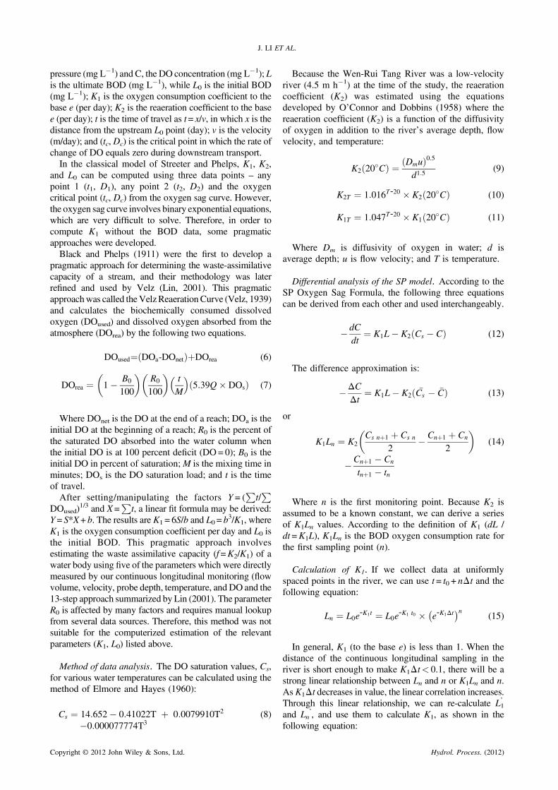
J LI ET AL
pressure (mg L1) and C the DO concentration (mg L1) Lis the ultimate BOD (mg L1) while L0 is the initial BOD(mg L1) K1 is the oxygen consumption coefficient to thebase e (per day) K2 is the reaeration coefficient to the basee (per day) t is the time of travel as t= xv in which x is thedistance from the upstream L0 point (day) v is the velocity(mday) and (tc Dc) is the critical point in which the rate ofchange of DO equals zero during downstream transportIn the classical model of Streeter and Phelps K1 K2
and L0 can be computed using three data points ndash anypoint 1 (t1 D1) any point 2 (t2 D2) and the oxygencritical point (tc Dc) from the oxygen sag curve Howeverthe oxygen sag curve involves binary exponential equationswhich are very difficult to solve Therefore in order tocompute K1 without the BOD data some pragmaticapproaches were developedBlack and Phelps (1911) were the first to develop a
pragmatic approach for determining the waste-assimilativecapacity of a stream and their methodology was laterrefined and used by Velz (Lin 2001) This pragmaticapproachwas called theVelzReaerationCurve (Velz 1939)and calculates the biochemically consumed dissolvedoxygen (DOused) and dissolved oxygen absorbed from theatmosphere (DOrea) by the following two equations
DOusedfrac14 DOa-DOneteth THORNthornDOrea (6)
DOrea frac14 1 B0
100
R0
100
t
M
539Q DOseth THORN (7)
Where DOnet is the DO at the end of a reach DOa is theinitial DO at the beginning of a reach R0 is the percent ofthe saturated DO absorbed into the water column whenthe initial DO is at 100 percent deficit (DO= 0) B0 is theinitial DO in percent of saturationM is the mixing time inminutes DOs is the DO saturation load and t is the timeof travelAfter settingmanipulating the factors Y = (
PtP
DOused)13 and X=
Pt a linear fit formula may be derived
Y= SX+ b The results are K1 = 6Sb and L0 = b3K1 where
K1 is the oxygen consumption coefficient per day and L0 isthe initial BOD This pragmatic approach involvesestimating the waste assimilative capacity (f=K2K1) of awater body using five of the parameters which were directlymeasured by our continuous longitudinal monitoring (flowvolume velocity probe depth temperature and DO and the13-step approach summarized by Lin (2001) The parameterR0 is affected by many factors and requires manual lookupfrom several data sources Therefore this method was notsuitable for the computerized estimation of the relevantparameters (K1 L0) listed above
Method of data analysis The DO saturation values Csfor various water temperatures can be calculated using themethod of Elmore and Hayes (1960)
Cs frac14 14652 041022T thorn 00079910T2
0000077774T3(8)
Copyright copy 2012 John Wiley amp Sons Ltd
Because the Wen-Rui Tang River was a low-velocityriver (45 m h1) at the time of the study the reaerationcoefficient (K2) was estimated using the equationsdeveloped by OrsquoConnor and Dobbins (1958) where thereaeration coefficient (K2) is a function of the diffusivityof oxygen in addition to the riverrsquos average depth flowvelocity and temperature
K2 20Ceth THORN frac14 Dmueth THORN05d15
(9)
K2T frac14 1016T-20 K2 20Ceth THORN (10)
K1T frac14 1047T-20 K1 20Ceth THORN (11)
Where Dm is diffusivity of oxygen in water d isaverage depth u is flow velocity and T is temperature
Differential analysis of the SP model According to theSP Oxygen Sag Formula the following three equationscan be derived from each other and used interchangeably
dC
dtfrac14 K1L K2 Cs Ceth THORN (12)
The difference approximation is
ΔCΔt
frac14 K1L K2 Cs Ceth THORN (13)
or
K1Ln frac14 K2Cs nthorn1 thorn Cs n
2 Cnthorn1 thorn Cn
2
Cnthorn1 Cn
tnthorn1 tn
(14)
Where n is the first monitoring point Because K2 isassumed to be a known constant we can derive a seriesof K1Ln values According to the definition of K1 (dL dt =K1L) K1Ln is the BOD oxygen consumption rate forthe first sampling point (n)
Calculation of K1 If we collect data at uniformlyspaced points in the river we can use t= t0 + nΔt and thefollowing equation
Ln frac14 L0e-K1t frac14 L0e
-K1 t0 e-K1Δt n
(15)
In general K1 (to the base e) is less than 1 When thedistance of the continuous longitudinal sampling in theriver is short enough to make K1Δtlt 01 there will be astrong linear relationship between Ln and n or K1Ln and nAs K1Δt decreases in value the linear correlation increasesThrough this linear relationship we can re-calculate Lrsquo1and Ln
rsquo and use them to calculate K1 as shown in thefollowing equation
Hydrol Process (2012)
MONITORING AND MODELING DISSOLVED OXYGEN DYNAMICS IN SURFACE WATERS
K1 frac14 1n-1eth THORNΔt LN
L01
L0n
frac14 1n-1eth THORNΔt LN
K1L01
K1L0n
(16)
Selection of DO data meeting the SP model assumptionsand for point source assessment The SP model is a one-dimensional steady-state model for DO-BOD relation-ships In theory it requires an instantaneous mixing of thesewage with the river water throughout the river crosssection In reality near the sewage outlet this isimpossible Therefore we must identify the DO datafrom the continuous monitoring data which are suitablefor use in the SP model Ideally these data should befrom the section where the sewage has already beenuniformly mixed with the water column and indicated bya good linear relationship between K1Ln and n At bothends of the longitudinal DO data set the DO data deviateappreciably from this linear relationship so these datawere discardedWe were also able to assess locations of point source
BOD inputs within the river reach In the longitudinal DOdata set the critical point is a key data parameter in whichthe rate of change for DO is zero and the key data (Cc tc)point was used to compute the initial BOD (L0) using thefollowing formula
L0 frac14 Cs-Cceth THORN K2
K1 eK1tc (17)
The initial BOD (L0) is composed of two parts one partof the discharge stems from the sewage outlet Loutletwhile the other part originates from BOD imported fromupstream sewage L0rsquo (Loutlet = L0 - L0rsquo)
Figure 2 Dissolved Oxygen (DO) variations in Hualongqiao River fromupstream to downstream DO is percent of saturation The light blue showsthe river width in the sampled segment similarly as shown in Figure 3 and 4
RESULTS
Table I provides an example of the continuous longitu-dinal data and its structure Among the total of 180 datapoints collected along the 2014 m river segment (~112 m
Table I Longitudinal continuous
Temp CondTime lat Long C S cm1
141734 1206705 279869 253 025141739 1206706 279870 253 025141744 1206707 279870 253 025141749 1206708 279871 252 025 143249 1206873 279933 257 025143254 1206875 279934 257 025143334 1206883 279939 254 026143339 1206884 279940 255 026
Copyright copy 2012 John Wiley amp Sons Ltd
between sampling points) there were 36 data pointswhich lacked GPS coordinates because the GPS receivercould not receive satellite signals when the boat navigatedunder bridges These missing GPS coordinates wereinterpolated between measured GPS points assuming auniform boat speed of 806 km h1
Trend of dissolved oxygen and identification of the hiddendrainage outlets
The average DO concentration was 218 of saturation(which is equivalent to 175 mg L1) and ranged from 94(076 mg L1) to 364 (29 mg L1) (Figure 2) Averagetotal ammonia nitrogen concentration was 725 mg L1ranging from 593 to 816 mg L1 (Figure 3) with manypeaks within the river segment Water temperaturedisplayed about a 1C variation along the river segmentwith an average temperature of 256C (Figure 4) The peaksof temperature ammonia and DO occurred at a distance of700 m where a tributary joins the Hualongqiao River(Figures 2ndash4)Changes in DO concentrations along the river segment
are shown in Figure 5 According to the SP OxygenSag Curve Figure 5 displays eight positive peaks in theDO curve The rate of change ie ΔDOΔL was verifiedto correspond to the maximum BOD concentrations asshown by the red solid line in Figure 5 which are relatedto the locations of eight sewage drainage outlets (pointsources) The minimum values in the DO curve (when
water quality monitoring data
Probe Depth Ammonium-N Turb DOm pH mg L1 NTU
01 671 73 236 12301 670 75 225 11301 670 77 214 10601 670 78 203 99
01 676 71 64 25001 676 69 63 25801 675 74 71 18901 675 74 70 204
Hydrol Process (2012)
Figure 3 Ammonium-N variations in Hualongqiao River from upstreamto downstream
Figure 4 Temperature variations in Hualongqiao River from upstream todownstream
Figure 5 DO variations and DO rate of variations in Hualongqiao Riverfrom upstream to downstream The symbols from A1 to A8 are thepositions of the sewage outlets based on the analysis of DO peaks andverified in the field The DO rates of variations are only shown between
the two sewage outlets
J LI ET AL
ΔDOΔL= 0) are identified as the critical points atwhich DO rate of change is equal to zero The SPOxygen Sag Curve will show a single maximum andminimum peak in the trend of DO if there is only onewastewater outlet in a river However eight such twinpeaks (maxima and minima) were observed in Figure 5which correspond to eight major sewage outlets in theriver segment The locations of the outlets designated A1through A8 in Figure 5 were verified by the fieldinvestigation This revelation shows that the continuous
Copyright copy 2012 John Wiley amp Sons Ltd
longitudinal sampling for DO can accurately identify thehidden sewage outlets under the water surface
Calculation of K1 the oxygen consumption coefficient
In general K1 to the base e is considered to be aconstant Therefore K1 was calculated using the DO datain the A4ndashA5 segment shown in Figure 5 This riversegment contains more monitoring points resulting in asmooth curve that indicates that there are no majorwastewater sources in this segment The DO data for theA4ndashA5 segment and related parameters used to calculateK1 are listed in Table IIIn the case study Δt = 01147 and K1lt 08 so
K1Δtlt 01 Since the value of K1Δt was much smallerthan the threshold of 095 (as defined in section 244) astrong linear relationship between K1Ln and n wasexpected Figure 6 shows the linear relationship betweenK1Ln and n using the DO data from the A4ndashA5 riversegment Based on Equation (17) oxygen consumptioncoefficients (K1) of 0552 d1 (25C) and 0428 d1
(20C) were obtainedWhen the Velz Reaeration Curve was used to
independently calculate K1 results were b = 0193S = 0017 and K1 = 6sb = 0528 d1 The results of thetwo K1 estimation approaches using our derived approachand the Velz Reaeration Curve were similar (0552 vs0528 d1 25C) supporting the validity of using our newapproach in calculating K1
Calculation of L0 and assessment of point source pollution
The calculated BOD discharge loads from wastewateroutlets A1 to A8 are listed in Table III Outlets A5 andA7 released the largest amount of BOD at 226 and 234 kgd1 respectively followed by the outlets A1 and A4 at104 and 121 kg d1 respectively while outlets A2 A3A6 and A8 released BOD loads of less than 100 kg d1
(Table III) The sum of BOD loads from the eight outletsindicates the total amount of BOD discharged into theriver segment examined in this study was 916 kg d1
Computation of self-purification capacity
The BOD assimilative capacity (K2K1) ie self-purification capacity was calculated based on designatedminimum DO values which correspond to the criticalpoints of the oxygen sag curve We assumed that thesewage outlets in the river were upstream and thatthe amount of the initial DO was equal to the amountof DO at saturation or D0 = 0 Following the analysis ofinferences in Section 244 286 days (tc) wererequired for DO to change from the highest value tothe lowest valueThe minimum dissolved oxygen (Dc) of the river was set
to four water quality standard values ranging from 2ndash6 mgL1 which correspond to four water quality classificationgrades in China The results of the computation for BODload capacity ranged from 129 kg d1 to maintain the 6 mgL1 DO minimum standard to 382 kg d1 to maintain the2 mg L1 DO minimum standard (Table IV)
Hydrol Process (2012)
Table II Calculation of K1 using the DO data in A4ndashA5 segment
Length Temp C Cs Mean Cs Mean C ΔtNo meter C mg L1 mg L1 mg L1 mg L1 days ΔC K2 K1L n
74 00 263 290 797 0 020775 128 258 265 806 801 278 0118 025 0205 31976 127 256 232 809 807 249 0118 033 0204 39477 126 255 208 810 809 22 0117 024 0204 32678 126 255 195 810 810 202 0117 013 0204 236 179 125 255 187 810 810 191 0116 008 0204 195 280 124 255 180 810 810 184 0115 007 0204 189 381 124 255 175 811 810 178 0115 005 0204 174 482 124 254 171 811 811 173 0115 004 0204 165 583 123 254 166 811 811 169 0113 005 0204 175 684 123 254 163 811 811 165 0114 003 0204 158 785 122 254 161 811 811 162 0113 002 0204 150 886 122 255 162 811 811 162 0113 001 0204 124 987 123 255 164 810 810 163 0114 002 0204 115 1088 119 255 166 810 810 165 0110 002 0204 114 1189 123 255 167 810 810 167 0114 001 0204 123 1290 125 255 170 810 810 169 0116 003 0204 105 1391 126 255 173 810 810 172 0117 003 0204 105 1492 122 255 177 810 810 175 0113 004 0204 094 1593 121 255 183 810 810 18 0112 006 0204 075 1694 122 255 187 810 810 185 0113 004 0204 092
Notes Velocity = 000125ms Depth = 185m
Figure 6 The analysis of the linear relationship between K1Ln and n
Table III Assessment of point source pollution
L0 L00 Loutfall Flow Q LoutfallStation mg L1 mg L1 mg L1 m3 d1 kg d1
A1 30 00 30 35 191 104A2 33 20 13 35 191 46A3 25 082 17 35 191 59A4 49 14 34 35 191 120A5 78 14 64 35 191 226A6 28 08 20 35 191 69A7 79 12 66 35 191 234A8 35 19 17 35 191 58
Notes L0 is the initial BOD Lrsquo0 is the BOD from upstream Loutfall is thedischarge of the sewage outfall
Table IV Computation of self-purification capacity
DO standards Self-purification capacityWater quality types mgL mgL kgday
II 6 37 129III 5 55 192IV 3 90 318V 2 11 381
Notes Flow= 0407 m3 s1 Average temperature = 2552 C K2 = 0204d1 K1 = 0552 d1
Figure 7 Observed DO data and model prediction curve in HualongqiaoRiver
MONITORING AND MODELING DISSOLVED OXYGEN DYNAMICS IN SURFACE WATERS
Figure 7 shows that the observed DO (black line) washighly correlated (r= 068) with the model-generated DO(red line) concentrations along the river segment Thisanalysis indicated that the model reasonably predicted theDO values for the river segment in this study Since theSP model requires an unrealistic instantaneous mixing of
Copyright copy 2012 John Wiley amp Sons Ltd
the wastewater with the river water it is not surprisingthat the two large peaks for predicted DO do not matchwell with the observed DO
Hydrol Process (2012)
J LI ET AL
DISCUSSION
The calculated oxygen consumption coefficient (K1)varies with temperature as indicated by the value of0552 d1 at 256C (ambient) and 0428 d1 normalizedfor 20C The greater the K1 value the faster oxygen isbeing consumed Thus the relatively high K1 value in theHualongqiao River indicates that oxygen consumption israpid and that inputs of oxygen demanding substances arevery severe in this river segment This is consistent withthe water quality classification of inferior Type V (lt2 mgL1 O2) that is common throughout Wenzhou Citywaterways (Wenzhou State of the Environment 2008)The calculated BOD discharged into the river segment916 kg d1 was considerably higher than theBOD receivingload capacity for type V water quality of 381 kg d1 basedon the 2 mg L1 DO minimum Thus BOD discharge intothe river segment would need to be reduced by 535 kg d1 tomeet the minimumwater quality standard DO concentrationof 2 mg L1 This specific reduction target provides a usefulreference point for the municipal government to properlydevise water management decisionsThis theoretical analysis has practical implications for
water quality assessment By showing that the K1 andBOD assimilative capacity may be computed using onlyDO data collected in a rigorous longitudinal fashion thismethod obtains real-time water quality information usingfar less resources than traditional laboratory methodsAlthough the Velz Reaeration Curve (Velz 1939 Lin2001) also calculates an oxygen consumption coefficient(K1) using only DO data (K1 was 0528 d1 using theVelz Reaeration Curve) it is far more cumbersome ifcontinuous longitudinal DO data are not availableThe new monitoring and calculation approach analyzed
and demonstrated in this study is direct simple and suitablefor automated computer processing for water qualityassessment The ability to rapidly collect densely packedDO concentration measurements with high precision usingthe continuous longitudinal monitoring technology makesthis new approach possible in real times The oxygenconsumption coefficient (K1) is a critical parameter drivingoxygen dynamics in many water quality models such as theEPD-RIV1 and QUAL2K developed by the US Environ-mental ProtectionAgency However with the application ofthese water quality models parameter calibration has been akey problem that is difficult to resolve with confidence Thedata collection and analysis methods proposed in this studycan be used to spatially determine the critical oxygenconsumption coefficient (K1) for a given watershed Thisapproach is especially useful in highly polluted riverswhich are common in many rapidly developing countriesThe essence of this approach is the use of dense DO
sampling to obtain the rate of change for DO concentrationsallowing the use ofΔCΔt instead of dCdt in the differentialequations used to describe the BOD-DO relationships Thisgreatly reduces the difficulty of solving the differentialequations Dense sampling requires data collectionmethods that are convenient fast reliable and low costThe continuous longitudinal water quality monitoring using
Copyright copy 2012 John Wiley amp Sons Ltd
sondes with multiple sensors meets these requirementsHowever to facilitate subsequent data analysis and optimizemodel results some additional requirements for samplingfrequency and uniform sampling distance by continuouslongitudinal monitoring must be met
Data quality and its influence
A sensitivity analysis examining experimental variabilityin water quality data acquired by the YSI sonde in this studyindicates low (lt2) variability in predicted parametersbased on the expected sonde variability The YSI 6150Optical DO sensor uses a fast interception system formeasuring DO This type of fast interception system uses aClark sensor to measure the return of electrons diffusedthrough a Teflon membrane The accuracy of DO measure-ments is influenced by temperature and the flow of the watersystem around the sonde Temperature was automaticallycorrected using the measured water temperatures Basedon the YSI userrsquos manual DO readings will be decreased by2ndash3 at the speed of our boat compared to DO readingsin still water Considering this difference we recalculatethe K1 as 0554 ~ 0556 d
1 (25C) compared to K1 = 0552d1 (25C) for non-velocity corrected values Thesedifferences result in K1 value differences 04ndash07 lowerand L0 values 07ndash1 higher Since all DO measurementswere taken at a constant boat travel velocity all of ourmeasurements are internally consistent
Sampling frequency requirements
The continuous longitudinal monitoring of rivers isactually a kind of digitization of the continuous DO dataTherefore in accordance with the requirements of theSamplingTheorem (Shannon 1949) the sampling frequencymust be greater than twice the highest frequency of the analogsignals Under this condition the sampling results may befully representative of the original analog signal For bestresults with respect to real-world sampling the samplingfrequency should be set as three to five times the highestsignal frequency The SP model requires an instantaneousmixing of the wastewater with the river water to produce avalid sampling point but these mixing conditions near thesewage outlets are not possible to fully achieve Consideringthese factors we set the sampling frequency at eight timeshigher than the signal frequency In the river segmentexamined the minimum distance between the identifiedsewage outlets was 85 m therefore the distance betweenmonitoring points was set to approximately 11 m (858 m)
Limitation and applicability
The application of continuous longitudinal water qualitysampling data provides a theoretical basis for obtaining theoxygen consumption coefficient which is otherwise difficultto acquire however there are some limitations One of theconditions required to maintain the linear relationshipbetween K1L and n is a uniform Δt If we assume that thewater flow rate is constant this is accomplished byuniformly spaced sampling times (5 s interval in this study)The water quality sonde is fixed on the boat which must
Hydrol Process (2012)
MONITORING AND MODELING DISSOLVED OXYGEN DYNAMICS IN SURFACE WATERS
move at a uniform speed to meet the uniform samplingdistance requirement The continuous longitudinal monitor-ing method presented here is also one dimensional so themonitoring boat must move along the center line of the riverto achieve optimum data collection In addition due to thespecific conditions of the river segment examined twocomplicated terms in the equations were considerednegligible Future research may explore the non-linearrelationships between the K1L and n as well as expandingthe analysis to two- or three-dimensional calculations of theessential water quality parameters for broader application tosustainable water resource management
CONCLUSION
This study used a branch of the Wen-Rui Tang River asa case study to demonstrate the efficacy of using alongitudinal continuous water quality monitoring method-ology to model BOD-DO dynamics in a hypoxic urbanriver The results indicated that continuous longitudinalmonitoring of temperature and DO is a powerful approachfor quantifying several BOD-DO parameters This methodallows direct computation of the oxygen consumptioncoefficient (K1) BOD assimilative capacity BOD pointsource locations and total BOD loads discharged into theriver segment of interest With these values we are able tobetter evaluate changes in water quality and chart thecontinuous temporal and spatial distributions of BOD-DOdynamics in complex urban waterways This approach canbe applied to any other complex urban waterways with slowflow movement for water quality assessment
ACKNOWLEDGEMENTS
This research was fully funded by Science and TechnologyDepartment of Zhejiang Province China through ProjectNo 2008C03009 Wenzhou River Assessment Officethrough Project No 20082780125 Authors wish to thankDr Michael Grieneisen for improving the English in thepaper Authors would also like to thank the editor andthe anonymous reviewers for constructive comments toimprove the paper
REFERENCES
Adrian DD Yu FX Barbe D 1994 Water quality modeling for asinusoidally varying waste discharge concentrations Water Research28 1167ndash1174
AsianInfo Services 2004 Wenzhou treats river with biological remediationtechnology httpwwwallbusinesscomenvironment-natural-resourcespollution7687802ndash1
Beck MB Young PC 1976 Systematic identification of DO-BOD modelstructure Journal of the Environmental Engineering Division ASCE102 902ndash927
Black WM Phelps EB 1911 Location of sewer outlets and discharge ofsewage in New York Harbor New York City Board of Estimate andApportionment March 23 1911
Brown LC Barnwell TO 1987 The enhanced stream water qualitymodels QUAL2E and QUAL2E-UNCAS documentation and user
Copyright copy 2012 John Wiley amp Sons Ltd
manual Environmental Research Laboratory US EPA WashingtonDC
Camp TR 1963 First expanded BOD-DO model In Basic River WaterQuality Models (IHP-V Project 81) Jolankai DG (ed) UNESCOPublications Paris 27ndash29
Chapra SC Pelletier GJ 2003 QUAL2K A Modeling Framework forSimulating River and Stream Water Quality Documentation and UsersManual [J] Civil and Environmental Engineering Dept TuftsUniversity Medford
Elmore HL Hayes TW 1960 Solubility of atmospheric oxygen inwater Journal of the Sanitation Engineering Division ASCE 8641ndash53
Fair GM 1939 The dissolved oxygen sagmdashan analysis Sewage WorksJournal 11 445ndash461
Gotovtsev AV 2010 Modification of the StreeterndashPhelps system withthe aim to account for the feedback between dissolved oxygenconcentration and organic matter oxidation rate Water Resources 37245ndash251
Gundelach JM Castillo JE 1976 Natural stream purification underanaerobic conditions Journal Water Pollution Control Federation 481753ndash1758
Jolankai G 1997 Basic river water quality models Technical Documentsin Hydrology no 13 IHP-V UNESCO Paris 50
Li WH 1962 Unsteady dissolved-oxygen sag in a stream Journal of theEnvironmental Engineering Division ASCE 88 75ndash85
Li WH 1972 Effects of dispersion on DO-SAG in uniform flow Journalof the Environmental Engineering Division ASCE 98 169ndash182
Lin SD 2001 Water and wastewater calculation manual McGrow-HillCompanies USA 854
Martin JL Wool TA 2002 A dynamic one-dimensional modelofhydrodynamics and water quality (EPD-RIV1)version 10ModelDocumentation and User Manual Georgia Environmental ProtectionDivision Atlanta GA
OrsquoConnor DJ Dobbins WE 1958 The mechanism of reaeration in naturalstreams Journal of the Environmental Engineering Division ASCE123 641ndash684
Shannon CE 1949 Communication in the presence of noise ProceedingsInstitute of Radio Engineers 37 10ndash21
State Environmental Protection Administration of China 2005 ChinaUrban Environmental Management 200562 P12
Streeter HW Phelps EB 1925 A Study of the pollution and naturalpurification of the Ohio river III Factors concerned in the phenomenaof oxidation and reaeration Public Health Bulletin no 146 Reprintedby US Department of Health Education and Welfare Public HealthService 1958 ISBN B001BP4GZI httpdspaceudeledu8080dspacebitstreamhandle197161590C26EE148pdfsequence=2
Tase N Arai H Suzumura T 1993 Use of 15N isotope as a natural tracerfor evaluating self-purification in the Tamagawa Jousui ChannelInternational Association of Hydrological Sciences Publications 215225ndash231
Theriault EJ 1927 The dissolved oxygen demand of polluted watersPublic Health Bulletin no 173 US Public Health Service WashingtonDC 189
Thomann RV Muumlller JA 1987 Principles of Surface Water QualityModelling and Control Harper amp Row New York
Thomas HA 1948 Pollution load capacity of streams Water amp SewageWorks 95 409ndash413
Velz CJ 1939 Deoxygenation and reoxygenation Transactions of theAmerican Society of Civil Engineers 104 560ndash572
Voss S 2011 Industrial pollution kills hundreds along the Huai RiverBasin in China httpwwwstephenvosscomstoriesChinaWaterPollu-tionstoryhtml Available October 15 2011
Wenzhou State of the Environment 2008 The State of Environment inWenzhou in 2008 httpwwwouhaigovcnart200965art_2175_21881html
Wool TA Ambrose RB Martin JL Comer EA 2001 US EnvironmentalProtection AgencyndashRegion Atlanta GA Environmental ResearchLaboratory Athens GA USACE ndash Waterways Experiment StationVicksburg MS Tetra Tech Inc Atlanta GA
Yu FX Adrian DD Singh P 1991 Modeling river quality by thesuperposition method Journal of Environmental Systems 20 1ndash16
Zhang J Mauzerall DL Zhu T Liang S Ezzati M Remais JV 2010Environmental health in China Progress toward clean air and safewater Lancet 375 1110ndash1119
Hydrol Process (2012)

MONITORING AND MODELING DISSOLVED OXYGEN DYNAMICS IN SURFACE WATERS
K1 frac14 1n-1eth THORNΔt LN
L01
L0n
frac14 1n-1eth THORNΔt LN
K1L01
K1L0n
(16)
Selection of DO data meeting the SP model assumptionsand for point source assessment The SP model is a one-dimensional steady-state model for DO-BOD relation-ships In theory it requires an instantaneous mixing of thesewage with the river water throughout the river crosssection In reality near the sewage outlet this isimpossible Therefore we must identify the DO datafrom the continuous monitoring data which are suitablefor use in the SP model Ideally these data should befrom the section where the sewage has already beenuniformly mixed with the water column and indicated bya good linear relationship between K1Ln and n At bothends of the longitudinal DO data set the DO data deviateappreciably from this linear relationship so these datawere discardedWe were also able to assess locations of point source
BOD inputs within the river reach In the longitudinal DOdata set the critical point is a key data parameter in whichthe rate of change for DO is zero and the key data (Cc tc)point was used to compute the initial BOD (L0) using thefollowing formula
L0 frac14 Cs-Cceth THORN K2
K1 eK1tc (17)
The initial BOD (L0) is composed of two parts one partof the discharge stems from the sewage outlet Loutletwhile the other part originates from BOD imported fromupstream sewage L0rsquo (Loutlet = L0 - L0rsquo)
Figure 2 Dissolved Oxygen (DO) variations in Hualongqiao River fromupstream to downstream DO is percent of saturation The light blue showsthe river width in the sampled segment similarly as shown in Figure 3 and 4
RESULTS
Table I provides an example of the continuous longitu-dinal data and its structure Among the total of 180 datapoints collected along the 2014 m river segment (~112 m
Table I Longitudinal continuous
Temp CondTime lat Long C S cm1
141734 1206705 279869 253 025141739 1206706 279870 253 025141744 1206707 279870 253 025141749 1206708 279871 252 025 143249 1206873 279933 257 025143254 1206875 279934 257 025143334 1206883 279939 254 026143339 1206884 279940 255 026
Copyright copy 2012 John Wiley amp Sons Ltd
between sampling points) there were 36 data pointswhich lacked GPS coordinates because the GPS receivercould not receive satellite signals when the boat navigatedunder bridges These missing GPS coordinates wereinterpolated between measured GPS points assuming auniform boat speed of 806 km h1
Trend of dissolved oxygen and identification of the hiddendrainage outlets
The average DO concentration was 218 of saturation(which is equivalent to 175 mg L1) and ranged from 94(076 mg L1) to 364 (29 mg L1) (Figure 2) Averagetotal ammonia nitrogen concentration was 725 mg L1ranging from 593 to 816 mg L1 (Figure 3) with manypeaks within the river segment Water temperaturedisplayed about a 1C variation along the river segmentwith an average temperature of 256C (Figure 4) The peaksof temperature ammonia and DO occurred at a distance of700 m where a tributary joins the Hualongqiao River(Figures 2ndash4)Changes in DO concentrations along the river segment
are shown in Figure 5 According to the SP OxygenSag Curve Figure 5 displays eight positive peaks in theDO curve The rate of change ie ΔDOΔL was verifiedto correspond to the maximum BOD concentrations asshown by the red solid line in Figure 5 which are relatedto the locations of eight sewage drainage outlets (pointsources) The minimum values in the DO curve (when
water quality monitoring data
Probe Depth Ammonium-N Turb DOm pH mg L1 NTU
01 671 73 236 12301 670 75 225 11301 670 77 214 10601 670 78 203 99
01 676 71 64 25001 676 69 63 25801 675 74 71 18901 675 74 70 204
Hydrol Process (2012)
Figure 3 Ammonium-N variations in Hualongqiao River from upstreamto downstream
Figure 4 Temperature variations in Hualongqiao River from upstream todownstream
Figure 5 DO variations and DO rate of variations in Hualongqiao Riverfrom upstream to downstream The symbols from A1 to A8 are thepositions of the sewage outlets based on the analysis of DO peaks andverified in the field The DO rates of variations are only shown between
the two sewage outlets
J LI ET AL
ΔDOΔL= 0) are identified as the critical points atwhich DO rate of change is equal to zero The SPOxygen Sag Curve will show a single maximum andminimum peak in the trend of DO if there is only onewastewater outlet in a river However eight such twinpeaks (maxima and minima) were observed in Figure 5which correspond to eight major sewage outlets in theriver segment The locations of the outlets designated A1through A8 in Figure 5 were verified by the fieldinvestigation This revelation shows that the continuous
Copyright copy 2012 John Wiley amp Sons Ltd
longitudinal sampling for DO can accurately identify thehidden sewage outlets under the water surface
Calculation of K1 the oxygen consumption coefficient
In general K1 to the base e is considered to be aconstant Therefore K1 was calculated using the DO datain the A4ndashA5 segment shown in Figure 5 This riversegment contains more monitoring points resulting in asmooth curve that indicates that there are no majorwastewater sources in this segment The DO data for theA4ndashA5 segment and related parameters used to calculateK1 are listed in Table IIIn the case study Δt = 01147 and K1lt 08 so
K1Δtlt 01 Since the value of K1Δt was much smallerthan the threshold of 095 (as defined in section 244) astrong linear relationship between K1Ln and n wasexpected Figure 6 shows the linear relationship betweenK1Ln and n using the DO data from the A4ndashA5 riversegment Based on Equation (17) oxygen consumptioncoefficients (K1) of 0552 d1 (25C) and 0428 d1
(20C) were obtainedWhen the Velz Reaeration Curve was used to
independently calculate K1 results were b = 0193S = 0017 and K1 = 6sb = 0528 d1 The results of thetwo K1 estimation approaches using our derived approachand the Velz Reaeration Curve were similar (0552 vs0528 d1 25C) supporting the validity of using our newapproach in calculating K1
Calculation of L0 and assessment of point source pollution
The calculated BOD discharge loads from wastewateroutlets A1 to A8 are listed in Table III Outlets A5 andA7 released the largest amount of BOD at 226 and 234 kgd1 respectively followed by the outlets A1 and A4 at104 and 121 kg d1 respectively while outlets A2 A3A6 and A8 released BOD loads of less than 100 kg d1
(Table III) The sum of BOD loads from the eight outletsindicates the total amount of BOD discharged into theriver segment examined in this study was 916 kg d1
Computation of self-purification capacity
The BOD assimilative capacity (K2K1) ie self-purification capacity was calculated based on designatedminimum DO values which correspond to the criticalpoints of the oxygen sag curve We assumed that thesewage outlets in the river were upstream and thatthe amount of the initial DO was equal to the amountof DO at saturation or D0 = 0 Following the analysis ofinferences in Section 244 286 days (tc) wererequired for DO to change from the highest value tothe lowest valueThe minimum dissolved oxygen (Dc) of the river was set
to four water quality standard values ranging from 2ndash6 mgL1 which correspond to four water quality classificationgrades in China The results of the computation for BODload capacity ranged from 129 kg d1 to maintain the 6 mgL1 DO minimum standard to 382 kg d1 to maintain the2 mg L1 DO minimum standard (Table IV)
Hydrol Process (2012)
Table II Calculation of K1 using the DO data in A4ndashA5 segment
Length Temp C Cs Mean Cs Mean C ΔtNo meter C mg L1 mg L1 mg L1 mg L1 days ΔC K2 K1L n
74 00 263 290 797 0 020775 128 258 265 806 801 278 0118 025 0205 31976 127 256 232 809 807 249 0118 033 0204 39477 126 255 208 810 809 22 0117 024 0204 32678 126 255 195 810 810 202 0117 013 0204 236 179 125 255 187 810 810 191 0116 008 0204 195 280 124 255 180 810 810 184 0115 007 0204 189 381 124 255 175 811 810 178 0115 005 0204 174 482 124 254 171 811 811 173 0115 004 0204 165 583 123 254 166 811 811 169 0113 005 0204 175 684 123 254 163 811 811 165 0114 003 0204 158 785 122 254 161 811 811 162 0113 002 0204 150 886 122 255 162 811 811 162 0113 001 0204 124 987 123 255 164 810 810 163 0114 002 0204 115 1088 119 255 166 810 810 165 0110 002 0204 114 1189 123 255 167 810 810 167 0114 001 0204 123 1290 125 255 170 810 810 169 0116 003 0204 105 1391 126 255 173 810 810 172 0117 003 0204 105 1492 122 255 177 810 810 175 0113 004 0204 094 1593 121 255 183 810 810 18 0112 006 0204 075 1694 122 255 187 810 810 185 0113 004 0204 092
Notes Velocity = 000125ms Depth = 185m
Figure 6 The analysis of the linear relationship between K1Ln and n
Table III Assessment of point source pollution
L0 L00 Loutfall Flow Q LoutfallStation mg L1 mg L1 mg L1 m3 d1 kg d1
A1 30 00 30 35 191 104A2 33 20 13 35 191 46A3 25 082 17 35 191 59A4 49 14 34 35 191 120A5 78 14 64 35 191 226A6 28 08 20 35 191 69A7 79 12 66 35 191 234A8 35 19 17 35 191 58
Notes L0 is the initial BOD Lrsquo0 is the BOD from upstream Loutfall is thedischarge of the sewage outfall
Table IV Computation of self-purification capacity
DO standards Self-purification capacityWater quality types mgL mgL kgday
II 6 37 129III 5 55 192IV 3 90 318V 2 11 381
Notes Flow= 0407 m3 s1 Average temperature = 2552 C K2 = 0204d1 K1 = 0552 d1
Figure 7 Observed DO data and model prediction curve in HualongqiaoRiver
MONITORING AND MODELING DISSOLVED OXYGEN DYNAMICS IN SURFACE WATERS
Figure 7 shows that the observed DO (black line) washighly correlated (r= 068) with the model-generated DO(red line) concentrations along the river segment Thisanalysis indicated that the model reasonably predicted theDO values for the river segment in this study Since theSP model requires an unrealistic instantaneous mixing of
Copyright copy 2012 John Wiley amp Sons Ltd
the wastewater with the river water it is not surprisingthat the two large peaks for predicted DO do not matchwell with the observed DO
Hydrol Process (2012)
J LI ET AL
DISCUSSION
The calculated oxygen consumption coefficient (K1)varies with temperature as indicated by the value of0552 d1 at 256C (ambient) and 0428 d1 normalizedfor 20C The greater the K1 value the faster oxygen isbeing consumed Thus the relatively high K1 value in theHualongqiao River indicates that oxygen consumption israpid and that inputs of oxygen demanding substances arevery severe in this river segment This is consistent withthe water quality classification of inferior Type V (lt2 mgL1 O2) that is common throughout Wenzhou Citywaterways (Wenzhou State of the Environment 2008)The calculated BOD discharged into the river segment916 kg d1 was considerably higher than theBOD receivingload capacity for type V water quality of 381 kg d1 basedon the 2 mg L1 DO minimum Thus BOD discharge intothe river segment would need to be reduced by 535 kg d1 tomeet the minimumwater quality standard DO concentrationof 2 mg L1 This specific reduction target provides a usefulreference point for the municipal government to properlydevise water management decisionsThis theoretical analysis has practical implications for
water quality assessment By showing that the K1 andBOD assimilative capacity may be computed using onlyDO data collected in a rigorous longitudinal fashion thismethod obtains real-time water quality information usingfar less resources than traditional laboratory methodsAlthough the Velz Reaeration Curve (Velz 1939 Lin2001) also calculates an oxygen consumption coefficient(K1) using only DO data (K1 was 0528 d1 using theVelz Reaeration Curve) it is far more cumbersome ifcontinuous longitudinal DO data are not availableThe new monitoring and calculation approach analyzed
and demonstrated in this study is direct simple and suitablefor automated computer processing for water qualityassessment The ability to rapidly collect densely packedDO concentration measurements with high precision usingthe continuous longitudinal monitoring technology makesthis new approach possible in real times The oxygenconsumption coefficient (K1) is a critical parameter drivingoxygen dynamics in many water quality models such as theEPD-RIV1 and QUAL2K developed by the US Environ-mental ProtectionAgency However with the application ofthese water quality models parameter calibration has been akey problem that is difficult to resolve with confidence Thedata collection and analysis methods proposed in this studycan be used to spatially determine the critical oxygenconsumption coefficient (K1) for a given watershed Thisapproach is especially useful in highly polluted riverswhich are common in many rapidly developing countriesThe essence of this approach is the use of dense DO
sampling to obtain the rate of change for DO concentrationsallowing the use ofΔCΔt instead of dCdt in the differentialequations used to describe the BOD-DO relationships Thisgreatly reduces the difficulty of solving the differentialequations Dense sampling requires data collectionmethods that are convenient fast reliable and low costThe continuous longitudinal water quality monitoring using
Copyright copy 2012 John Wiley amp Sons Ltd
sondes with multiple sensors meets these requirementsHowever to facilitate subsequent data analysis and optimizemodel results some additional requirements for samplingfrequency and uniform sampling distance by continuouslongitudinal monitoring must be met
Data quality and its influence
A sensitivity analysis examining experimental variabilityin water quality data acquired by the YSI sonde in this studyindicates low (lt2) variability in predicted parametersbased on the expected sonde variability The YSI 6150Optical DO sensor uses a fast interception system formeasuring DO This type of fast interception system uses aClark sensor to measure the return of electrons diffusedthrough a Teflon membrane The accuracy of DO measure-ments is influenced by temperature and the flow of the watersystem around the sonde Temperature was automaticallycorrected using the measured water temperatures Basedon the YSI userrsquos manual DO readings will be decreased by2ndash3 at the speed of our boat compared to DO readingsin still water Considering this difference we recalculatethe K1 as 0554 ~ 0556 d
1 (25C) compared to K1 = 0552d1 (25C) for non-velocity corrected values Thesedifferences result in K1 value differences 04ndash07 lowerand L0 values 07ndash1 higher Since all DO measurementswere taken at a constant boat travel velocity all of ourmeasurements are internally consistent
Sampling frequency requirements
The continuous longitudinal monitoring of rivers isactually a kind of digitization of the continuous DO dataTherefore in accordance with the requirements of theSamplingTheorem (Shannon 1949) the sampling frequencymust be greater than twice the highest frequency of the analogsignals Under this condition the sampling results may befully representative of the original analog signal For bestresults with respect to real-world sampling the samplingfrequency should be set as three to five times the highestsignal frequency The SP model requires an instantaneousmixing of the wastewater with the river water to produce avalid sampling point but these mixing conditions near thesewage outlets are not possible to fully achieve Consideringthese factors we set the sampling frequency at eight timeshigher than the signal frequency In the river segmentexamined the minimum distance between the identifiedsewage outlets was 85 m therefore the distance betweenmonitoring points was set to approximately 11 m (858 m)
Limitation and applicability
The application of continuous longitudinal water qualitysampling data provides a theoretical basis for obtaining theoxygen consumption coefficient which is otherwise difficultto acquire however there are some limitations One of theconditions required to maintain the linear relationshipbetween K1L and n is a uniform Δt If we assume that thewater flow rate is constant this is accomplished byuniformly spaced sampling times (5 s interval in this study)The water quality sonde is fixed on the boat which must
Hydrol Process (2012)
MONITORING AND MODELING DISSOLVED OXYGEN DYNAMICS IN SURFACE WATERS
move at a uniform speed to meet the uniform samplingdistance requirement The continuous longitudinal monitor-ing method presented here is also one dimensional so themonitoring boat must move along the center line of the riverto achieve optimum data collection In addition due to thespecific conditions of the river segment examined twocomplicated terms in the equations were considerednegligible Future research may explore the non-linearrelationships between the K1L and n as well as expandingthe analysis to two- or three-dimensional calculations of theessential water quality parameters for broader application tosustainable water resource management
CONCLUSION
This study used a branch of the Wen-Rui Tang River asa case study to demonstrate the efficacy of using alongitudinal continuous water quality monitoring method-ology to model BOD-DO dynamics in a hypoxic urbanriver The results indicated that continuous longitudinalmonitoring of temperature and DO is a powerful approachfor quantifying several BOD-DO parameters This methodallows direct computation of the oxygen consumptioncoefficient (K1) BOD assimilative capacity BOD pointsource locations and total BOD loads discharged into theriver segment of interest With these values we are able tobetter evaluate changes in water quality and chart thecontinuous temporal and spatial distributions of BOD-DOdynamics in complex urban waterways This approach canbe applied to any other complex urban waterways with slowflow movement for water quality assessment
ACKNOWLEDGEMENTS
This research was fully funded by Science and TechnologyDepartment of Zhejiang Province China through ProjectNo 2008C03009 Wenzhou River Assessment Officethrough Project No 20082780125 Authors wish to thankDr Michael Grieneisen for improving the English in thepaper Authors would also like to thank the editor andthe anonymous reviewers for constructive comments toimprove the paper
REFERENCES
Adrian DD Yu FX Barbe D 1994 Water quality modeling for asinusoidally varying waste discharge concentrations Water Research28 1167ndash1174
AsianInfo Services 2004 Wenzhou treats river with biological remediationtechnology httpwwwallbusinesscomenvironment-natural-resourcespollution7687802ndash1
Beck MB Young PC 1976 Systematic identification of DO-BOD modelstructure Journal of the Environmental Engineering Division ASCE102 902ndash927
Black WM Phelps EB 1911 Location of sewer outlets and discharge ofsewage in New York Harbor New York City Board of Estimate andApportionment March 23 1911
Brown LC Barnwell TO 1987 The enhanced stream water qualitymodels QUAL2E and QUAL2E-UNCAS documentation and user
Copyright copy 2012 John Wiley amp Sons Ltd
manual Environmental Research Laboratory US EPA WashingtonDC
Camp TR 1963 First expanded BOD-DO model In Basic River WaterQuality Models (IHP-V Project 81) Jolankai DG (ed) UNESCOPublications Paris 27ndash29
Chapra SC Pelletier GJ 2003 QUAL2K A Modeling Framework forSimulating River and Stream Water Quality Documentation and UsersManual [J] Civil and Environmental Engineering Dept TuftsUniversity Medford
Elmore HL Hayes TW 1960 Solubility of atmospheric oxygen inwater Journal of the Sanitation Engineering Division ASCE 8641ndash53
Fair GM 1939 The dissolved oxygen sagmdashan analysis Sewage WorksJournal 11 445ndash461
Gotovtsev AV 2010 Modification of the StreeterndashPhelps system withthe aim to account for the feedback between dissolved oxygenconcentration and organic matter oxidation rate Water Resources 37245ndash251
Gundelach JM Castillo JE 1976 Natural stream purification underanaerobic conditions Journal Water Pollution Control Federation 481753ndash1758
Jolankai G 1997 Basic river water quality models Technical Documentsin Hydrology no 13 IHP-V UNESCO Paris 50
Li WH 1962 Unsteady dissolved-oxygen sag in a stream Journal of theEnvironmental Engineering Division ASCE 88 75ndash85
Li WH 1972 Effects of dispersion on DO-SAG in uniform flow Journalof the Environmental Engineering Division ASCE 98 169ndash182
Lin SD 2001 Water and wastewater calculation manual McGrow-HillCompanies USA 854
Martin JL Wool TA 2002 A dynamic one-dimensional modelofhydrodynamics and water quality (EPD-RIV1)version 10ModelDocumentation and User Manual Georgia Environmental ProtectionDivision Atlanta GA
OrsquoConnor DJ Dobbins WE 1958 The mechanism of reaeration in naturalstreams Journal of the Environmental Engineering Division ASCE123 641ndash684
Shannon CE 1949 Communication in the presence of noise ProceedingsInstitute of Radio Engineers 37 10ndash21
State Environmental Protection Administration of China 2005 ChinaUrban Environmental Management 200562 P12
Streeter HW Phelps EB 1925 A Study of the pollution and naturalpurification of the Ohio river III Factors concerned in the phenomenaof oxidation and reaeration Public Health Bulletin no 146 Reprintedby US Department of Health Education and Welfare Public HealthService 1958 ISBN B001BP4GZI httpdspaceudeledu8080dspacebitstreamhandle197161590C26EE148pdfsequence=2
Tase N Arai H Suzumura T 1993 Use of 15N isotope as a natural tracerfor evaluating self-purification in the Tamagawa Jousui ChannelInternational Association of Hydrological Sciences Publications 215225ndash231
Theriault EJ 1927 The dissolved oxygen demand of polluted watersPublic Health Bulletin no 173 US Public Health Service WashingtonDC 189
Thomann RV Muumlller JA 1987 Principles of Surface Water QualityModelling and Control Harper amp Row New York
Thomas HA 1948 Pollution load capacity of streams Water amp SewageWorks 95 409ndash413
Velz CJ 1939 Deoxygenation and reoxygenation Transactions of theAmerican Society of Civil Engineers 104 560ndash572
Voss S 2011 Industrial pollution kills hundreds along the Huai RiverBasin in China httpwwwstephenvosscomstoriesChinaWaterPollu-tionstoryhtml Available October 15 2011
Wenzhou State of the Environment 2008 The State of Environment inWenzhou in 2008 httpwwwouhaigovcnart200965art_2175_21881html
Wool TA Ambrose RB Martin JL Comer EA 2001 US EnvironmentalProtection AgencyndashRegion Atlanta GA Environmental ResearchLaboratory Athens GA USACE ndash Waterways Experiment StationVicksburg MS Tetra Tech Inc Atlanta GA
Yu FX Adrian DD Singh P 1991 Modeling river quality by thesuperposition method Journal of Environmental Systems 20 1ndash16
Zhang J Mauzerall DL Zhu T Liang S Ezzati M Remais JV 2010Environmental health in China Progress toward clean air and safewater Lancet 375 1110ndash1119
Hydrol Process (2012)
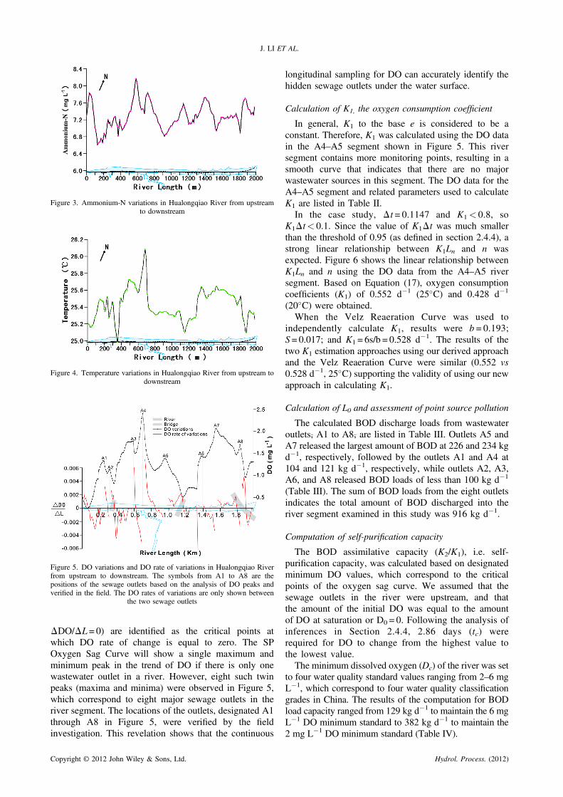
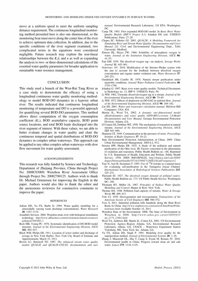


![Dissolved Oxygen [DO]](https://img.pdfslide.us/doc/110x75/5a6721977f8b9ab12b8b464b/dissolved-oxygen-do.jpg)