Monge Ampere Based Moving Mesh Methods for Weather Forecasting

Chris Budd (Bath)

Chiara Piccolo, Mike Cullen (Met Office)Emily Walsh (Bath,SFU), Phil Browne (Bath)

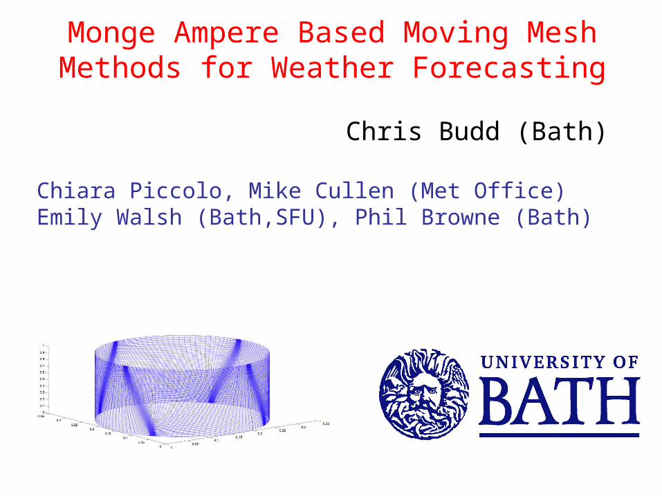
In NWP often need to locally refine a mesh to capture small scales

(i) For accurate numerical computation eg. Storms

(ii) For accurate assimilation of observed data to avoid spurious correlations

r-adaptive moving mesh methods aim to do this by the ‘optimal placement’ of a fixed number of mesh points which move during the computation

There are many advantages with r-adaptivity

• Constant data structures and mesh topology

• Ease of coupling to CFD solvers

• Capturing dynamical physics of the solution eg. Lagrangian behaviour, symmetries, conservation laws, self-similarity

• Global control of mesh regularityTraditional problems with r-adaptivity:

Mesh tangling, mesh skewness, implementation in 3D

Talk will describe an r-adaptive moving mesh method for doing this based upon geometrical ideas: optimal transport theory and Monge Ampere equations

Will demonstrate that this leads to a fast, robust and effective moving mesh method for adaptive NWP

• Which avoids mesh tangling and extreme skewness

• Works well in 2D and 3D

• Can be easily coupled to CFD solvers and DA codesH. Ceniceros and T Hou, J. Comp Phys (2001)CJB and J.F. Williams, Journal of Physics A, (2006)G.Delzano, L.Chacon, J. Finn, Y. Chung & G.Lapenta, J. Comp Phys (2008)CJB and J.F. Williams, SIAM J. Sci. Comp (2009) CJB, W-Z Huang and R.D. Russell, ACTA Numerica (2009)C.Kuhnlein, P.Smolarkiewicz and A.Dornbrack, J. Comp. Phys (2012)CJB, M.Cullen and E.Walsh, (2012) submitted

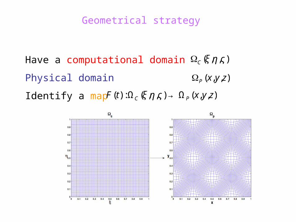
Geometrical strategy

Have a computational domain

Physical domain

Identify a map €

ΩC (ξ ,η ,ς )

€

ΩP (x, y,z)

€

F(t) : ΩC (ξ ,η ,ς ) → ΩP (x, y,z)

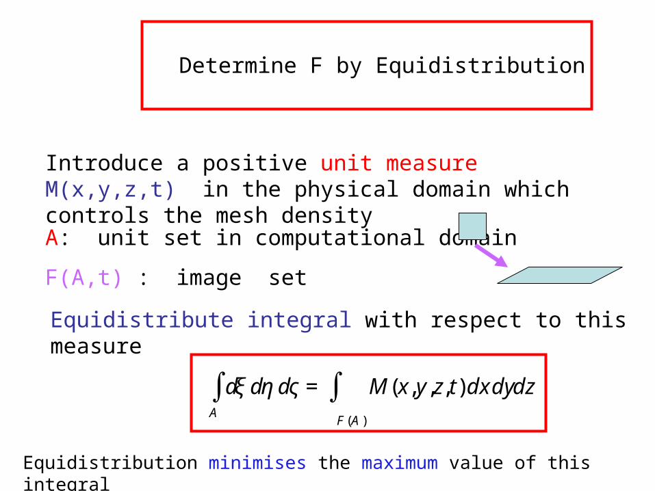
Determine F by Equidistribution

Introduce a positive unit measure M(x,y,z,t) in the physical domain which controls the mesh densityA: unit set in computational domain

F(A,t) : image set

€

dA

∫ ξ dη dς = M(x, y,z, t) dx dy

F (A )

∫ dz

Equidistribute integral with respect to this measure

Equidistribution minimises the maximum value of this integral

€

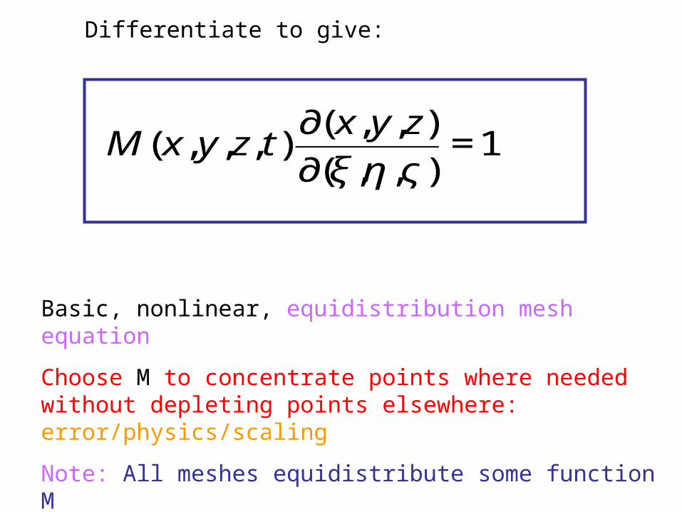
M(x, y,z, t)∂(x,y,z)

∂(ξ ,η ,ς )=1

Differentiate to give:

Basic, nonlinear, equidistribution mesh equation

Choose M to concentrate points where needed without depleting points elsewhere: error/physics/scaling

Note: All meshes equidistribute some function M

[Radon-Nicodym]

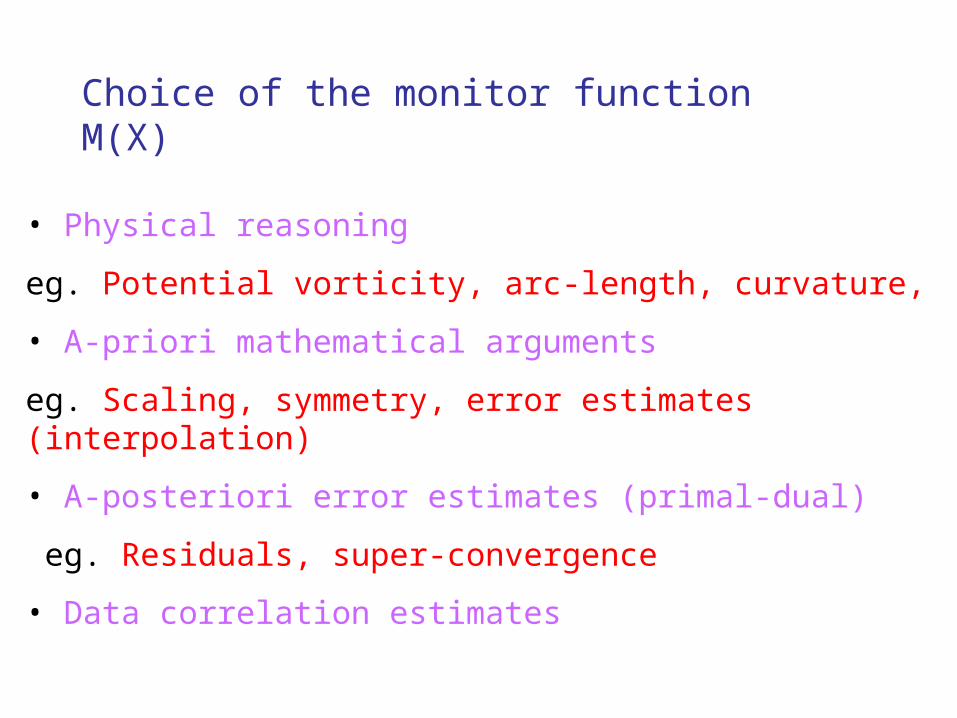
Choice of the monitor function M(X)

• Physical reasoning

eg. Potential vorticity, arc-length, curvature,

• A-priori mathematical arguments

eg. Scaling, symmetry, error estimates (interpolation)

• A-posteriori error estimates (primal-dual)

eg. Residuals, super-convergence

• Data correlation estimates

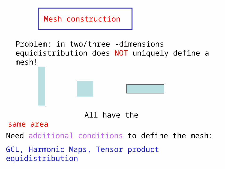
Mesh construction

Problem: in two/three -dimensions equidistribution does NOT uniquely define a mesh!

All have the same area

Need additional conditions to define the mesh:

GCL, Harmonic Maps, Tensor product equidistribution

F

),( ηξCΩ

€

ΩP (x, y)

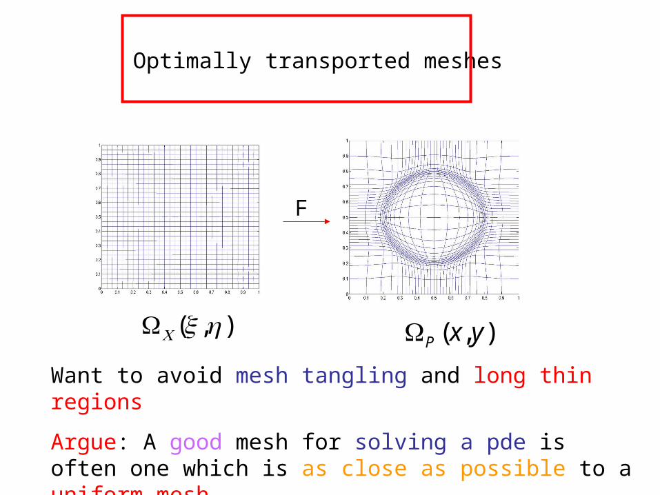
Optimally transported meshes

Want to avoid mesh tangling and long thin regions

Argue: A good mesh for solving a pde is often one which is as close as possible to a uniform mesh

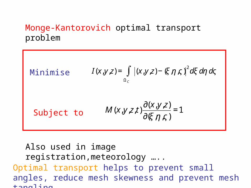
Monge-Kantorovich optimal transport problem

€

I(x, y,z) =ΩC

∫ (x,y,z) − (ξ ,η ,ς )2dξ dη dς

€

M(x, y,z, t)∂(x,y,z)

∂(ξ ,η ,ς )=1

Minimise

Subject to

Also used in image registration,meteorology …..

Optimal transport helps to prevent small angles, reduce mesh skewness and prevent mesh tangling.

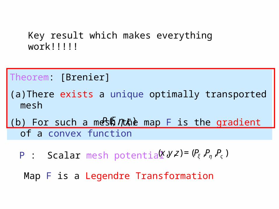
Key result which makes everything work!!!!!

Theorem: [Brenier]

(a)There exists a unique optimally transported mesh

(b) For such a mesh the map F is the gradient of a convex function

€

P(ξ ,η ,ς )

P : Scalar mesh potential

Map F is a Legendre Transformation

€

(x, y,z) = (Pξ ,Pη ,Pς )

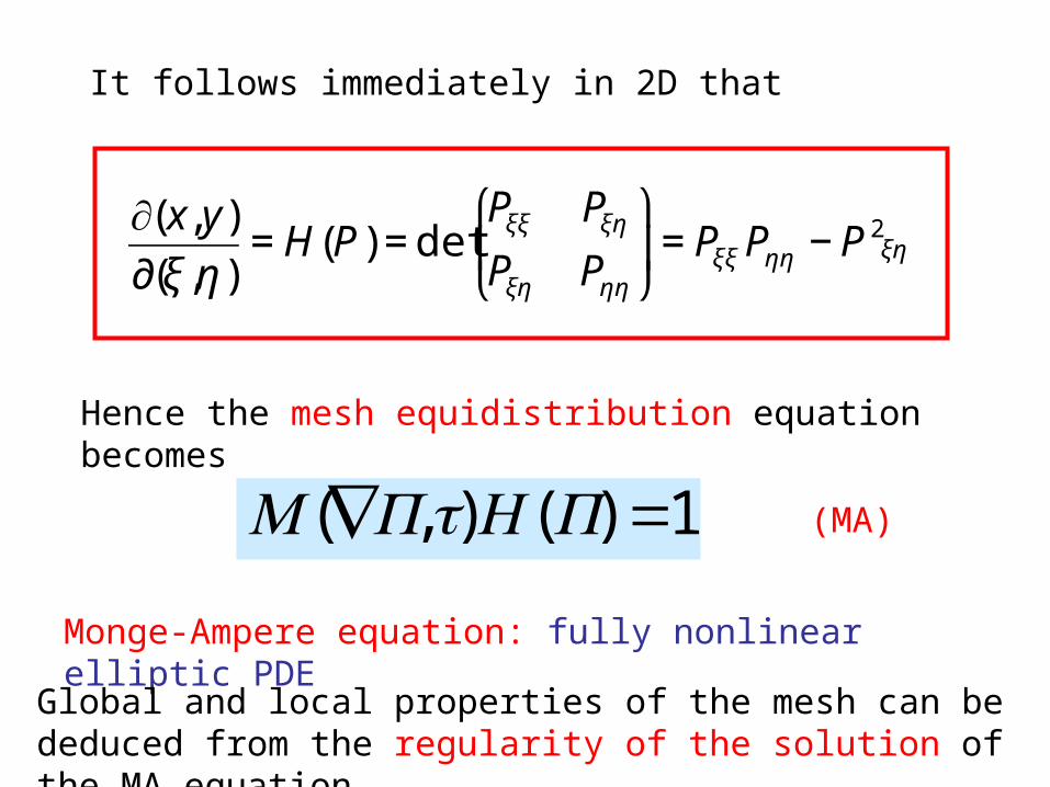
Monge-Ampere equation: fully nonlinear elliptic PDE

€

∂(x,y)

∂(ξ ,η )= H(P) = det

Pξξ Pξη

Pξη Pηη

⎛

⎝ ⎜

⎞

⎠ ⎟= Pξξ Pηη − P 2

ξη

1)(),( =∇ PHtPM

It follows immediately in 2D that

Hence the mesh equidistribution equation becomes

(MA)

Global and local properties of the mesh can be deduced from the regularity of the solution of the MA equation

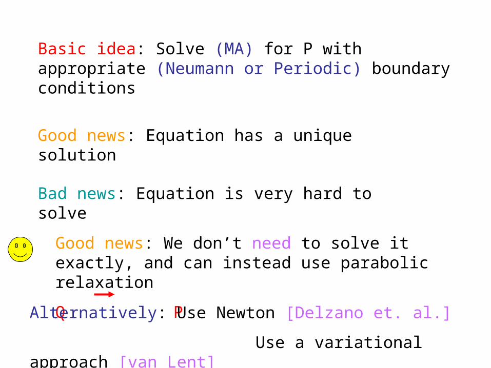
Basic idea: Solve (MA) for P with appropriate (Neumann or Periodic) boundary conditions

Good news: Equation has a unique solution

Bad news: Equation is very hard to solve

Good news: We don’t need to solve it exactly, and can instead use parabolic relaxation

Q PAlternatively: Use Newton [Delzano et. al.]

Use a variational approach [van Lent]

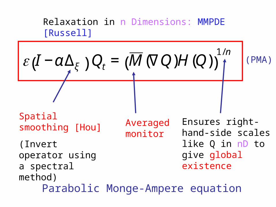
Relaxation in n Dimensions: MMPDE [Russell]

€

ε I −αΔξ( ) Qt = M (∇Q)H(Q)( )1/ n

Spatial smoothing [Hou]

(Invert operator using a spectral method)

Averaged monitor

Ensures right-hand-side scales like Q in nD to give global existence

Parabolic Monge-Ampere equation

(PMA)

Solution Procedure

If M is prescribed then the PMA equation can be discretised in the computational domain and solved using an explicit forward Euler method. This is a fast procedure: 5 mins for a 3D meteorological meshApplications

• Image processing and image registration

• Mesh generation for meteorological Data assimilation [Browne, CJB, Cullen, Piccolo]

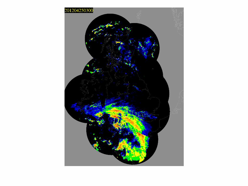
Take M to be a scaled approximation of the Potential Vorticity of the 3D flow

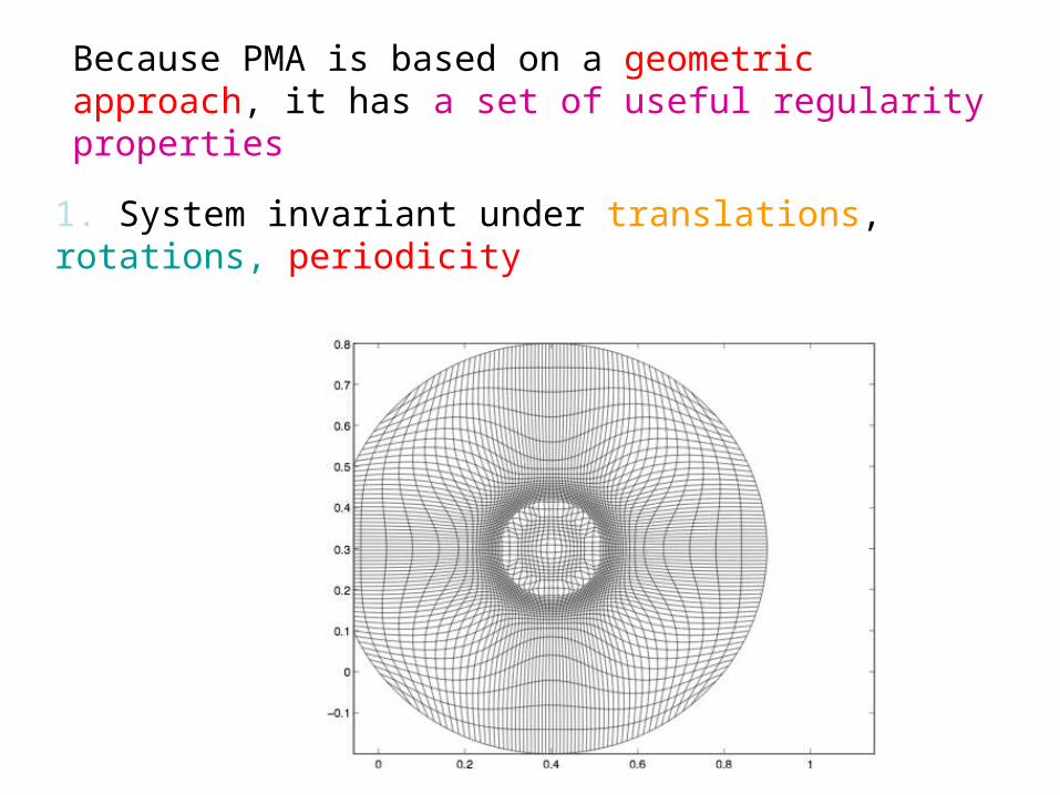
Because PMA is based on a geometric approach, it has a set of useful regularity properties

1. System invariant under translations, rotations, periodicity

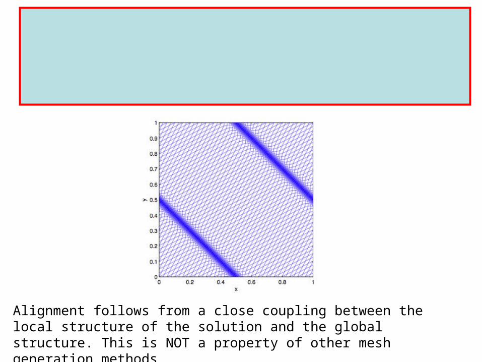
Lemma 1: CJB, EJW [2012]

The solutions of the MA equation exactly align with global linear features

Alignment follows from a close coupling between the local structure of the solution and the global structure. This is NOT a property of other mesh generation methods

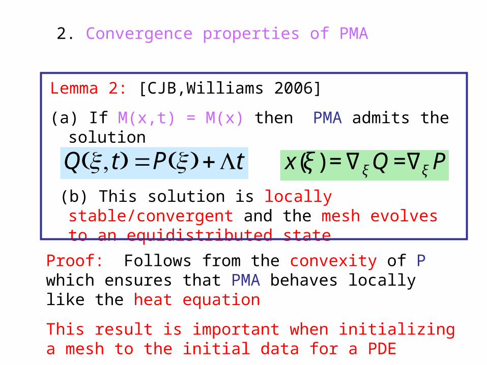
2. Convergence properties of PMA

Lemma 2: [CJB,Williams 2006]

(a) If M(x,t) = M(x) then PMA admits the solution

(b) This solution is locally stable/convergent and the mesh evolves to an equidistributed state

tPtQ Λ+= )(),( ξξ

€

x(ξ ) =∇ξ Q =∇ξ P

Proof: Follows from the convexity of P which ensures that PMA behaves locally like the heat equation

This result is important when initializing a mesh to the initial data for a PDE

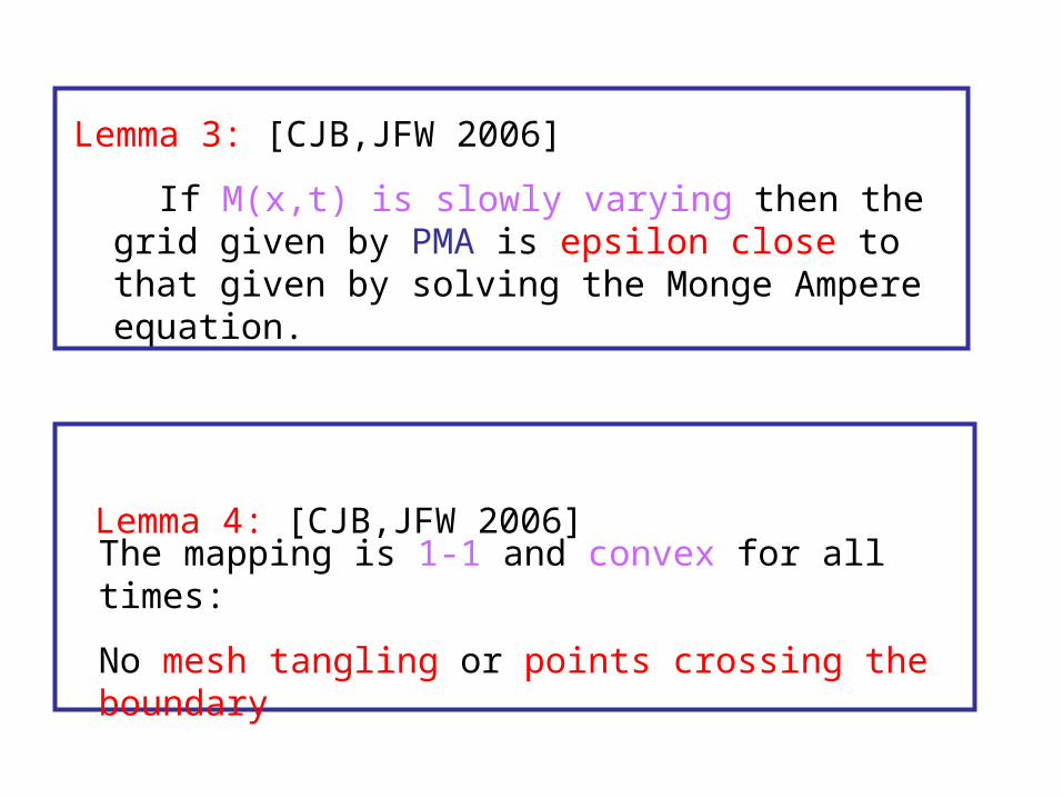
Lemma 3: [CJB,JFW 2006]

If M(x,t) is slowly varying then the grid given by PMA is epsilon close to that given by solving the Monge Ampere equation.

Lemma 4: [CJB,JFW 2006]The mapping is 1-1 and convex for all times:

No mesh tangling or points crossing the boundary

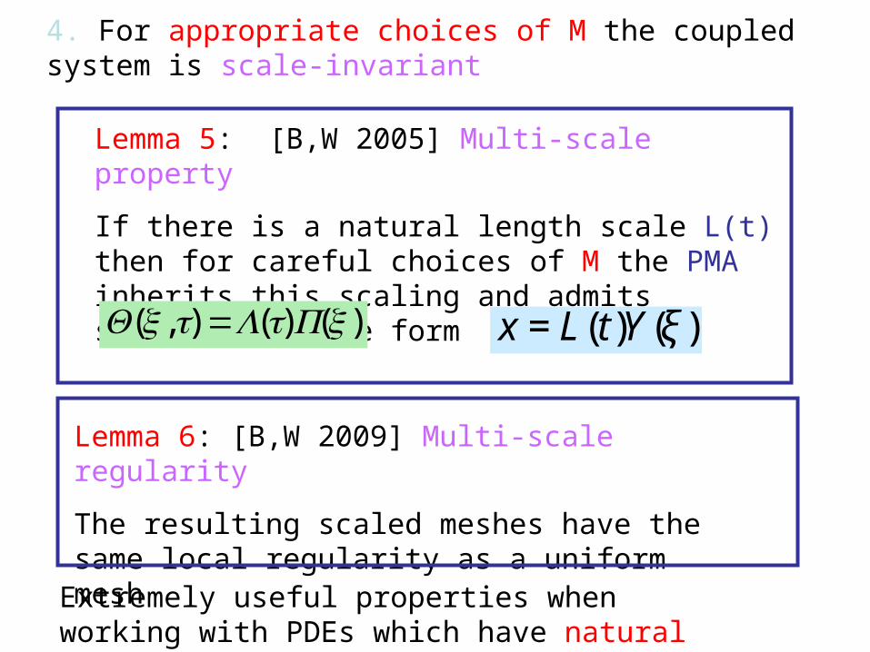
Lemma 5: [B,W 2005] Multi-scale property

If there is a natural length scale L(t) then for careful choices of M the PMA inherits this scaling and admits solutions of the form)()(),( ξξ PtLtQ =

€

x = L(t)Y (ξ )

Extremely useful properties when working with PDEs which have natural scaling laws

4. For appropriate choices of M the coupled system is scale-invariant

Lemma 6: [B,W 2009] Multi-scale regularity

The resulting scaled meshes have the same local regularity as a uniform mesh

Coupling to a PDE

More usually M is a function of the solution of a PDE and we must couple mesh generation to a CFD calculation

Carefully discretise PDE & PMA in the computational domain:

QuickTime™ and a decompressor

are needed to see this picture.

Solve the coupled mesh and PDE system either

Method One

As one large system (stiff!)

Velocity based Lagrangian approach. Works well for parabolic blow-up type problems (JFW)

Advantages:

No need for interpolation

Mesh and solution become one large dynamical system and can be studied as such

Disadvantage: Equations are very hard to solve especially when the PDE is strongly advective

Method 2: More suitable for metorology

By alternating between evolving the PDE and mesh

1. Time march the PDE on given mesh

2. Evolve to new mesh by solving PMA to steady state

3. Interpolate PDE solution onto the new mesh

4. Repeat from 1.

Advantages:

Very flexible, can build in conservation laws and incompressibility at stage 2

Disadvantage: Interpolation is difficult and expensive

€

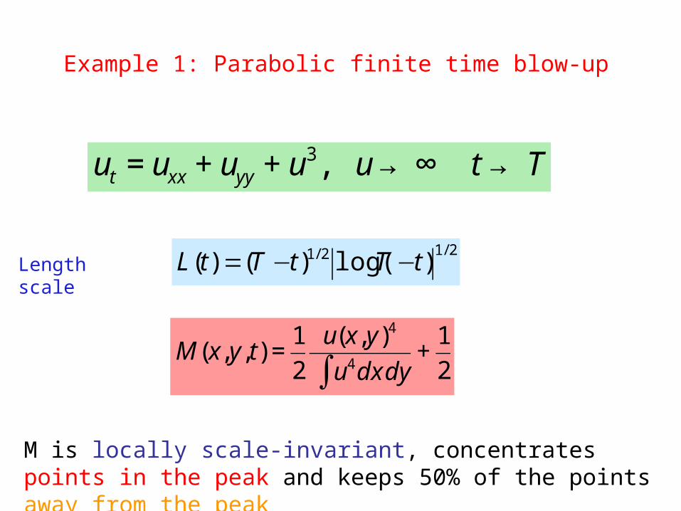
ut = uxx + uyy + u3, u → ∞ t → T

2/12/1 )log()()( tTtTtL −−=

€

M(x,y, t) =1

2

u(x, y)4

u4∫ dx dy+

1

2

Example 1: Parabolic finite time blow-up

M is locally scale-invariant, concentrates points in the peak and keeps 50% of the points away from the peak

Length scale

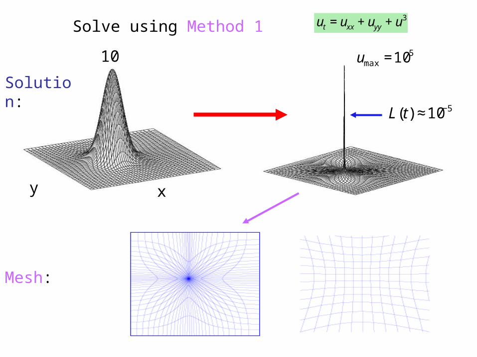
Solve using Method 1

€

ut = uxx + uyy + u3

Mesh:

Solution:

xy

10

€

umax =105

€

L(t) ≈10−5

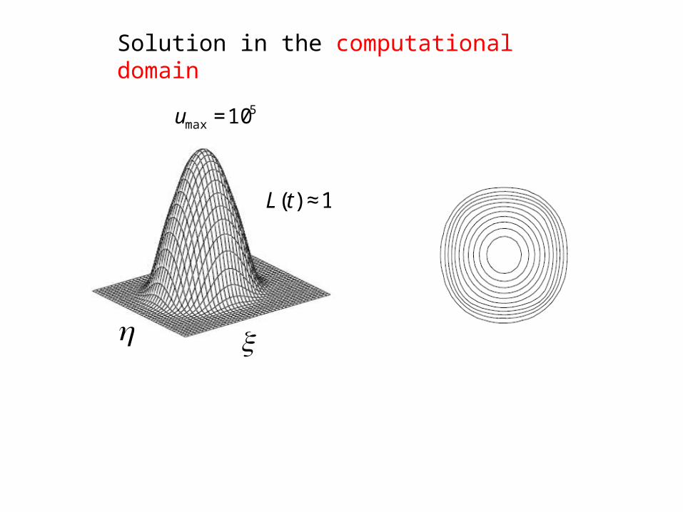
Solution in the computational domain

ξη

€

umax =105

€

L(t) ≈1

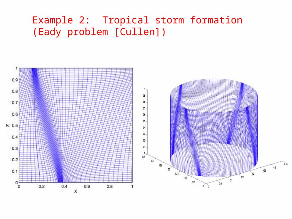
Example 2: Tropical storm formation (Eady problem [Cullen])

QuickTime™ and a decompressor

are needed to see this picture.

Conjectured discontinuity singularity after t = 6.3 days

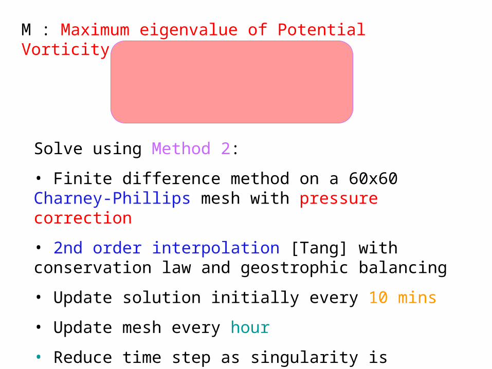
Solve using Method 2:

• Finite difference method on a 60x60 Charney-Phillips mesh with pressure correction

• 2nd order interpolation [Tang] with conservation law and geostrophic balancing

• Update solution initially every 10 mins

• Update mesh every hour

• Reduce time step as singularity is approached

€

R=f 2 + f vx f vz

gθ0−1θx gθ0θ z

⎛

⎝ ⎜

⎞

⎠ ⎟

M : Maximum eigenvalue of Potential Vorticity R

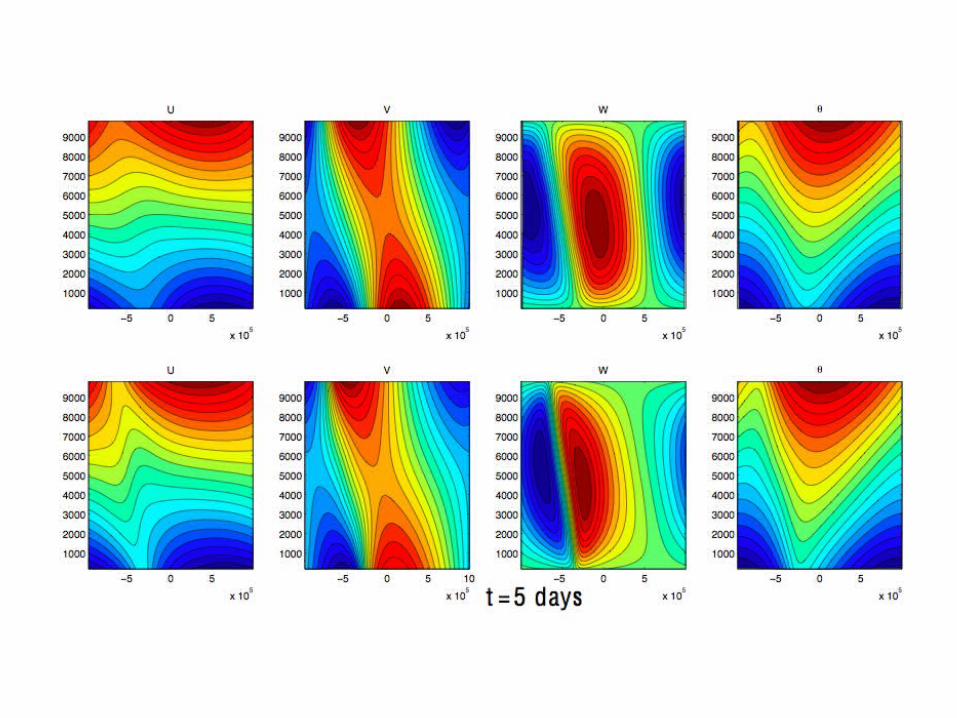
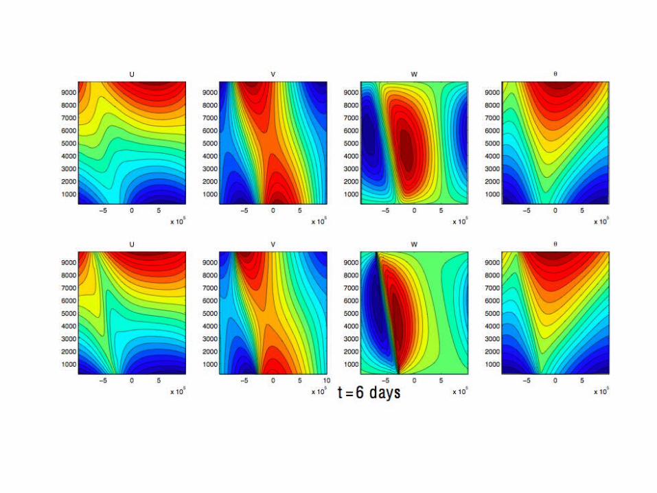
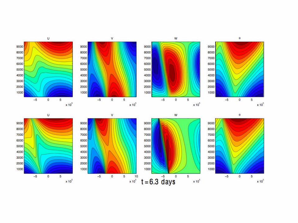
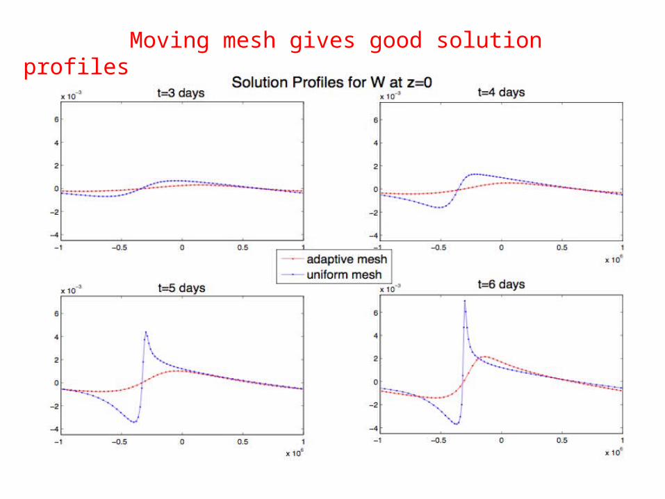
Moving mesh gives good solution profiles

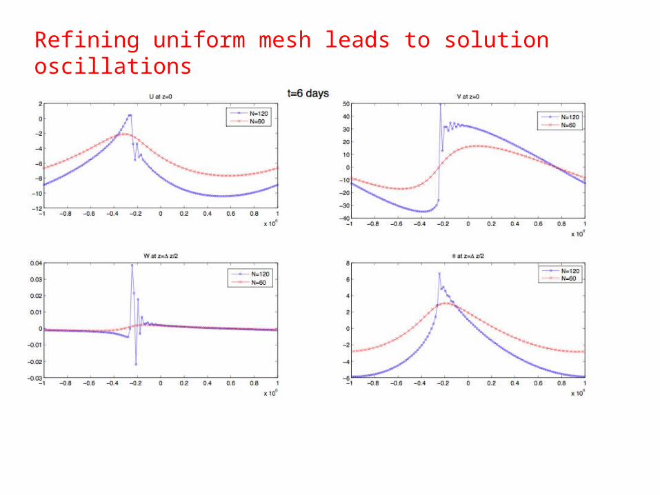
Refining uniform mesh leads to solution oscillations

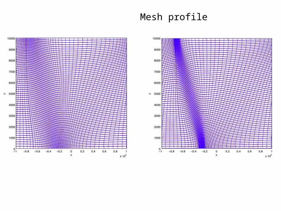
Mesh profile

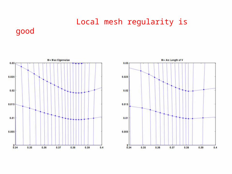
Local mesh regularity is good

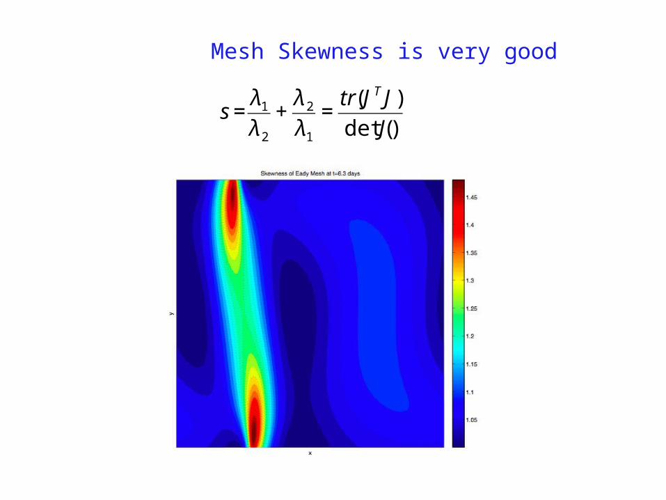
Mesh Skewness is very good

€

s =λ1

λ 2

+λ 2

λ1

=tr(JT J)

det(J)

Conclusions

• Optimal transport is a natural way to determine moving meshes in dimensions greater than one

• It can be implemented using a fast relaxation process by using the PMA algorithm

• Method works well for a variety of problems, and there are rigorous estimates about its behaviour

• Looking good on meteorological problems

• Lots of work to do to compare its effectiveness with tried and tested AMR procedures on standard test problems

• Maybe a good project for the INI programme?