Pertanika.J. Soc. Sci & Hum. 1(1): 81-90 (1993) ISSN: 0128-7702© Universiti Pertanian Malaysia Press

Money and Biased Technical Progress: A Further. Test on'Monetization as Technological Innovation' Hypothesis

MUZAFAR SHAH HABIBULLAHDepartment of Economics, Faculty of Economics and Management,

Universiti Pertanian Malaysia,

43400 UPM Serdang, Selangor Daml Ehsan, Malaysia.

Keywords: Money, biased technical progress, 'monetization as technological innovation'

ABSTRAK

Kajian-kajian laiu telah menguji hipotesis 'pengewangan merupakan inovasi teknologi' untuk negara India.Oleh itu, tujuan artikel ini adalah untuk menguji hipotesis di atas terhadap data sektor estet getah di Malaysia,untuk tempoh masa 1962-89. Artikel ini juga ingin menentukan bias perubahan teknikal terhadap buruh danmodal di dalam sektor estet getah. Di dalam kajian ini, kaedah fungsi pengeluaran konvensional dan modelpembetulan ralat (error correction model) digunakan untuk analisis. Keputusan kajian menyarankan bahawajumlah bias di dalam perubahan teknikal adalah mem~u ke arah penjimatan buruh. Juga, hasil kajian inimendapati bahawa kegagalan untuk mengambilkira ketakpegunan sesuatu pembolehubah di dalampenganggaran akan menyebabkan kepada penganggaran yang tertakluk kepada bias-keatas yang agak besar.

ABSTRACT

Recent studies have tested the hypothesis of 'monetization as technological innovation' for the Indianeconomy. The objective of this paper is to test the above hypothesis on the the Malaysian rubber estate sectordata over the period 1962-89. We seek to determine the bias in technical change on labor and capital in therubber estate sector economy. In this study, we use both the conventional and the error correction model ofproduction function. Results indicate that the lOtal bias in technical change is labor saving. The study funherpoints out that the failure to appropriately allow for non-stationary il1legrated variables in estimation has led lOestimates which are subjected to substantial upward bias.

INTRODUCTION

Traditionally in production, output has beenspecified as a function of capital and labor. Thistechnical relationship between output and inputhas been recognised by economists for over half acentury. More recently, Sinai and Stokes (1972)provided empirical evidence which suggests thatreal money balances is a third factor input in theproduction function. However, the role of moneyas a factor input, has been recognised in earlierIi terature by Friedman (1959, 1969), Bailey(1971), Johnson (1969), Levhari and Patinkin(1968), Moroney (1972) and Nadiri (1969).

Despite the pioneering work done by Sinaiand Stokes (1972), the consideration of realmoney balances as a production input has beencriticised by Fischer (1974), iccoli (1975), Prais(1975a, 1975b), Khan and Kouri (1975), Ben­Zion and Ruttan (1975) and Boyes andKavanaugh (1979). They argue that Ill­

corporating real money balances in the

production function is subjected to aspecification bias.

Nevertheless, recent empirical evidence bySimos (1981), Apostolakis (1983), You (1981),Short (1979), Subrahmanyam (1980), Khan andAhmad (1985), and Sarwar et at. (1989) havestrongly supported the idea that real moneybalances act as a productive input in production.The reason for incorporating real moneybalances as a factor of production is that realmoney balances is a medium of exchange andfacilitates the exchange between capital andlabor for specialisation purposes, and tends toincrease productivity. Also, it tends to reduce thetransaction cost and therefore, increases theeconomic efficiency of the money market system.Thus, money acts as an input augmenting factorof production.

In two recent papers, Subrahmanyam andCosimano (1979) (hereafter S-C) have tested the'monetization as technological innovation'

Muzafar Shah Habibullah

hypothesis, using data from the Indian economyby employing the CES production functionframework. The study by S-C found that totaltechnical change has been biased in the capitalsaving direction. In examining the bias due totime and the bias due to real money balancesseparately, S-C found that real money balancesare biased toward labor saving, and that capitalsaving is biased toward time. On the other hand,Gupta (1985) using the translog cost functionapproach in testing the 'monetization astechnological innovation' hypothesis for theIndian economy, found that his results contradictthe earlier findings by S-C. Gupta (1985) pointsout that total technical change has been biasedtoward labor saving, and further, both time andreal money balances lead to labor savingtechnological innovations.

The main objective of this paper is to test the'monetization as technological innovation'hypothesis based on Malaysian rubber estatesector data for the period 1962-1989. The paperis divided into four sections. The model used inthe study is discussed in Section 2. Empiricalresults are presented in Section 3, and the lastSection contains our conclusion.

THE MODEL

The term 'monetization as a technologicalinnovation' was coined by Crouch (1973) in hisstimulating seminal paper (see also Moroney1972). Crouch points out that on monetizing abarter economy, labor effort devoted in produc­tion that is, monetization of augmented laborinput in production is eliminated. Therefore, heargues that in production function, monetizationis equivalent to a one-shot labor augmentingtechnological innovation. With the introductionof money, the benefits are reaped all at once andthat, the productive labor force is increased by acertain factor. The larger the benefits reapedfrom monetization, the larger will be thatparticular factor. Crouch further points thatwhen we view 'monetization as a technologicalinnovation,' it must lead unambiguously tohigher income, wage rate and capital-labor ratio.

In this study, we employ the approach givenby Subrahmanyam and Cosimano (1979) inorder to test the 'monetization as a technologicalinnovation' hypothesis. The S-C model is derivedfrom the neo-classical production function, in theCES form as follows

Q, [{I - 0} !aM~ exp (Qt) LT' + 0 lbM~ exp{m} K, I -T'/P (1)

where Q, M, Land K are output, real moneybalances, labor and capital respectively. a and ~

are elasticities of efficiency of a and b with respectto M respectively. Q and 1t are time rate of laborand capital augmenting technical changerespectively. 0, a, band p are parameters, and t isthe time period.

Assuming cost minimization, and equatingthe marginal products of the inputs to theirrespective prices, and after taking logarithms wearrive at the follO\ving relation

log (K/L) , = log ((a/b)" [0/ (1- 0)] 1+ crlog(w/r), + [(1 - cr) (a - B) ]log M, +[(1- 0-) (Q -1t)]t (2)

where cr is the elasticity of capital-laborsubstitution. And defining Equation (2) incompact form and after adding a stochastic termwe have Equation (3) which is ready forestimation.

log (K/L), =t" + t,log (w/r) ,H,log M, + t,t + E, (3)

where ~ is the disturbance term, assumed to havemean zero and constant variance.

Our main focus is to measure the total biasin technical change, and separate biases due toreal money balances and time. It has been shownthat, using the results from Equation (3), themeasurement of total bias in technical progresscan be calculated as follows (see for example;Amano, 1964; Dandrakis and Phelps, 1966; Davidand Kundert, 1965; Subrahrnanyam andCosimano,1979),

B=[(~-a)m+(n-Q)][cr-(1/cr)] (4)

or calculated from the estimating Equation (3) as

B = Ht/(1- t,)]m -[t/(1- t,)]I[(t,-l)tJ (5)

where B is the measure of total bias in technicalprogress and m is the rate of growth of realmoney balances. If B > 0, we have total bias inlabor saving. If B < 0, we have total bias in capitalsaving, and if B = 0, we have neutral technicalprogress.

The biases due to real money balances(a - ~) and time (Q - 1t) are shown by the terms

82 PertanikaJ. Soc. Sci. & Hum. Vol. I No. I 1993

Money and Biased Technical PI'ogress

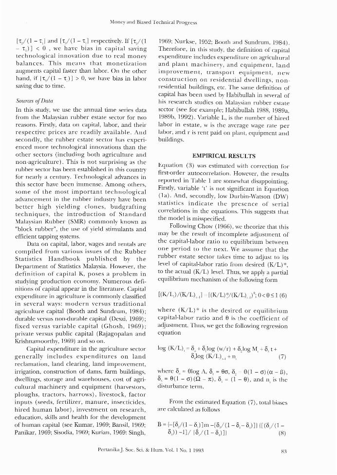
['2/(1 - 'I] and [,/(1 - 'I] respectively. If [,/(1- 'I)] < °,we have bias in capital savingtechnological innovation due to real moneybalances. This means that monetizationaugments capital faster than labor. On the otherhand, if ['/ (1 - ,)] > 0, we have bias in laborsaving due to time.

Sow'ces ofData

In this study, we use the annual time series datafrom the Malaysian rubber estate sector for tworeasons. Firstly, data on capital, labor, and theirrespective prices are readily available. Andsecondly, the rubber estate sector has experi­enced more technological innovations than theother sectors (including both agriculture andnon-agriculture). This is not surprising as therubber sector has been established in this countryfor nearly a century. Technological advances inthis sector have been immense. Among others,some of the most important technologicaladvancement in the rubber industry have beenbetter high yielding clones, budgraftingtechniques, the introduction of StandardMalaysian Rubber (SMR) commonly known as"block rubber", the use of yield stimulants andefficien t tapping systems.

Data on capital, labor, wages and rentals arecompiled from various issues of the RubberStatistics Handbook published by theDepartment of Statistics Malaysia. However, thedefinition of capital K, poses a problem instudying production economy. umerous defi­nitions of capital appear in the literature. Capitalexpenditure in agriculture is commonly classifiedin several ways: modern versus traditionalagriculture capital (Booth and Sundrum, 1984);durable versus non-durable capital (Desai, 1969);fixed versus variable capital (Ghosh, 1969);private versus public capital (Rajagopalan andKrishnamoorthy, 1969) and so on.

Capital expenditure in the agriculture sectorgenerally includes expenditures on landreclamation, land clearing, land improvement,irrigation, construction of dams, farm buildings,dwellings, storage and warehouses, cost of agri­cultural machinery and equipment (harvestors,ploughs, tractors, harrows), livestock, factorinputs (seeds, fertilizer, manure, insecticides,hired human labor), investment on research,.education, skills and health for the developmentof human capital (see Kumar, 1969; Bansil, 1969;Panikar, 1969; Sisodia, 1969; Kurian, 1969: Singh,

1969; urkse, 1952; Booth and Sundrum, 1984).Therefore, in this study, the definition of capitalexpenditure includes expenditure on agriculturaland plant machinery, and equipment, landimprovement, transport equipment, newconstruction on residential dwellings, non­residential buildings, etc. The same definition ofcapital has been used by Habibullah in several ofhis research studies on Malaysian rubber estatesector (see for example; Habibullah 1988, 1989a,1989b, 1992). Variable L, is the number of hil-edlabor in estate, w is the average wage rate perlabor, and r is rent paid on plant, equipment andbuildings.

EMPIRlCAL RESULTS

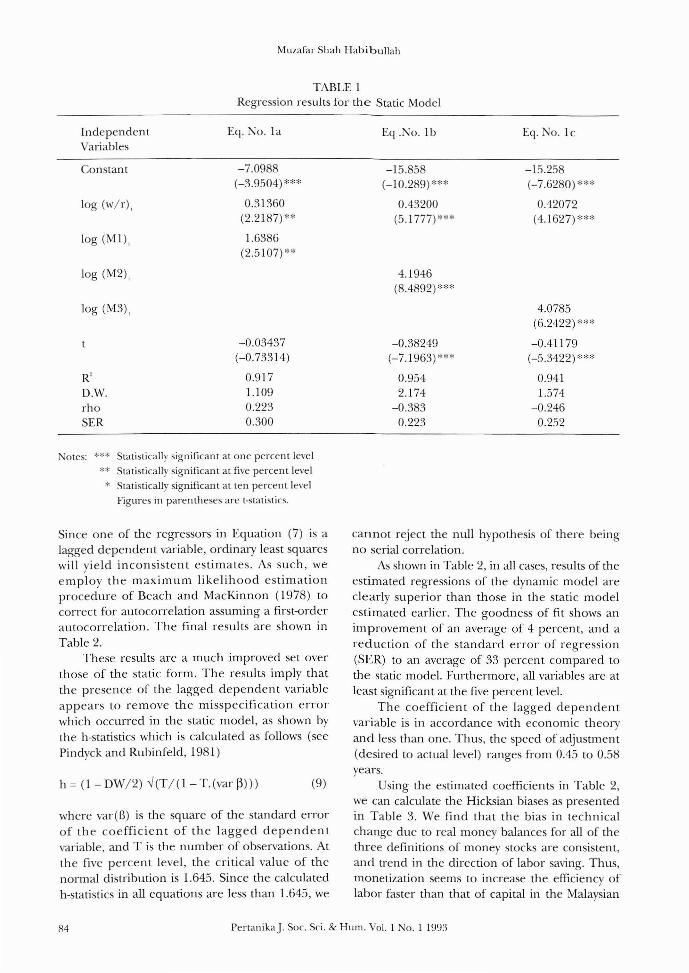
Equation (3) was estimated with correction forfirst-order autocorrelation. However, the resultsreported in Table 1 are somewhat disappointing.Firstly, variable 't' is not significant in Equation(la). And, secondly, low Durbin-Watson (DW)statistics indicate the presence of serialcorrelations in the equations. This suggests thatthe model is misspecified.

Following Chow (1966), we theorize that thismay be the result of incomplete adjustment ofthe capi tal-labor ratio to equilibrium betweenone period to the next. We assume that therubber estate sector takes time to adjust to itslevel of capital-labor ratio from desired (K/L) 0(.,

to the actual (K/L) level. Thus, we apply a partialequilibrium mechanism of the following form

[(K/L)/(K/L),_I] = [(K/L)j(K/Ltl; 0<8 ~ 1 (6)

where (K/L) 0(. is the desired or equilibriumcapital-labor ratio and 8 is the coefficient ofadjustment. Thus, we get the following regressionequation

log (K/L), =b" + b1log (w/r) + b)og M, + b, t +b)og (K/L)'_I + n, (7)

where 0" = 810g A, bl = 80, b" = 8(1- 0) (a. - B),b, = 8(1 - 0) (Q - IT), 01= (1- - 8), and n, is thedisturbance term.

From the estimated Equation (7), total biasesare calculated as follows

B = {-[O/(1- OJ]m -[0/ (1 - b,- 0')] II [(b/ (1 -b,)) -1]1 [b/(1- 0,)]1 (8)

PertanikaJ. Soc. Sci. & Hum. Vol. I No. I 1990l SOl

Muzafar Shah Habibullah

TABLE IRegression results for the Static Model

Independent Eg. No. laVariables

Constant -7.0988(-3.9504) ***

log (w/r), 0.31360(2.2187) **

log (MI), 1.6386(2.5107) **

log (M2),

log (M3),

-0.03437(-0.73314)

R' 0.917D.W. 1.l09rho 0.223SER 0.300

Eg.l o. Ib

-15.858(-10.289)***

0.43200(5.1777) ***

4.1946(8.4892) ***

-0.38249(-7.1963)***

0.9542.174

-0.3830.223

Eg. No. lc

-15.258(-7.6280)***

0.42072(4.1627) ***

4.0785(6.2422) ***

-0.41179(-5.3422) *"'*

0.9411.574

-0.2460.252

Notes: *':'* Statistically significant at one percent level

** Statistically significant at five percent level

* Statistically significant at ten percent level

Figures in parentheses are t-statistics.

where var(f3) is the square of the standard errorof the coefficient of the lagged dependentvariable, and T is the number of observations. Atthe five percent level, the critical value of thenormal distribution is 1.645. Since the calculatedh-statistics in all equations are less than 1.645, we

Since one of the regressors in Equation (7) IS alagged dependent variable, ordinary least squareswill yield inconsistent estimates. As such, weemploy the maximum likelihood estimationprocedure of Beach and MacKinnon (1978) tocorrect for autocorrelation assuming a first-orderautocorrelation. The final results are shown inTable 2.

These results are a much improved set overthose of the static form. The results imply thatthe presence of the lagged dependent variableappears to remove the misspecification errorwhich occurred in the static model, as shown bythe h-statistics which is calculated as follows (seePindyck and Rubinfeld, 1981)

h = (1- DW/2) --J(T/(I- T.(var ~)) (9)

cannot reject the null hypothesis of there beingno serial correlation.

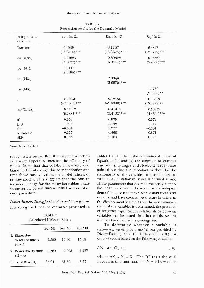
As shown in Table 2, in all cases, results of theestimated regressions of the dynamic model areclearly superior than those in the static modelestimated earlier. The goodness of fit shows animprovement of an average of 4 percent, and areduction of the standard error of regression(SER) to an average of 33 percent compared tothe static model. Furthermore, all variables are atleast significant at the five percent level.

The coefficient of the lagged dependentvariable is in accordance with economic theoryand less than one. Thus, the speed of adjustment(desired to actual level) ranges from 0.45 to 0.58years.

Using the estimated coefficients in Table 2,we can calculate the Hicksian biases as presentedin Table 3. We find that the bias in technicalchange due to real money balances for all of thethl-ee definitions of money stocks are consistent,and trend in the direction of labor saving. Thus,monetization seems to increase the efficiency oflabor faster than that of capital in the Malaysian

84 PertanikaJ. Soc. Sci. & Hum. Vol. I No.1 1993

Money and Biased Technical Progress

TABLE 2Regression results for the Dynamic Model

IndependentVariables

Eg. No. 2a Eg. No. 2b Eg. No 2c

Constant

log (w/r),

log (M!),

-5.0840(-3.9515)***

0.27693(3.5827) ***

1.3147(3.0395)***

-8.1167(-3.3675) ***

0.39628(6.0441)***

-6.4817(-2.7717)***

0.38667(5.4620) ***

log (M2), 2.0046(2.8672) ***

log (M3),

log (K/L)'_l

R'D.W.rhoh-statisticSER

-0.06656(-2.7767)***

0.54313(6.2882) ***

0.9761.904

-0.3340.2770.166

-0.18436(-2.8088)***

0.41817(3.4128) ***

0.9752.148

-0.327-0.468

0.169

1.5760(2.2506) **

-0.16369(-2.1829) **

0.50957(4.4604) ***

0.9741.714

-0.2310.8710.175

ate: As per Table 1

TABLE 3Calculated Hicksian Biases

Further Analysis: Testingfor Unit Roots and Cointegmtion

It is recognised that the estimates presented in

1. Biases dueto real balances 7.306 10.80 15.19(a.-il)

2. Biases due to time -0.369 -0.993 -1.577(Q - n)

rubber estate sector. But, the exogenous techni­cal change appears to increase the efficiency ofcapital faster than that of labor. However, totalbias in technical change due to monetization andtime shows positive values for all definitions ofmoney stocks. This suggests that the bias intechnical change for the Malaysian rubber estatesector for the period 1962 to 1989 has been laborsaving in nature.

(10)!'!, X, = a + pX'_l + e,

where !'!,X, = X, - X'_l.The DF tests the nullhypothesis of a unit root, Ho: X, '" I (1), which is

Tables 1 and 2, from the conventional model ofEquations (l) and (3) are subjected to spuriousregressions. Granger and Newbold (1977) havepointed out that it is important to check for thestationarity of the variables in question beforeestimation. A stationary series is defined as onewhose parameters that describe the series namelythe mean, variance and covariance are indepen­dent of time, or rather exhibit constant mean andvariance and have covariances that are invariant tothe displacement in time. Once the non-stationarystatus of the variables is determined, the presenceof long-run equilibrium relationships betweenvariables can be tested. In other words, we testwhether the variables are cointegrated.

To determine whether a variable isstationary, we employ a useful test provided byDickey-Fuller (1979). The Dickey-Fuller (DF) teston unit root is based on the following equation

46.7752.5035.04

For Ml For M2 For M3

3. Total Bias (B)

PertanikaJ. Soc. Sci. & Hum. Vol. 1 No.1 1993 85

Muzafar Shah Habibullah

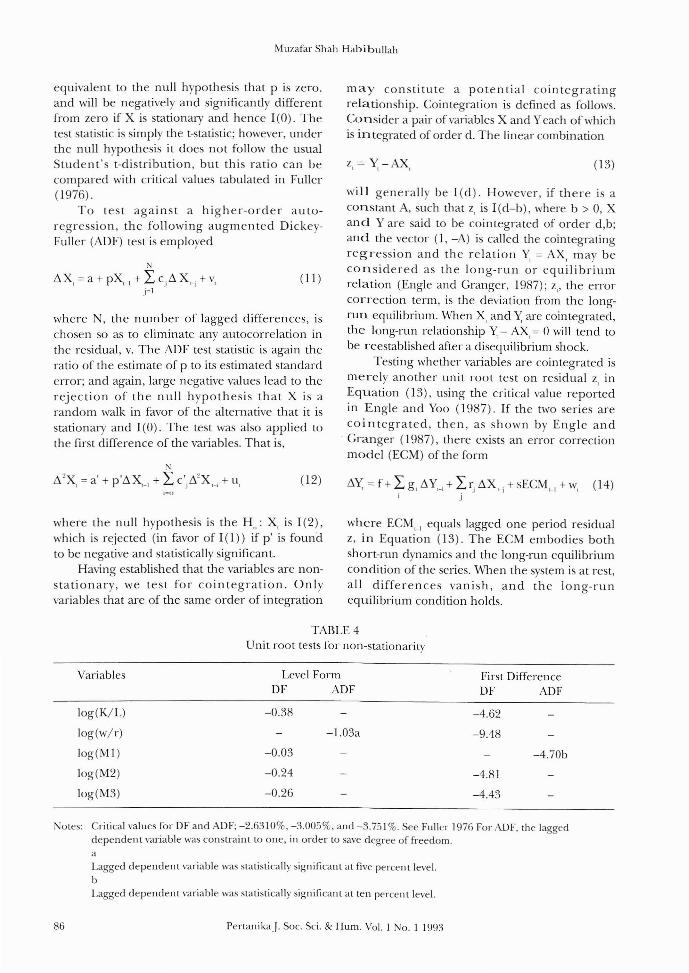
where N, the number of lagged differences, ischosen so as to eliminate any autocorrelation inthe residual, v. The ADF test statistic is again theratio of the estimate of p to its estimated standarderror; and again, large negative values lead to therejection of the null hypothesis that X is arandom walk in favor of the alternative that it isstationary and 1(0). The test was also applied tothe first difference of the variables. That is,

equivalent to the null hypothesis that p is zero.and will be negatively and significantly differentfrom zero if X is stationary and hence 1(0). Thetest statistic is simply the t-statistic; however, underthe null hypothesis it does not follow the usualStudent's t-distribution, but this ratio can becompared with critical values tabulated in Fuller(1976).

To test against a higher-order auto­regression, the following augmented Dickey­Fuller (ADF) test is employed

may constitute a potential cointegratingrelationship. Cointegration is defined as follows.Consider a pair of variables X and Yeach of whichis integrated of order d. The linear combination

will generally be I(d). However, if there is aconstant A, such that z, is I (d-b), where b > 0, Xand Yare said to be cointegrated of order d,b;and the vector (1, -A) is called the cointegratingregression and the relation Y, = AX, may beconsidered as the long-run or equilibriumrelation (Engle and Granger, 1987); z" the errorcorrection term, is the deviation from the long­run equilibrium. When X, and X are cointegrated,the long-run relationship X - AX, = 0 will tend tobe reestablished after a disequilibrium shock.

Testing whether variables are cointegrated ismerely another unit root test on residual z, inEquation (I3), using the critical value reponedin Engle and Yoo (I987). If the two series arecoin tegrated, then, as shown by Engle and

. Granger (1987), there exists an error correctionmodel (ECM) of the form

(13)z == Y-AX, , ,

(II)'J

t. X, = a + pX'_1 + L cit. X'_l + v,i"!

:\

t.'X =a'+p't.X I + Lc'.t.'X .+uI (- . I t-l I

(I2) t.X == f + L g; t. Y,_; + Ir; t.X'_i + sECM'_1 + w, (14)i j..

where the null hypothesis is the H,,: X, is 1(2),which is rejected (in favor of I (I)) if p' is foundto be negative and statistically significant.

Having established that the variables are non­stationary, we test for cointegration. Onlyvariables that are of the same order of integration

where ECM'_1 equals lagged one period residualz, in Equation (13). The ECM embodies bothshan-run dynamics and the long-run equilibriumcondition of the series. When the system is at rest,all differences vanish, and the long-runequilibrium condition holds.

TABLE 4Unit root tests for non-stationarity

Variables Level FormOF ADF

First DifferenceOF ADF

log(K/L)

log(w/r)

10g(MI)

log(M2)

log(M3)

-0.38

-1.03a

-0.03

-0.24

-0.26

-4.62

-9.48

-4.70b

-4.81

-4.43

otes: Critical values for OF and ADF; -2.6~ 10%, -3.005%, and -3.751 %. See Fuller 1976 For ADF, the laggeddependent variable was constraint to one, in order to save degree of freedom.

aLagged dependent variable was statistically significant at five percent level.

bl.agged dependent variable was statistically significant at ten percent level.

86 PertanikaJ. Soc. Sci. & Hum. Vol. 1 No. I 1993

Money and Biased Technical Progress

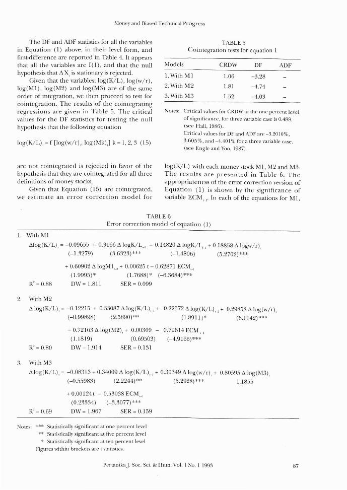
The OF and ADF statistics for all the variablesin Equation 0) above, in their level form, andfirst-difference are reported in Table 4. It appearsthat all the variables are 10), and that the nullhypothesis that L1 X, is stationary is rejected.

Given that the variables; 10g(K/L), log(w/r),10g(Ml), log(M2) and log(M3) are of the sameorder of integration, we then proceed to test forcointegration. The results of the cointegratingregressions are given in Table 5. The criticalvalues for the OF statistics for testing the nullhypothesis that the following equation

10g(K/L), =f [log(w/r)" log(Mk),] k =1,2,3 (15)

are not cointegrated is rejected in favor of thehypothesis that they are cointegrated for all threedefinitions of money stocks.

Given that Equation (15) are cointegrated,we estimate an error correction model for

TABLE 5Cointegration· tests for equation 1

Models CROW OF ADF1. With Ml 1.06 -3.28

2. With M2 1.81 -4.74

3. With M3 1.52 -4.03

Notes: Critical values for CRDW at the one percent levelof significance, for three variable case is 0.488.(see Hall, 1986).Critical values for DF and ADF are -3.2010%,3.605%, and -4.401 % for a three variable case.(see Engle and Yoo, 1987).

10g(K/L) with each money stock Ml, M2 and M3.The results are presented in Table 6. Theappropriateness of the error correction version ofEquation (1) is shown by the significance ofvariable ECM'_I. In each of the equations for Ml,

TABLE 6Error correction model of equation (1)

1. With Ml

Lilog(K/L), = -0.09655 + 0.3166 L1logK/L,_, - 0.14820 Li !ogK/L'-4 + 0.18858 Li logw/r),

(-1.3279) (3.6323)*** (-1.4806) (5.2702)***

R' = 0.88

+ 0.60902 Li logMl,_, + 0.00625 t - 0.62871 ECM'_I

(1.9995)* (1.7688)* (-6.3684)***

OW = 1.811 SER = 0.099

2. With M2

Li log(K/L), = -0.12215 + 0.33087 Li !og(K/L)'_1 + 0.22572 Li log(K/L),_, + 0.29858 Li log(w/r),

(-0.99898) (2.5890)** (1.8911)* (6.1142)***

R' = 0.80

+ 0.72163 Li log(M2), + 0.00309, -

(1.1819) (0.69503)

OW = 1.914 SER = 0.131

0.79614 ECM,-I

(-4.9166)***

3. With M3

Li 10g(K/L), = -0.08313 + 0.34009 Li log(K/L)'_1 + 0.30349 Li log(w/r), + 0.80595 Li ]og(M3),

(-0.55983) (2.2244) ** (5.2928) *** 1.1855

R' = 0.69

+ 0.00124t - 0.53038 ECM'_I

(0.23334) (-3.30nr'**

OW = 1.967 SER = 0.159

Notes: *** Statistically significant at one percent level,":' Statistically significant at five percent level* Statistically significant at ten percent level

Figures within brackets are t-statistics.

Pertanika.J. Soc. Sci. & Hum. Vol. 1 No. I 1993 87

Muzafar Shah Habibullah

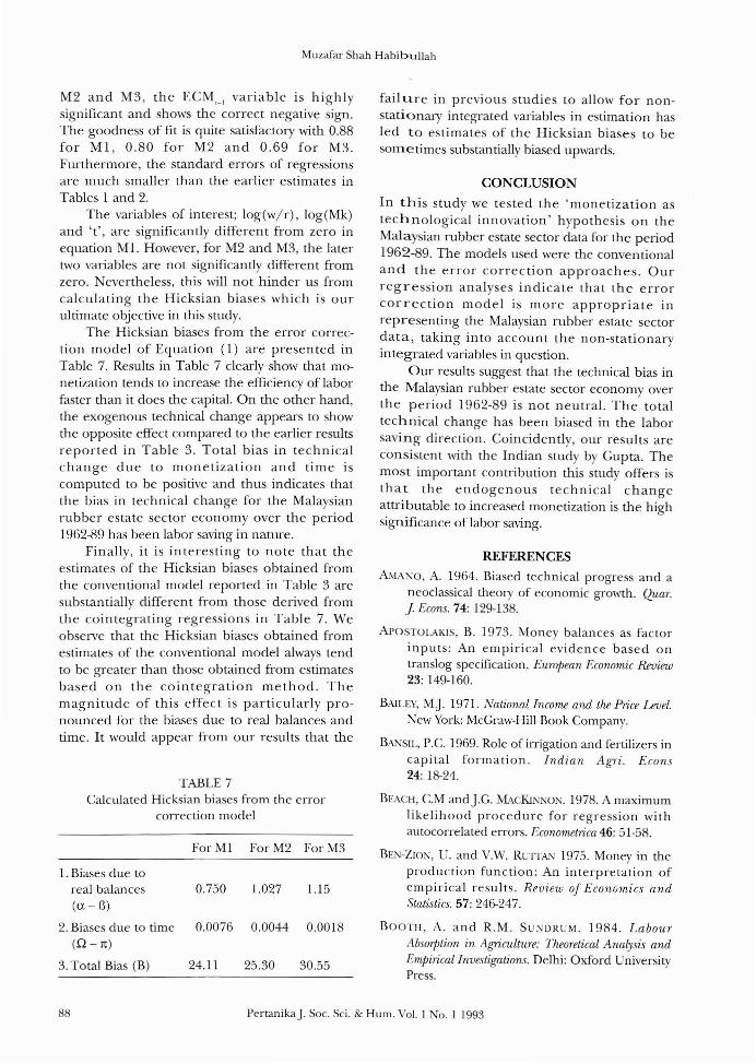
M2 and M3, the ECM,_, variable is highlysignificant and shows the correct negative sign.The goodness of fit is quite satisfactory with 0.88for Ml, 0.80 for M2 and 0.69 for M3.Furthermore, the standard errors of regressionsare much smaller than the earlier estimates inTables I and 2.

The variables of interest; log(w/r), 10g(Mk)and 't', are significantly different from zero inequation Ml. However, for M2 and M3, the latertwo variables are not significantly different fromzero. evertheless, this will not hinder us fromcalculating the Hicksian biases which is ourultimate objective in this study.

The Hicksian biases from the error correc­tion model of Equation (l) are presented inTable 7. Results in Table 7 clearly show that mo­netization tends to increase the efficiency of laborfaster than it does the capital. On the other hand,the exogenous technical change appears to showthe opposite effect compared to the earlier resultsreported in Table 3. Total bias in technicalchange due to monetization and time iscomputed to be positive and thus indicates thatthe bias in technical change for the Malaysianrubber estate sector economy over the period1962-89 has been labor saving in nature.

Finally, it is interesting to note that theestimates of the Hicksian biases obtained fromthe conventional model reported in Table 3 aresubstantially different from those derived fromthe cointegrating regressions in Table 7. Weobserve that the Hicksian biases obtained fromestimates of the conventional model always tendto be greater than those obtained from estimatesbased on the cointegration method. Themagnitude of this effect is particularly pro­nounced for the biases due to real balances andtime. It would appear from our results that the

TABLE 7Calculated Hicksian biases from the error

correction model

For MI For M2 For M3

1. Biases due toreal balances 0.750 1.027 1.15(a - 13)

2. Biases due to time 0.0076 0.0044 0.0018(Q - n)

3. Total Bias (B) 24.11 25.30 30.55

fail Ure in previous studies to allow for non­stationary integrated variables in estimation hasled to estimates of the Hicksian biases to besometimes substantially biased upwards.

CONCLUSION

In this study we tested the 'monetization astechnological innovation' hypothesis on theMalaysian rubber estate sector data for the period1962-89. The models used were the conventionaland the error correction approaches. Ourregression analyses indicate that the errorcorrection model is more appropriate inrepresenting the Malaysian rubber estate sectordata, taking into account the non-stationaryintegrated variables in question.

Our results suggest that the technical bias inthe Malaysian rubber estate sector economy overthe period 1962-89 is not neutral. The totaltechnical change has been biased in the laborsaving direction. Coincidently, our results areconsistent with the Indian study by Gupta. Themost important contribution this study offers isthat the endogenous technical changeattributable to increased monetization is the highsignificance of labor saving.

REFERENCES

AMANO, A. 1964. Biased technical progress and aneoclassical theory of economic growth. Quar.J Econs. 74: 129-138.

ArOSTOLAKIS, B. 1973. Money balances as factorinputs: An empirical evidence based ontranslog specification. European Economic Review23: 149-160.

BAll.EY, MJ. 1971. National Income and the Price Level.New York: McGraw-Hill Book Company.

BANSI!., P.C. 1969. Role of irrigation and fertilizers incapital formation. Indian Agri. Econs24: 18-24.

BEACH, C.M and J.G. MAcKiNNON. 1978. A maximumlikelihood procedure for regression withautocorrelated errors. Econometrica 46: 51-58.

BEN-ZION, U. and V.W. RUTTAN 1975. Money in theproduction function: An interpretation ofempirical results. Review of Economics andStatistics. 57: 24&-247.

BOOTH, A. and R.M. SUNDRUM. 1984. LabourAbsorption in A~iculture: Theoretical Analysis andEmpirical Investigations. Delhi: Oxford UniversityPress.

88 PertanikaJ. Soc. Sci. & HUIll. Vol. 1 0.11993

Money and Biased Technical Progress

BoYES, WJ. and D.C. KAVANAUGH. 1979. Money andproduction function: A test of specificationbias. Review oj Economics and Statistics61: 442-446.

CHOW, G.c. 1966. On the long-run and short-rundemand for money. Joumal oj Political Economy2: 111-131.

DANDRAKIS, E and E. PHELPS. 1966. A model ofinduced innovation, growth and distribution.EconomicJoumal. 76: 823-840.

DAVID, P. and TH. VAN DE KUNDERT. 1965. Biasedefficiency growth and capital-labor substitutionin the United States, 1899-1960. AmericanEconomic Review. 55: 356-394.

DESAI, B.M. 1969. Level and pattern of investment inagriculture: A micro cross-section analysis of aprogressive and a backward area in CentralGujarat. Indian]. Agric. Econs. 24: 70-79.

DICKEY, D.A. and W.A. FULLER. 1979. Distribution ofestimates for autoregressive time series withun i t root. Journal oj A merican StatisticianAssociation. 74: 427-443.

ENGLE, R.F. and C.W.]. GRANGER. 1987.Cointegration and error correction:representations, estimation and testing.Econometrica. 55: 251-276.

ENGLE, R.F. and B.S. Yoo 1987. Forecasting andtesting in coin tegrated systems. Journal ojEconometrics. 35: 143-159.

FISCHER, S. 1974. Money and the productionfunction. Economic Inquiry 12(4): 517-533.

FRIEDMAN, M. 1959. The demand for money: sometheoretical and empirical results. Journal ojPolitical Economy. 67: 327-351.

___. 1969. The Optimum Quantity oj Money andOther Essays. Chicago: Aldine PublishingCompany.

FULLER, W.A. 1976. Introduction to Statistical TimeSeries. New York: Wiley.

GHOSH, M.G. 1969. Investment behavior oftraditional and modern farms - A comparativestudy. Indian]. ojAgric. Econs. 24: 80-89.

GRANGER, C.WJ. and P. NEVVBOLD. 1977. ForecastingEconomic Time Series. New York. Academic Press.

GUPTA, K.L. 1985. Money and the bias of technicalprogress. Applied Economics. 17(1): 87-93.

HABIBULLAH, MUZAFAR SHAH. 1992. Learning by­doing in production function: the case of

Malaysian rubber estate sector. Journal ojNatural Rubber Research 7(2): 142-151.

__________ . 1989a. Determ inan ts of capi talformation in the Malaysian rubber estatesector. Journal oj Natural Rubber Research 4(4):223-232.

_____. 1989b. Technological progress andYES production function in Malaysian rubberestate sector: An empirical note. Malaysian]. ojEcon. Studies. 26(2): 43-48.

__________ . 1988. Real money balances in theproduction function of a developing economy:A preliminary study of the Malaysianagricultural sector. Pertanika. 11(3): 451-460.

HALL, S.G. 1986. An application of the Granger &Engle two-step estimation procedure to UnitedKingdom aggregate wage data. OxJord Bulletin ojEconomics and Statistics. 483: 229-239.

JOHNSON, H.G. 1969. Inside money, outside money,income, wealth and welfare in monetary theory.Journal oj Money, Credit and Banking.1: 30-45.

KHAN, A.H. and A. AHMAD. 1985. Real moneybalances in the production function of adeveloping country. Review oj Economics andStatistics. 67: 336-340.

KHAN, M.S. and P.j.K. KOURI. 1975. Real moneybalances as a factor of production: A comment.Review oj Economics and Statistics.57: 244-246

KUMAR, B. 1969. Capital formation in Indianagriculture. Indian]. ojAgric. Econs. 24: 13-17.

KURIAN, A.P. 1969. Estimates of private capitalexpenditure in agriculture during the period1966-70 to 1973-74. Indian.J. oj Agric. Econs.24: 67-70.

LEVHARI, D. and D. PATINKIN. 1968. The role ofmoney in a simple growth model. AmericanEconomic Review. 58: 713-754.

Malaysia, Bank Negara Malaysia. Quarterly EconomicBulletin, various issues.

___, Department of Statistics. Rubber StatisticsHandbook, various issues.

MORONEY,j.R. 1972. The current state of money andproduction theory. American Economic Review 62:335-343.

NADIRI, M.l. 1969. The determinants of real cashbalances in the U.S. total manufacturing sector.Quar]. Econs 83: 173-196.

Pertanika.J. Soc. Sci. & Hum. Vol. 1 No.1 1993 89

Muzafar Shah Habibullah

NICCOI.l, A. 1975. Real money balances: An omittedvariable from the production function? Acomment. Review of Economics and Statistics.57: 241-243.

IURKSE, R. 1952. Problems of Capital Formation inUnder-developed Count.,.ies. Oxford: BasilBlackwell.

PANIKAR, P.G.K. 1969. Capital formation in Indianagriculture. Indian]. ofAgric. Econs 24: 31-44.

PINDYCK, R.S. and D.L. RUBINFELD. 1981. EconometricModels and Economic Forecasts. Singapore:McGraw-Hill International Book Company.

PRAIS, Z. 1975a. Real money balances as variable inthe production function. Review of Economicsand Statistics 57: 243-244.

____. 1975b. Real money balances as variable inthe production function. Joumal ofMoney, Creditand Banking 7(4): 535-540.

RA.lAGOPAI.AN, V. and S. KRISHNAMOORTHY. 1969.Saving elasticities and strategy for capitalformation - A Micro Analysis. Indian]. of Ag7ic.

Econs. 24: 110-116.

SARWAR, G., N.S. DHAJ.JWAI. and J.F. YANAGIDA. 1989.Uncertainty and the stability of money demandfunctions for the U.S. agricultural sector. Can.]. ofAgric. Econs. 37: 279-289.

SHORT, E.D. 1979. A new look at real moneybalances as a variable in the production

function. Journal of Money, Credit and Banking11(3): 326-339.

SIMOS, E.O. 1981. Real money balances as aproductive input. Joumal of Monetmy Economics.7: 207-225.

SINAI, A. and H.H. STOKES. 1972. Real moneybalances: an omitted variable from theproduction Function? Review of Economics andStatistics. 54: 290-296.

SINGH, B. 1969. Human capital in agriculture inHaryana agriculture. Indian]. ofAg7ic. Econs. 24:106-110.

SISODIA, J.S. 1969. Capital formation in agriculturein Madhya Pradesh. Indian.J. of Agric. Econs.24: 50-59.

SUBRAHMANYAM, G.1980. Real money balances as afactor of production: some new evidence.Review ofEconomics and Statistics. 62: 280-285.

____. and T.F. COSIMANO. 1979. Money andBiased Technical Progress. Jou'mal of MonetaryEconomics 5: 497-504.

You, J.S. 1981. Monn. tech1lology and theproduction functio1l: an empirical study. Can].Econs. 14(3): 515-5~4

(Received 26 October 1991)

90 PertanikaJ. Soc. Sci. & Hum. Vol. 1 No.1 1993