Money, Banking, and Monetary Policy�

Ping HeUniversity of Illinois at Chicago

Lixin HuangCity University of Hong Kong

Randall WrightUniversity of Pennsylvania

September 15, 2006

Abstract

One important function of banks is to issue liabilities, like demanddeposits, that are relatively safe and also liquid (usable as means ofpayment). We introduce risk of theft and a safe-keeping role for banksinto monetary theory. This provides a general equilibrium frameworkfor analyzing banking in historical and contemporary contexts. Themodel can generate concurrent circulation of cash and bank liabilitiesas media of exchange (inside and outside money), and yields novel pol-icy implications. For example, negative nominal interest rates are fea-sible, and for some parameters optimal; for other parameters, strictlypositive rates (in�ation above the Friedman Rule) are optimal.

�We thank many participants in seminars and conferences for input, as well as the NSFand the Ferderal Reserve Bank of Cleveland for research support. The usual disclaimerapplies.

1

Genuine banks are distinguished from other kinds of �nancialintermediaries by the readily transferable or �spendable�natureof their IOUs, which allows those IOUs to serve as a meansof exchange, that is, money. ... Commercial bank money todayconsists mainly of deposit balances that can be transferred eitherby means of paper orders known as checks or electronically usingplastic �debit�cards. George Selgin , Banking.

1 Introduction

Banks perform many functions in modern economies, but one very important

function is to issue liabilities, like demand deposits, that are relatively safe

and also relatively liquid. Putting money in the bank obviously reduces the

risk that it will get lost or stolen without necessarily hindering too much

its use as a means of payment. Moreover, using something other than cash

reduces other risks, since one may be able to �stop payment�with a check

or credit card, e.g., if a purchase turns out to be �awed or fraudulent. While

these points may be obvious, this does not mean they are uninteresting or

unimportant for our understanding of money and banking. Yet they have

been all but ignored in the literature.1

1See Gorton and Winton (2003) for a survey of mainstream banking theory. Thisliterature has nothing to say about the medium of exchange function of money, let alonethe relation between cash and bank liabilities in performing this function. Monetarytheory along the lines of Kiyotaki and Wright (1989) is all about determining media ofexchange endogenously, but typically has nothing that resembles banks. The few papersthat do try to integrate banking and modern monetary theory include Cavalcanti andWallace (1999a, b), Cavalcanti, Erosa and Temzilides (1999, 2005), Andolfatto and Nosal(2003), Wallace (2005), Berentsen, Camera and Waller (2005), Li (2006) and Chiu andMeh (2006); some other papers in an slightly older tradition of monetary theory are citedin He, Huang and Wright (2005). None of this work discusses safekeeping. The only workthat does speak to the issue is Kahn, McAndrews and Roberds (2005), and Kahn andRoberds (2005), but they use a very di¤erent framework, and take the opposite point ofview: they assume the use of cash reduces risk since it minimizes exposure to dangers suchas �indentity theft.�While this is a �ne point, we think most people would agree thatwalking around with large quantities of cash is risky �or at least they should agree it isworth considering this case.

2

In a previous attempt to rectify this state of a¤airs (He, Huang and

Wright 2005), we introduced a risk of theft into a microfounded model of

monetary exchange based on search theory. This allowed us to study the role

of banks as institutions that provide safekeeping plus liquidity in a setting

where there is an endogenous role for a means of payment in the �rst place.

A signi�cant drawback with that analysis, however, is that we started with

a rather crude model of monetary exchange. As in all simple �rst-generation

search models (e.g. Kiyotaki and Wright 1993) we adopted the assumption

that money is indivisible and agents can only hold at most 1 unit. While

one may �nd this unsatisfying for a number of reasons, perhaps the main

limitation is that it is impossible to discuss many interesting aspects of

monetary policy, especially the e¤ect of the in�ation or nominal interest rates

on banking and on the interaction between currency and bank liabilities as

means of payment.

The goal of this paper is to bring the integration of banking and mon-

etary theory into the 21st century by reconsidering these basic ideas in the

recent generation of search models. This allows us to discuss issues and

derive results going well beyond anything in the earlier work, and provides

a genuine general equilibrium framework in which to formalize venerable

ideas about how modern banks came to be in the �rst place. Although we

do not want to dwell on history too much (see the previous paper for a few

more details), it may be helpful to review the story about safekeeping and

early banking. As told in general reference books, �The direct ancestors

of modern banks were ... the goldsmiths. At �rst the goldsmiths accepted

deposits merely for safe keeping ; but early in the 17th century their deposit

receipts were circulating in place of money and so became the �rst English

3

bank notes.�(Encyclopedia Britannica 1954, vol. 3, p. 41, emphasis added).

More specialized sources echo this view. �By the restoration of Charles

II in 1660, London�s goldsmiths had emerged as a network of bankers ...

Some were little more than pawn-brokers while others were full service

bankers. The story of their system, however, builds on the �nancial ser-

vices goldsmiths o¤ered as fractional reserve, note-issuing bankers. In the

17th century, notes, orders, and bills (collectively called demandable debt)

acted as media of exchange that spared the costs of moving, protecting and

assaying specie.� (Quinn 1997, p. 411-12, emphasis added). �The crucial

innovations in English banking history seem to have been mainly the work

of the goldsmith bankers in the middle decades of the seventeenth century.

They accepted deposits both on current and time accounts from merchants

and landowners; they made loans and discounted bills; above all they learnt

to issue promissory notes and made their deposits transferrable by �drawn

note�or cheque.�(Joslin 1954, p. 168, emphasis added).2

While to us this history is fascinating, there are also contemporary is-

sues for which our analysis is relevant. A body of work surveyed by Boyd

and Champ (2003) e.g. discusses many empirical �ndings concerning the

relation between in�ation (or interest) rates and �nancial markets, includ-

2Safekeeping was also crucial for earlier episodes in banking history, going back tothose some consider history�s �rst bankers, the Templars (Weatherford 1997; Sanello 2003).However, the goldsmiths seem to be the �rst banks whose liabilities circulated as media ofexchange. Previously, payments typically involved transferring funds from one account toanother and �generally required the presence at the bank of both payer and payee�(Kohn1999). Moreover, �In order that bank credit may be used as a means of payment, it isclearly quite essential that some convenient procedure should be instituted for assigning abanker�s debt from one creditor to another. In the infancy of deposit banking in mediaevalVenice, when a depositor wanted to transfer a sum to someone else, both had to attendthe bank in person. In modern times the legal doctrine of negotiable instruments has beendeveloped ... The document may take either of two forms: (1) a cheque, or the creditor�sorder to the bank to pay; (2) a note or the banker�s promise to pay.� (EncyclopediaBritannica 1941, vol. 3, p. 44).

4

ing the banking sector.3 While we do not attempt to address any of these

observations directly here, we think the framework provides a step in the

right direction: if one is ever to make sense of empirical results on the rela-

tion between in�ation, or interest rates, and banking, or �nancial markets

more generally, it might be useful to have a theory that tried to integrate

these markets into monetary economics more carefully. This is arguably

true because it is by now well known that taking microfoundations seriously

can make a big di¤erence in monetary economics for both qualitative and

quantitative results (see e.g. Lagos and Wright 2005).

The rest of the paper can be summarized as follows. In Section 2 we

present basic assumptions. In Section 3 we study the case with exogenous

risk of theft and no banks, and show how the value of money depends on this

risk. We show that it is possible in equilibrium to have negative nominal

interest rates, although there is a lower bound. In fact, in this model it

is optimal to go to the lower bound, which means de�ation in excess of

the Friedman Rule, i = 0. In Section 4 we endogenize the risk associated

with cash, still with no banks. In this version of the model, depending on

parameters, it may or may not be possible to have negative nominal rates,

but it will never be optimal: the optimal interest rate is either i = 0 or

i > 0. The reason that some in�ation in excess of the Friedman Rule may

be optimal is that in equilibrium it reduces the risk associated with cash.

3Here are some examples of what we have in mind. Very low nominal interest andin�ation rates are associated with low levels of investment and growth, but permanentlyhigher rates above certain threshold also adversely a¤ect growth. One interpretation isthat high in�ation leads to a low supply of funds and more credit rationing, and alsoreduces the incentive of �rms to accumulate internal funds, causing them to rely more onexternal �nancing, and increasing informational frictions in �nancial market. In�ation isalso negatively correlated with the ratio of bank assets or liquid liability to GDP when itis below 15%, but for in�ation is above 15%, the relationship disappears although thereis a �xed drop in banking development indicators.

5

In Section 5 we introduce banks when risk is exogenous. We show that

generically agents either put all or none of their money in the bank, so

we cannot get the concurrent circulation of multiple means of payment:

bank liabilities drive cash out of circulation (or vice versa) whenever bank

operating costs are small (big). The optimal policy is again i < 0, basically

because appreciation in the value of money helps o¤set banking costs. In

Section 6 we endogenize risk in the model with banks. Now we can easily

generate the concurrent circulation of multiple means of payment. In this

case, the optimal policy is generically either i < 0 or i > 0. This is interesting

because usually the Friedman Rule is extremely robust: i = 0 is the optimal

policy in a wide variety of monetary models and a variety of situations. In

Section 7 we brie�y discuss some additional issues and conclude.

2 Basic Assumptions

A [0; 1] continuum of agents live forever in discrete time. Borrowing from

Lagos and Wright (2005), hereafter referred to as LW, we assume that each

period has two markets: a centralized market denoted CM, and a decentral-

ized market denoted DM. The CM is a frictionless (Walrasian) market that

can be speci�ed quite generally, although for ease of presentation we assume

two goods, consumption x and labor `, and quasi-linear utility U(x) � `,

with U 0 > 0 � U 00. The DM is characterized by several frictions designed

to generate a role for media of exchange. First, there is a standard double-

coincidence problem, formalized here by assuming that agents specialize in

production and consumption, and that they meet and trade bilaterally.

In particular, when two agents i and j meet in the DM, the following is

true: i wants something j can produce but not vice versa with probability

6

�; j wants something i can produce but not vice versa with probability �;

and neither wants what the other produces with probability 1 � 2�, where

� 2 (0; 12).4 If i produces q units of his output for j, the latter gets utility

u(q) and the former su¤ers disutility c(q), where we assume u0, c0 > 0,

u00 < 0, c00 � 0, u(0) = c(0) = 0, and u(Q) = c(Q) = 0 for some Q > 0.

Denote by q� the the e¢ cient amount of production and consumption, i.e.

the solution to u0(q) = c0(q).

To generate a role for a medium of exchange we still need to have imper-

fect enforcement of credit, so that i cannot simply o¤er j an IOU in exchange

for his output, promising to pay in the next CM where he can acquire the

funds by e.g. supplying labor. The standard approach is to assume some

form of anonymity �basically, j does not know who i is, which means i could

renege on his promise without fear of repercussion. This makes some tangi-

ble medium of exchange essential, as in most modern monetary economics.5

In addition, we add another friction: the possibility that money can be

stolen in the DM. Hence, agents in the CM may choose to deposit their cash

into a bank account, which is assumed for simplicity to be perfectly safe,

and can still be used to make DM payments.

We emphasize that the assumption that agents can use the liabilities of

a bank as a means of payment does not con�ict with the assumption that

these agents are anonymous in some bilateral meetings. A seller may be

willing to accept a claim on a bank from a person he does not know, and

hence to whom he would never extend private credit, if he knows the bank.

4 It would add nothing but notation, and so we do not bother, to allow some double-coincidence meetings, where i and j both want what the other can produce.

5See Kocherlakota (1998), Wallace (2001) or Corbae et al. (2003) for formal discussionsof anonymity and the essentiality of a medium of exchange.

7

There are many examples in the real world that correspond more or less to

what we have in the model. Travellers�s Checks are a leading case; debit

cards constitute a modern incarnation. The key point is that these can be

used as means of payment almost as easily as cash �i.e. they are very liquid

�and they are extremely safe.6

Agents do their banking in the CM, and trade using either cash or bank

liabilities in the DM. However, paying with bank liabilities entails a fee �.

Banks have a resource cost a > 0 per dollar on deposit, since safekeeping

is not free. Also, they are required legally to keep a fraction � of deposits

on reserve, while the rest can be out on loan. In the benchmark model we

assume � = 1; in this case banks must keep all deposits in the vault, and

hence competition implies � = a. Let M be the aggregate stock of money

at the start of the CM, which evolves over time according to M = (1+�)M

where we use z for the value of any generic variable z next period. In steady

state, � is the in�ation rate. The government budget is �M+T = pG , where

T is a lump sum nominal tax and G is exogenous government consumption.

3 Exogenous Theft

In this section we study the model where the risk of holding money is ex-

ogenous: there is simply a �xed fraction of the population � 2 (0; 1) that are

thieves and try to rob you if you meet them in the DM. With probability

6American Express Travellers�s Checks in particular are safe for two reasons: �rst,people are less interested in stealing them (than cash) because in order to spend them onehas to match the signature of the original purchaser; and second, if they are lost stolen,American Express refunds your money. Of course, not all bank liabilities are perfectlysafe �bank notes e.g. were historically about as easy to steal as coins. And bank failuresor bank robberies do occur. It seems obvious, however, that carrying a Travellers�Check,a certi�ed check, a bank card with a PIN number, etc. is typically less risky than carryinga bundle of currency.

8

2 (0; 1) they succeed, and with probability 1� they fail and walk away

empty handed. Thieves do not produce or consume anything in the DM,

but act just like honest agents in the CM. We �rst study the case where

the only asset is money �i.e. for now there are no banks. Let Wj(m) and

Vj(m) be the value functions for type j entering the CM and the DM with

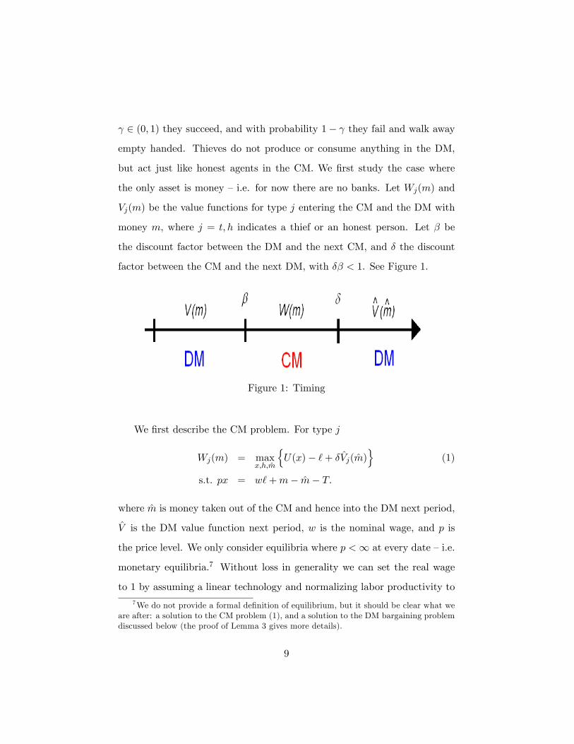
money m, where j = t; h indicates a thief or an honest person. Let � be

the discount factor between the DM and the next CM, and � the discount

factor between the CM and the next DM, with �� < 1. See Figure 1.

Figure 1: Timing

We �rst describe the CM problem. For type j

Wj(m) = maxx;h;m

nU(x)� `+ �Vj(m)

o(1)

s.t. px = w`+m� m� T:

where m is money taken out of the CM and hence into the DM next period,

V is the DM value function next period, w is the nominal wage, and p is

the price level. We only consider equilibria where p <1 at every date �i.e.

monetary equilibria.7 Without loss in generality we can set the real wage

to 1 by assuming a linear technology and normalizing labor productivity to7We do not provide a formal de�nition of equilibrium, but it should be clear what we

are after: a solution to the CM problem (1), and a solution to the DM bargaining problemdiscussed below (the proof of Lemma 3 gives more details).

9

unity, so w = p; it is easy to allow a concave technology but this adds little

except notation for the current application.

A thief has no reason to bring money into the DM. Hence the solution to

his problem is mt = 0, xt = x� where U 0(x�) = 1, and `t = x��m=p+ T=p.

For an honest person, who may choose to bring money into the DM in order

to consume, the solution to his problem satis�es �V 0h(mh) = 1=p, xh = x�

and `h = x��(m� m) =p+T .8 Notice that m does not depend on m; hence

every honest person chooses the same mh = �m, where �m �M=(1� �). The

result that all agents of the same type choose the same m, regardless of their

history, follows from quasi-linear CM utility, and is what keeps the analysis

tractable. Another convenient feature is that the CM value functions are

linear: W 0h(m) =W

0t(m) = 1=p 8m.

Consider now the DM. For a thief, who in equilibrium carries no money

into this market,

Vt(0) = ��Wt(0) + (1� �) [ �Wt( �m) + (1� )�Wt(0)] : (2)

The �rst term is his payo¤ to meeting another thief, which occurs with

probability �, and implies he goes to the next CM empty handed. The

second term is his payo¤ to meeting an honest person, which occurs with

probability 1 � �, in which case with probability he is successful and

goes to the CM with �m, while with probability 1 � he is not successful

and goes to the CM empty handed. Since Wt is linear, we have Vt(0) =

�Wt(0) + (1� �) � �m=p, which will come in handy later.

8These results assume interior solutions for `, which we can guarantee as in LW withsuitable restrictions on preferences. They also assume the second order condition holdsfor m; we check below that this is true in any equilibrium.

10

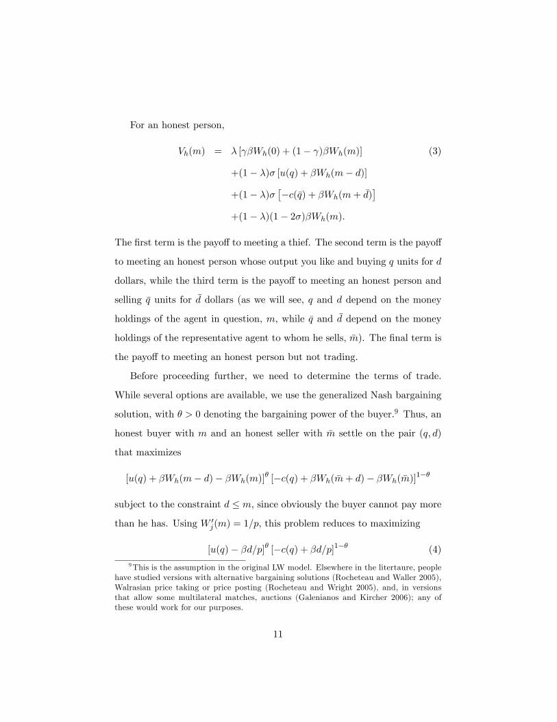
For an honest person,

Vh(m) = � [ �Wh(0) + (1� )�Wh(m)] (3)

+(1� �)� [u(q) + �Wh(m� d)]

+(1� �)���c(�q) + �Wh(m+ �d)

�+(1� �)(1� 2�)�Wh(m):

The �rst term is the payo¤ to meeting a thief. The second term is the payo¤

to meeting an honest person whose output you like and buying q units for d

dollars, while the third term is the payo¤ to meeting an honest person and

selling �q units for �d dollars (as we will see, q and d depend on the money

holdings of the agent in question, m, while �q and �d depend on the money

holdings of the representative agent to whom he sells, �m). The �nal term is

the payo¤ to meeting an honest person but not trading.

Before proceeding further, we need to determine the terms of trade.

While several options are available, we use the generalized Nash bargaining

solution, with � > 0 denoting the bargaining power of the buyer.9 Thus, an

honest buyer with m and an honest seller with �m settle on the pair (q; d)

that maximizes

[u(q) + �Wh(m� d)� �Wh(m)]� [�c(q) + �Wh( �m+ d)� �Wh( �m)]

1��

subject to the constraint d � m, since obviously the buyer cannot pay more

than he has. Using W 0j(m) = 1=p, this problem reduces to maximizing

[u(q)� �d=p]� [�c(q) + �d=p]1�� (4)9This is the assumption in the original LW model. Elsewhere in the litertaure, people

have studied versions with alternative bargaining solutions (Rocheteau and Waller 2005),Walrasian price taking or price posting (Rocheteau and Wright 2005), and, in versionsthat allow some multilateral matches, auctions (Galenianos and Kircher 2006); any ofthese would work for our purposes.

11

subject to d � m. This immediately implies that the solution does not

depend on �m and depends on m i¤ the constraint binds.

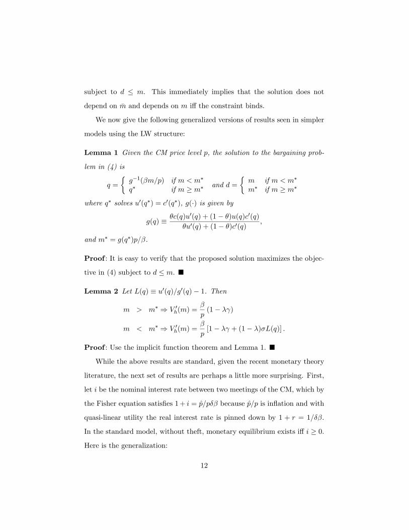
We now give the following generalized versions of results seen in simpler

models using the LW structure:

Lemma 1 Given the CM price level p, the solution to the bargaining prob-

lem in (4) is

q =

�g�1(�m=p) if m < m�

q� if m � m� and d =�m if m < m�

m� if m � m�

where q� solves u0(q�) = c0(q�), g(�) is given by

g(q) � �c(q)u0(q) + (1� �)u(q)c0(q)�u0(q) + (1� �)c0(q) ;

and m� = g(q�)p=�.

Proof : It is easy to verify that the proposed solution maximizes the objec-

tive in (4) subject to d � m. �

Lemma 2 Let L(q) � u0(q)=g0(q)� 1. Then

m > m� ) V 0h(m) =�

p(1� � )

m < m� ) V 0h(m) =�

p[1� � + (1� �)�L(q)] :

Proof : Use the implicit function theorem and Lemma 1. �

While the above results are standard, given the recent monetary theory

literature, the next set of results are perhaps a little more surprising. First,

let i be the nominal interest rate between two meetings of the CM, which by

the Fisher equation satis�es 1+ i = p=p�� because p=p is in�ation and with

quasi-linear utility the real interest rate is pinned down by 1 + r = 1=��.

In the standard model, without theft, monetary equilibrium exists i¤ i � 0.

Here is the generalization:

12

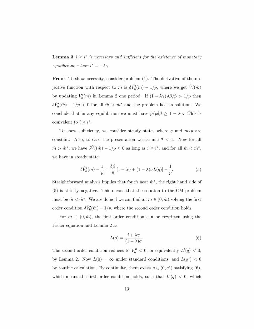
Lemma 3 i � i� is necessary and su¢ cient for the existence of monetary

equilibrium, where i� � �� .

Proof : To show necessity, consider problem (1). The derivative of the ob-

jective function with respect to m is �V 0h(m) � 1=p, where we get V 0h(m)

by updating V 0h(m) in Lemma 2 one period. If (1� � ) ��=p > 1=p then

�V 0h(m) � 1=p > 0 for all m > m� and the problem has no solution. We

conclude that in any equilibrium we must have p=p�� � 1 � � . This is

equivalent to i � i�.

To show su¢ ciency, we consider steady states where q and m=p are

constant. Also, to ease the presentation we assume � < 1. Now for all

m > m�, we have �V 0h(m) � 1=p � 0 as long as i � i�; and for all m < m�,

we have in steady state

�V 0h(m)�1

p=��

p[1� � + (1� �)�L(q)]� 1

p: (5)

Straightforward analysis implies that for m near m�, the right hand side of

(5) is strictly negative. This means that the solution to the CM problem

must be m < m�. We are done if we can �nd an m 2 (0; m) solving the �rst

order condition �V 0h(m)� 1=p, where the second order condition holds.

For m 2 (0; m), the �rst order condition can be rewritten using the

Fisher equation and Lemma 2 as

L(q) =i+ �

(1� �)� : (6)

The second order condition reduces to V 00h < 0, or equivalently L0(q) < 0,

by Lemma 2. Now L(0) = 1 under standard conditions, and L(q�) < 0

by routine calculation. By continuity, there exists q 2 (0; q�) satisfying (6),

which means the �rst order condition holds, such that L0(q) < 0, which

13

means the second order condition holds. Once we have q, Lemma 1 gives

m = pg(q)=�, where m < m� since q < q�(Lemma 1). Then p = � �m=g(q) is

determined to clear the market with �m =M=(1��). The other CM variables

(xj ; `j) are determined as discussed above. This completes construction of

a steady state equilibrium. �

In the proof of Lemma 3 we assumed � < 1, but the case � = 1 is not

much harder.10 More substantively, L(q) de�ned in Lemma 2 represents

a liquidity premium on cash, which (6) sets equal to the holding cost per

period: the nominal rate i plus risk factor � , times the expected number

of periods until one spends the money, 1=(1 � �)�. Notice in fact that (6)

must hold in any equilibrium, and not just any steady state, since it follows

simply from the problem of choosing m in the CM. Because L0(q) < 0, q

increases as we lower i towards i�. One can also show q is increasing in �.

We know that q � q�, with strict inequality except when � = 1 and i = i�,

and hence we maximize expected utility by raising q as high as possible,

which means i = i�. At i� we have q = q, where L(q) = 0, and q � q� with

strict equality i¤ � = 1. Hence, we do not get the �rst best q� at the optimal

i� unless buyers have all the bargaining power.

Proposition 1 With exogenous theft and no banks, there exists a monetary

equilibrium i¤ i � i� = �� . In equilibrium @q=@i < 0, the optimal policy

is i = i�, and it implies q = q, where q � q� with strict equality i¤ � = 1.

Proof : Follows directly from the discussion in the text. �10The only di¢ culty when � = 1 is that while the limit as m % m� of (5) is still

negative it is only strictly negative when i > i�. If � = 1 and i = i� the CM problem issolved at m = m�, but also at any m > m� since (5) is 0 for all m � m�. This nuisanceindeterminacy can be eliminated if we assume i > i� and consider only the limit as i& i�

(i.e. we only consider equilibria at i = i� that are the limit of equilibria as i& i�).

14

The fact that nominal rates can be negative is unusual in monetary

theory, but not so surprising given that cash is risky. The usual arbitrage

argument to rule it out is that one could borrow a dollar today, pay back

1 + i tomorrow, and have money left over if i < 0. But now the dollar

might get stolen! Arbitrage here says only that nominal rates cannot be

too negative: i � �� . The exact expression depends on speci�c modeling

assumptions, but the bigger point is that one has to take into account the

probability that any arbitrage attempt will go wrong. Empirically, i < 0 is

not uncommon �an obvious example is American Express Travelers�Checks,

but any demand deposit with a zero or low nominal interest rate and positive

fees (e.g. a charge per check) e¤ectively pays i < 0.

4 Endogenous Theft

We now endogenize the decision to be a thief, and hence the risk of using

cash. Now, we cannot have � = 1 in any monetary equilibrium, since no

one will work to acquire cash when all that happens is that it gets stolen.

Therefore we look for equilibria with � 2 [0; 1). To this end, let �(m) =

Wh(m) � Wt(m), and note that � actually does not depend on m, since

both Wh and Wt are linear with slope 1=p. Then an equilibrium requires,

in addition to the conditions discussed in Section 3,

� = 0 if � > 0 and � = 0 if � 2 (0; 1): (7)

Given what we learned in the previous section, we can write the equilib-

rium payo¤s in the DM as

Vt(0) = �Wt(0) + �(1� �) m

p

Vh(m) = �Wh(0) + (1� �)� [u(q)� c(q)] + � (1� � )m

p:

15

Similarly, in the CM,

Wt(m) = U(x�)� x� � Tp+m

p+ �Vt(0)

Wh(m) = U(x�)� x� � Tp+m

p+ �Vh(m)�

m

p:

Updating Vt and Vh one period, inserting these into Wt and Wh, and impos-

ing in steady state, we have

(1� ��)Wt(0) = U(x�)� x� � Tp+ ��(1� �) m

p

(1� ��)Wh(0) = U(x�)� x� � Tp+ �(1� �)� [u(q)� c(q)]

+��(1� � )mp� mp

Using these, as well as the bargaining solution �m=p = g(q) and the

Fisher equation, we can simplify � to arrive at

� ' (1� �)� [u(q)� c(q)]� (i+ )g(q); (8)

where the notation A ' B means A and B have the same sign. There are

two possible types of equilibria. One possibility is � 2 (0; 1), which requires

� = 0, and therefore

� = 1� (i+ )g(q)

� [u(q)� c(q)] : (9)

The other possibility is � = 0, which requires � � 0. In either case we still

have to satisfy equilibrium condition (6) for q from Section 3.

To �x ideas, consider an example with � = 1, which means g(q) = c(q),

and functional forms u(q) = q� and c(q) = q (general results follow below).

Consider �rst equilibria with � > 0. Then (9) and (6) imply:

� =� � (1� �)(� + i) � �(1� �) (10)

q =

��(1� �)

� 11��

(11)

16

The solution to (11) q = ~q is independent of i. Also, � > 0 i¤ i < i0 �

� =(1��)��, and � < 1 i¤ i > � which is not binding since i � i� = ��

(Lemma 3 applies here). Hence, equilibrium with � 2 (0; 1) exists i¤ i < i0.

Now consider equilibria with � = 0, which means

q =

���

� + i

� 11��

: (12)

An equilibrium with � = 0 requires � � 0, which holds i¤ i � i0. Note that

q = qi is decreasing in i in this equilibrium.

Summarizing, we have two generic cases.

Case (i) � (1� �) > � . Then i0 < 0, and equilibrium exists i¤ i � i� = 0.

In this equilibrium � = 0, and (12) gives q = qi as a decreasing function of

i. Given � = 1, in this example, we get qi = q� = �1=(1��) at i = 0; more

generally we get qi = q at i = 0.

Case (ii) � (1� �) < � . Then i0 > 0. An equilibrium with � = 0 and

q = qi given by (12) exists i¤ i � i0, and an equilibrium with � > 0 and

q = ~q given by (11) exists i¤ i 2 (i�; i0). Now i� = � � is endogenous, but

it is easy to check that � % 1 as i & i�, and hence i� = � . Since ~q is

independent of i when � > 0, (10) implies that � is linearly decreasing in i

in this equilibrium.

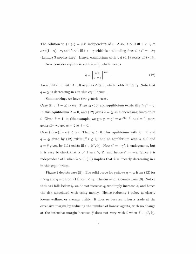
Figure 2 depicts case (ii). The solid curve for q shows q = qi from (12) for

i > i0 and q = ~q from (11) for i < i0. The curve for � comes from (9). Notice

that as i falls below i0 we do not increase q, we simply increase �, and hence

the risk associated with using money. Hence reducing i below i0 clearly

lowers welfare, or average utility. It does so because it hurts trade at the

extensive margin by reducing the number of honest agents, with no change

at the intensive margin because ~q does not vary with i when i 2 [i�; i0].

17

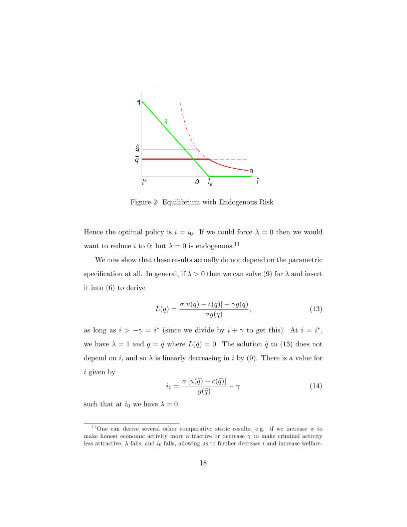
Figure 2: Equilibrium with Endogenous Risk

Hence the optimal policy is i = i0. If we could force � = 0 then we would

want to reduce i to 0; but � = 0 is endogenous.11

We now show that these results actually do not depend on the parametric

speci�cation at all. In general, if � > 0 then we can solve (9) for � and insert

it into (6) to derive

L(q) =�[u(q)� c(q)]� g(q)

�g(q); (13)

as long as i > � = i� (since we divide by i + to get this). At i = i�,

we have � = 1 and q = q where L(q) = 0. The solution ~q to (13) does not

depend on i, and so � is linearly decreasing in i by (9). There is a value for

i given by

i0 =� [u(~q)� c(~q)]

g(~q)� (14)

such that at i0 we have � = 0.

11One can derive several other comparative static results; e.g. if we increase � tomake honest economic activity more attractive or decrease to make criminal activityless attractive, � falls, and i0 falls, allowing us to further decrease i and increase welfare.

18

We know from the example that i0 can be positive or negative. If i0 < 0

then i� = 0, equilibrium exists i¤ i � 0, and � = 0.12 And if i0 > 0, the

situation is qualitatively exactly as in Figure 2. Summarizing these �ndings:

Proposition 2 With endogenous theft and no banks, there is a value of i0,

that can be positive or negative, with the following properties. If i0 < 0 then

equilibrium exists i¤ i � 0, and it implies � = 0 and @q=@i < 0. In this case

welfare is maximized at i = 0. If i0 > 0 then equilibrium exists with � = 0

i¤ i � i0 and it implies @q=@i < 0, while equilibrium exists with � > 0 i¤

i� � i < i0 where now i� = � , and it implies q = ~q independent of i. In

this case, welfare is maximized at i = i0.

Proof : Follows directly from the discussion in the text.

Perhaps the most interesting part of these results is that welfare can be

maximized at i = i0 > 0. It is interesting because the Friedman Rule i = 0

is so robust in monetary economics. Now in the previous section we already

found it was optimal to have i = i� < 0, but this is in the same spirit as

the Friedman Rule � drive in�ation and nominal interest rates as low as

possible. Here it can be optimal to have more in�ation than the Friedman

Rule. Curiously enough, the reason that a little bit of in�ation may be good

is that it keeps people honest.

5 Banks and Exogenous Theft

It is time to allow agents in the CM to put money in the bank. The model

here is quite di¤erent from the one in He et al. (2005), which is nonconvex12More formally, suppose i0 < 0 and there is an equilibrium with i < 0. We require

i � � �, and hence � > 0. Using (9), i � � � reduces to (i+ )L(q) � 0. By de�nition,i0 = �L(q) is the value of i that makes � = 0; hence the previous inequality reduces to(i+ )i0=� � 0, which contradicts i0 < 0.

19

due to indivisible money. In that setup, some agents put money in the

bank, others do not, and equilibrium determines the fraction of each. In the

current convex model, all agents put a fraction b of their money in the bank.

For now, assume 100% required reserves, and a banking cost of a dollars per

dollar deposited. The equilibrium fee charged depositors is � = a (so that

the real cost does not depend on the absolute price level). We assume with

no loss in generality that the cost and fee are paid in the next DM. Other

than being perfectly safe, bank deposits are just like money.13

A thief�s CM problem is unchanged. His DM payo¤ is

Vt(0) = ��Wt(0) + (1� �)� �Wt( �m� �b �m) + (1� )�Wt(0)

�;

given the representative honest agent now carries (1� �b) �m in cash and has

�b �m in the bank. An honest person�s CM problem becomes

Wh(m) = maxx;m;b

�U(x)� x+ m� T � m

p+ �Vh(m; b)

�;

after substituting the budget equation, where m in this expression is money

after paying fees to the bank. The constraint in the DM is still d � m, the

bargaining solution is still given by Lemma 1, and the DM payo¤ is

Vh(m; b) = � [ �Wh (bm� bma) + (1� )�Wh (m� bma)]

+(1� �)� [u(q) + �Wh (m� d� bma)]

+(1� �)���c(�q) + �Wh

�m+ �d� bma

��+(1� �)(1� 2�)�Wh(m� bma):

13Of course, we do not need deposits to be perfectly safe, only safe relative to cash. Inprinciple, the framework could accomodate bank failures or bank robbery, or could allowagents to steal your checkbook with some probability.

20

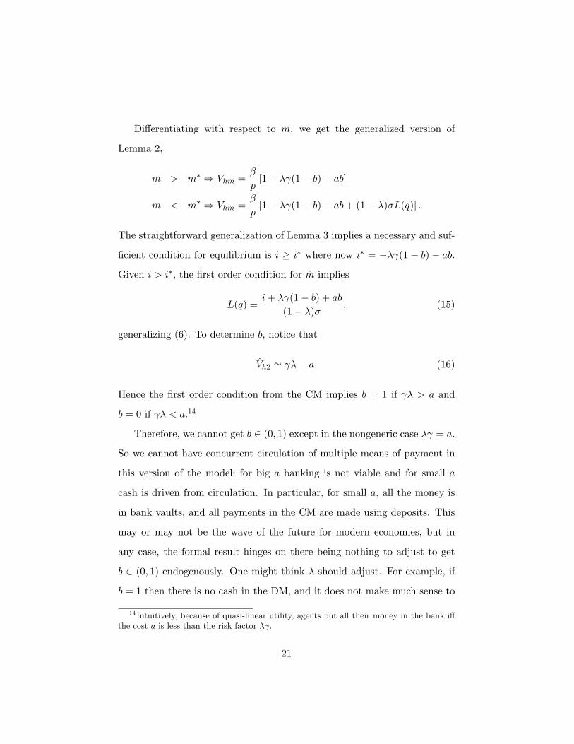
Di¤erentiating with respect to m, we get the generalized version of

Lemma 2,

m > m� ) Vhm =�

p[1� � (1� b)� ab]

m < m� ) Vhm =�

p[1� � (1� b)� ab+ (1� �)�L(q)] :

The straightforward generalization of Lemma 3 implies a necessary and suf-

�cient condition for equilibrium is i � i� where now i� = �� (1 � b) � ab.

Given i > i�, the �rst order condition for m implies

L(q) =i+ � (1� b) + ab

(1� �)� ; (15)

generalizing (6). To determine b, notice that

Vh2 ' �� a: (16)

Hence the �rst order condition from the CM implies b = 1 if � > a and

b = 0 if � < a.14

Therefore, we cannot get b 2 (0; 1) except in the nongeneric case � = a.

So we cannot have concurrent circulation of multiple means of payment in

this version of the model: for big a banking is not viable and for small a

cash is driven from circulation. In particular, for small a, all the money is

in bank vaults, and all payments in the CM are made using deposits. This

may or may not be the wave of the future for modern economies, but in

any case, the formal result hinges on there being nothing to adjust to get

b 2 (0; 1) endogenously. One might think � should adjust. For example, if

b = 1 then there is no cash in the DM, and it does not make much sense to

14 Intuitively, because of quasi-linear utility, agents put all their money in the bank i¤the cost a is less than the risk factor � .

21

be a thief. Hence, in the next section, we endogenize �. First, we summarize

the above results.

Proposition 3 With exogenous theft and banks, if � > a then b = 1,

and if � < a then b = 0. In either case, equilibrium exists i¤ i � i� =

�� (1� b)� ab, and it implies @q=@i < 0. The optimal policy is i = i�.

Proof : Follows directly from the discussion in the text.

6 Banks and Endogenous Theft

Generalizing the expressions in Section 4, we have

(1� ��)Wt(0) = U(x�)� x� � Tp+ ��(1� �) (1� b)m

p

(1� ��)Wh(0) = U(x�)� x� � Tp+ �(1� �)�[u(q)� c(q)]

+��[1� � (1� b)� ab]mp� mp;

and the analog of (8) is

� ' (1� �)� [u(q)� c(q)]� [i+ (1� b) + ab]g(q): (17)

There are three possibilities for equilibrium: b = 1, b = 0, and b 2 (0; 1).

But we cannot have b = 1 as long as a > 0: if b = 1 then no one holds cash,

which leads to � = 0, which means b = 1 cannot be a best response. Hence

we restrict attention to b 2 [0; 1).

Consider equilibrium with b = 0, which is a best response i¤ � � a,

by (16). In this case we determine q and � exactly as in Section 4. In

particular, to repeat the relevant parts of Proposition 2: � 2 (0; 1) implies

q = ~q is independent of i; � 2 (0; 1) i¤ i < i0; if i0 < 0 then i� = 0 and

22

� = 0; and if i0 > 0 then i� = � , in which case � > 0 for i 2 [i�; i0) and

� = 0 for i � i0. Given this, we check the best response condition. If � = 0

then � � a, and b = 0 is obviously a best response. The only nontrivial

case is i0 > 0 and i 2 [i�; i0), where � 2 (0; 1) is given by (9). In this case

� � a i¤ i � i1, where

i1 �( � a)�[u(~q)� c(~q)]

g(~q)� =

�1� a

�i0 � a: (18)

We conclude that when i0 > 0 and i 2 [i�; i0), b = 0 is an equilibrium i¤

i � i1.

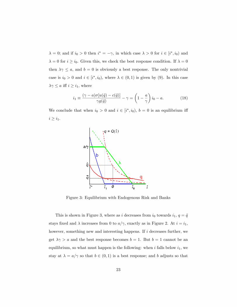
Figure 3: Equilibrium with Endogenous Risk and Banks

This is shown in Figure 3, where as i decreases from i0 towards i1, q = ~q

stays �xed and � increases from 0 to a= , exactly as in Figure 2. At i = i1,

however, something new and interesting happens. If i decreases further, we

get � > a and the best response becomes b = 1. But b = 1 cannot be an

equilibrium, so what must happen is the following: when i falls below i1, we

stay at � = a= so that b 2 (0; 1) is a best response; and b adjusts so that

23

� = a= is a best response. Hence, equilibrium for i 2 [i�; i1) is determined

by three conditions: (i) b 2 (0; 1) is a best response, which means � = a= ;

(ii) � 2 (0; 1) is a best response, which means � = 0, or

� = 1� [i+ ab+ (1� b)] g(q)� [u(q)� c(q)] ; (19)

and (iii) q satis�es the usual condition (15).

The interesting new outcome here is b 2 (0; 1), where banks operate

and DM transactions use both deposits and money.15 To discuss it further,

assume a < (because 0 < b < 1 requires � = a= < 1). Since i� = �a, in

this case, (18) implies i1 2 (i�; i0). Now, given i 2 [i�; i1), this equilibrium

exists, and has a nice recursive structure: �rst set � = a= ; then (15) reduces

to

L(q) = (i+ a)

�( � a) ; (20)

which can be solved for q = qi with @qi=@i < 0; then �nally (19) can be

solved for

bi =i+

� a �� [u(qi)� c(qi)]

g(qi): (21)

Notice bi = 1�� [u(�q)� c(�q)] = g(�q) < 1 at i� and bi = 0 at i = i1, as shown

in Figure 3.

We summarize what we know as follows.16

15 In fact, each buyer makes every purchase using both, but this stands in for the ideathat agents make some purchases with one and some purchases with the other. To getthis in the model, formally, we would need to relax assumption that they make only onepurchase in each DM, or change things so that they sometimes spend less than their totalresources in the DM, say because the utility of a seller�s output is random (it depends onwho you meet), as has been done in several other applications of the basic LW framework.If one wanted to pursue this it might also be useful to add a �xed cost each time depositsare used for a payment.

16The only thing we do not know for certain about this version of the model is, inequilibrium with b 2 (0; 1), do we have @b=@i < 0? We could not prove this generally,although it was always true in examples. Consider e.g. � = 1, u(q) = q� and c(q) = q

24

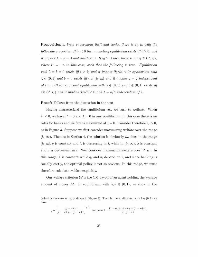
Proposition 4 With endogenous theft and banks, there is an i0 with the

following properties. If i0 < 0 then monetary equilibrium exists i¤ i � 0, and

it implies � = b = 0 and @q=@i < 0. If i0 > 0 then there is an i1 2 (i�; i0),

where i� = �a in this case, such that the following is true. Equilibrium

with � = b = 0 exists i¤ i > i0 and it implies @q=@i < 0; equilibrium with

� 2 (0; 1) and b = 0 exists i¤ i 2 (i1; i0) and it implies q = ~q independent

of i and @�=@i < 0; and equilibrium with � 2 (0; 1) and b 2 (0; 1) exists i¤

i 2 (i�; i1) and it implies @q=@i < 0 and � = a= independent of i.

Proof : Follows from the discussion in the text.

Having characterized the equilibrium set, we turn to welfare. When

i0 � 0, we have i� = 0 and � = 0 in any equilibrium; in this case there is no

roles for banks and welfare is maximized at i = 0. Consider therefore i0 > 0,

as in Figure 3. Suppose we �rst consider maximizing welfare over the range

[i1;1). Then as in Section 4, the solution is obviously i0, since in the range

[i1; i0], q is constant and � is decreasing in i, while in [i0;1), � is constant

and q is decreasing in i. Now consider maximizing welfare over [i�; i1]. In

this range, � is constant while qi and bi depend on i, and since banking is

socially costly, the optimal policy is not so obvious. In this range, we must

therefore calculate welfare explicitly.

Our welfare criterionW is the CM payo¤ of an agent holding the average

amount of money M . In equilibrium with �; b 2 (0; 1), we show in the

(which is the case actually shown in Figure 3). Then in the equilibrium with b 2 (0; 1) wehave

q =

�( � a)��

(i+ a) + ( � a)�

� 11��

and b = 1� (1� �)[(i+ a) + ( � a)�]� ( � a) :

25

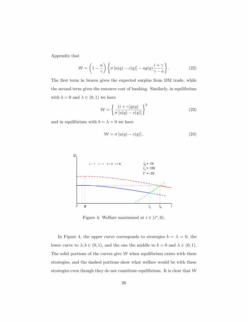
Appendix that

W =

�1� a

��� [u(q)� c(q)]� ag(q) i+

� a

�: (22)

The �rst term in braces gives the expected surplus from DM trade, while

the second term gives the resource cost of banking. Similarly, in equilibrium

with b = 0 and � 2 (0; 1) we have

W =

�(i+ )g(q)

� [u(q)� c(q)]

�2(23)

and in equilibrium with b = � = 0 we have

W = � [u(q)� c(q)] : (24)

Figure 4: Welfare maximized at i 2 (i�; 0).

In Figure 4, the upper curve corresponds to strategies b = � = 0, the

lower curve to �; b 2 (0; 1), and the one the middle to b = 0 and � 2 (0; 1).

The solid portions of the curves give W when equilibrium exists with these

strategies, and the dashed portions show what welfare would be with these

strategies even though they do not constitute equilibrium. It is clear thatW

26

is either maximized globally at i = i0, or at some point i 2 [i�; i1]. In fact,

we show in the Appendix that the maximum over the range [i�; i1] occurs

at i < 0, but it could be either i = i� or i 2 (i�; 0). In Figure 4, the global

maximum occurs at i 2 (i�; 0), but it is easy construct examples where it

occurs at i0. We summarize as follows.

Proposition 5 With endogenous theft and banks, if i0 < 0 then the optimal

policy is i = 0, and if i0 > 0 then the optimal policy may be either i 2 [i�; 0)

or i = i0 > 0.

Proof : Follows from the discussion in the text.

We think i0 > 0 is most interesting, of course, and recall from Section 4

that it is easy for this to occur in examples. In this case, we never want to

run the Friedman Rule, but either i < 0 or i > 0. Which of these is globally

optimal depends on parameters. In words, the disadvantage of i = i0 > 0 is

that q is very low, but the advantage is that it implies � = b = 0, which is

good because it eliminates both criminals and bankers! Moving outside the

con�nes of the formal analysis, the idea is that if we set in�ation too low

we may encourage undesirable behavior (in the model, crime), which is not

only unproductive, but, in general equilibrium, diverts resources to combat

such behavior (in the model, banking).

7 Conclusion

We have developed a model where there is an essential role for media of

exchange, the choice of which is endogenous. Agents may use cash but this

is relatively risky; they may use bank liabilities but this is costly; or they may

use some of each. We think this theory is interesting because it is based on

27

the actual factors underlying the historical development of modern banking,

going back at least to the goldsmiths in England. Additionally, it generates

some novel predictions concerning monetary policy. It is feasible to have

negative nominal interest rates, and for some parameter values, i < 0 is in

fact optimal. For other parameter values, it is optimal to have i > 0. It is

certainly not true that the Friedman Rule is optimal, in general, which is

certainly di¤erent from most of monetary economics.

Having a model with multiple (endogenous) means of payment seems

useful to the extent that one is interested in payments systems generally,

and especially if one is interested in empirical or policy issues such as those

mentioned in the Introduction related to the impact of in�ation on banking

and on the competition between money and other assets. Having said this,

we understand our set up is simplistic. The idea was to take a �rst cut at

modeling money and banking in a logically consistent framework; alterna-

tive environments should be considered. For example, one could replace the

brutality of theft with the subtlety of lemons problems, as in the money

models of Williamson and Wright (1994), Trejos (1997), and Berentsen and

Rocheteau (2004). Monetary policy would still impact on incentives in in-

teresting ways, but the analysis may appear more �modern� if couched in

terms of private information rather than crime.

Other extensions worth considering include reducing the reserve ratio

below � = 1 and deriving the money multiplier, as we did in the earlier

paper. It would be more complicated in this model, however, because it

is less straight forward to derive a demand for loans with divisible money;

hints as to how to proceed are contained in Berentsen et al. (2005) and

Chiu and Meh (2006). A nice thing about � < 1 is that we get � < a,

28

since banks earn revenue from loans as well as fees, and we even get � < 0

(interest on checking) when a and � are small. The problem when � < 0,

of course, is that we do not get b < 1, since bank liabilities are as liquid as

money, safer, and yield a higher return. This is �ne if one wants to capture

a �cashless economy.� But one could also add some feature to make bank

liabilities less liquid �say, some agents do not accept checks because ... We

are now getting into serious issues in monetary theory that will have to wait

for additional research.

29

Appendix

Here we verify some claims made in Section 6. First we derive the expressions

for welfare.

In equilibrium with �; b 2 (0; 1), we have Wh(M) = Wt(M), and we

compute

(1� ��)Wt(M) = (1� ��)Wt(0) + (1� ��)M

p

= U(x�)� x� + ��(1� �) (1� b)mp+ (1� ��) m(1� �)

p

= U(x�)� x� + Mp[�� (1� b) + 1� �� + �] ;

using T = ��M , M = m(1 � �), and m=p = m=p. Using m=p = g(q)=�

and the Fisher equation, this becomes

(1� ��)Wt(M) = U(x�)� x� + �(1� �)g(q) [i+ (1� b)] :

After inserting � = a= , eliminating b using (21), and performing routine

simpli�cations, we arrive at

(1� ��)Wt(M) = U(x�)�x�+ �

�1� a

��� [u(q)� c(q)]� ag(q) i+

� a

�:

In the text, we use W = [(1� ��)Wt(M) + x� � U(x�)] =� since we can

neglect constants. This yields (22); (23) and (24) are similar.

We now verify the optimal policy over [i�; i1] is i < 0. Suppose we

maximize (22) over [i�; i1] by choosing (q; i) subject to (20). Using the

constraint to eliminate i, the problem becomes

maxqW =

�1� a

��� [u(q)� c(q)]� ag(q)

��

L(q) + 1

��:

30

Di¤erentiating, we get

@W@q

' �(u0 � c0)� a[� L(q) + 1]g0 � ag�

L0

= �(u0 � c0)� a� (u0 � g0)� ag0 � ag�

L0

= �(u0 � c0)� �(u0 � g0) + (� � a� )(u0 � g0)� ag0 � ag�

L0

= �(g0 � c0) + (i+ a)g0 � ag0 � ag� L0

= �(g0 � c0) + ig0 � ag� L0:

One can show g0 > c0 and L0 < 0 in equilibrium. Hence, i � 0 implies

@W=@q > 0, and therefore i � 0 implies @W=@i < 0.

Finally, we verify that we cannot say generally whether the optimal

policy over [i�; i1] is i� or i > i�. Consider the example with � = 1, c(q) = q

and u(q) = q�. After computing equilibrium explicitly, we have

@W@q

' i� a� (�� 1)

�1 +

(i+ a)

�( � a)

�:

If (1� �)� < then W is maximized at i > i�; else it is maximized at i�.

31

ReferencesAndolfatto, D. and E. Nosal �A Theory of Money and Banking,�mimeo,

2003.

Aruoba, S. and R. Wright �Search, Money and Capital: A Neoclassical

Dichotomy,�Journal of Money, Credit and Banking 35 (2004), 1085-105.

Berentsen, A., G. Camera and C. Waller �Money and Banking,�mimeo,

2005.

Berentsen, A. and G. Rocheteau �Money and Information,�Review of

Economic Studies 71 (2004), 915-944.

Boyd J., and B. Champ �In�ation and Financial Market Performance:

What Have We Learned in the Last Ten Years?� Working Paper 03-17,

Federal Reserve Bank of Cleveland, 2003.

Cavalcanti, R., A. Erosa and T. Temzilides �Private Money and Reserve

Management in a Random Matching Model,�Journal of Political Economy

107 (1999), 929-945.

Cavalcanti, R., A. Erosa and T. Temzilides �Liquidity, Money Creation

and Destruction, and the Returns to Banking,�International Economic Re-

view, 2005.

Cavalcanti, R. and N. Wallace �Inside and Outside Money as Alternative

Media of Exchange,� Journal of Money, Credit, and Banking 31 (1999a),

443-457.

Cavalcanti, R. and N. Wallace �A Model of Private Bank-Note Issue,�

Review of Economic Dynamics 2 (1999b), 104-136.

Corbae, D., T. Temzilides and R. Wright �Directed Matching and Mon-

etary Exchange,�Econometrica 71 (2003), 731-56.

Chiu, J. and C. Meh �Money and Banking in the Market for Ideas,�

32

mimeo, 2006.

Davies, G., A History of Money From Ancient Times to the Present Day,

3rd. ed. Cardi¤: University of Wales Press, 2002.

Galenianos, M. and P. Kircher �Dispersion of Money Holdings and In-

�ation,�mimeo, 2006.

Gorton, G. and A. Winton �Financial Intermediation,�in G. Constanti-

nides, M. Harris and R. Stulz, eds., Handbook of the Economics of Finance,

Amsterdam: North Holland, 2003, Chapter 8.

He, P., L. Huang and R. Wright �Money and Banking in Search Equi-

librium,�International Economic Review 46, 2005, 637-70.

Joslin, D. M. �London Private Bankers, 1720-1785,�Economic History

Review 7 (1954), 167-86.

Kahn, C., J. McAndrews and W. Roberds �Money is Privacy,�Interna-

tional Economic Review 46, 2005, 377-404.

Kahn, C., and W. Roberds �Identity Theft,�mimeo 2005.

Kiyotaki, N. and R. Wright �On money as a medium of exchange,�

Journal of Political Economy 97 (1989), 927-954.

Kiyotaki, N. and R. Wright �A Search-Theoretic Approach to Monetary

Economics,�American Economic Review 83 (1993), 63-77.

Kohn, M. �Early Deposit Banking,�Working Paper 99-03, Department

of Economics, Dartmouth College, 1999.

Lagos, R. and R. Wright �A Uni�ed Framework for Monetary Theory

and Policy Evaluation,�Journal of Political Economy 113 (2005), 463-84.

Li, Y. �Currency and Checking Deposits as Means of Payment,�mineo,

2006.

Quinn, S. �Goldsmith-Banking: Mutual Acceptance and Interbanker Clear-

33

ing in Restoration London,�Explorations in Economic History 34 (1997),

411-42.

Rocheteau, G. and C. Waller �Bargaining and Money,�mimeo, 2005.

Rocheteau, G. and R. Wright �Money in Competitive Equilibrium, in

Search Equilibrium, and in Competitive Search Equilibrium,�Econometrica

73 (2005), 175-202.

Sanello, F. The Knights Templars: God�s Warriors, the Devil�s Bankers.

Lanham, MD: Taylor Trade Publishing, 2003.

Trejos, A. �Search, Bargaining, Money and Prices under Private Infor-

mation,�International Economic Review 40 (1997), 679-695.

Wallance, N. �From Private Banking to Central Banking: Ingredients of

a Welfare Analysis,�International Economic Review 46, 2005, 619-636.

Weatherford, J. The History of Money. New York: Crown Publishers,

1997.

Williamson, S. and R. Wright �Barter and Monetary Exchange Under

Private Information,�American Economic Review 84 (1994), 104-123.

34