Monetary transmission in India: Working of price and

WP-2017-017

Monetary transmission in India: Working of price and quantumchannels

Ashima Goyal and Deepak Kumar Agarwal

Indira Gandhi Institute of Development Research, MumbaiSeptember 2017

Monetary transmission in India: Working of price and quantumchannels

Ashima Goyal and Deepak Kumar Agarwal

Email(corresponding author): [email protected]

AbstractWe examine the strength and efficacy of transmission from the policy rate and liquidity provision to

market rates in India, using event window regression analysis. We find the interest rate transmission

channel is dominant, but the quantity channel has an indirect impact in increasing the size of interest

rate pass through. The speed of response is faster where there is more market depth. Short term liquidity

matters for short term rates, especially where markets are thin and long-term liquidity for longer term

government securities. Asymmetry, or more transmission during tightening, finds little support, but pass

through is faster during tightening. Market rates respond similarly to policy rate changing direction.

The quantum channel directly contributes more when in sync with the interest rate channel only

occasionally, but contributes indirectly by increasing the size of coefficients. Implications for policy are

drawn out.

Keywords: Monetary transmission; Repo Rate; market rates; short and long-term liquidity

JEL Code: E51; E58; E42

Acknowledgements:

We thank Dr. Kanagasabapathy for valuable comments and Reshma Aguiar for secretarial assistance.

Monetary transmission in India: Working of price and quantum channels

1. Introduction

Post 2002, with the introduction of the Liquidity Adjustment Facility (LAF), the Reserve Bank of

India (RBI) moved towards using the Repo Rate, instead of monetary aggregates, as the

instrument of monetary policy. Collateralized overnight liquidity injection at the Repo and

absorption at the Reverse Repo Rate, defined a LAF band, within which the Call Money Rate

(CMR), the overnight interbank borrowing rate, which was the intermediate target for policy, was

to stay.

There was considerable development of the money market to support the LAF. Active money

markets fulfil short term borrowing needs and also help maintain liquidity, so that RBI

intervention should be required only at the margin. New instruments such as Certificates of

Deposits (CD), Commercial Papers (CP), Collateralized Borrowing and Lending Obligations

(CBLO), contributed to the demand and supply equilibrium making funds available for those

willing to borrow from those willing to lend. For most instruments, however, rates of growth were

higher in the first half of the period, reflecting either a lower base or higher economic activity in

that period.

Government securities markets also showed significant growth (Table 1). The LAF provides

short-term liquidity, but Open Market Operations (OMO) and Market Stabilisation Scheme (MSS)

involving purchase and sale of government securities (G-Secs), foreign exchange (forex) market

intervention, and Cash Reserve Requirement (CRR: The percentage of their deposits commercial

banks have to keep as cash reserves with the RBI), affect long-term liquidity or money supply

growth. The latter accommodates changes in money demand in line with nominal income growth.

Table 1: Growth in Money & Government Securities Market – Start, Middle and End of the Study Period

Volume (Rs. Crores) Percentages

S.

No.

Nomenclature 2002-03 (X) 2009-10 (Y) 2016-17 (Z) Compound

Annual

Growth (X

to Y)

Compound

Annual

Growth (Y to

Z)

Compound

Annual

Growth (X to

Z)

1 Call/Notice/Term Money (*) 4517510.04 2530236.4 4240856 -7.95 7.66 -0.45

2 CDs 18023.35 3034759 2277896.32 107.9894 -4.02 41.29

3 CPs 199200 1977473 9225737 38.8 24.61 31.52

4 CBLO 976789 (#) 14859364.1 22586062 72.36 6.16 29.92

5 Market Repo 1560510 (#) 6072828.37 11470261.8 31.23 9.51 18.08

6 Central Government Securities 1293383.43 2558041.09 15178392.2 10.23 28.97 19.23

7 Treasury Bills 75515.36 387101.11 1090386.01 26.3 15.94 21.01

8 Total Government Securities (6+7)

1368898.79 2945142.2 16268778.2 11.57 27.65 19.34

# Figures for 2004-05; * Lending volume total turnover

Source: Computed using data from DBIE and EPWRFITS

1

These changes raise questions about the nature of transmission from the Repo to market rates, and

how it is affected by short- and long-term liquidity. The Indian case is particularly interesting as

markets had to shift from quantity to rate signals, especially after 2011, when following the

recommendations of RBI (2011) it was decided to keep liquidity in deficit. This meant the LAF

would be in injection mode even during periods of monetary loosening. RBI’s belief was that

transmission works better with liquidity in deficit mode. But was this borne out?

The objective of this paper is to examine the working of the LAF, in particular the Repo Rate and

RBI liquidity operations in influencing the market rates of interest. It explores the extent and

strength of pass through to the market when the policy rate changes level and direction, and the

impact of not only short but also long term liquidity. Specific questions addressed are:

a) Does a change in the Repo Rate lead to a significant change in market interest rates?

b) Is the transmission asymmetric for a rise and a fall in the Repo Rate?

c) Is there any significant asymmetry in transmission when short run liquidity is in injection

mode (deficit) and when it is in absorption mode (surplus)?

d) Is there any significant asymmetry in transmission when total liquidity is in absorption

mode and when it is in injection mode?

e) Do the quantity variables work better when they are in sync with the Repo Rate change?

f) Is there any asymmetry when injection or absorption is through short term or through long

term liquidity?

The rest of the paper is divided into five sections: Section 2 gives a brief literature review and

section 3 the data and methodology. This includes stylized facts and graphs showing composition

and trends of short term and long term liquidity corresponding to phases of policy and,

movements of market rates corresponding to policy rates. Section 4 uses regression analysis to

examine transmission. Section 5 concludes the paper, also providing implications for policy.

2. Literature review

Work on Indian monetary transmission, focuses largely on transmission to the real sector. There

are a large number of studies using a Structural VAR framework. For example, Khundrakpam and

Jain (2012) find monetary policy impacts output with a lag of 2-3 quarters and inflation with a lag

of 3-4 quarters, the impact persisting for 8-10 quarters. The CMR interest rate channel is found to

be the strongest. It accounts for about half of the total impact of monetary shocks on output

2

growth and about one-third of the total impact on inflation. But effect of CMR on output is 2-3

times greater than its effect on inflation.

While the first leg of transmission to financial market rates does occur, since post LAF financial

rates move with policy rates (Goyal, 2017), it has rarely been studied rigorously.

Kanagasabapathy et.al. (2014) do study the interplay and complementarity between the rate and

quantum channels in India, by estimating Granger causality between various sets of variables in

Vector Auto Regressive (VAR) models. They find the Repo Rate has a stronger effect on liquidity

than the reverse, but long-run liquidity moves sufficiently independently to partly nullify the

effect of the Repo Rate on non-food credit. Their study period, the post LAF period up to May

2012, when liquidity was largely in surplus due to large inflows, may be influencing these results.

They also find the Repo Rate is more effective in adjusting short run market rates, such as call

money market rate and one year G-Secs, as compared to long run market rates like 10 year G-

Secs, which depend on various other factors like output gap, future economic activity etc.

In the initial stages of LAF, policy aimed to change both price and quantity variables in the same

direction. The volatility of call money rates, although reduced, was still appreciable since they

could jump from one edge of the band to the other. RBI (2011) concluded from international

experience that transmission is better when liquidity is in deficit mode. Money market instruments

respond faster to policy rate shocks in such settings. The report also pointed out, due to large

exogenous liquidity shocks from foreign inflows and variations in government cash balances, it is

difficult for the market to predict liquidity with complete accuracy on a daily basis.

The RBI decided to operate the modified LAF in a deficit mode. Accommodation of liquidity

through repo was constrained by an indicative restriction of 1 per cent of net demand and time

liabilities (NDTL) of commercial banks, supplemented with a marginal standing facility (MSF)

fixed at 100 basis points above the Repo Rate. The MSF would make additional liquidity

available up to one per cent of the SLR. Steps were also taken to improve liquidity forecasting and

reduce transaction costs in accessing liquidity from the RBI, so as to allow finer tuning of

liquidity requirements and smoother adjustment of market rates. Such fine tuning became all the

more imperative with the decision to keep liquidity at the injection mode.

Following (RBI, 2014) RBI moved to shift markets to variable rate term repo by restricting

borrowing in the fixed rate LAF repo to 0.25 per cent of NDTL, with 0.75 made available through

term repos. An active term repo market was expected to improve market resilience to liquidity

3

shocks reducing dependence on the RBI, as well as provide benchmarks for financing a wider

range of market products1. After a transitional period, the operating target was to shift to the 14-

day term repo; the reverse repo was to approach the repo, with the floor of the LAF corridor now

provided by a non-collateralized remunerated standing deposit facility. But banks were reluctant

to depend too much on each other since in the absence of a benchmark rate bilateral rates could

rise too much.

When the RBI moved to an easing phase in 2015, tight liquidity caused severe problems in

transmission, and there were numerous complaints from markets. As a result, on April 5, 2016 it

was announced market developments were now sufficient to narrow the LAF corridor from 100 to

50 basis points without the CMR overshooting the bounds, and to move towards surplus long-term

liquidity. Even if the CMR fell towards the Reverse Repo, it would not be a large change. The ex-

ante liquidity deficit would be reduced over time from 1 per cent of NDTL towards neutrality

(RBI 2016).

This period of experimentation with LAF offers rich data points to test hypotheses about the

interaction of interest rates with short and long-term liquidity. Results could be useful inputs in

policy design.

China is another country with monetary systems in transition. Qiao and Liu (2017) in a detailed

event-window regression analysis of the interaction between the Central Bank target rate and its

Open Market Operations found the effectiveness of the target rate change is conditional on a

change in liquidity in the same direction, especially in a loosening cycle. They surmise this may

be because of the clear and strong signal market operators then receive. We do a similar analysis

of the Indian economy, while making the additional distinction between short- and long-term

liquidity.

3. Data and Methodology

Our data covers the active LAF period from April 2002 onwards to March 2017, and is sourced

from Database on Indian Economy (DBIE) and Weekly Statistical Supplement (WSS) of the RBI,

RBI (2017), EPWRFITS of the EPW Research Foundation, and CMIE. All the rates are in per cent

per annum and the liquidity figures are in Rupees crores. The variables are explained in the table

below.

1 Apart from market development, this was conditional on better government cash management, and better liquidity

assessment, with daily reporting, by banks.

4

VARIABLE NAME DESCRIPTION

Repo Rate Repo Rate is the policy interest rate which was introduced in 2002. It refers to

the rate at which RBI lends to other banks for short-term credit requirements to

manage mismatches between the demand and supply of funds.

Call Money Market Rate Call Money Market refers to the market where surplus funds are traded at

interbank rates with the purpose of managing temporary mismatches in funds

and or to meet CRR and SLR requirements mandated by RBI.

Collateralized Borrowing and

Lending Obligations

CBLO is a money market instrument that facilitates borrowing and lending of

funds in a collateralized environment with various maturity tenors.

Treasury Bills and G-Secs Treasury Bills are instruments used to fulfil short term money borrowing needs

of the Government. They are very secure and are highly marketable and

tradable. T-Bills in secondary market are traded for various maturities. G-Secs

are longer maturity borrowings.

Liquidity Adjustment Facility

injection and absorption

LAF uses repurchase agreements to inject and absorb liquidity in the money

markets.

Cash Reserve Ratio CRR is a method of monetary control whereby banks are required to set aside a

portion of their total deposits as reserves with the RBI, thus reducing their

ability to lend.

Open Market Operations OMOs imply buying and selling of Government Securities to manage liquidity.

Buying securities injects long term liquidity and selling securities results in

absorption of the same.

Foreign Exchange Market

Intervention

Buying and selling of foreign assets affect foreign reserves. These operations

result in liquidity injection when foreign currency is purchased and absorption

when foreign currency is sold. It is a kind of OMO in foreign currency market.

Market Stabilisation Scheme MSS was introduced in 2004 as an instrument to absorb excess liquidity

generated when RBI purchased foreign currency following excess foreign

capital inflow after 2002. RBI sells Government bonds and deposits the

proceeds in a separate MSS account to be used during buy backs/redemption of

securities issued under MSS.

For LAF, purchase and sale data for Repo, Reverse Repo, Term Repo and Term Reverse Repo

was taken and Net Injection (+)/Absorption (-) was calculated as a difference between Repo and

Reverse Repo for both Spot and Term LAF. Change in Bankers’ Deposits with RBI proxy for

liquidity injection or absorption from CRR operations. There is liquidity injection when deposits

in RBI decrease and vice versa. Net Injection (+)/Absorption (-) from OMO is the difference

between purchase and sale of government securities. Data on Forex Assets proxies for RBI Forex

market intervention. Increase in Foreign Currency Assets injects liquidity and decrease absorbs

liquidity. Finally, deposits in MSS account from RBI WSS proxies for liquidity injection or

absorption through MSS. An increase in deposits is taken as absorption and vice versa. Total

Liquidity is a sum of Net Injection (Purchases)/ Absorption (Sale) from all the above five liquidity

variables. Long Term Liquidity is Total Liquidity minus LAF liquidity.

5

Data is collected for T and T+5 windows around periods of Repo Rate change. OLS2 is used to

estimate the impact of a change in the Repo Rate, liquidity and other variables on change in

different market rates. The regressions are estimated using STATA.

3.1 Stylized Facts: Easing and Tightening Phases

The period under study can be divided into seven phases of easing and tightening corresponding

to continuous fall or increase in policy Repo Rate respectively. There were four easing and three

tightening phases. Phase I, an easing phase, runs from April 2002 to October 2005; the final Phase

VII from February 2015 to March 2017 is also an easing phase (Table 2).

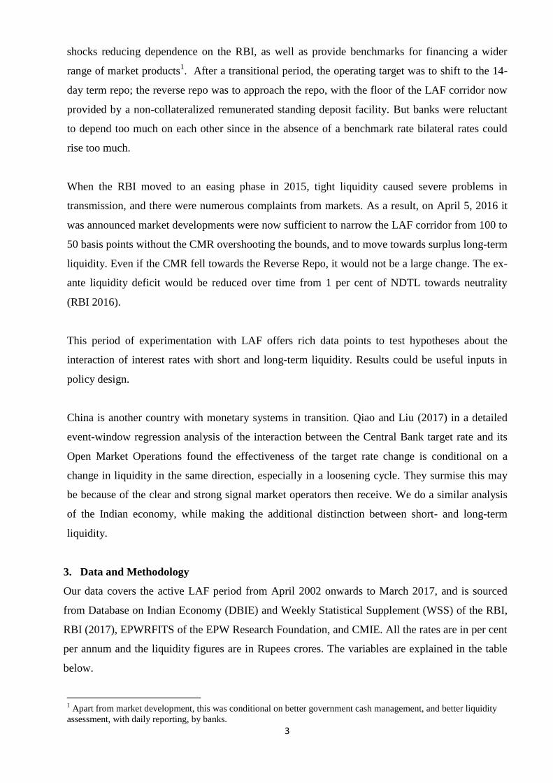
Table 2: Monthly Liquidity Operations

Phases Easing

Phase (Apr 02 to Oct

05)

Tightening

Phase (Nov 05 to Oct

08)

Easing

Phase (Nov 08 to Mar

10)

Tightening

Phase (Apr 10 to Apr

12)

Easing

Phase (May 12 to Sep

13)

Tightening

Phase (Oct 13 to Jan 15)

Easing

Phase (Feb 15 to Mar

17)

I II III IV V VI VII

Time Duration (months) 43 36 17 25 17 26 26

Change in Repo 8.00 to 6.00 6.00 to 9.00 9.00 to 4.75 4.75 to 8.5 8.5 to 7.25 7.25 to 8.00 8.00 to 6.25

No. of Times Changed 4 10 6 13 4 3 6

Basis Points -200 300 -425 325 -125 75 -175

LAF (Net Injection (+)/Absorption (-)) 6103872 -2317386 -23132185 26767905.5 25205282 6975521 -7439967

OMO (Net Purchase of Securities (+)/Sale

(-))

-94498 19018 150800 210796 177757.13 -34775 160453

Net RBI Intervention in Forex Market

(Net Purchase of Foreign Assets (+)/Sales

(-))

368228 671788 -128912 170138 246590 262350 405430

CRR Amount (Net Injection

(+)/Absorption (-))

-33138.00 -144369.00 -33378.00 -17327.00 -62695.00 11134.00 -180207.00

MSS (Net Injection (+)/Absorption (-)) -69255 -100250 166760 2737 0 0 0

Long Term Liquidity 171337.00 446187.00 155270.00 366344.00 361652.13 238709.00 385676.00

Total Liquidity 6275209 -1871199 -22976915 27134249.5 25566934.13 7214230 -7054291

Source : Self Computed using data sourced from EPWRFITS and DBIE

The duration of the cycles range from 25 months to as long as 43 months. The shortest phases

were III and V. Phase III was the post Global Financial Crisis (GFC) stimulus. The GDP growth

hit a decade low of 5 per cent in 2012-2013 (Phase V). RBI, therefore, followed an

accommodating monetary stance, which was reversed by the move towards inflation targeting.

Total Liquidity has been derived as a summation of Net Injections (+)/Absorptions (-) through

LAF, OMO, CRR, MSS and Forex market intervention. Long Term Liquidity is obtained by

subtracting LAF from Total Liquidity. Long Term Liquidity has remained in the net injection

mode throughout the period while Total Liquidity has both injection and absorption phases.

2 Dicky-Fuller unit root tests, of all the non-dummy variables used in the regressions, rejected the null hypotheses of

non-stationarity, validating the use of OLS.

6

Therefore LAF had a major impact on liquidity conditions in the economy. The policy rate and

different types of liquidity were not necessarily complementary to each other.

Liquidity and the Repo have often not worked in the same direction. Liquidity has not always

been surplus during easing phases, since the RBI was most often in the injection mode, denoting a

liquidity deficit, even during easing phases. Over 2010-15, this was a conscious decision. Between

2003 and 2009 large capital flows and the post GFC stimulus kept liquidity in surplus requiring

absorption regardless of the monetary cycle (Graph 1).

Irrespective of the phases, Long Term Liquidity saw net injections for most of the period, albeit at

low levels, to meet the needs of a growing economy (Graphs 2 and 3). The size of intervention

increased over the years with the size of the economy. It is interesting to observe the huge

liquidity absorption through Long Term Liquidity channels, in December 2016 following

demonetisation, after which liquidity was injected till March, 2017. This may have been due to the

high cost of sterilisation for the RBI using LAF and the decision to shift some of this burden to the

012345678910

-4000000

-3000000

-2000000

-1000000

0

1000000

2000000

3000000

4000000

Ap

r-0

2

Jan

-03

Oct

-03

Jul-

04

Ap

r-0

5

Jan

-06

Oct

-06

Jul-

07

Ap

r-0

8

Jan

-09

Oct

-09

Jul-

10

Ap

r-1

1

Jan

-12

Oct

-12

Jul-

13

Ap

r-1

4

Jan

-15

Oct

-15

Jul-

16

Rat

es

(%)

Vo

lum

e (

Rs

Cro

re)

Months

Graph 1: Total Liquidity vs Repo Rate: Monthly TotalLiquidity

RepoRate

Phase I Phase II III Phase IV V VI Phase VII

0

1

2

3

4

5

6

7

8

9

10

-600000

-500000

-400000

-300000

-200000

-100000

0

100000

200000

300000

400000

Ap

r-0

2

De

c-0

2

Au

g-0

3

Ap

r-0

4

De

c-0

4

Au

g-0

5

Ap

r-0

6

De

c-0

6

Au

g-0

7

Ap

r-0

8

De

c-0

8

Au

g-0

9

Ap

r-1

0

De

c-1

0

Au

g-1

1

Ap

r-1

2

De

c-1

2

Au

g-1

3

Ap

r-1

4

De

c-1

4

Au

g-1

5

Ap

r-1

6

De

c-1

6

Rat

es

(%)

Vo

lum

e (

Rs

Cro

re)

Months

Graph 2: Long Term Liquidity vs Repo Rate: Monthly LongTermLiquidity

RepoRate

Phase I Phase II III Phase IV V VI Phase VII

7

banking system, rather than due to changes in the demand for Long Term Liquidity. Total

Liquidity, however, was in absorption mode for the entire period after demonetisation.

Graph 3 shows Long Term and Total Liquidity for annual data. As with the high frequency data,

Long Term Liquidity is positive for the entire period while Total Liquidity switches from

injection to absorption with much higher amounts in the post GFC period. But injections shrink

over 2013-16. The absolute value of the ratio of Long Term Liquidity to Total Liquidity is very

low implying that LAF was the dominant source of short-term liquidity (Table 3).

Table 3: Annual Liquidity Operations

Phases Easing Phase

(2002-05)

Tightening

Phase (2005-08)

Easing Phase

(2008-10)

Tightening

Phase (2010-12)

Easing

Phase (2012-13)

Tightening

Phase (2013-14)

Easing Phase

(2014-17)


LAF (Net Injection

(+)/Absorption (-)

9364782 -7023996 -21779135 26160475.5 20469885 11250543 -4567497

OMO (Net Purchase of

Securities (+)/Sale (-))

-97898.77 -3115.26 170016.245 201310.33 154547 52290 122374.233

Net RBI Intervention in Forex

Market (Net Purchase

(+)/Sales (-)

344003 602902 -46373 180861 82119 248280 584030

CRR Amount (Net Injection

(+)/Absorption (-)

-22887.94 -92930.3898 -93979.4002 -132234.64 67217.967 35620.2212 -181154.8182

MSS (Net Injection

(+)/Absorption (-)

-64211 -104181 165655 2737 0 0 0

Long Term Liquidity 159005.29 402675.3502 195318.8448 252673.69 303883.967 336190.2212 525249.4148

Total Liquidity 9523787.29 -6621320.65 -21583816.16 26413149.19 20773768.97 11586733.22 -4042247.585

Source : Self Computed using data sourced from DBIE and EPWRFITS

3.2 Stylized facts: Repo Rate and Market Interest Rates

Larger alteration in Repo Rate causes most of the rates to move in the same direction (Table 4). In

Phases V and VI, which had the lowest adjustment compared to other phases, with the LAF in

deficit despite an easing cycle, the market rates did not adjust in the same direction as the Repo

Rate. Over the years, elasticity of adjustment of 91-Day T-Bills and to some extent 1-Year G-Sec

0

1

2

3

4

5

6

7

8

9

-25000000-20000000-15000000-10000000

-50000000

500000010000000150000002000000025000000

20

02

-03

20

03

-04

20

04

-05

20

05

-06

20

06

-07

20

07

-08

20

08

-09

20

09

-10

20

10

-11

20

11

-12

20

12

-13

20

13

-14

20

14

-15

20

15

-16

20

16

-17

Rat

es

(%)

Vo

lum

e (

Rs

Cro

re)

Years

Graph 3: Long Term & Total Liquidity vs Repo Rate: Annual Long TermLiquidity

TotalLiquidity

Year EndRepo Rate

Phase I Phase II Phase III IV

V VI Phase VII

8

increased in absolute terms but 10-Year G-Sec did not follow the same pattern. This suggests

long-term market rates may be influenced by other factors like present and future economic

activities, output gap, fiscal policy and the global environment (Kanagasabapathy et. al. 2016).

Among other rates, CD Rate (low), CP and Call Money Rate show good adjustment to changes in

the policy rate.

Table 4: Repo Rate and Market Interest Rates – Basis Points changes in the phases

Phases Easing

Phase

(Apr 02 to

Oct 05)

BPS Tight.

Phase (Nov

05 to Oct

08)

BPS Easing

Phase

(Nov 08 to

March 10)

BPS Tight.

Phase (Apr

10 to Apr

12)

BPS Easing Phase

(May 12 to

Sep 13)

BPS Tight.

Phase (Oct

13 to Jan

15)

BPS Easing

Phase

(Feb 15

to Mar

17)

BPS


Time

Duration

(months)

43 36 17 25 17 26 26

Change in

Repo

8.00-6.00 -200 6.00-9.00 300 9.00-4.75 -425 4.75-8.5 325 8.5-7.25 -125 7.25-8.00 75 8.00-6.25 -175

Change in

Call

Money

Market

Rate

6.51-5.12 -139 5.29-4.16 -113 6.78-3.34 -344 3.47-8.82 535 8.81-10.26 145 9.08-8.11 -97 7.88-6.04 -184

Change in

CD Rate

Low 5-4.66 -34 5.25-8.92 367 8.8-4 -480 4.52-9.34 482 9-9.37 37 9.16-8.3 -86 8.06-6.21 -185

High 10.88-

7.75

-313 7.75-21 -754 12.9-7.36 -554 7.12-12 488 10.6-11.95 135 11.95-8.67 -328 8.65- 6.7 -195

Change in

CP Rate

Low 7.6-5.69 -191 5.63-11.9 627 11.55-4 -755 5.3-8.51 321 8.02-8.17 15 9.5-7.98 -152 8.06-5.99 -207

High 11.1-7.5 -360 7.5-17.75 1025 16.9-8.9 -800 9-14.5 550 14.25-13.8 -45 13.57-12.61 -96 11.73-

13.33

160

Change in

CBLO

3.55-5.09

(From

Jan'04)

154 5.05-4.08 -97 5.32-3.27 -205 3.05-8.5 545 8.39-10.22 183 7.76-8.32 56 8.02-5.5 -252

Change in

91 Day TB

5.85-5.47 -38 5.41-7.43 202 7.05-4.3 -275 4.25-8.59 434 8.37-9.9 153 9.84-8.15 -169 7.92-6.06

(till Feb

'17)

-186

Change in

1 Year G-

Sec

5.68-5.78 10 5.8-7.8 200 7.47-5.38 -209 5.25-8.12 -287 7.97-9.58 161 12.29- 8.01 -428 7.77-6.36

(till Feb

'17)

-141

Change in

10 Year G-

Sec

7.23-7.14 -9 7.14-7.73 59 7.85-7.88 3 7.87-8.50 -63 8.45-8.18 -27 8.35-7.98 -37 7.88-7.43

(till Feb

'17)

-45

Change in

Bank PLR

/Base Rate

Low 11-10.25 -75 10.25-13.75 350 13-11 -200 11-10 -100 10-9.8 -20 10-10 0 10-9.25 -75

High 12-10.75 -125 10.75-14 325 13.5-12 -150 12-10.75 -125 10.5-10.25 -25 10.25-10.25 0 10.25-9.6 -65

Source: Self Computed using data from EPWRFITS and DBIE

Surplus liquidity meant the overnight call money market rate stayed closer to the reverse Repo

Rate until 2010, after which the deficit mode kept it closer to the Repo Rate. Large exogenous

shocks that could not be smoothed meant it overshot the LAF bounds, although this became rarer

over the years. Indicative bank lending rates are also shown in Graph 4. The Prime Lending Rate

(PLR), which is closer to an upper bound is graphed until July 2010 and the Base Rate, closer to a

minimum rate after. That is why the gap between the Repo Rate and the bank lending rate shrinks.

Bank lending rates also follow the Repo Rate, but less than market rates do and generally more

during tightening compared to loosening episodes (Table 4). The weighted average lending rate

(WALR) for all commercial banks, shown for the period after February 2012 lies above the Base

9

Rate. While the Base Rate did not rise with the Repo Rate in the tightening phase VI, the WALR

continued to fall. It has been falling since 2013, perhaps reflecting poor demand for loans. It is not

true that the current monetary loosening has not transmitted to banks, although the gap between

the Base Rate, the WALR and the Repo increased in 2016 that between the Base Rate and the

WALR fell.

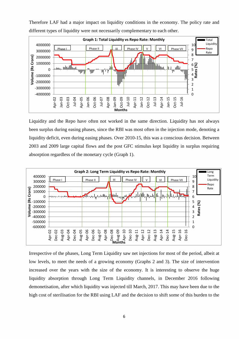
Other rates show a similar picture with some variations. CP rates adjusted closely within the repo

and reverse repo band over the years. It failed to stay in the window from 2006-2012 possibly

because of surplus liquidity and then reduced demand. But it reached the top of the LAF band by

2014 (Graph 5). The CBLO rates reached and sometimes exceeded the top of the LAF band in the

liquidity deficit period of 2012 (Graph 6).

0

2

4

6

8

10

12

14

16

Ap

r-0

2

De

c-0

2

Au

g-0

3

Ap

r-0

4

De

c-0

4

Au

g-0

5

Ap

r-0

6

De

c-0

6

Au

g-0

7

Ap

r-0

8

De

c-0

8

Au

g-0

9

Ap

r-1

0

De

c-1

0

Au

g-1

1

Ap

r-1

2

De

c-1

2

Au

g-1

3

Ap

r-1

4

De

c-1

4

Au

g-1

5

Ap

r-1

6

De

c-1

6

Rat

es

(%)

Months

Graph 4: Repo & Reverse Repo Rate vs Call Market Rate RepoRate

ReverseRepoRateCallmoney

PLR/BaseRate

WALR AllSCBs

Phase I Phase II Phase III Phase IV V VI Phase VII

10

0

1

2

3

4

5

6

7

8

9

20

01

-02

20

02

-03

20

03

-04

20

04

-05

20

05

-06

20

06

-07

20

07

-08

20

08

-09

20

09

-10

20

10

-11

20

11

-12

20

12

-13

20

13

-14

20

14

-15

20

15

-16

20

16

-17

Rat

es

(%)

Years

Graph 5: Repo & Reverse Repo Rate vs CP CP

Repo

Reverserepo

0

1

2

3

4

5

6

7

8

9

20

08

-09

20

09

-10

20

10

-11

20

11

-12

20

12

-13

20

13

-14

20

14

-15

20

15

-16

20

16

-17

Rat

es

(%)

Years

Graph 6: Repo & Reverse Repo Rate vs CBLO CBLO

Repo

Reverserepo

0

1

2

3

4

5

6

7

8

9

20

01

-02

20

02

-03

20

03

-04

20

04

-05

20

05

-06

20

06

-07

20

07

-08

20

08

-09

20

09

-10

20

10

-11

20

11

-12

20

12

-13

20

13

-14

20

14

-15

20

15

-16

20

16

-17

Rat

es

(%)

Years

Graph 7: Repo & Reverse Repo vs CD CD

RepoRate

ReverseRepo

11

Before 2010, CD rates were erratic, and did not respond much to the policy rate changes (Graph

7). After 2010, it rose along with the policy rate and is in tune with the Repo Rate in the recent

years.

4. Analysis

We next turn to regression analysis of T and T±5 event windows of Repo Rate change. In our

baseline model, we take change in the Repo Rate as our primary independent variable and see if

its coefficient is significant on regressing with change in other market rates. Then we check if

there exists any asymmetry in pass through between increase and decrease in Repo Rate. Next we

try to analyse the efficacy of pass through when LAF is in injection mode and when Total

Liquidity is in absorption mode, denoting liquidity deficit3. We also assess the relative

effectiveness of short versus long run liquidity and how a Total Liquidity relative to LAF variable

performs. Last, we see if transmission is better when quantity variables are in sync with the Repo

Rate.

The Repo Rate has changed 56 times in the period under consideration. So T period regressions

have few data points. T±5 event window has more than 500 observations and also allows us to

investigate slightly longer-run market reactions. Table 5 gives the summary statistics. CMR,

CBLO are change in Call Money Market Rate and CBLO respectively; _91D is the change in 91-

Day T-Bills rate; _1Y, _10Y are the changes in yield of G-Secs of maturities 1-Year and 10-

Years; DRepo is the Repo Rate change around announcement dates, LRL is Long Run Liquidity,

and TL is Total Liquidity.

On an average, Repo Rate changed by -3.30 bps. Table 6 shows pairwise correlation between the

variables used in the analysis. All the market rates are positively correlated with DRepo.

Similarly, we observe positive correlation between the rates and quantity variables except for

Long Run Liquidity with 10-Year G-Secs. The correlation between yield curves and call money

rates, however, is negative. Our regression analysis will investigate the significance of these

correlations.

Our baseline model (Model 1) is –

3 Liquidity is injected in the LAF during deficit periods. So although the transaction itself reduces liquidity it is used

in the regressions to capture periods of short-term liquidity deficit. The absorption mode or OMO sale of G-Secs is

used to indicate liquidity tightening since it directly reduces money supply.

12

Table 7 shows the results of the baseline regression. We observe that all rates except 91-day T-

Bills and CMR reacts significantly to a change in Repo Rate for the T period regression.

However, 91-day T-Bills alone react significantly for the longer window. The strongest and most

immediate impact is on CLBO rates. The significance and the magnitude of Repo influence

increases with maturity, for T-Bills and G-Secs. One bps increase in DRepo increases _10Y and

_1Y G-Sec yields by 1.018 bps and 0.903 bps respectively in T, while 91-day T-Bills rate rises

0.186 bps only in T±5.

We use dummies to distinguish between periods of DRepo increase or decrease. Policy Rate

dummy R_D is set to be 1 if DRepo increases and 0 otherwise. Table 8 gives results on direction

of Repo Rate changes using the dummy variable. We observe that R_D is quite significant for

both the event windows, but it is significant for more rates in the T window with relatively higher

coefficients. The conclusion follows that transmission is faster during tightening. Now, we

introduce slope and intercept dummies in our baseline model to further test for asymmetry

between policy rate increase and decrease, while controlling for the change in the Repo itself. So

we will estimate the following Model 2 for each market rate studied4:

Model 2

Second, we try to assess the additional impact of quantum channels on transmission. For this we

take LAF_V_D as 1 if LAF is in injection mode and 0 otherwise in Model 3. TL_V_D is 1 if

Total Liquidity (TL) is in absorption mode and it is 0 otherwise in Model 4.

Model 3

Model 4

Table 9 for CMR reveals no significant difference from the baseline model for all the three

models. None of the coefficients are significant. The graphs showed us that the CMR was aligned

with the Repo Rate only under LAF deficit, but the LAF_V_D is not significant. These results do

not support the RBI (2011) view, that pass through is most rapid for the CMR since it reflects

demand by liquidity constrained banks.

4 As a robustness exercise, the models below were regressed through the origin and the results obtained were similar

to OLS regressions.

13

Table 10 shows the results for CBLO market. Only T window coefficients are significant, again

supporting immediate impact of DRepo on CBLO rates. The DRepo coefficients continue to be

strongly significant, while the R_D is not. The interaction of the Repo Dummy is insignificant

revealing that CBLO rates respond to Repo Rate increase or decrease in a similar manner, when

DRepo is included. However, the interaction with LAF Dummy and TL Dummy is significant.

CBLO falls when LAF liquidity is being injected but rises when Total Liquidity is being drained

in absorption mode. Thus changes in liquidity matter or the quantum channel adds to the rate

channel. Repo Rate changes dominates the direction effect of Repo Rate increase.

Table 11 displays the results for 91-day Treasury Bills market. The interaction dummies are

significant as is the Repo dummy in the T event window. The market reacts to Repo Rate

increasing operations and liquidity injecting operations (considering both LAF and TL) to a larger

extent. But DRepo has a stronger impact compared to quantity change dummies. The significant

coefficient for R_D in T±5 is negative, moreover, suggesting that the rate falls during tightening

when the Repo Rate is rising.

Table 12 shows that the interactions are not significant for either event windows for 1-Year G-

Secs. Only the DRepo coefficient is significant. There is no asymmetry and the quantum channel

does not add to transmission. The T period DRepo coefficients are larger suggesting immediate

impact of a policy rate change.

Table 13 for 10-Year G-Secs shows significant coefficients for DRepo in T. This responds fast

perhaps since it is the deepest G-sec market. Of the dummy variables only TL dummy is

significant in T, suggesting that long-run liquidity matters for a rate that gives the markets view of

longer-term prospects.

Although the volume and volume interaction dummies are rarely significant in models 3 and 4,

the controls for the quantum channels increase the size of the DRepo coefficients, compared to the

baseline model, suggesting the quantum channel increases the impact of a change in the Repo

Rate. Next we investigate results for settings when liquidity and repo changes work in sync with

each other, that is, when liquidity changes are in the same direction as Repo Rate changes. For

example, for periods when the Repo Rate is rising so R_D equals one, we take the periods when

the LAF was in injection mode and the TL in absorption mode as indicated by the dummy

14

variables. The relevant coefficients under four different combinations of Repo, LAF and TL

change are listed in Table 14(A) and (B). The models used are –

Model 5

Model 6

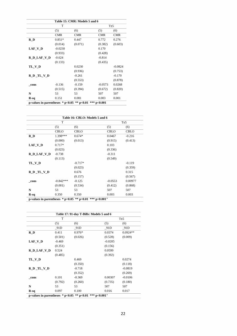
For the first time, the R_D coefficient is significant for CMR in T (Model 5, Table 15), pointing to

the impact of a LAF channel in sync for transmission from CMR. Only for 1-Year G-Secs is an

interaction dummy significant and positive, suggesting that transmission is better in T±5 under

tightening when the LAF is in injection mode (Table 18). While R_D coefficients are often

significant, the only other quantity dummy significant is a negative impact of total liquidity

reduction on CLBO rates in T (Table 16), but a positive impact on 10-Year G-Secs rates in T±5.

The significant constant term for CBLO suggests it responds to monetary loosening also.

Lastly, all the markets respond more to monetary tightening (and loosening for CLBO and 10

Year G-Secs, where the coefficient is significant) when quantity controls are included. This again

suggests that quantity variables intensify the pass through of Repo Rate changes.

To assess the relative effect of short-versus long-run liquidity, we will now insert the ratios

LAF/TL and LAF/LRL one by one to the baseline model where LRL stands for Long Run

Liquidity. We define LR1 = LAF/TL and LR2 = LAF/LRL as the two Liquidity Ratios. The new

models are –

Model 7

Model 8

Tables 20-21 show results for those of the above models, where liquidity ratios are significant.

These are only the negative impact of LR1 on CMR in T (Table 20)5 and its positive impact on

10-Year G-Secs in T±5. When LR1 increases, CMR decreases by 2.31 units and 10-Year G-Sec

yield increases by 0.004 units. It is interesting that this is only the second significant coefficient

obtained for CMR, and like Model 5 (Table 15), suggests that it is affected by relative short-run

5 When regressed through origin (RTO), LR1 was no longer significant for CMR; all the other results remained the

same.

15

liquidity, falling when LAF injections are relatively high. The positive LR1 coefficient for 10-

Year G-Sec supports the result frequently obtained that LR liquidity is important for 10-Year G-

Secs so that a relative rise in short-run liquidity raises yields. DRepo is significant for some rates,

which further supports the dominant role of the interest rate channel.

Finally, we draw out implications of the results, for the questions we posed. The speed of

transmission is fastest for CBLO and 10-Year G-Secs markets that have more depth, while it is

slowest in the 91-day T-Bills market. Table 1 shows the turnover is more for CBLO than for Call

Money Market, and more for G-Secs compared to T-bills. Thin markets are more dependent on

RBI liquidity provision. CMR shows least transmission although RBI (2011) wanted it to be the

instrument variable. Our results suggest CLBO would now be a better rate to target.

Analysis with dummies reveals that only 10-Year G-Secs yield is affected by absorption through

Total Liquidity channel, and only 91-day T-Bills yield is affected by Repo Rate changing

direction, responding more to rate increases. Its relative market depth makes the 10-Year G-Secs

yield respond fast to short-term policy rate changes, but the impact of the long-run factors

Kanagasabapathy et. al. (2014) found more important comes in through the impact of long-run

liquidity.

5. Conclusion

This paper uses simple OLS regressions of event windows around change in Repo Rates to

explore the relative performance and interaction of rate and quantity channels in Indian monetary

transmission. The results find the interest rate channel, with Repo Rate as the policy rate, as the

most effective medium to influence market rates. Over the years, RBI has been quite successful in

controlling the market rates through adjustments in Repo and Reverse Repo Rates. After 2012, the

market rates have operated within the corridor defined by the Repo and Reverse Repo rates.

The interest rate transmission channel is dominant, but controlling for the liquidity channel

increases the impact of the Repo Rate, especially for the rates where markets are thin. So the

quantity channel has an indirect impact. The speed of response is faster where there is more

market depth. Short term liquidity matters for short term rates, especially where markets are thin

and long-term liquidity for longer term government securities. Asymmetry, or better transmission

during tightening, finds little support, except for faster pass through during tightening. Market

rates respond similarly to policy rate changing direction. The quantum channel directly

16

contributes more when it works in sync with the interest rate channel only for 1-year G-Secs and

the CMR, but contributes indirectly by increasing the size of rate change coefficients.

What are the implications for current policy positions and research conclusions? Our results do

not support the current RBI practice of keeping the CMR as the intermediate target. This is

especially so if quantity and rate variables are not in sync. The CLBO Rate responds most and

fastest to a change in the Repo Rate, because of the largest turnover in this market (Table 1).

Similarly the 10-Year G-Sec responds fastest because of greater market depth but the long run

variables that the literature finds affect this variable come in through the impact on it of long-run

liquidity. Our results also do not support the recommendation of RBI (2011) that transmission is

fastest when liquidity is in deficit, since the size of pass through rises if rate and quantity variables

are in sync. Table 4 also shows that during the easing phase V (May 2012 to Sept. 2013) when

liquidity was in deficit market rates did not follow the Repo Rate down. Liquidity provision

matters more in thin markets. Therefore the current move away from maintaining liquidity in

deficit, even while narrowing the LAF corridor, is in the right direction.

Possible extensions include examining the role of the term Repo markets and outcome in windows

longer than T and T±5. Transmission to bank lending rates is of major interest, and needs rigorous

analysis. It requires alternative approaches, however, since it cannot be captured in five and

twenty day windows. Since the two are linked (Graph 4), and policy seeks to further increase their

sensitivity to market rates, improving transmission to market rates will also improve that to bank

lending rates.

References

Goyal, A. 2017. ‘Monetary Policy Transmission in India,’ Chapter 3 in S. Mahendra Dev (ed.),

India Development Report 2017, pp. 35-48, New Delhi: IGIDR and Oxford University Press.

Kanagasabapathy, K., R. A. Bhangaonkar, and S. R. Pandey. 2014. ‘Monetary Policy

Transmission in India: Interplay of Rate and Quantum Channels,’ chapter 6 in Goyal, A. (ed.) A

Concise Handbook of the Indian Economy in the 21st Century. OUP Catalogue.

Khundrakpam, J. K. and R. Jain. 2012. ‘Monetary Policy Transmission in India: A Peep Inside the

Black Box,’ RBI working paper series no. 11. Available at

https://www.rbi.org.in/scripts/PublicationsView.aspx?id=14326.

Qiao, Z. and Y. Liu. 2017. ‘Open Market Operation Effectiveness in China,’ Emerging Markets

Finance and Trade, 53(8), pp. 1706-1719.

RBI (Reserve Bank of India). 2011. ‘Report of the Working Group on Operating Procedures of

Monetary Policy,’ 15th

March: Website:

https://www.rbi.org.in/scripts/PublicationReportDetails.aspx?ID=631

17

RBI. 2014. ‘Report of the Expert Committee to Revise and Strengthen the Monetary Policy

Framework,’ January. Website:

https://rbidocs.rbi.org.in/rdocs/PublicationReport/Pdfs/ECOMRF210114_F.pdf

RBI. 2016. ‘Reserve Bank of India Annual report 2015-16’. Website:

https://www.rbi.org.in/Scripts/AnnualReportPublications.aspx?year=2016

RBI. 2017. Handbook of Statistics on Indian Economy: Website: http://www.rbi.org.in

18

Appendix

Table 5: Summary Statistics

Variable Mean Std. Dev. Min Max

CMR 0.0464151 0.7261015 -1.18 4.7

CBLO 0.065283 0.9288715 -2.95 2.35

_91D 0.197883 1.283596 -1.8548 7.0458

_1Y -0.0356038 1.003339 -3.532 4.842

_10Y -0.012434 0.6808206 -1.474 2.38

DRepo -0.0330189 0.4788752 -1 1.75

LAF 20692 49678.65 -96615 145365

LRL 1323.811 5760.611 -10326 30398

TL 22015.81 51162.56 -96615 145365

Total Observations = 53

Table 6: Pairwise Correlation

CMR CBLO _91D _1Y _10Y DRepo LAF LRL TL

CMR 1

CBLO 0.1311 1

_91D 0.1572 0.0364 1

_1Y -0.0582 0.3608 0.1666 1

_10Y -0.0179 0.5268 0.1612 0.3362 1

DRepo 0.1907 0.5983 0.2604 0.4312 0.7161 1

LAF 0.0034 0.1867 0.0354 0.1723 0.0876 0.2968 1

LRL 0.4001 0.0784 0.0797 0.1654 -0.1497 0.0712 0.2035 1

TL 0.0483 0.1901 0.0433 0.186 0.0682 0.2962 0.9939 0.3102 1

Table 7: Baseline Model

T T±5

N=53 N=507

DRepo _cons DRepo _cons R-sq

(1) CMR 0.289 0.0560 0.325 0.0232 0.0003

(0.171) (0.575) (0.683) (0.821)

(2) CBLO 1.161*** 0.104 -0.0202 -0.0221 0

(0.000) (0.321) (0.959) (0.665)

(3) _91D 0.698 0.221 0.186*** -0.000569 0.0237

(0.060) (0.206) (0.001) (0.934)

(4) _1Y 0.903** -0.00577 0.126 -0.000590 0.0074

(0.001) (0.964) (0.053) (0.944)

(5) _10Y 1.018*** 0.0212 0.0436 0.00366 0.0018

(0.000) (0.750) (0.337) (0.530)

p-values in parentheses *p<0.05 **p<0.01 ***p<0.001

Table 8: Model with only Repo Dummy

T T±5

N=53 N=507

R_D _cons R_D _cons R-sq

(1) CMR 0.385 -0.150 0.234 0.0100 0.0005

(0.053) (0.285) (0.614) (0.924)

(2) CBLO 0.968*** -0.428** -0.146 -0.0145 0.0008

(0.000) (0.009) (0.527) (0.781)

(3) _91D 0.722* -0.170 0.0743* -0.00502 0.0111

(0.039) (0.488) (0.018) (0.477)

(4) _1Y 0.566* -0.324 0.113** -0.00681 0.0174

(0.039) (0.095) (0.003) (0.426)

(5) _10Y 0.711*** -0.375** 0.0156 0.00271 0.0007

(0.000) (0.002) (0.555) (0.650)

p-values in parentheses *p<0.05 **p<0.01 ***p<0.001

19

Table 10: CBLO: Models 2, 3 and 4

T T±5

(2) (3) (4) (2) (3) (4)

Variables CBLO CBLO CBLO CBLO CBLO CBLO

DRepo 1.153* 1.819*** 0.746** 0.141 0.0226 -0.0894

(0.043) (0.000) (0.007) (0.768) (0.968) (0.872)

R_D 0.203 -0.317

(0.574) (0.676)

DRepo _R_D -0.344 0.442

(0.649) (0.862)

LAF_V_D 0.0991 0.0784

(0.662) (0.451)

DRepo _LAFVD -1.084* -0.121

(0.023) (0.880)

TL_V_D -0.138 -0.104

(0.560) (0.417)

DRepo _TLVD 1.032* 0.0687

(0.034) (0.932)

_cons 0.0599 0.106 0.217 0.0118 -0.0540 0.000610

(0.830) (0.578) (0.081) (0.824) (0.420) (0.992)

N 53 53 53 507 507 507

R-sq 0.366 0.435 0.433 0.001 0.001 0.001

p-values in parentheses * p<0.05 ** p<0.01 *** p<0.001"

Table 9: CMR: Models 2, 3 and 4

T T±5

(2) (3) (4) (2) (3) (4)

Variables CMR CMR CMR CMR CMR CMR

DRepo -0.160 0.719 0.335 0.128 0.292 0.578

(0.761) (0.059) (0.220) (0.893) (0.798) (0.604)

R_D 0.475 -0.0318

(0.167) (0.983)

DRepo 0.0940 0.785

(0.895) (0.878)

LAF_V_D -0.398 0.144

(0.079) (0.491)

DRepo _LAFVD -0.499 -0.00108

(0.278) (0.999)

TL_V_D -0.123 -0.0880

(0.606) (0.732)

DRepo _TLVD -0.233 -0.584

(0.631) (0.717)

_cons -0.217 0.354 0.0784 0.0125 -0.0363 0.0383

(0.412) (0.063) (0.528) (0.907) (0.787) (0.739)

N 53 53 53 507 507 507

R-sq 0.074 0.103 0.044 0.001 0.001 0.001

p-value in parenthesis * p<0.05 ** p<0.01 *** p<0.001

20

Table 11: 91-day T-Bills: Models 2, 3 and 4

T T±5

(2) (3) (4) (2) (3) (4)

Variables _91D _91D _91D _91D _91D _91D

DRepo -0.888 -0.300 1.351** 0.130* 0.0128 0.363***

(0.325) (0.641) (0.004) (0.041) (0.865) (0.000)

R_D 0.694 -0.255*

(0.237) (0.012)

DRepo _R_D 2.068 1.002**

(0.094) (0.003)

LAF_V_D -0.114 -0.0148

(0.767) (0.282)

DRepo _LAFVD 1.625* 0.349**

(0.043) (0.001)

TL_V_D -0.0388 0.0253

(0.922) (0.134)

DRepo _TLVD -1.845* -0.346**

(0.024) (0.001)

_cons -0.546 0.194 0.107 -0.00252 0.00408 -0.00737

(0.230) (0.547) (0.602) (0.721) (0.645) (0.331)

N 53 53 53 507 507 507

R-sq 0.135 0.156 0.167 0.041 0.047 0.050


Table 12: 1-Year G-Secs: Models 2, 3 and 4

T T±5

(2) (3) (4) (2) (3) (4)

Variables _1Y _1Y _1Y _1Y _1Y _1Y

DRepo 1.186 1.033* 0.732* 0.0391 0.0187 0.228*

(0.084) (0.039) (0.036) (0.616) (0.841) (0.013)

R_D -0.357 0.151

(0.417) (0.223)

DRepo_R_D 0.0432 -0.174

(0.962) (0.676)

LAF_V_D 0.200 0.00197

(0.493) (0.908)

DRepo_LAFVD -0.295 0.211

(0.622) (0.107)

TL_V_D -0.181 0.000705

(0.551) (0.973)

DRepo_TLVD 0.321 -0.209

(0.600) (0.111)

_cons 0.178 -0.121 0.0722 -0.00606 -0.00230 -0.00144

(0.601) (0.620) (0.645) (0.486) (0.834) (0.878)

N 53 53 53 507 507 507

R-sq 0.197 0.202 0.201 0.018 0.013 0.012

p-values in parentheses * p<0.05 ** p<0.01 *** p<0.001

21

Table 13: 10-Year G-Secs: Models 2, 3 and 4

T T±5

(2) (3) (4) (2) (3) (4)

Variables _10Y _10Y _10Y _10Y _10Y _10Y

DRepo 1.030** 1.128*** 1.033*** 0.0308 0.0207 0.0704

(0.005) (0.000) (0.000) (0.572) (0.750) (0.266)

R_D -0.175 -0.0766

(0.445) (0.376)

DRepo _R_D 0.286 0.287

(0.551) (0.324)

LAF_V_D -0.211 -0.0114

(0.168) (0.336)

DRepo _LAFVD -0.0789 0.0506

(0.799) (0.578)

TL_V_D 0.317* 0.0269

(0.043) (0.065)

DRepo _TLVD 0.232 -0.0361

(0.456) (0.693)

_cons 0.0610 0.167 -0.0613 0.00331 0.00817 -0.00199

(0.731) (0.191) (0.442) (0.587) (0.285) (0.761)

N 53 53 53 507 507 507

R-sq 0.524 0.532 0.552 0.004 0.004 0.009


Table 14(A): Possible combinations of LAF and Repo Rate changes

DRepo>0 DRepo<0

Coefficients Interpretation Coefficients Interpretations

LAF>0 Constant + R_D + LAF_V_D +

(R_D*LAF_V_D)

Increase in Repo Rate during LAF injection

Constant + LAF_V_D Decrease in Repo Rate during LAF injection

LAF<0 Constant + R_D Increase in Repo Rate during LAF

absorption

Constant Decrease in Repo Rate during

LAF absorption

Table 14(B): Possible combinations of Total Liquidity and Repo Rate changes

DRepo>0 DRepo<0

Coefficients Interpretation Coefficients Interpretations

TL<0 Constant + R_D + TL_V_D +

(R_D*TL_V_D)

Increase in Repo Rate during TL absorption

Constant + TL_V_D Decrease in Repo Rate during TL absorption

TL>0 Constant + R_D Increase in Repo Rate during

TL injection

Constant Decrease in Repo Rate

during TL injection

22

Table 15: CMR: Models 5 and 6

T T±5

(5) (6) (5) (6)

CMR CMR CMR CMR

R_D 0.851* 0.447 0.772 0.276

(0.014) (0.071) (0.382) (0.603)

LAF_V_D -0.0230 0.170

(0.933) (0.428)

R_D_LAF_V_D -0.624 -0.814

(0.133) (0.435)

TL_V_D 0.0230 -0.0824

(0.936) (0.753)

R_D _TL_V_D -0.261 -0.170

(0.553) (0.878)

_cons -0.136 -0.159 -0.0573 0.0268

(0.515) (0.394) (0.672) (0.820)

N 53 53 507 507

R-sq 0.151 0.081 0.003 0.001


Table 16: CBLO: Models 5 and 6

T T±5

(5) (6) (5) (6)

CBLO CBLO CBLO CBLO

R_D 1.398*** 0.674* 0.0467 -0.216

(0.000) (0.013) (0.915) (0.413)

LAF_V_D 0.717* 0.103

(0.023) (0.336)

R_D_LAF_V_D -0.738 -0.311

(0.113) (0.549)

TL_V_D -0.717* -0.119

(0.023) (0.359)

R_D _TL_V_D 0.676 0.315

(0.157) (0.567)

_cons -0.842*** -0.125 -0.0553 0.00977

(0.001) (0.534) (0.412) (0.868)

N 53 53 507 507

R-sq 0.350 0.350 0.003 0.003


Table 17: 91-day T-Bills: Models 5 and 6

T T±5

(5) (6) (5) (6)

_91D _91D _91D _91D

R_D 0.411 0.976* 0.0374 0.0924**

(0.501) (0.026) (0.528) (0.009)

LAF_V_D -0.469 -0.0205

(0.351) (0.156)

R_D_LAF_V_D 0.524 0.0599

(0.485) (0.392)

TL_V_D 0.469 0.0274

(0.350) (0.118)

R_D _TL_V_D -0.718 -0.0819

(0.352) (0.269)

_cons 0.101 -0.369 0.00307 -0.0106

(0.792) (0.260) (0.735) (0.180)

N 53 53 507 507

R-sq 0.097 0.100 0.016 0.017


23

Table 18: 1-Year G-Secs: Regression results for Models 5 and 6

T T±5

(5) (6) (5) (6)

_1Y _1Y _1Y _1Y

R_D 0.575 0.452 -0.0150 0.153***

(0.228) (0.176) (0.834) (0.000)

LAF_V_D 0.434 -0.0118

(0.267) (0.497)

R_D_LAF_V_D -0.107 0.180*

(0.853) (0.033)

TL_V_D -0.434 0.00663

(0.267) (0.754)

R_D _TL_V_D 0.122 -0.173

(0.838) (0.054)

_cons -0.574 -0.141 -0.00213 -0.00816

(0.056) (0.579) (0.846) (0.394)

N 53 53 507 507

R-sq 0.114 0.113 0.026 0.025


Table 19: 10-Year G-Secs: Models 5 and 6

T±5 T

(5) (6) (5) (6)

_10Y _10Y _10Y _10Y

R_D -0.0190 0.0312 0.872** 0.600**

(0.705) (0.300) (0.004) (0.004)

LAF_V_D -0.0144 0.0830

(0.239) (0.726)

R_D_LAF_V_D 0.0539 -0.236

(0.363) (0.506)

TL_V_D 0.0294* -0.0830

(0.048) (0.723)

R_D _TL_V_D -0.0709 0.425

(0.258) (0.240)

_cons 0.00841 -0.00327 -0.422* -0.339*

(0.275) (0.625) (0.022) (0.029)

N 507 507 53 53

R-sq 0.004 0.009 0.285 0.302


Table 20: CMR: Models 7 and 8

T T±5

(7) (8) (7) (8)

CMR CMR CMR CMR

DRepo 0.234 0.846 0.331 1.633

(0.162) (0.814) (0.737) (0.832)

LR1 -2.309*** 0.00551

(0.000) (0.849)

LR2 -0.435 0.00434

(0.333) (0.880)

_cons 2.234*** 1.611 0.0439 0.301

(0.000) (0.311) (0.789) (0.609)

N 53 6 318 81

R-sq 0.412 0.339 0.000 0.001


24

Table 21: 10-Year G-Secs: Models 7 and 8

T T±5

(7) (8) (7) (8)

_10Y _10Y _10Y _10Y

DRepo 1.018*** 0.985 0.0441 0.0129

(0.000) (0.540) (0.438) (0.973)

LR1 0.0102 0.00409*

(0.977) (0.015)

LR2 -0.0104 0.000476

(0.953) (0.739)

_cons 0.0115 0.0779 0.00120 0.0247

(0.973) (0.901) (0.899) (0.397)

N 53 6 318 81

R-sq 0.513 0.145 0.021 0.001


Tables

Table 1: Growth in Money and Government Securities Market – Start, Middle and End of the

Period under study

Table 2: Monthly Liquidity Operations

Table 3: Annual Liquidity Operations

Table 4: Repo Rate and Market Interest Rates – Basis Points changes in the phases

Table 5: Summary Statistics

Table 6: Pairwise Correlation

Table 7: Baseline Model Regression results

Table 8: Regression results for Model with only Repo Dummy

Table 9: CMR: Regression results for models 2, 3 and 4

Table 10: CBLO: Regression results for models 2, 3 and 4

Table 11: 91-day T-Bills: Regression results for models 2, 3 and 4

Table 12: 1-Year G-Secs: Regression results for models 2, 3 and 4

Table 13: 10-Year G-Secs: Regression results for models 2, 3 and 4

Table 14(A): Possible combinations of LAF and Repo Rate changes

Table 14(B): Possible combinations of Total Liquidity and Repo Rate changes

Table 15: CMR: Regression results for models 5 and 6

Table 16: CBLO: Regression results for models 5 and 6

Table 17: 91-day T-Bills: Regression results for models 5 and 6

Table 18: 1-Year G-Secs: Regression results for models 5 and 6


Table 20: CMR: Regression results for models 7 and 8


25

Graphs

Graph 1: Total Liquidity vs Repo Rate: Monthly

Graph 2: Long Term Liquidity vs Repo Rate: Monthly

Graph 3: Long Term & Total Liquidity vs Repo Rate: Annual

Graph 4: Repo & Reverse Repo Rate vs Call Money Market Rate

Graph 5: Repo & Reverse Repo Rate vs CP

Graph 6: Repo & Reverse Repo Rate vs CBLO

Graph 7: Repo & Reverse Repo Rate vs CD

Documents

Monetary transmission in India: Working of price and