Monetary Policy in Low Income Countries in the Face of the Global Crisis: The Case of

Zambia

Alfredo Baldini, Jaromir Benes, Andrew Berg, Mai C. Dao, Rafael Portillo

WP/12/94

© 2012 International Monetary Fund WP/12/94

IMF Working Paper

Research Department and African Department

Monetary Policy in Low Income Countries in the Face of the Global Crisis: The Case of Zambia *

Prepared by Alfredo Baldini, Jaromir Benes, Andrew Berg, Mai C. Dao, Rafael Portillo

Authorized for distribution by Andrew Berg and George Tsibouris

April 2012

Abstract

We develop a DSGE model with a banking sector to analyze the impact of the financial crisison Zambia and the role of the monetary policy response. We view the crisis as a combinationof three related shocks: a worsening in the terms of the trade, an increase in the country’s riskpremium, and a decrease in the risk appetite of local banks. We characterize monetary policy as “stop and go”: initially tight, subsequently loose. Simulations of the model broadly match the path of the economy during this period. We find that the initial policy response contributed to the domestic impact of the crisis by further tightening financial conditions. Westudy the factors driving the “stop” part of policy and derive policy implications for central

banks in low-income countries.

JEL Classification Numbers:E5, F32, F37

Keywords: Global Financial Crisis, Low-Income Countries, Monetary Policy, Zambia

Author’s E-Mail Address: abaldini@imf.org, jbenes@imf.org, aberg@imf.org, mdao@imf.org, rportillo@imf.org

* This working paper is part of a research project on macroeconomic policy in low-income countries supported by the U.K.’s Department for International Development.

This Working Paper should not be reported as representing the views of the IMF. The views expressed in this Working Paper are those of the author(s) and do not necessarily represent those of the IMF or IMF policy, or of DFID. Working Papers describe research in progress by the author(s) and are published to elicit comments and to further debate.

Contents

Page

I Introduction . . . . . . . . . . . . . . . . . . . . . . . . . . . . . . . . . . . . . . 4

II Core model structure . . . . . . . . . . . . . . . . . . . . . . . . . . . . . . . . . 7A Households . . . . . . . . . . . . . . . . . . . . . . . . . . . . . . . . . . . 8B Firms . . . . . . . . . . . . . . . . . . . . . . . . . . . . . . . . . . . . . . 9

1 Domestic Firms . . . . . . . . . . . . . . . . . . . . . . . . . . . . . 92 Exporting Firms . . . . . . . . . . . . . . . . . . . . . . . . . . . . . 10

C The Banking Sector . . . . . . . . . . . . . . . . . . . . . . . . . . . . . . . 11D Monetary Authority . . . . . . . . . . . . . . . . . . . . . . . . . . . . . . . 12E The Government . . . . . . . . . . . . . . . . . . . . . . . . . . . . . . . . . 13F Relationship with the Rest of the World . . . . . . . . . . . . . . . . . . . . 14

III Applying the model to Zambia . . . . . . . . . . . . . . . . . . . . . . . . . . . . 14A The Zambia data set . . . . . . . . . . . . . . . . . . . . . . . . . . . . . . . 15B Calibration and functional forms . . . . . . . . . . . . . . . . . . . . . . . . 15C Overview of shocks and the transmission mechanism . . . . . . . . . . . . . 17D Replicating the crisis . . . . . . . . . . . . . . . . . . . . . . . . . . . . . . 18E Baseline results . . . . . . . . . . . . . . . . . . . . . . . . . . . . . . . . . 19F Shock decomposition . . . . . . . . . . . . . . . . . . . . . . . . . . . . . . 20G The role of the monetary policy response: shock counterfactuals . . . . . . . 22H The role of the monetary policy response: rule counterfactuals . . . . . . . . 23

IV Understanding the initial monetary policy response . . . . . . . . . . . . . . . . . 23

V Conclusion . . . . . . . . . . . . . . . . . . . . . . . . . . . . . . . . . . . . . . 24

VI Appendices . . . . . . . . . . . . . . . . . . . . . . . . . . . . . . . . . . . . . . 26A Appendix A . . . . . . . . . . . . . . . . . . . . . . . . . . . . . . . . . . . 26

1 Notational conventions . . . . . . . . . . . . . . . . . . . . . . . . . 26B Appendix B . . . . . . . . . . . . . . . . . . . . . . . . . . . . . . . . . . . 30

Tables

1 Calibration of model parameters and steady-state ratios . . . . . . . . . . . . . . 342 Model performance across alternative monetary policy responses . . . . . . . . . 353 Money targets in Zambia, 2008-2009, in bn of Kwacha. . . . . . . . . . . . . . . 35

Figures

1 Model blocks . . . . . . . . . . . . . . . . . . . . . . . . . . . . . . . . . . . . 362 Impulse response functions of key variables to a terms of trade shock and a mon-

etary policy shock. . . . . . . . . . . . . . . . . . . . . . . . . . . . . . . . . . 372

2

3

3 Impulse response functions of key variables to a risk premium shock and a bankingshock. . . . . . . . . . . . . . . . . . . . . . . . . . . . . . . . . . . . . . . . . 38

4 Overview of the baseline simulation . . . . . . . . . . . . . . . . . . . . . . . . 395 Tuned paths of external shocks. . . . . . . . . . . . . . . . . . . . . . . . . . . . 406 Structural shock decomposition 1. . . . . . . . . . . . . . . . . . . . . . . . . . 417 Structural shock decomposition 2. . . . . . . . . . . . . . . . . . . . . . . . . . 428 Structural shock decomposition: monetary variables. . . . . . . . . . . . . . . . 439 Counter-factual simulation 1: flat money growth. . . . . . . . . . . . . . . . . . 4410 Counter-factual simulation 2: expansionary policy. . . . . . . . . . . . . . . . . 4511 Key monetary variables prior to and during the crisis. . . . . . . . . . . . . . . . 46

4

I. INTRODUCTION

Understanding the impact of the global financial crisis in low–income countries (LICs) is animportant task for national authorities and international organizations. Beyond its intrinsicimportance, the crisis provides a relatively clean “experiment”: it can be interpreted as anexogenous event for most LICs, while its magnitude facilitates tracing its effects. As such, itprovides insights about the structure of these economies and their exposure to externalfactors. It also allows central banks to assess—and learn from—past decisions.

Central banks in developed and emerging markets make ample use of both small and largequantitative structural models for this kind of exercise.2 These models have proven useful forstudying shocks and monetary policy; they are not meant to provide the ultimate answer, butrather to structure thinking and organize the evidence. The use of such models remains fairlylimited in low–income countries, however, for several reasons. First, many of these countrieshave only recently emerged from prolonged periods of fiscal dominance and chronicinflation, and monetary policy was primarily focused in re-anchoring inflationaryexpectations rather than stabilizing economic activity.3 Second, it is still an open questionwhether these models are useful for LICs. As several authors have pointed out, the monetarytransmission mechanism is considered very different in these countries: a large fraction of thepopulation does not have access to financial services, banks dominate the financial system,secondary markets for government securities are often missing, and interest rates may notreflect domestic financial conditions.4 Third, many of the standard models do not explicitlyincorporate various monetary aggregates, which typically serve as operational andintermediate targets in LICs’ monetary policy frameworks.5

This paper provides a first attempt at filling this gap. We develop a quantitativemodel—adapted to the specific characteristics of LICs—to analyze the impact of thefinancial crisis on Zambia, and the role that monetary policy played in the transmission of thecrisis. We compare the predictions of the model to a data set of Zambian macroeconomic andfinancial variables.

Zambia is in many ways a representative low–income country. It is dependent on commodityexports (copper). It is financially underdeveloped, with foreign-owned banks playing thecentral role, along with the exchange rate, in the transmission of monetary policy. Itsmonetary policy framework is also fairly representative. The Bank of Zambia targetsmonetary aggregates under a floating exchange rate regime. As in other LICs, fiscal

2Notable examples of large models include the SYGMA model developed at the Board of the Governors of theFederal Reserve (Erceg, Guerrieri and Gust (2006), the GEM and GIMF models developed at the IMF (Laxtonand Pesenti (2003) and Kumhoff and others (2010)) and the BEQM model developed at the Bank of England(Harrison and others, (2003)). Smaller models include the FPAS framework described in Berg, Karam andLaxton (2006).

3See Adam and O’Connell (2006).

4See IMF (2008) and Mishra and others (2010).

5See Berg, Portillo and Unsal (2010).

5

developments can pose a challenge for monetary policy through their effect on aggregatedemand and the allocation of credit.

The design of our model explicitly incorporates these features. We model banks’ variousassets and liabilities and their respective interest rates, and assume that the private sector isunable to obtain financing beyond the banking system. We allow for the possibility thatshocks to the banking system may be reflected in binding credit constraints in addition tohigher interest rates. We also model fiscal developments and their implications for thetransmission of external shocks. Our model is otherwise standard, i.e., it conforms to thetypical structure of DSGEs.6

From Zambia’s perspective—and that of low–income countries in general—we view theglobal financial crisis in terms of three related shocks. The first was a large deterioration inZambia’s terms of trade, associated with the collapse in copper prices during 2008 and 2009.The second was an increase in the country’s external risk premium, as foreign investors’demand for Zambian assets decreased. The third shock was a decrease in Zambian banks’risk appetite in response to the crisis. Banks increased lending rates, reduced their lending tothe domestic private sector, and increased their demand for liquidity and government bonds.We view these shocks as reflecting a single underlying event—the global financialcrisis—though we do not undertake here to model this relationship.

The combination of these shocks led to a large nominal and real depreciation, a reversal incurrent account dynamics—from large deficits to balance—a decline in domestic demand,and a temporary decrease in inflationary pressures. On the fiscal front, government revenuesdeclined and debt issuance increased. In the banking sector, the reallocation of assets awayfrom loans to the private sector and toward government securities and liquidity, together witha steep slowdown in the growth of broad money, contributed to a decrease in the moneymultiplier (or alternatively, an increase in measures of banks’ liquidity).

In this context, the actual response of monetary policy can be characterized as “stop and go”.The T–bill rate (the preferred instrument for open market operations in Zambia) initiallyincreased by 400 basis points between mid 2008 and mid 2009. As the crisis propagated, thepolicy stance was later reversed, allowing T–bill rates to fall by more than 1000 basis pointsin the second half of 2009, and liquidity increased substantially.

We reproduce the crisis in our model by picking a combination of the aforementioned shocksthat help match the exact path of key external variables (the terms of trade, the nominalexchange rate and the current account).7 We then compare the model’s output with data on

6By typical structure we mean that profit and utility maximization by agents in the model result in equationsthat are standard in DSGEs: new–Keynesian Phillips curves for prices and wages—with both forward– andbackward–looking elements—an Euler equation for consumption, various factor demand functions by firms andinterest parity conditions between domestic and foreign assets. In addition the economy is subject to a resourceconstraint (the balance of payments).

7We simulate our model using IRIS, a Matlab-based package developed by one of our coauthors (JaromirBenes). This package is ideally suited for confronting DSGE models with data and for operating policy analysisand forecasting systems organized around such models. It can be freely downloaded from www.iristoolbox.org.

6

ten macroeconomic and financial variables, conditional on the ”stop and go” policy pattern,i.e., on a sequence of monetary policy shocks that replicates the large swings in T-bill rates.

Our main results are the following. First, we find that the model broadly reproduces the pathof most variables, with the notable exception of GDP. This relative success increases ourconfidence that DSGE models can contribute to the quantitative analysis of macroeconomicdevelopments and policy in Zambia and low–income countries more generally, althoughmore work is needed to understand the behavior of GDP and the macro–financial–balance ofpayment linkages in these countries.

Second, we find that all three real shocks—terms of trade, external risk premium and changein banks’ appetite for risk—are necessary to help match the data. The first two shocks tend togenerate the desired nominal depreciation and a subsequent decrease in imports but they havecounterfactual implications for the current account and the volume of credit, as consumerswould smooth the temporary decrease in income through an increase in externally financedcredit and a higher current account deficit. Meanwhile, the decrease in banks’ risk appetitehelps match the current account reversal and the contraction in credit but by itself wouldresult in a appreciation of the currency, as relative demand for foreign goods would decrease.It is only by combining the three shocks that the model can reproduce the stylized facts.

Third, our modeling exercise shows that developments in the banking sector were animportant part of the transmission of the crisis to the domestic economy. In our model, thecontraction in credit induced by banks is required to generate the right current accountreversal, while its impact on aggregate demand helps generate the decline in inflationobserved during the crisis. The increase in lending premia is also helpful to understand theimpact on aggregate demand, although by itself it would not generate a current accountreversal. Moreover, banks demand for liquid and safe assets helped shape the monetarypolicy stance, given the money–targeting regime in place.

Finally, our model shows that the “stop and go” policy response was counterproductive, inthat it may have contributed initially to the contraction in aggregate demand. A moreaccommodating policy would have helped stabilize the economy earlier, albeit at the cost ofhigher nominal depreciation and inflation. While the effect would have been limited inabsolute terms, given the magnitude of the real shocks hitting the economy, such a policywould have reduced the decline in private spending in 2009 by 3 to 6 percent, depending onthe specification. Policy rules that respond to various developments in the banking system(changes in the growth rate of credit or deposits) would have also helped stabilized theeconomy.

In light of the last result, we also discuss the determinants of the initial “stop” response ofmonetary policy. We find that the policy response appears to have been driven by “rear-view”or “side-view” issues, not all of them directly related to the crisis. First, authorities wereconcerned with inflationary pressures at the time, mostly associated with the food and fuelprice shock of 2007 and early 2008. Second, authorities may have also been responding tothe large nominal depreciation induced by the crisis. Third, authorities may have beenreluctant to loosen policy at a time of incipient increases in measures of “excess liquidity”.

7

Policy makers were also likely influenced by the overshooting of reserve money targetsduring 2008, which may have led to a view that monetary policy was loose.

Our paper is related to the large and growing literature on the impact of the recent financialcrisis.8 Relative to previous work on the credit channel, which focused on the role ofborrowers’ financial conditions on the amplification of shocks, recent work has emphasizeddevelopments in the financial system itself as the source of the crisis.9 Our work haselements of both, giving importance to both systemic and counterparty-specific risks. Unlikemost of these recent contributions however, we limit ourselves to a relatively simpletreatment of the banking sector in an open economy, since our goal is to provide a coherentstory for Zambia’s experience during the crisis.

Our paper is also related to the literature on financial crises in emerging markets, especiallyon the role of monetary policy.10 We differ in that our focus is on a combination of externalshocks—rather than just the current account reversal—and we pay special attention todevelopments in the banking/monetary system. Also, the relatively low degree of financialdollarization in Zambia (less than 30 percent of loans and deposits) allows us to abstract fromcurrency mismatches—a central theme in that literature. Finally, our work is also related toAgenor and Montiel (2006, 2007) who emphasize—in a static small open economyframework—the role of the domestic banking system in monetary policy in developingcountries.

The paper is organized as follows. Section II introduces the structure of the model and theshocks we consider. Section III discusses the Zambia data and the calibration, and applies themodel to Zambia under the actual path of monetary policy and under alternative policyresponses. Section IV discusses the factors behind the initial monetary policy response.Section V derives some policy implications for low income countries and concludes.

II. CORE MODEL STRUCTURE

The model is made up of the following six blocks: households, firms, the banking system, themonetary authority, the government, and the rest of the world. The flow chart in Figure 1visualizes the links and feedback relations between these blocks.

8Papers on the overall impact of the crisis in low–income counties include IMF (2009b) and Berg and others(2010).

9The former literature was built on the seminal contributions of Bernanke, Gertler and Gilchrist (1999) andKiyotaki and Moore (1997). New work on financial intermediation includes Goodfriend and McCallum (2007),Christiano, Motto and Rostagno (2009), Curdia and Woodford (2009), Adrian and Shin (2010) and Gertler andKiyotaki (2010). See Woodford (2010) for a simple exposition.

10The seminal paper is by Calvo (1998). Other contributions include Aghion, Bachetta and Banerjee (2001),Christiano, Gust, and Roldos (2004), Chari, Kehoe and McGrattan (2005), Mendoza (2006), Calvo, Izquierdoand Talvi (2006), among many others.

8

For each block we present the equations that describe behavior. See appendix A for aderivation from utility and profit maximization. Note that in some cases we relax some of therestrictions imposed by optimization to allow for greater flexibility in the dynamics of themodel. This greater flexibility helps match the specific path of real macro and financialvariables during the crisis, without forsaking the logic of first principles or diluting themechanisms of interest.11

A. Households

Our modeling of households has the following features. First, households’ intertemporaldecisions are influenced by the domestic lending rate (RL

t ), reflecting the dominance of banksin financial systems in LICs. Second, consumers may be constrained in their ability toborrow at the lending rate offered by banks. These features are reflected in our Eulerequation for consumption:

λt = Et

[λt+1

βRL,t

πc,t+1

]+ uF,1,t, (1)

where πc,t is CPI inflation, λt is the marginal value of wealth, and uF,1,t is the value of themultiplier associated with the borrowing constraint.12 The marginal value of consumption isgiven by:

λt =1

(Ct − χCt−1).

The parameter χ measures the degree of backward–looking behavior (or habit formation).We assume total consumption is spent on domestic goods and imports following a Leontieffspecification, which implies the following demand for domestic goods: Cd,t = ωCt. Thisspecification captures the view that in low–income countries imports are not close substituteswith domestically–produced goods. The CPI is a weighted sum of import and domesticprices: Pc,t = ωPd,t + (1 − ω)PM,t. The demand for imports is also potentially affected by aborrowing constraint:

CM,t = (1 − ω)Ct − uF,2,t, (2)

with uF,2,t denoting the marginal value of the constraint.13 This restriction allows us toemphasize the impact of a financial shock on the demand for imports rather than on overallconsumption (more on this below). Financing for import consumption requires lenders’

11See Erceg, Guerrieri and Gust (2005) for a discussion of the restrictions implied by fully micro-foundedmodels and their implications for matching short–run properties of the data.

12See Mendoza (2006).

13This constraint can be microfounded by assuming that consumers pay for imports at the beginning of theperiod, before receiving their labor and interest income, and that such lending is subject to a borrowingconstraint that may fluctuate over time. While the rate at which consumers borrow within the period would alsoshow up in the consumer price index, we assume such rate is equal to zero.

9

acceptance of additional foreign currency exposure. It is plausible that banks may beespecially unwilling to finance such exposure during the crisis.14

Consumers demand deposits from banks, which earn interest at the rate RD,t. The demand forreal deposits is given implicitly by the following function:

RL,t

RD,t= D(Ct,Ct−1,

Dt

Pc,t), (3)

where D (∗,∗ ,∗ ) is continuously differentiable and homogeneous of order zero, with Di > 0for i = 1, 2 and D3 < 0. Demand for real deposits depends on consumption and the ratio oflending rates and deposit rates; lagged consumption is introduced to generate sluggishness inthe demand for deposits.

The supply of labor by consumers is subject to nominal wage rigidities. This results in aPhillips curve for nominal wage inflation (πW,t =

WtWt−1

), which depends on future and pastwage growth and deviations between the marginal disutility of labor—which isconstant—and the marginal value of real wages:

log(πW,t

πW,t−1

)= βlog

(πW,t+1

πW,t

)+ ξw

1WtPc,tλt− 1

. (4)

B. Firms

There are two types of firms in the economy: those that produce for domestic consumptionand firms that produce export goods for the world market.

1. Domestic Firms

Domestic firms produce consumption goods using labor, capital—the stock of which hasbeen fixed to 1—and imported inputs MY,t:

Yt = NγNY,t MγM

Y,t . (5)

Cost minimization leads to the following equations for factor demand:

γN PY,tYt = WtNY,tF(NY,t

MY,t,

NY,t−1

MY,t−1,

NY,t+1

MY,t+1), (6)

14We do not model issues related to currency risk. Efforts to microfound this risk might be instructive but areoutside the scope of this paper.

10

γMPY,tYt = PM,tMY,tF(NY,t

MY,t,

NY,t−1

MY,t−1,

NY,t+1

MY,t+1), (7)

(1 − γN − γM)PY,tYt = Qt, (8)

where Wt, PM,t,Qt are factor costs and PY,t is the sector’s nominal marginal cost. The functionF() introduces sluggish adjustment in the demand for labor and imported inputs in responseto changes in (relative) factor prices; it is introduced to improve the empirical properties ofthe model.

Domestic inflation πd,t =Pd,t

Pd,t−1is given by a hybrid Phillips curve:

log(πd,t

πd,t−1

)= βlog

(πd,t+1

πd,t

)+ ξc

(PY,t

Pd,t− 1

). (9)

Finally, the nominal value of capital PK,t, which as we will see later matters for risk premia inthe banking sector, is given by a standard forward–looking asset pricing equation:

PK,t = σK(1

RL,t(Qt+1 + (1 − δ)PK,t+1)) + (1 − σK)PK,t−1, (10)

where δ is the depreciation rate for physical capital and σK is the degree of forward–lookingbehavior in the pricing of capital.

2. Exporting Firms

Exporting firms use domestic and imported inputs. They take prices for their output as givenby world markets (PX,t). Supply of exports is given by the ratio between the price of exportsand the marginal cost of firms in that sector, subject to adjustment costs:

Px,t

αPY,t + (1 − α)Pm,t= 1 + ψXlog

(Xt

Xt−1

)− βψXlog

(Xt+1

Xt

), (11)

where α is the share of domestic goods in the production of traded goods. This parsimoniousspecification helps capture a low elasticity of exports to relative prices, given an inelasticsupply of factors and limited mobility across sectors. The price of exports PX,t is subject toshocks to the terms of trade Tt:

Px,t = PM,tTt = S tPw,tTt, ln Tt = ln Tt−1 + uT,t, (12)

where S is the nominal exchange rate.

11

C. The Banking Sector

We assume financial intermediation is carried out by a perfectly competitive banking system,which consists of wholesale and retail branches. At the wholesale level the representativebank’s balance sheet is the following:

Lt + Ht + Bbk,t = Dt + Ft. (13)

Banks’ liabilities consist of deposits by residents Dt and foreign debt Ft—denominated inforeign currency but measured here in local currency. Assets consist of loans Lt, governmentbonds Bbk,t, and reserves at the central bank Ht, which earn no interest but help banks manageliquidity needs associated with deposits.

Profit maximization by banks lead to several arbitrage conditions. First, arbitrage betweenlocal currency returns on domestic and foreign bonds, RB,t and Rt, respectively, lead to thefollowing relation:

RB,t = Rt, (14)

where Rt is given by the uncovered interest parity with world interest rates plus a potentialshock to the country risk premium:

Rt = R∗t Et[S t+1

S t] + uR,t. (15)

Arbitrage between (net) returns on loans and other assets lead to the following relationbetween wholesale lending rates R∗L,t and interest rates on government bonds:

R∗L,t = RB,t + uF,3,t, (16)

where we have included an exogenous component to the risk premium on loans (uF,3,t). Notethat wholesale lending rates are not directly relevant for private sector decisions.

Finally, liquidity needs to manage deposit results in the following implicit demand for H:

RB,t = H (Dt,Ht) + uF,4,t, (17)

where H (∗,∗ ) is continuously differentiable and homogeneous of degree zero, with H1 > 0and H2 < 0. Banks demand for liquidity is also subject to a shock uF,4,t. As a result of theseliquidity needs there is a negative premium on the interest rate on deposits:

RD,t = Rt − Λ(

Dt

Ht

), (18)

with Λ1 < 0.

At the retail level, branches receive funding from wholesale branches and extend credit tohouseholds with some degree of monopoly power. Retail lending is risky and rates are

12

subject to adjustment costs, all of which results in the following pricing equation for loans:

log(RL,t/RL,t−1) = βlog(RL,t+1/RL,t) + ξRlog(RL,t(1 − gt)/R∗L,t),

where gt is given by:

gt = g1

(RL,tLt

Et[Pk,t+1]−

¯RLLPk

), (19)

and a ¯(∗) on top of a variable denotes its steady state value. Three factors affect the riskpremium on lending rates. The first factor is the external finance premium gt. It is usuallymicro-founded by assuming that returns on loans are risky, reflecting idiosyncratic risk on theborrowers part, which is costly for banks to verify and requires a compensating premium.This informational asymmetry is greatly reduced if borrowers can provide their own funds(capital in this case) to finance part of their project, which is why lowering the ratio of grossrepayments to the value of capital reduces the premium. The second factor is the exogenouscomponent uF,3,t in equation (16). Finally the dynamic path of the lending rate is also affectedby the adjustment costs at the retail level.

Beyond the arbitrage conditions between different interest rates, we also allow for thepossibility that banks may ration borrowers at the prevailing lending rate. The rationing iscaptured by the shocks uF,1,t and uF,2,t. While we do not model the rationing formally, webelieve there are reasons why banks may be reluctant to raise interest rates sufficiently toeliminate excess demand for loans, either because of adverse selection (as in Stiglitz andWeiss (1983), costly state verification (as in Williamson (1987)) or moral hazard (as in Besterand Hellwig (1987)).

We model a decrease in banks’ appetite for risk as a simultaneous increase in shocks uF,i,t, fori=1,...,4. As a result of higher aversion, banks simultaneously increase the premium onlending rates (uF,3,t in equation (16)), ration their lending to the domestic private sector,including import finance (shocks uF,1,t and uF,2,t in equations (1) and (2), respectively) andincrease their demand for liquidity (uF,4,t in equation (17)). This simultaneity justifies treatingthese proximate shocks as coming from one single shock—the increase in banks’ appetite forrisk, which we denote uF,t. We impose the following normalization:

uF,1,t = uF,t; uF,2,t = µ2uF,t; uF,3,t = µ3uF,t; uF,4,t = µ4uF,t, (20)

where the µis are chosen to improve the fit of the model.

D. Monetary Authority

We allow for different options regarding how the monetary authority operates, i.e., whatvariables are targeted by the central bank, and what instruments—or combinations ofinstruments—are used. We allow for such flexibility in this block of the model in order tohelp account for systematic differences between policy choices in LICs and advancedeconomies, and to compare among various policy rules.

13

Here are the policy rules we model:

• A reserve money growth rule:

Ht

Ht−1= 1 − κπ,H(πc,t+1 − 1) − κD,H(

Dt

Dt−1− 1) − κL,H(

Lt

Lt−1− 1) − uM,t

The reserve money growth rule nests various specifications: (i) an inflation targetingregime implemented using reserve money growth as the policy instrument(κD,H = κL,H = 0, κπ,H > 0); (ii) a constant money growth rule (κD,H = κL,H = κπ,H = 0);(iii) a rule that combines inflation targeting with broad money targeting (κD,H > 0,κπ,H > 0); (iv) a rule that targets credit growth (κL,H > 0). Note that rule (iii) isconsistent with current practice in some LICs, where broad money is often anintermediate target whereas reserve money serves as an operational target.

• Standard Taylor rule with the interest rate on government bonds being the main policyinstrument:

RB,t = ρRRB,t−1 + (1 − ρR)(RB + κπ(πc,t+1 − 1)

)+ uM,t

Note that in both of types of rules we abstract from targeting the output gap since thisvariable is difficult to assess in low–income countries, with quarterly GDP often unavailable.Without loss of generality, our policy rules imply a zero inflation target: when comparing themodel with the data we add a constant term—reflecting the authority’s implicit inflationtarget—to the inflation dynamics of the model. Depending on the rule, a tightening ofmonetary policy can be modeled as a positive shock uM,t to the policy rate/short term T–billrate RB,t or a liquidity withdrawal −uM,t on Ht.

We also keep track of the central bank balance sheet:

Bcb,t = Ht + Ft, (21)

where Bcb,t denotes the central bank’s holdings of government debt and Ft are the centralbank’s international reserves (measured in local currency). In this paper we set Ft to zero,since intervention in the foreign exchange market did not play an important role in Zambiaduring the global crisis. Regardless of the policy regime, we assume the central bankimplements policy by varying Bcb,t. Finally we define a measure of relative or “excess”liquidity in the banking system, which is given by the inverse of the money multiplier:

ELt =Ht

Dt, (22)

E. The Government

The government taxes economic agents, spends on a basket of goods similar to consumers’,issues debt, and pays interest. Its budget constraint is given by:

Pc,tGt = Tt + Bt − Bt−1 − RB,t−1Bbk,t, (23)

14

where Gt is real government spending, Tt is the nominal tax revenue and Bt is the total stockof government debt (Bt = Bbk,t + Bcb,t). We assume the government only pays interest on debtheld by commercial banks. Consistent with the tax structure in many low–income countries,where import duties make a large share of government revenue, we assume that tax revenue(in percent of nominal GDP) is sensitive to the value of imports:

Tt

YNt=

TYN + ϕ(

PM,tMt

YNt− PM M

YN ) (24)

YNt is the level of nominal GDP and ϕ measures the sensitivity of tax revenues to imports.

Government debt is anchored by the following spending rule:

Pc,tGt

YNt= ρG

Pc,t−1Gt−1

YNt−1

+ (1 − ρG)(

PcGYN − τG(

Bbk,t

YNt− Bbk

YN ))

(25)

This rule ensures that government debt outstanding converges to a given long run level Bbk

YN .The parameter ρG measures the sluggishness in real government spending (in percent ofGDP), while τG—together with ρG—measures the speed of adjustment to reduce debtlevels.15

Note that the country’s resource constraint requires Yt = Xt +Cd,t + ωGt, while nominal GDPis defined as YN

t = Pc,t(Cd,t +Gt) + PX,tXt − PM,tMt (with Mt = CM,t + MY,t + (1 − ω)Gt).

F. Relationship with the Rest of the World

We close our model by keeping track of the country’s balance of payments:

Ft = R∗t−1S t

S t−1Ft−1 − (Px,tXt − PM,tMt). (26)

III. APPLYING THE MODEL TO ZAMBIA

Having introduced the core structure of the model, we now apply it to Zambia. In this sectionwe discuss the data, calibration, the characterization of the crisis, and the simulation results.

15Our modeling of fiscal and monetary policy assumes lack of fiscal dominance, i.e., monetary policy is activewhile fiscal policy is passive. See Baldini and Poplawski-Ribeiro (2011) for an assessment of fiscal dominancein sub-Saharan Africa.

15

A. The Zambia data set

We collected data for 15 quarterly macroeconomic and financial variables.16 On the externalsector the data includes the terms of trade, imports, the current account, and the nominalexchange rate. Data on the banking/monetary sector includes reserve and broad money, creditto the private sector by the banking system, interest rates on treasury bills, and lending rates.As in our model, we use the ratio of reserve money to broad money to assess liquidity in thebanking sector, rather than the measure of liquidity used by the authorities—banks’ reservesin excess of those needed to satisfy regulatory requirements.17 On the fiscal side, wecollected data on total revenues, spending and the stock of government debt. On the realsector side, we have quarterly data on GDP, interpolated from annual data.

We present the data as follows. About half of the variables (terms of trade, real credit to theprivate and public sector, real imports, real GDP growth, and excess liquidity) are expressedas percentage deviations from a deterministic trend or constant, which we calculate usingpre-crisis data for each variable. Nominal variables are expressed in percentagepoints—Zambia’s inflation target during this period is assumed to be 10 percent. Finally, tohelp understand the magnitude of the macroeconomic adjustment, government revenues,government spending, and the current account are measured in percent of GDP.

B. Calibration and functional forms

Simulating the model requires specifying functional forms for functions D, F, H and Λ.Consistent with the optimization in Appendix A, the functional forms are as follows:

D(Ct,Ct−1,Dt

Pc,t) = c1

Cϱ1t Cϱ2

t−1C1−ϱ1−ϱ2

Dt/Pc,t

(log

(Cϱ1

t Cϱ2t−1C

1−ϱ1−ϱ2

Dt/Pc,t

)− co

),

H(Dt,Ht) =1β+ h1

Dt

Ht

(log

(Dt

Ht

)− ho

),

Λ

(Dt

Ht

)= h1

(log

(Dt

Ht

)− ho

),

F(NY,t

MY,t,

NY,t−1

MY,t−1,

NY,t+1

MY,t+1) = 1 +

ψy

γN(log(

NY,t

MY,t/

NY,t−1

MY,t−1) −

βψy

γN(log(

NY,t+1

MY,t+1/

NY,t

MY,t).

Regarding calibration, Table 1 contains all parameter values and key steady state ratios,organized by economic agent. Choosing parameter values for Zambia was a difficultexercise, and our calibration is tentative. To our knowledge, there has been little empiricalwork—either micro–level studies or econometric estimates of macro models—that would

16See Appendix B for a description of the data.

17This choice is inconsequential: the correlation between the inverse of the money multiplier and the authorities’measure of excess liquidity, at the monthly frequency, was 0.92 during 2008-2010.

16

help inform the calibration; more work is clearly needed in this area. Our approach was thefollowing:

• All the relevant steady state ratios ( ¯PCC/D,D/H,F/YN ,T/YN , ¯PCG/YN ,Bbk/YN) arecalibrated to the Zambian economy. Parameters γM, ω and α are also chosen toreplicate the degree of openness of the economy.

• Several parameters (χ,ξw, ς, γM and ξc) are set in accordance with recent empiricalwork on African countries (Berg, Portillo and Unsal (2010), Berg and others (2010)).

• Some parameters (β,δ, σK , ψy and ξR), for which there is no Zambia— orLIC—specific data, are set to standard values in the literature.

• We set g1 to zero to explicitly remove the financial accelerator from the analysis. Thistransmission channel was not helping match the dynamics of the crisis. Since webelieve it may be relevant in other situations and for other countries, we leave it in themodel for future use.18

• The value of ψX reflects our prior that real exports in Zambia are likely to be fairlyunresponsive to movements in the real exchange rate, mainly because copper exportsrepresent 75 percent of total exports.

• We choose the money growth specification for monetary policy. In our baseline weassume monetary authorities do not respond to broad money or loan growth, which isconsistent with the response during the crisis. We relax that assumption in oursensitivity analysis.

• On the government side, we choose ϕ, τG, and ρG to broadly reproduce the path offiscal variables during the crisis.

• The remaining parameters are chosen to improve the fit of the model. On theconsumers’ side this applies to ϱ1 and ϱ2 (parameters that affect the income elasticityof broad money demand). On the banks side, the parameters chosen this way are ι(related to the interest elasticity of reserve money demand), µ2, µ3 and µ4 (related to theshock to banks’ appetite for risk). Note that ϱ1, ϱ2 and ι help shape the path of broadand narrow money during the crisis but do not alter the sign of the response. Wediscuss the choice of µi’s in subsection F.

As can be seen from our calibration of the last set of parameters, our approach differssomewhat from a pure calibration exercise. In particular, we use the information derivedfrom fitting the model to the data to improve our choice of the last group of parameters, some

18In an earlier specification of our model we attempted to reproduce the crisis without the banking shock butwith an active financial accelerator. This specification could generate the observed increase in lending rates butat the cost of a counterfactual increase in the current account deficit and an increase in private sector loans. Theincrease in loans was required for the premium to increase endogenously, as the model could not generate asufficient decrease in the price of domestic capital (an alternative way of generating an increase in thepremium). For this reason we decided to focus on an exogenous shock to the banking sector instead.

17

of which do not have a specific micro-foundation to support them. This approach could bedefined as informal/partial estimation. We believe our approach is justified by the the purposeof our model, which is to serve as a data–consistent story–telling device.

C. Overview of shocks and the transmission mechanism

Before analyzing Zambia’s experience during the crisis, we briefly present impulse responsesof key model variables to each of the four shocks in our model. This will help illustrate theunderlying transmission channels. Figure 2 summarizes the model’s response to a terms oftrade improvement of 20 percent and to a loosening of monetary policy expressed as anincrease in the growth rate of reserve money by 10 percent, respectively. Both shocks lead toa temporary increase in domestic demand and output, as is shown in the path of real imports,money demand and GDP growth. They differ in terms of their effect on inflation: the termsof trade improvement appreciates the exchange rate and lowers inflation, while the monetaryloosening leads to higher inflation and nominal depreciation. The effects of the two shocksare also qualitatively different for the volume of credit to the private sector. While the policyloosening encourages higher borrowing and an increase in real credit, the terms of tradeimprovement results in a decrease in the volume of private credit, reflecting consumptionsmoothing.

Figure 3 summarizes the impulse response functions to the two risk shocks in the model: a 10percentage-point increase in the shock to the country-wide risk premium uR, and a shock tothe banking sector’s risk appetite uF , such that—all else equal—the premium on the“notional” lending rate would increase by 5 percentage points. The increase in the countrypremium leads to a nominal depreciation, with upward pressure on inflation and an ensuingincrease in policy and lending rates, which in turn leads to a contraction in domestic demandand output. The banking shock, on the other hand, leads to a squeeze in credit and a sharpfall in real imports. The fall in domestic demand triggers disinflation, lowers marginal costsfor exporters and together with the drop in imports, improves the current account andcontributes to higher GDP.19 Finally, the shock to banks’ risk appetite would—byitself—generate a nominal and real appreciation, as the demand for imports would fall.

Overall, the transmission channels operate as one would expect from a model of this type,although it must be emphasized that some of the shocks are pushing key variables (such asexchange rates and the current account) in opposite directions. The interesting question forthe remainder of the paper is whether the model can provide us with explanations to our casestudy of Zambia, given the particular constellation of shocks and policy responses thecountry faced during the crisis.

19The expansion in GDP observed for the shock to uF is a common finding in models of sudden stops, which alsoinvolve shocks to a binding collateral constraint as in equation (1). See Chari, Kehoe and McGrattan (2005).

18

D. Replicating the crisis

Having analyzed the impact of each shock separately, we now combine them together tomimic the impact of the crisis. As mentioned earlier, the aim here is to replicate Zambia’sexternal environment during this period. Our approach is as follows. We set the path of theterms of trade shock uT,t and the risk premium shock uR f ,t such that the model’s terms of tradeand nominal exchange rate exactly replicate their counterparts in the data from 2008:Q4 to2010:Q2.

Regarding the shock to the banks’ risk appetite uF,t, we set their path so as to match thecurrent account from 2008:Q4 to 2009:Q4. We focus on the mapping between the currentaccount and banks’ appetite for risk for the following reasons. Given the structure of thebanking sector in the model (all of the country’s financing including foreign borrowing goesthrough the banking sector), this shock has direct implications for the current accountbehavior. This linkage is consistent with the literature on sudden stops, where the externalshock enters the model in the same way as our shock µF,1,t in equation (1).20 In addition, themapping between the banking shock and the current account reversal is also consistent withthe fact that Zambia’s banking system is largely foreign-owned, so that a change in banks’sattitude toward domestic loans would likely be reflected in capital flight.21

Regarding monetary policy, we set the path of shocks uM,t, such that the model replicates theobserved path of the 90-day T–bill rate in Zambia during the same period. As will becomeevident later, we believe the behavior of monetary authorities cannot be characterized by asystematic rule but rather as a sequence of discretionary policy measures. The use of shocksto mimic the policy response is therefore more appropriate. Finally, to ensure consistencywith the standard analysis of impulse responses in this type of models, we assume the path ofshocks is fully anticipated at the beginning of our simulations (which corresponds to 2008Q3in the data).

The mapping between shocks and selected variables warrants some discussion. We use theIRIS toolbox, developed by one of our coauthors, to implement this mapping. The procedurerequires (i) solving the linear approximation of the model using standardrational–expectations techniques, under the assumption that all shocks are anticipated at thebeginning of the simulation; (ii) inverting the VAR representation of the model’s solution torecast the shocks as linear functions of the model variables (including leads and lags); and(iii) backing out the sequence of shocks that is necessary to reproduce the path of selectedvariables. The IRIS toolbox contains built–in functions to carry out this procedure.

20See Christiano, Gust and Roldos (2004) and Chari, Kehoe, and McGrattan (2005), among others.

21It is possible however that the contraction in credit might have been due to domestic considerations unrelatedto—but coincident with—capital outflows. In this case there would be two different shocks, one accounting forthe capital outflows and the other for the contraction in credit.

19

E. Baseline results

Conditional on the four “hard-tuned” variables above, we simulate the model’s response andcompare the remaining model variables with their counterparts in the data. The starting pointof the data and the model is the same in most cases, except for inflation and the growth rateof reserve money, for which the model’s starting point is the pre-crisis average. By doing so,we are assuming that the economy was broadly at trend before the crisis hit. We return to thepre-crisis behavior of inflation in the last section.

First, we characterize the evolution of the key observed variables during the crisis, starting in2008-IV (Figure 2). Along with the terms of trade deterioration we observe an immediatedepreciation of the nominal exchange rate S . The exchange rate depreciation feeds initiallyinto higher inflation. The current account reversal is in the order of 20 percentage points ofquarterly GDP, reflecting the exit of foreign investors.22 The capital flight is associated with alarge contraction in the volume of credit issued by the domestic banking system and anincrease in lending rates, which prevents private agents from borrowing abroad to smooth outthe effects of the crisis. Aggregate demand contracts significantly as a result of the creditcrunch and inflation subsequently declines, while real deposits in the banking sector decreaseby over 15 percent.23 Note that the behavior of GDP, which has been interpolated to generatequarterly series, is not consistent with the overall macroeconomic picture. The fiscal outcomeworsens—especially revenues—and the outstanding stock of government debt increases byabout 20 percent.

In this context the initial monetary policy response can be characterized as contractionary.Interest rates on treasury bills increase by about 400 basis points between July 2008 and July2009. This is associated with a decrease in the growth rate of the monetary base andcontributes to the contraction of broad money and the increase in lending rates.

Starting in July 2009 however, there is a reversal in the monetary stance in response to theslowdown. Liquidity is injected into the banking system (H increases) above the pre–crisislevel and the T–bill rate drops sharply, by about 1300 basis points by July 2010. Thisloosening policy drives down the lending rate and brings aggregate demand slowly backtowards the baseline level. The monetary loosening coincides with an recovery of the termsof trade which appreciates the exchange rate, lowers inflation, and supports the recovery indemand.

How does the model predictions compare with the data? In general, the model performs wellqualitatively and comes close to the data for the lending rate, inflation rate and importdemand. For the other variables, the model predicts correctly the direction although themagnitudes are, as can be expected, not always closely matched. For example, in the model,credit to the private sector contracts faster and stronger than in the data, as is also the case

22A preliminary revision of the current account balance—by the country’s authorities—now indicates a largesurplus for 2009, which provides further confirmation of the sudden stop experienced during the crisis.

23Part of the decline in inflation could be accounted for by the fall in the international prices of food and fuel inthe second half of 2008. We do not account for such effects here.

20

with real money demand, while credit to the government is predicted to surge faster than inthe data. The fiscal variables (revenues and spending as share of GDP) are slightly morevolatile in the data than the model predicts. Clearly, the model cannot account for all sourcesof rigidities or policies that may shape the path of the economy. There are more sources ofgovernment and private credit funding, such as aid donors, non–banks etc. which maygenerate either additional volatility or delays in some of the macro responses that the modeldoes not capture.

Regarding GDP growth however, the model’s prediction are completely at odds with the data:the model predicts a large contraction in GDP while the data indicates no such contraction.One interpretation is that in reality, unlike the model, the decline in external financing is notcontractionary, perhaps because output is not demand determined. However, part of thedivergence may be explained by positive shocks to the supply side of the economy.24

Mismeasurement of economic activity may also account for some of the gap.

A digression on fiscal policy

Beyond its quantitative properties, the model also illustrates how fiscal policy affects thetransmission of external shocks. As mentioned earlier, the fiscal outlook worsened as a resultof the global crisis, and public debt increased. In normal circumstances, holding everythingelse constant, such an increase in debt would have been financed in part by capital inflowsand in part by a crowding out of private sector credit and an increase in interest rates. In thiscase however the increase in debt coincides with a large decrease in private sector credit anda reversal of capital flows. While these two factors are pushing in opposite directions, the neteffect more than outweighs the effects of fiscal policy. Holding reserve money growthconstant the T–bill rate would have decreased. However, for a given current account path,higher government debt would have resulted in an additional decline in private sector credit.Note that the impact on aggregate demand from stable government spending (financed bydebt) is positive.

F. Shock decomposition

It is helpful to analyze how the different shocks contributed to each variable’s dynamics.25

Figure 5 presents the path of all three external shocks. The initial path of all three shocks isconsistent with the above narrative: there is an increase in banks’ risk aversion (positive uF)through the first five quarters, a deterioration in the terms of trade (negative uT ) that recoversby the end of 2009, and an increase in the country–risk premium from 2009 to 2010Q2(positive uR).26

24IMF (2010a) mentions a bumper harvest and the coming on stream of a new copper mine.

25The IRIS toolbox is ideally suited for this type of exercise.

26The initial drop in uR results from the forward–looking behavior of the exchange rate and is necessary tomaintain consistency of the observed exchange rate with the UIP condition.

21

Figure 6 presents the shock decomposition for three nominal variables: the nominalexchange rate, the lending rate and the inflation rate. One striking observation is that theshocks are generating opposing effects on the dynamics of these variables. The terms of tradeand external risk premium shocks (uT , uR) are generating pressures for nominal exchangerates to depreciate and lending rates and inflation to increase, while the banking sector shock(uF) is having the opposite effect.

More importantly, the banking shock plays an important role in the transmission of the crisis.This reflects the dominant role of the banking sector in our model. The decrease in banks’risk appetite through the end of 2009 exerts a downward pressure on inflation and theexchange rate, as it generates a decline in consumption, including for imports. The overalleffect of the banking shock on lending rates is negative, despite the appearance of the shockin equation (16): as the shock makes private demand contract and inflation fall, theendogenous response of monetary policy—combined with a contraction in the demand formoney—makes T–bill (and lending) rates fall.

Figure 7 shows the shock decomposition for the volume of credit to the private sector, creditto the public sector and real imports. The figure reveals how strongly the credit rationing ofbanks affected the contraction in lending and import demand. In the absence of the bankingshock, the other two shocks would have resulted in an increase in lending for smoothingpurposes. In the case of government debt, all shocks are initially contributing to its increase.

Finally, note that the tightening of monetary policy exacerbates the negative impact of theshocks in the initial quarters. The lending rate is further increased, private credit is furtherreduced and demand (see imports) contracts slightly more given this tightening policy.However, relative to the contribution of the external and financial shocks triggered by thecrisis, the impact of policy is far less decisive for the evolution of demand and economicactivity. This reflects the severity and sheer magnitude of the exogenous shocks that hit theeconomy during this episode. In the following section, the role of monetary policy isdiscussed in detail.

Having described the performance of the model and how each shock contributed to the pathof key variables, we can now justify our choice for the weights on the different componentsof the bank risk shock (the µis). As can be seen from the shock decomposition exercise, thegreatest impact of the bank risk shock is on credit volumes. This makes it natural tonormalize the shock to consumers’ borrowing constraint (uF,1,t) and guided our calibration ofthe overall bank shock itself (uF,t). The choice of µF,2 is guided by the observation that (uF,1,t)is highly contractionary, as it has large effects on aggregate demand. Shocks to importfinancing (uF,2,t) do not have such large effects; a substantial weight on (uF,2,t) is thus helpfulin matching the large current account reversal absent a notable output decline. The increasein lending spreads helps calibrate uF,3,t—absent such a shock, lending spreads would notincrease. Finally, uF,4,t helps track the behavior of reserve money. In its absence the modelwould require an implausibly large contraction in reserve money to replicate the path of theT–bill rate.

22

G. The role of the monetary policy response: shock counterfactuals

Recall that the monetary policy rule is specified in terms of the growth rate of reserve money,reproduced here for convenience:

Ht

Ht−1= 1 − κπ,H(πc,t+1 − 1) − κD,H(

Dt

Dt−1− 1) − κL,H(

Lt

Lt−1− 1) − uM,t

with discretionary deviations from the rule captured by the shock process uM,t.

Figure 8 displays the decomposition of the dynamics of reserve money growth, the T–bill rateand real broad money. Not surprisingly, the monetary shock accounts for most of themovements in reserve money growth and the t-bill rate. In other words, fluctuations inmonetary policy are directly responsible for the behavior of two key nominal variables (shortrates and reserve money growth). This is not true of real money variables: most of thevariance of real broad money balances is accounted for by the real shocks.

To assess the role of policy, we first simulate the model without policy shocks. Figure 9compares the model dynamics with and without policy shocks. In contrast with the previousstop and go pattern, reserve money growth is now mostly flat. Given the contraction indemand for broad money, this results in an initial decline in the T–bill rate, which amplifiesthe nominal depreciation and raises inflation. At the same time, the increase in the lendingrate is not as large, as liquidity is more abundant than under baseline. Another clear effect ofthe neutral monetary policy is the dampening of the increase in outstanding public debt sincethe lower T–bill rate implies lower debt servicing costs.

In terms of real variables, the effect of the accommodating policy stance appears to belimited. The contraction on import demand is slightly smaller, as is the contraction in creditto the private sector. A closer look reveals sizeable effects however. Table 2 summarizes therelative performance of alternative policy responses, relative to the baseline, along a numberof dimensions. The average difference between private spending (Ct) under ”stop and go”and under the more neutral stance, over the period 2009:I to 2009:IV, is 2.8 percent of steadystate spending. During the same period the model predicts a moderately higher inflation—3percentage points higher—although in line with Zambia’s implied inflation target of 10percent, while the nominal exchange rate would have been 12 percent more depreciated.

Figure 10 displays simulation results if monetary policy had actually been loosened, i.e.,money growth higher than average during 2009:I to 2009:IV. The inflationary effects are nowlarger (see also Table 2). Inflation is now 6 percentage points higher than under the baseline,while the nominal exchange rate is 24 percent more depreciated. However, the modelpredicts lending rates would have stayed flat and private spending would have been 5.4percent higher. One important observation is that, given the steady state value of the T–billnominal interest rate, there is a lot of room for interest rates to fall—thirteen hundred basispoints—without hitting the zero lower bound. In this scenario monetary policy comes veryclose to hitting the zero bound but stays above it.

23

H. The role of the monetary policy response: rule counterfactuals

We now explore the performance of the model under three alternative policy rules. In the firstcase, the authorities still implement an inflation–targeting regime by setting targets forreserve money growth, but they also respond to deviations in broad money growth from itslong run value (κD,H = 0.5). In the second case, we assume the authorities target the growthrate of loans rather than the growth rate of deposits (κL,H = 0.3). In the third case, we assumethe authorities follow the interest rate rule:

RB,t = ρRRB,t−1 + (1 − ρR)(RB + κπ(πc,t+1 − 1)

)+ uM,t,

with ρR = 0.5 and κπ = 3.

The results are summarized in Table 2. All three rules would have improved the country’sprivate spending performance, although again at the cost of higher inflation and nominaldepreciation. The conclusion from this exercise is that policy makers were confronted to atradeoff: while a loser policy would have helped weather the external shocks, the countrywould have faced somewhat higher inflation as a result. This reflects the nature of the ”globalcrisis” shock, which does not easily lend itself to an aggressive monetary policy response. Inthis case there is no “divine coincidence” (Blanchard and Gali (2010)).

IV. UNDERSTANDING THE INITIAL MONETARY POLICY RESPONSE

In this section we analyze the motivation behind the initial policy response. We start bylooking at the behavior of policy before mid–2008 (see Figure 11). Interest rates werebroadly constant prior to the crisis but then began to increase steadily around or possibly afew months before the onset of the crisis. What factors can account for such behavior?

We can divide the factors depending on when they occurred. Following the metaphor fromthe introduction, we distinguish between ‘rear–view’ factors and ‘side–view’ factors. Theformer refer to factors that, while having occurred in the past, were still influencing policy;the former refer to factors that were occurring at the time of the policy decision.

The first ‘rear view’ factor is inflation itself. When simulating the model and confronting it tothe data, we made the simplifying assumption that the economy was starting from steadystate. As we mentioned earlier, this assumption was more–or–less valid for most variables inour sample, with the notable exception of inflation. Figure 11, top right corner, shows themonthly behavior of year–on–year inflation since 2006. As is clearly visible, inflation hadbegun increasing steadily since end 2007, going from 8.9 to 16.6 percent by December 2008.The increase is mostly accounted for by food prices which had gone from close to 0 to 21percent between end 2006 and end 2008. Note that non-food inflation was falling throughoutmost of 2008.

24

It was well understood at the time that food inflation was driven by the ongoing global foodand fuel shocks of 2007-2008, during which the price of most commodities doubled ortripled in a few months. While the policy adage is to allow for first round (direct) effects ofsuch shocks and to prevent second round (indirect) effects, there was a concern at the timethat inflation risked loosing its anchor and that a policy tightening was needed.27

An additional and related ‘rear view’ factor was the consistent miss of reserve money targetsduring 2009. Table 3 displays the targets and the actual levels of reserve money.28 The missesreflected an intentional accommodation of the surge in demand for nominal balances as aresult of higher inflation, and were interpreted at the time as indicating neutral policy.However, the gradual increase of T–bill rates during 2008 suggests policy was not asaccommodative as the target misses suggested.

The combination of target misses and high inflation in 2008 led to an effort to (further)tighten policy in 2009. This can be seen by looking at the targets set—at the end of2008—for reserve money growth in mid 2009 (see Table 3), which were lower thanend–2008 values. The targets were subsequently revised midway through 2009, coincidingwith the large fall of T-bill rates. It is worth noting that the targets were missed in theopposite direction in the second half of 2009, suggesting the authorities did not anticipate thecrisis–induced decline in demand for reserve money during that period.

In terms of ‘side-view’ factors, we believe the nominal depreciation—and the associatedcapital flight—may have made the authorities reluctant to loosen policy sooner. Indeed,during the second half of 2008, the nominal exchange rate had depreciated by 50 percent, andforeign direct and portfolio investments had fallen by more than 30 percent. As predicted byour model, a loosening would have accelerated capital flight and amplified the nominaldepreciation, the prospects of which were likely to concern the authorities.

Finally, an additional ‘side–view’ consideration may have been the reluctance to provide thebanking sector with additional liquidity as the banking system appeared to have ampleliquidity. As Figure 11 indicates, the ratio of reserve money to broad money had beenincreasing since the end of 2007, by about 20 percent by end 2008, which may havereinforced the perception that monetary policy was loose. In our model, such dynamics weredriven instead by the fall in broad money and the increase in liquidity demand by banks,which indicates policy was actually tight instead.

V. CONCLUSION

We have shown that a DSGE model, fitted to the specifics of low–income country, provides agood characterization of Zambia’s performance during the crisis. We believe our framework,

27see IMF (2009).

28These targets were set in the context of the Fund-supported Policy Reduction and Growth Facilityarrangement. Targets for 2008 were set early 2008, targets for 2009 were set early 2009, with a revision mid2009. See IMF (2009).

25

which implements the model in IRIS, is well suited for confronting the model with data andfor making forecasts conditional on various policy scenarios.

Our analysis yields several lessons for policy makers in low–income countries. First,monetary policy should be forward–looking and respond to current or expected shocks,instead of responding to the current inflationary effects of past shocks. Such a strategy of”driving by looking through the rear–view mirror” exposes the central bank to potentiallylarge policy mistakes that need to be reversed later, further contributing to economicinstability. Second, central banks should avoid paying excessive attention to banks’liquidity—or reserve money—as the exclusive indicator of the monetary policy stance—acommon practice in sub-Saharan Africa. Rather than loose monetary policy, the buildup ofliquidity may reflect growing risk aversion in the banking system. More generally, centralbanks in the region need to monitor overall developments in the banking system, includingcredit volumes and interest rate premia, in order to gauge the right policy stance. Theselessons are well understood in developed and emerging market countries but they have yet totake hold in low-income countries.

While reserve money targeting remains a common practice in sub-Saharan Africa, theflexibility with which it is implemented can help avoid potential policy mistakes. In addition,as central banks in the region move toward incorporating additional elements of inflationtargeting in their frameworks—with its emphasis on the inflation forecast, greater policyclarity, less reliance on monetary aggregates, and a greater role for short-term rates—theresponse to large unexpected events should improve.

Our model has also shown however, that—at present—monetary policy in LICs may belimited in its ability to offset large external shocks. These shocks—worsening in the terms oftrades, increases in risk premia—confront policy makers with unpleasant tradeoffs betweenoutput and inflation. Our results also show, however, that monetary policy errors can add tothe volatility. More generally, a systematic forward-looking policy response can enhancecredibility and anchor expectations in a way that should reduce over time these unpleasanttradeoffs.

From an analytical perspective, we have found it important to model the crisis as acombination of shocks. In particular, we have found that the inclusion of the shock to thebanking sector—itself a collection of shocks to various aspects of the banks’ profitmaximization conditions—greatly improves the quantitative performance of the model.Further analysis of the mechanisms underlying these shocks is a fruitful topic for furtherresearch.

Our framework has abstracted from other key aspects of central bank policy in low–incomecountries, most notably the direct intervention in foreign exchange markets. In a relatedpaper, some of the coauthors analyze the interaction of monetary policy rules with rulesdescribing foreign exchange rate interventions.29 We have also abstained from analyzing ingreater detail the challenges posed by fiscal policy in the implementation of monetary policy,

29see Benes, and others (2010).

26

even though our model explicitly incorporates the fiscal sector. Some of us have explored theinteraction of fiscal and monetary policy in the context of aid shocks, but more work isneeded in this area.30

VI. APPENDICES

A. Appendix A

1. Notational conventions

• Bars denote variables externalised from an agent’s decision, e.g. external habit Ct, etc.

• Lower-case letters denote various types of adjustment costs and parameters thatquantify these costs, e.g. wt, w1, etc.

• Time t choice variables have always a time t index.

Households

Each household consumes a bundle of directly imported and locally produced goods,supplies labour in a monopolistically competitive labour market, holds two types of assets(bank deposits and physical capital) and has access to bank loans. The household chooses Ct,Nt, Wt, Lt, Dt, Kt to maximise its lifetime utility,

Et

∞∑t=0

βt[log(Ct − χCt−1) − Nt

],

subject to a budget constraint

Dt + PKtKt − Lt = RDt−1Dt−1 − RLt−1Lt−1 + PKtKt−1(1 − δ)+ QtKt−1 +WtNt(1 − wt) − PtCt(1 + ct) + Tt,

a borrowing constraint:Lt ≤ Lt;

and a labor demand curveNt =

(Wt/Wt

)− µµ−1 Nt,

where Tt is a net government transfer (or a net tax with a minus sign), µ is the degree of thehousehold’s monopoly power in the labor market, wt is a wage adjustment cost,

wt :=w1

2

[log(Wt/Wt−1) − log(Wt−1/Wt−2)

]2,

30see Berg, Mirzoev, Portillo and Zanna (2010).

27

and ct is a transaction cost increasing in the ratio of consumption purchases to depositholdings:

ct =c12

[log(PtCt/Dt) − c0

]2 .

The household’s consumption, Ct, is a Leontieff bundle of domestically produced goods:

Ct = min(CD,t

ω,

CM,t

1 − ω

),

where ω is the share of domestic goods.

Wholesale production

The representative producer of local goods uses three types of inputs, labour, Nt, importedintermediates, MYt, and capital, Kt, to produce her output in a competitive market using thefollowing production function

Yt = NtγN MY,t

γM Kt1−γN−γM .

She sells the goods to local retailers and to exporters in a competitive market taking theprices as given. She chooses Yt, Nt, YMt and Kt to maximise

E0

∞∑t=0

βtΛt[PYtYt(1 − yt) −WtNt − PMtYMt − QtKt

],

subject to the above production function, and a cost of adjusting the input proportion oflabour and intermediates,

yt =ψ12

[log(Nt/YMt) − log(Nt−1/YMt−1)

]2 .

Local retail

Local retailers re-sell the domestically produced goods in a local, monopolisticallycompetitive market to households. Each retailer chooses its output, Vt, and final price, Pt, tomaximize

E0

∞∑t=0

βtΛt[Pt Vt (1 − pt) − PDtVt

],

subject to a demand curve

Vt =(PDt/PDt

)− µµ−1 Vt,

28

where µ is the retailer’s degree of monopoly power in the local goods market, and pt is aprice adjustment cost,

pt :=p1

2

[log(PDt/PDt−1) − log(PDt−1/PDt−2)

]2.

Export

The representative exporter combines locally produced goods with re-exports (importedgoods) in fixed proportion as perfect complements,

α Xt = XYt,

(1 − α) Xt = XMt.

She chooses Xt, XYt, XMt to maximise

E0

∞∑t=0

βtΛt [PXt Xt (1 − xt) − PYtXYt − PMtXMt] .

taking the export prices, PXt as given (determined by in world goods market), where xt is anoutput adjustment cost,

xt :=ψx

2(log Xt − log Xt−1

)2 .

Wholesale branches of commercial banks

Commercial banks consist each of a wholesale branch and a retail branch. The wholesalebranch makes decisions related to the structure of the bank’s assets and liabilities while theretail branch extends credit to households.

The balance sheet of the wholesale branch of a representative bank consists of three types ofassets: wholesale loans to the retail branch, Lt, liquidity held with the central bank, Ht,holdings of government bonds, Bt; and two types of liabilities: cross-border borrowingdenominated in foreign currency, Ft, and local deposits, Dt to maximise

Lt + Ht + Bbk,t = Ft + Dt.

The branch chooses Lt, Ht, Bt, Ft, Dt to maximise

E0

∞∑t=0

βt+1Λt+1

[R∗L,tLt + Ht(1 − ht) + RBtBBt − R∗FtFt

S t+1S t− RDtDt

].

29

where ht is a cost of holding low liquidity (increasing the bank’s deposit-to-liquidity ratio),

ht :=h1

2[log(Dt/Ht) − h0

]2 .

Retail branches of commercial banks

The retail branch extends credit to households with some degree of monopoly power in theretail lending market. Retail lending is risky and the reatil lending rates are subject toadjustment costs. The retail branch chooses the volume of retail lending, Lt, and the retailrate, RLt to maximise

E0

∞∑t=0

βt+1Λt+1

[RLtLt(1 − gt+1)(1 − rt) − R∗L,tLt

],

subject to a demand curveLt = (RLt/RLt)−

νν−1 Lt,

where gt is the loss on loans (reflecting the fact that lending is risky, and hence that the banksare not always able to recover 100 % of the repayments due), which itself is a function of thehousehold loan-to-value ratio, RLtLt

PKtKt(explained in the text), and rt is the retail rate adjustment

cost,rt =

r1

2[log RLt − log RLt−1

]2 .

30

B. Appendix B

Description Source Seasonally adjusted

Frequency Comments

Broad Money/Deposits (M3) IFS/ Bank of Zambia

x Monthly Aggregated to quarterly frequency (averaging)

Reserve money (M1) IFS/ Bank of Zambia

x Monthly Aggregated to quarterly frequency (averaging)

Commercial lending rates Bank of Zambia

Monthly Aggregated to quarterly frequency (averaging)

Headline CPI IFS/ Bank of Zambia

x Monthly Aggregated to quarterly frequency (averaging)

CPI - Non-food IFS/Bank of Zambia

x Monthly Aggregated to quarterly frequency (averaging)

CPI - Food IFS/Bank of Zambia

x Monthly Aggregated to quarterly frequency (averaging)

Exchange rate Kwacha per USD

IFS x Monthly Aggregated to quarterly frequency (averaging)

US import price index IFS x Monthly Aggregated to quarterly frequency (averaging)

Net claims on private sector by banks

IFS/Bank of Zambia

x Monthly Aggregated to quarterly frequency (averaging)

Stock of outstanding domestic debt

Bank of Zambia

x Monthly Aggregated to quarterly frequency (averaging)

Revenues and grants IMF staff/Zambian Authorities (MOF)

x Monthly Aggregated to quarterly frequency (averaging)

Total exports IMF staff/ Zambian Authorities (MOF)

x Monthly Aggregated to quarterly frequency (averaging)

90-day Treasury bill rate IFS

Monthly Aggregated to quarterly frequency (averaging)

Deposit rate IMF Staff/Bank of Zambia

Monthly Aggregated to quarterly frequency (averaging)

Price of copper (USD per metric tonne)

London Metal Exchange (LME)

x Monthly Aggregated to quarterly frequency (averaging)

Nominal imports - Goods and services (milions,USD)

Bank of Zambia

Quarterly

Current account (milions, USD)

Bank of Zambia

Quarterly

GDP at constant prices IFS Yearly Interpolated to quarterlyfrequency (quadratic interpolation)

GDP at current prices IFS Yearly Interpolated to quarterly frequency (quadratic interpolation)

GDP at current prices (USD) IFS Yearly Interpolated to quarterly frequency (quadratic interpolation)

31

REFERENCES

Adam, Christopher, and Stephen O’Connell, 2006,“Monetary Policy and Aid Management inSub Saharan Africa,” Unpublished manuscript.

Adrian, Tobias, and Hyung Song Shin, 2011, ”Financial Intermediation and MonetaryEconomics,” in Benjamin Friedman and Michael Woodford, eds., Handbook ofMonetary Economics. Amsterdam: North Holland.

Agenor, Pierre-Richard, and Peter Montiel, 2006, “Credit Market Imperfections and theMonetary Transmission Mechanism. Part I: Fixed Exchange Rates,” The School ofEconomics Discussion Paper Series 0628. (Manchester: The University of Manchester).

Agenor, Pierre-Richard, and Peter Montiel, 2008, “Monetary Policy Analysis in a Small OpenCredit-Based Economy,” Open Economies Review, Vol. 19, No. 4, pp. 423–455.

Aghion, Philippe, Philippe Bacchetta, and Abhijit Banerjee, 2001, “Currency Crises andMonetary Policy in an Economy with Credit Constraints,” European Economic Review,Vol. 45, pp. 1121–1150.

Baldini, Alfredo, and Marcos Poplawski-Ribeiro, 2011, “Fiscal and Monetary Determinants ofInflation in Low–Income Countries: Theory and Evidence from Sub-Saharan Africa”,Journal of African Economies (forthcoming).

Benes, Jaromir, Andrew Berg, Rafael Portillo, and David Vavra, 2011, “Modeling SterilizedInterventions and Balance Sheet Effects of Monetary Policy,” Unpublished manuscript.

Berg, Andrew, Philip D. Karam, and Douglas Laxton, 2006, “A Practical Model-BasedApproach to Monetary Policy Analysis-Overview,”IMF Working Paper 06/80.

Berg, A., T. Mirzoev, R. Portillo, and L.F. Zanna (2010), “The Short-Run Macroeconomics ofAid Inflows: Understanding the Interaction of Fiscal and Reserve Policy,” IMF WorkingPaper 10/65.

Berg, Andrew, Rafael Portillo, and Filiz Unsal, 2010, “Optimal Adherence to Money Targets inLow–Income Countries,” IMF Working Paper 10/134.

Berg, Andrew, Chris Papageorgiou, Catherine Pattillo, and Nikola Spatafora, 2010, “The Endof an Era? The Medium- and Long-Term Effects of the Global Crisis on Growth inLow–Income Countries,” IMF Working Paper 10/205.

Bernanke, Ben and Alan Blinder, 1988, “Credit, Money and Aggregate Demand” AmericanEconomic Review, Vol. 78, No. 2, pp. 435–439.

Bernanke, Ben, Mark Gertler, and Simon Gilchrist, 1999, ”The Financial Accelerator in aQuantitative Business Cycle Framework,” in John Taylor and Michael Woodford, eds.,Handbook of Macroeconomics. Amsterdam: North Holland.

32

Bester, Helmut, and Martin Hellwig, 1987, ”Moral Hazard and Equilibrium Credit Rationing:An Overview of the Issues,” in Gunter Bamberg and Klaus Spremann, eds., AgencyTheory, Information and Incentives. Berlin: Springer-Verlag.

Calvo, Guillermo, 1998, “Capital Flows and Capital-Market Crises: The Simple Economics ofSudden Stops,” Journal of Applied Economics, Vol. 1, No. 1, pp. 35–54.

Calvo, Guillermo, Alejandro Izquierdo, and Ernesto Talvi, 2006, “Sudden Stops and PhoneixMiracles in Emerging Markets,” American Economic Review Papers and Proceedings,Vol. 96, No. 2, pp. 405–410.

Chari, V. V., Patrick J. Kehoe, and Ellen R. McGrattan, 2005, ”Sudden Stops and OutputDrops,” American Economic Review Papers and Proceedings, Vol. 95, No. 2, pp.381–387.

Christiano, Lawrence, Christopher Gust, and Jorge Roldos, 2004, “Monetary Policy in aFinancial Crisis,” Journal of Economic Theory, Vol. 119, pp. 64–103.

Christiano, Lawrence, Roberto Motto, and Massimo Rostagno, 2010, “Financial Factors inEconomic Fluctuations,” European Central Bank Working Paper 1192.

Curdia, Vasco, and Michael Woodford, 2009,“Credit Frictions and Optimal Monetary Policy,”Unpublished manuscript, Columbia University.

Erceg, Christopher, Luca Guerrieri, and Christopher Gust, 2006, “SIGMA: A New OpenEconomy Model for Policy Analysis,” International Journal of Central Banking, Vol. 2,No. 1, pp. 1–49.

Gertler, Mark, and Nobuhiro Kiyotaki, 2011, ”Financial Intermediation and Credit Policy inBusiness Cycle Analysis,” in Benjamin Friedman and Michael Woodford, eds.,Handbook of Monetary Economics. Amsterdam: North Holland.

Ghosh, Atish, Charis Christofides, Jun Kim, Laura Papi, Uma Ramakrishnan, Alun Thomasand Juan Zaldendo, 2005, ”The Design of IMF-Supported Programs,” IMF OccasionalPaper 241. (Washington:International Monetary Fund).

Goodfriend, Marvin, and Bennett T. McCallum, 2007, “Banking and Interest Rates in MonetaryPOlicy Analysis,” Journal of Monetary Economics, Vol. 54, No. 5, pp. 1480–1507.

Harrison, Richard, Kalin Nikolov, Meghan Quinn, Gareth Ramsay, Alasdair Scott and RylandThomas, 2005, “The Bank of England Quarterly Model” (London: Bank of EnglandPublication).

IMF, 2008, “Monetary and Exchange Rate Policies in Sub-Saharan Africa,”in RegionalEconomic Outlook, Sub-Saharan Africa, Chapter 2. Washington, DC: IMF.

IMF, 2009(a), “Zambia: First and Second Reviews of the Three-Year Arrangement Under thePoverty Reduction and Growth Facility,”IMF Country Report No. 09/188, (Washington,DC: IMF).

33

IMF, 2009(b), “The Implications of the Global Financial Crisis for Low–IncomeCountries,”(Washington, DC: IMF).

IMF, 2010, “Zambia: Fourth Review Under the Extended Credit Facility,”IMF Country ReportNo. 10/208, (Washington, DC: IMF).

Kiyotaki, Nobuhiro and John Moore, 1997, “Credit Cycles,” Journal of Political Economy, Vol.105, pp. 211–248.

Kumhoff, Michael, Douglas Laxton, Dirk Muir and Susanna Mursula, 2010, “The GlobalIntegrated Monetary and Fiscal Model (GIMF) Theoretical Structure ,”IMF WorkingPaper 10/34.

Laxton, Douglas, and Paolo Pesenti, 2003, “Monetary Policy Rules for Small, Open, EmergingEconomies” Journal of Monetary Economics, Vol. 50, No. 5, pp. 1109–1146.

Mendoza, Enrique, 2006, “Lessons from the Debt-Deflation Theory of Sudden Stops,”NBERWorking Paper 11966.

Mishra, Prachi, Peter Montiel and Antonio Spilimbergo A., 2010, “Monetary transmission inlow–income countries,”IMF Working Paper 10/223.

Stiglitz, Joseph and Andrew Weiss, 1981, “Credit Rationing in Markets with ImperfectInformation,” American Economic Review, Vol. 73, No. 5, pp. 393–410.

Williamson, Stephen, 1987, “Costly Monitoring, Loan Contracts, and Equilibrium CreditRationing,” Quarterly Journal of Economics, Vol. 102, No. 1, pp. 135–145.

Woodford, Michael, 2010, “Financial Intermediation and Macroeconomic Analysis,” Journalof Economic Perpectives, Vol. 24, No. 4, pp. 21–44.

34

HouseholdsParameter Value Parameter Valueβ 0.971/4 χ 0.3ψc 0 ω 0.98ξw 0.02 c1 1ϱ1 0.2 ϱ2 0.2

¯PCC/D 1

FirmsγN 0.50 γM 0.20δ 0.02 α 0.50ξc 0.03 σK 1ψX 60 ψy 3

Banksg1 0.005 h1 0.02D/H 3.49 F/YN 0.60µ2 0.25 µ3 0.12µ4 0.045 ξR 0.06

Monetary Authorityκπ,H 1.5 κD,H 0ρH 0

The Governmentϕ 0.12 τG 0.1ρG 0.95 T/YN 0.23

¯PCG/YN 0.22 Bbk/YN 0.60

Table 1: Calibration of model parameters and steady-state ratios

35

Monetary Policy Neutral Loose Broad Money Credit Growth Taylor RuleTargeting Targeting

Private Spending 2.8 5.4 3.4 5.5 4.1

Inflation 3.0 6.2 3.3 7.3 6.1

Nominaldepreciation 12.4 24.0 14.7 31.8 29.6

Table 2: Model performance across alternative monetary policy responsesEach row indicates the average difference between the alternative monetary policy regime and the baseline, inpercent of that variable’s steady state value, in 2009.

Target Rev. target Actual2008Q2 2522 25352008Q3 2655 27552008Q4 2789 3221

2009Q2 3151 32472009Q3 3333 32762009Q4 3661 3821 3658

Table 3: Money targets in Zambia, 2008-2009, in bn of Kwacha.Source: IMF Staff Reports.

36

Banks Central Bank

Consumers Government

tD tL

tN tdC ,tMC ,

tH

F

cbtB

tFXRtT

bktB

Firms Rest of the World

tD tL

tN tdC ,

tYM ,

tMC ,

tX

tH

tF

cbtB

tFXR

tG

tT

bktB

Figure 1: Model blocks

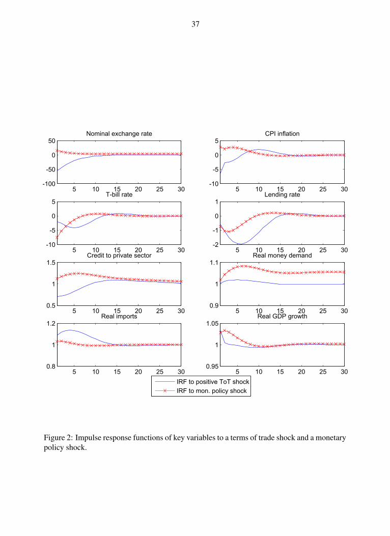
37

5 10 15 20 25 30-100

-50

0

50Nominal exchange rate

5 10 15 20 25 30-10

-5

0

5CPI inflation

5 10 15 20 25 30-10

-5

0

5T-bill rate

5 10 15 20 25 30-2

-1

0

1Lending rate

5 10 15 20 25 300.5

1

1.5Credit to private sector

5 10 15 20 25 300.9

1

1.1Real money demand

5 10 15 20 25 300.8

1

1.2Real imports

5 10 15 20 25 300.95

1

1.05Real GDP growth

IRF to positive ToT shock

IRF to mon. policy shock

Figure 2: Impulse response functions of key variables to a terms of trade shock and a monetarypolicy shock.

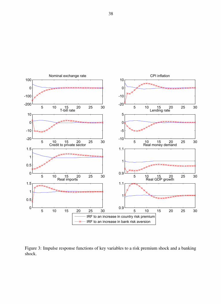
38

5 10 15 20 25 30-200

-100

0

100Nominal exchange rate

5 10 15 20 25 30-20

-10

0

10CPI inflation

5 10 15 20 25 30-20

-10

0

10T-bill rate

5 10 15 20 25 30-10

-5

0

5Lending rate

5 10 15 20 25 300

0.5

1

1.5Credit to private sector

5 10 15 20 25 300.9

1

1.1Real money demand

5 10 15 20 25 300

0.5

1

1.5Real imports

5 10 15 20 25 300.9

1

1.1Real GDP growth

IRF to an increase in country risk premium

IRF to an increase in bank risk aversion

Figure 3: Impulse response functions of key variables to a risk premium shock and a bankingshock.

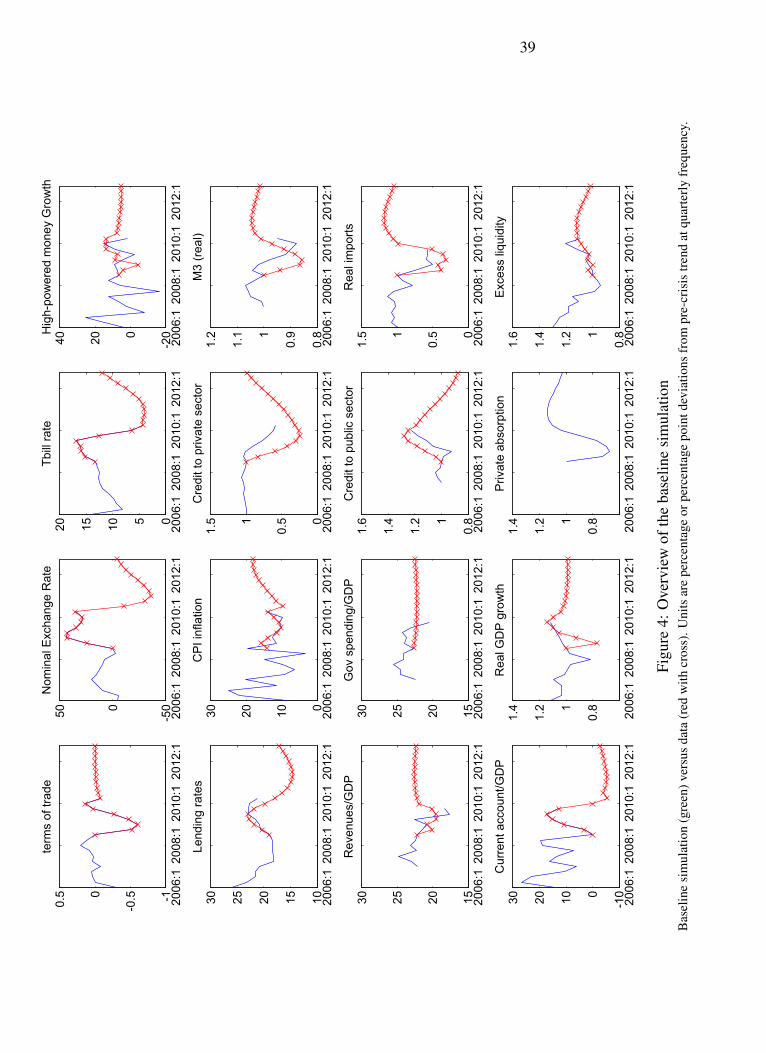
39

2006

:120

08:1

2010

:120

12:1

-1

-0.50

0.5

term

s of

trad

e

2006

:120

08:1

2010

:120

12:1

-50050

Nom

inal

Exc

hang

e R

ate

2006

:120

08:1

2010

:120

12:1

05101520T

bill

rate

2006

:120

08:1

2010

:120

12:1

-2002040H

igh-

pow

ered

mon

ey G

row

th

2006

:120

08:1

2010

:120

12:1

1015202530Le

ndin

g ra

tes

2006

:120

08:1

2010

:120

12:1

0102030C

PI i

nfla

tion

2006

:120

08:1

2010

:120

12:1

0

0.51

1.5

Cre

dit t

o pr

ivat

e se

ctor

2006

:120

08:1

2010

:120

12:1

0.8

0.91

1.1

1.2

M3

(rea

l)

2006

:120

08:1

2010

:120

12:1

15202530R

even

ues/

GD

P

2006

:120

08:1

2010

:120

12:1

15202530G

ov s

pend

ing/

GD

P

2006

:120

08:1

2010

:120

12:1

0.81

1.2

1.4

1.6

Cre

dit t

o pu

blic

sec

tor

2006

:120

08:1

2010

:120

12:1

0

0.51

1.5

Rea

l im

port

s

2006

:120

08:1

2010

:120

12:1

-100102030

Cur

rent

acc

ount

/GD

P

2006

:120

08:1

2010

:120

12:1

0.81

1.2

1.4

Rea

l GD

P g

row

th

2006

:120

08:1

2010

:120

12:1

0.81

1.2

1.4

Priv

ate

abso

rptio

n

2006

:120

08:1

2010

:120

12:1

0.81

1.2

1.4

1.6

Exc

ess

liqui

dity

Figu

re4:

Ove

rvie

wof

the

base

line

sim

ulat

ion

Bas

elin

esi

mul

atio

n(g

reen

)ver

sus

data

(red

with

cros

s).U

nits

are

perc

enta

geor

perc

enta

gepo

intd

evia

tions

from

pre-

cris

istr

end

atqu

arte

rly

freq

uenc

y.

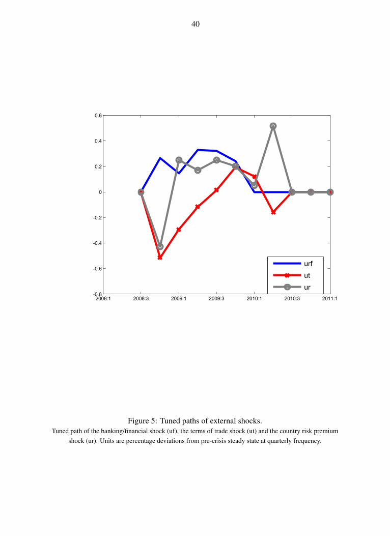
40

2008:1 2008:3 2009:1 2009:3 2010:1 2010:3 2011:1-0.8

-0.6

-0.4

-0.2

0

0.2

0.4

0.6

urf

ut

ur

Figure 5: Tuned paths of external shocks.Tuned path of the banking/financial shock (uf), the terms of trade shock (ut) and the country risk premium

shock (ur). Units are percentage deviations from pre-crisis steady state at quarterly frequency.

41

2008

:420

09:2

2009

:420

10:2

2010

:420

11:2

2011

:420

12:2

2012

:4

-200

-1000

100

200

300

uf ut ur um

2008

:420

09:2

2009

:420

10:2

2010

:420

11:2

2011

:420

12:2

-30

-20

-10010203040

Nom

inal

exc

hang

e ra

te

2008

:420

09:2

2009

:420

10:2

2010

:420

11:2

2011

:420

12:2

2012

:4-1

5

-10-5051015

uf ur ut um

2008

:420

09:2

2009

:420

10:2

2010

:420

11:2

2011

:420

12:2

-4-3-2-10123

Len

ding

rat

e

200

8:4

200

9:2

200

9:4

201

0:2

201

0:4

201

1:2

201

1:4

201

2:2

201

2:4

-30

-20

-100

10

20

30

40

uf

ur

ut

um

200

8:4

200

9:2

200

9:4

201

0:2

201

0:4

201

1:2

201

1:4

201

2:2

-4-3-2-10123

Infl

ati

on

Figu

re6:

Stru

ctur

alsh

ock

deco

mpo

sitio

n1.

Bas

elin

esi

mul

atio

npa

ths

fors

elec

ted

pric

eva

riab

les

and

thei

rdec

ompo

sitio

nto

4st

ruct

ural

shoc

ksof

the

mod

el.U

nits

are

perc

enta

gepo

intd

evia

tions

from

pre-

cris

istr

end

atqu

arte

rly

freq

uenc

y.

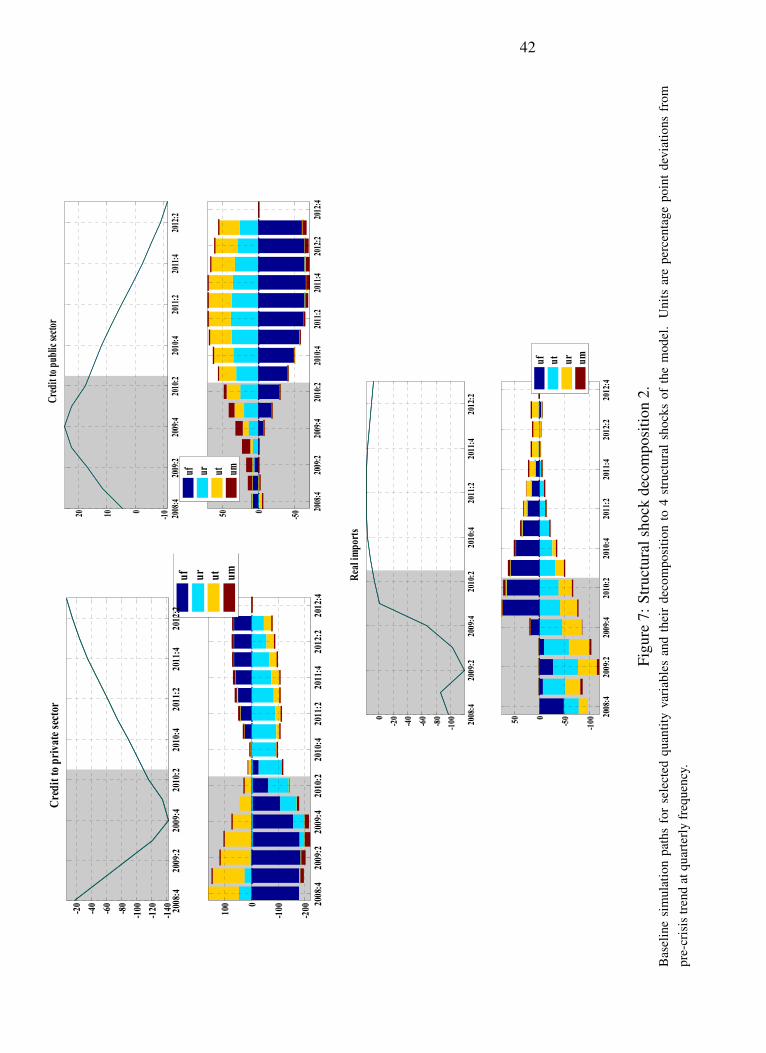
42

2008

:420

09:2

2009

:420

10:2

2010

:420

11:2

2011

:420

12:2

2012

:4-2

00

-1000

100

uf ur ut um

2008

:420

09:2

2009

:420

10:2

2010

:420

11:2

2011

:420

12:2

-140

-120

-100-8

0

-60

-40

-20

Cre

dit t

o pr

ivat

e se

ctor

2008

:420

09:2

2009

:420

10:2

2010

:420

11:2

2011

:420

12:2

2012

:4

-50050

uf ur ut um

2008

:420

09:2

2009

:420

10:2

2010

:420

11:2

2011

:420

12:2

-1001020

Cred

it to

pub

lic se

ctor

2008

:420

09:2

2009

:420

10:2

2010

:420

11:2

2011

:420

12:2

2012

:4

-100-5

0050

uf ut ur um

2008

:420

09:2

2009

:420

10:2

2010

:420

11:2

2011

:420

12:2

-100-8

0

-60

-40

-200

Rea

l im

port

s

Figu

re7:

Stru

ctur

alsh

ock

deco

mpo

sitio

n2.

Bas

elin

esi

mul

atio

npa

ths

for

sele

cted

quan

tity

vari

able

san

dth

eir

deco

mpo

sitio

nto

4st

ruct

ural

shoc

ksof

the

mod

el.

Uni

tsar

epe

rcen

tage

poin

tde

viat

ions

from

pre-

cris

istr

end

atqu

arte

rly

freq

uenc

y.

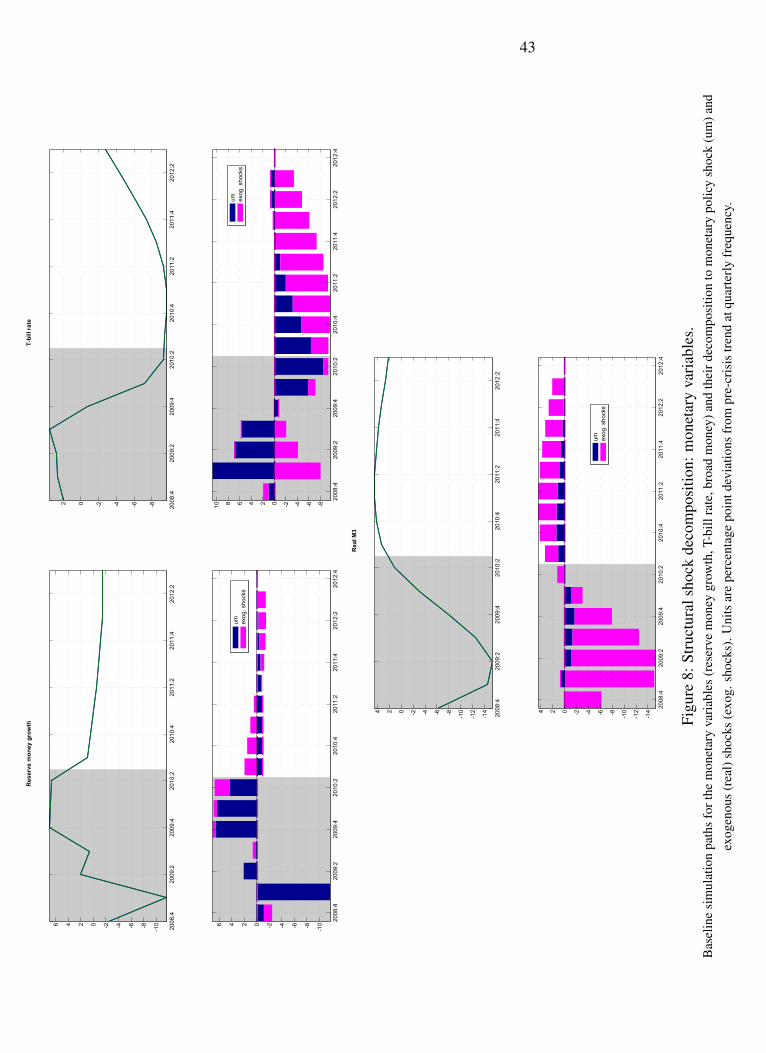
43

2008

:420

09:2

2009

:420

10:2

2010

:420

11:2

2011

:420

12:2

2012

:4

-10-8-6-4-20246

um exog

. sho

cks

2008

:420

09:2

2009

:420

10:2

2010

:420

11:2

2011

:420

12:2

-10-8-6-4-20246

Res

erve

mon

ey g

row

th

2008

:420

09:2

2009

:420

10:2

2010

:420

11:2

2011

:420

12:2

2012

:4

-8-6-4-20246810

um exog

. sho

cks

2008

:420

09:2

2009

:420

10:2

2010

:420

11:2

2011

:420

12:2

-8-6-4-202

T-bi

ll ra

te

2008

:420

09:2

2009

:420

10:2

2010

:420

11:2

2011

:420

12:2

2012

:4

-14

-12

-10-8-6-4-2024

um exog

. sho

cks

2008

:420

09:2

2009

:420

10:2

2010

:420

11:2

2011

:420

12:2

-14

-12

-10-8-6-4-2024

Rea

l M3

Figu

re8:

Stru

ctur

alsh

ock

deco

mpo

sitio

n:m

onet

ary

vari

able

s.B

asel

ine

sim

ulat

ion

path

sfo

rthe

mon

etar

yva

riab

les

(res

erve

mon

eygr

owth

,T-b

illra

te,b

road

mon

ey)a

ndth

eird

ecom

posi

tion

tom

onet

ary

polic

ysh

ock

(um

)and

exog

enou

s(r

eal)

shoc

ks(e

xog.

shoc

ks).

Uni

tsar

epe

rcen

tage

poin

tdev

iatio

nsfr

ompr

e-cr

isis

tren

dat

quar

terl

yfr

eque

ncy.

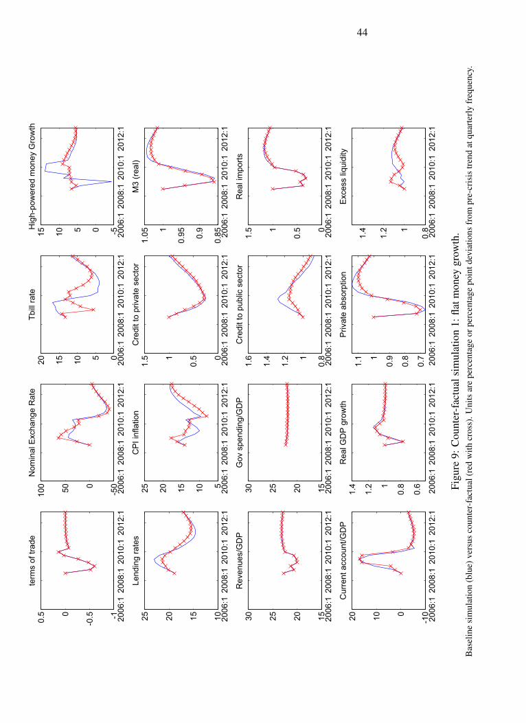
44

2006

:120

08:1

2010

:120

12:1

-1

-0.50

0.5

term

s of

trad

e

2006

:120

08:1

2010

:120

12:1

-50050100

Nom

inal

Exc

hang

e R

ate

2006

:120

08:1

2010

:120

12:1

05101520T

bill

rate

2006

:120

08:1

2010

:120

12:1

-5051015H

igh-

pow

ered

mon

ey G

row

th

2006

:120

08:1

2010

:120

12:1

10152025Le

ndin

g ra

tes

2006

:120

08:1

2010

:120

12:1

510152025C

PI i

nfla

tion

2006

:120

08:1

2010

:120

12:1

0

0.51

1.5

Cre

dit t

o pr

ivat

e se

ctor

2006

:120

08:1

2010

:120

12:1

0.850.9

0.951

1.05

M3

(rea

l)

2006

:120

08:1

2010

:120

12:1

15202530R

even

ues/

GD

P

2006

:120

08:1

2010

:120

12:1

15202530G

ov s

pend

ing/

GD

P

2006

:120

08:1

2010

:120

12:1

0.81

1.2

1.4

1.6

Cre

dit t

o pu

blic

sec

tor

2006

:120

08:1

2010

:120

12:1

0

0.51

1.5

Rea

l im

port

s

2006

:120

08:1

2010

:120

12:1

-1001020

Cur

rent

acc

ount

/GD

P

2006

:120

08:1

2010

:120

12:1

0.6

0.81

1.2

1.4

Rea

l GD

P g

row

th

2006

:120

08:1

2010

:120

12:1

0.7

0.8

0.91

1.1

Priv

ate

abso

rptio

n

2006

:120

08:1

2010

:120

12:1

0.81

1.2

1.4

Exc

ess

liqui

dity

Figu

re9:

Cou

nter

-fac

tual

sim

ulat

ion

1:fla

tmon

eygr

owth

.B

asel

ine

sim

ulat

ion

(blu

e)ve

rsus

coun

ter-

fact

ual(

red

with

cros

s).U

nits

are

perc

enta

geor

perc

enta

gepo

intd

evia

tions

from

pre-

cris

istr

end

atqu

arte

rly

freq

uenc

y.

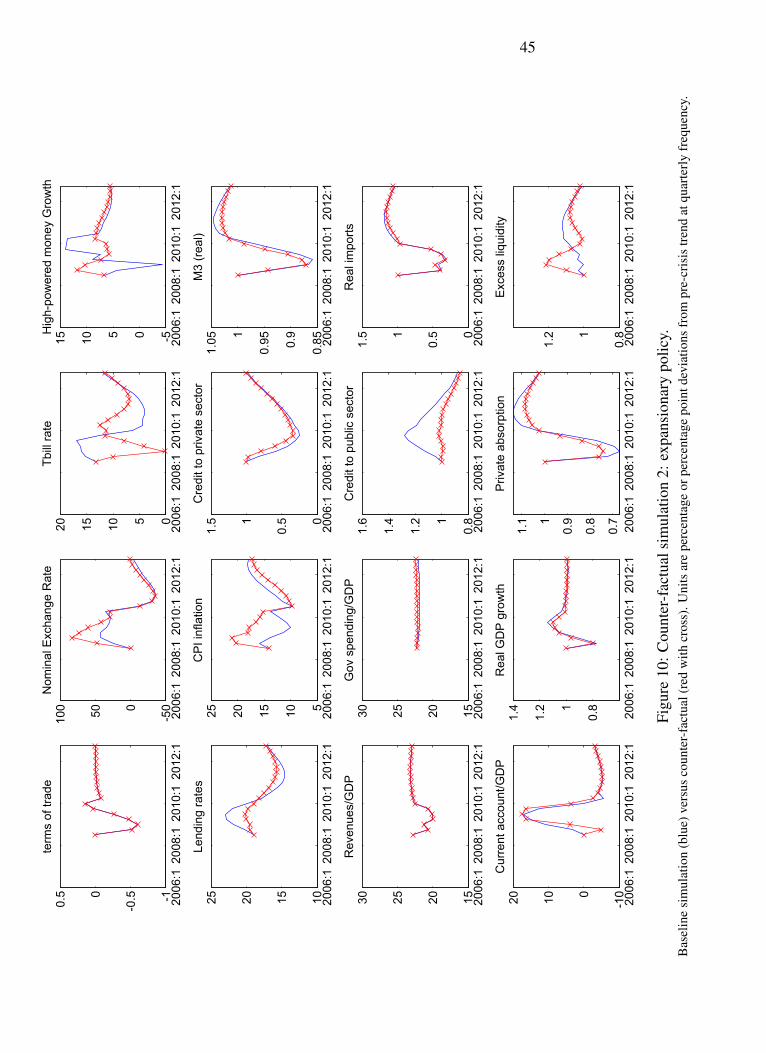
45

2006

:120

08:1

2010

:120

12:1

-1

-0.50

0.5

term

s of

trad

e

2006

:120

08:1

2010

:120

12:1

-50050100

Nom

inal

Exc

hang

e R

ate

2006

:120

08:1

2010

:120

12:1

05101520T

bill

rate

2006

:120

08:1

2010

:120

12:1

-5051015H

igh-

pow

ered

mon

ey G

row

th

2006

:120

08:1

2010

:120

12:1

10152025Le

ndin

g ra

tes

2006

:120

08:1

2010

:120

12:1

510152025C

PI i

nfla

tion

2006

:120

08:1

2010

:120

12:1

0

0.51

1.5

Cre

dit t

o pr

ivat

e se

ctor

2006

:120

08:1

2010

:120

12:1

0.850.9

0.951

1.05

M3

(rea

l)

2006

:120

08:1

2010

:120

12:1

15202530R

even

ues/

GD

P

2006

:120

08:1

2010

:120

12:1

15202530G

ov s

pend

ing/

GD

P

2006

:120

08:1

2010

:120

12:1

0.81

1.2

1.4

1.6

Cre

dit t

o pu

blic

sec

tor

2006

:120

08:1

2010

:120

12:1

0

0.51

1.5

Rea

l im

port

s

2006

:120

08:1

2010

:120

12:1

-1001020

Cur

rent

acc

ount

/GD

P

2006

:120

08:1

2010

:120

12:1

0.81

1.2

1.4

Rea

l GD

P g

row

th

2006

:120

08:1

2010

:120

12:1

0.7

0.8

0.91

1.1

Priv

ate

abso

rptio

n

2006

:120

08:1

2010

:120

12:1

0.81

1.2

Exc

ess

liqui

dity

Figu

re10

:Cou

nter

-fac

tual

sim

ulat

ion

2:ex

pans

iona

rypo

licy.

Bas

elin

esi

mul

atio

n(b

lue)

vers

usco

unte

r-fa

ctua

l(re

dw

ithcr

oss)

.Uni

tsar

epe

rcen

tage

orpe

rcen

tage

poin

tdev

iatio

nsfr

ompr

e-cr

isis

tren

dat

quar

terl

yfr

eque

ncy.

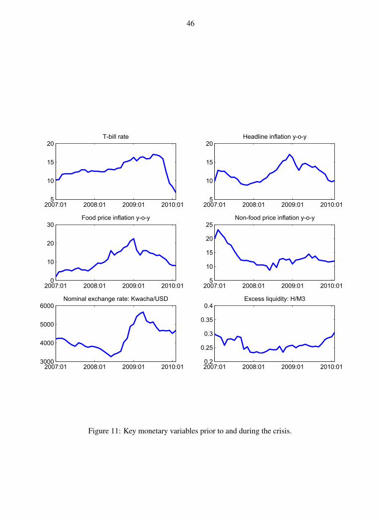
46

2007:01 2008:01 2009:01 2010:015

10

15

20T-bill rate

2007:01 2008:01 2009:01 2010:015

10

15

20Headline inflation y-o-y

2007:01 2008:01 2009:01 2010:010

10

20

30Food price inflation y-o-y

2007:01 2008:01 2009:01 2010:015

10

15

20

25Non-food price inflation y-o-y

2007:01 2008:01 2009:01 2010:013000

4000

5000

6000Nominal exchange rate: Kwacha/USD

2007:01 2008:01 2009:01 2010:010.2

0.25

0.3

0.35

0.4Excess liquidity: H/M3

Figure 11: Key monetary variables prior to and during the crisis.