Embed Size (px)
Citation preview
Bank of Canada staff working papers provide a forum for staff to publish work‐in‐progress research independently from the Bank’s Governing
Council. This research may support or challenge prevailing policy orthodoxy. Therefore, the views expressed in this paper are solely those of the authors and may differ from official Bank of Canada views. No responsibility for them should be attributed to the Bank.
www.bank‐banque‐canada.ca
Staff Working Paper/Document de travail du personnel 2017‐25
Monetary Policy Implementation in a Negative Rate Environment
by Michael Boutros and Jonathan Witmer
2
Bank of Canada Staff Working Paper 2017-25
July 2017
Monetary Policy Implementation in a Negative Rate Environment
by
Michael Boutros1 and Jonathan Witmer2
1Duke University [email protected]
2Financial Markets Department
Bank of Canada Ottawa, Ontario, Canada K1A 0G9
ISSN 1701-9397 © 2017 Bank of Canada

i
Acknowledgements
We thank Greg Bauer, David Cimon, Corey Garriott, Chris Sutherland, Jing Yang and seminar participants at the Bank of Canada for their helpful comments. All remaining errors are our own.

ii
Abstract Monetary policy implementation could, in theory, be constrained by deeply negative rates since overnight market participants may have an incentive to invest in cash rather than lend to other participants. To understand the functioning of overnight markets in such an environment, we add the option to exchange central bank reserves for cash to the standard workhorse model of monetary policy implementation (Poole 1968). Importantly, we show that monetary policy is not constrained when just the deposit rate is below the yield on cash. However, it could be constrained when the target overnight rate is below the yield on cash. At this point, the overnight rate equals the yield on cash instead of the target rate. Modifications to the implementation framework, such as a tiered remuneration of central bank deposits contingent on cash withdrawals, can work to restore the implementation of monetary policy such that the overnight rate equals the target rate.
Bank topics: Interest rates; Monetary policy implementation; Monetary policy framework JEL codes: E4, E40, E42, E43, G, G0
Résumé Des taux d’intérêt fortement négatifs pourraient, en théorie, faire peser une contrainte sur la mise en œuvre de la politique monétaire, puisque les participants aux marchés du financement à un jour pourraient dans ce cas avoir avantage à transformer leurs fonds en espèces plutôt qu’à les prêter aux autres participants. Pour appréhender le fonctionnement des marchés du financement à un jour dans ce contexte, nous intégrons la possibilité d’échanger des réserves à la banque centrale contre des espèces dans le principal modèle de mise en œuvre de la politique monétaire (Poole, 1968). Plus particulièrement, nous montrons qu’il ne suffit pas que le taux de rémunération des dépôts se situe en deçà du rendement obtenu par la détention d’espèces pour que s’exerce une contrainte sur la politique monétaire. La politique monétaire peut en revanche être limitée dans son action lorsque le taux cible du financement à un jour est inférieur au rendement dégagé par les espèces. Le taux du financement sur le marché à un jour est alors égal au rendement des espèces et non plus au taux cible. Des modifications apportées au cadre de conduite de la politique monétaire, telle une rémunération par segment des dépôts à la banque centrale qui serait fonction des retraits d’espèces effectués, peuvent aider à rétablir l’égalité entre le taux sur le marché à un jour et le taux cible.
Sujets : Taux d’intérêt ; Mise en œuvre de la politique monétaire ; Cadre de la politique monétaire Codes JEL : E4, E40, E42, E43, G, G0
Non‐Technical Summary
The transmission of negative policy interest rates to longer‐term market interest rates depends first on
the ability of central banks to steer the overnight rate towards the desired target rate. Most central
banks operate by setting a target for the overnight interest rate, along with rates on standing facilities
through which participants can borrow from or deposit with the central bank. This creates incentives for
overnight market participants to trade with each other within the band created by the central bank
borrowing and deposit rates. When the rates on these standing facilities become negative enough,
overnight market participants may have an incentive to invest in cash rather than lend to other
participants in the overnight market. This could, in theory, have an effect on the ability of the central
bank to implement monetary policy.
To understand the functioning of overnight markets in such an environment, we account for the
effective lower bound by adding the option to exchange central bank reserves for cash to the standard
workhorse model of monetary policy implementation. The model shows that, when the target for the
policy rate is below the nominal return on cash, participants have an incentive to convert reserves to
cash rather than lend to other participants. Because of this, they may remove reserves from the system,
which puts upward pressure on the overnight rate. In equilibrium, reserves will be removed such that
the overnight rate will equal the return on cash.
Some central banks have moved to a tiered remuneration of deposits in a negative interest rate
environment. In this framework, deposits with the central bank up to a certain threshold are
remunerated at a higher rate, typically zero basis points. Deposits above this threshold are remunerated
at a negative rate (i.e., participants pay to have deposits with the central bank). This threshold is
lowered if participants convert reserves to cash. We show how these modifications within our model
can change incentives and limit the impact of negative interest rates on the overnight interest rate. Our
model shows that it is not the tiered remuneration in and of itself that changes incentives to withdraw
from the central bank; rather, it is the fact that this tiered remuneration is a function of cash
withdrawals that can disincentivize these withdrawals such that the overnight rate once again equals
the target rate.
We also consider a model with reserve requirements that are a function of cash withdrawals. Within our
model framework, a varying reserve requirement is more powerful than a varying tiered remuneration
in disincentivizing cash withdrawals. This stronger disincentive occurs because, with some probability,
banks may not be fully utilizing their exemption threshold in a tiered remuneration framework, so a
change in this exemption threshold has a less powerful effect on their incentives.
1 Introduction
Central banks have significantly altered their monetary policy implementation
frameworks in the aftermath of the financial crisis. First, quantitative easing
resulted in an increase in central bank reserves, which significantly changed
trading incentives and behavior in the market for overnight reserves. In 2008, the
Federal Reserve introduced interest on reserves as a way to maintain influence
over the overnight rate because of a significant increase in reserves (Klee et al.
(2016)). More recently, several central banks including the European Central
Bank (ECB), the Swiss National Bank (SNB) and the Bank of Japan (BoJ)
have adopted negative policy rates.
Central banks implement monetary policy differently, and it is not appar-
ent how differences in monetary policy implementation frameworks matter in a
negative rate environment. Most central banks operate by setting a target for
the overnight interest rate, along with rates on standing facilities through which
participants can borrow from or deposit with the central bank (Borio, 1997).
Some central banks, like the Bank of Canada, operate a corridor system whereby
the target rate is in the middle of a corridor bounded by the (higher) borrowing
rate and the (lower) deposit rate (Bank of Canada, 2015). Others operate a
floor system – so named because the target rate is equal to the deposit rate at
the bottom of the interest rate corridor. Some central banks have even adapted
their frameworks as they lowered their policy rates into negative territory. The
Swiss National Bank, for instance, has transitioned to a tiered system for the
remuneration of deposits with the Swiss National Bank (Swiss National Bank,
2014). An amount of deposits with the Swiss National Bank is exempt from the
negative deposit rate and is compensated at a rate of zero. Any deposits above
this amount are compensated at a negative rate, meaning banks pay the Swiss
National Bank for these deposits. How were these changes important for the
implementation of monetary policy in a negative rate environment?
Monetary policy implementation is concerned with how short-term (usually
2
overnight) interest rates are determined and is the starting point of the monetary
policy transmission mechanism. Understanding the impact of negative rates on
monetary policy implementation is of practical importance since negative inter-
est rates are becoming more common. Over USD 13 trillion of sovereign bonds
has now traded at negative rates (Whittall and Goldfarb, 2016). And sovereign
bond yields in some countries are negative beyond ten years of maturity, sug-
gesting that negative rates are not expected to be a passing phenomenom.
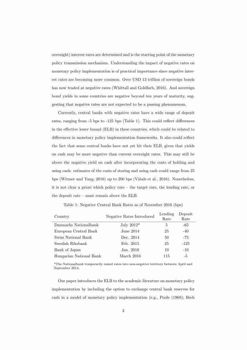
Currently, central banks with negative rates have a wide range of deposit
rates, ranging from -5 bps to -125 bps (Table 1). This could reflect differences
in the effective lower bound (ELB) in these countries, which could be related to
differences in monetary policy implementation frameworks. It also could reflect
the fact that some central banks have not yet hit their ELB, given that yields
on cash may be more negative than current overnight rates. This may still be
above the negative yield on cash after incorporating the costs of holding and
using cash: estimates of the costs of storing and using cash could range from 25
bps (Witmer and Yang, 2016) up to 200 bps (Vinals et al., 2016). Nonetheless,
it is not clear a priori which policy rate – the target rate, the lending rate, or
the deposit rate – must remain above the ELB.
Table 1: Negative Central Bank Rates as of November 2016 (bps)
Country Negative Rates IntroducedLending
RateDeposit
Rate
Danmarks Nationalbank July 2012* 5 -65
European Central Bank June 2014 25 -40
Swiss National Bank Dec. 2014 50 -75
Swedish Riksbank Feb. 2015 25 -125
Bank of Japan Jan. 2016 10 -10
Hungarian National Bank March 2016 115 -5
*The Nationalbank temporarily raised rates into non-negative territory between April andSeptember 2014.
Our paper introduces the ELB to the academic literature on monetary policy
implementation by including the option to exchange central bank reserves for
cash in a model of monetary policy implementation (e.g., Poole (1968); Bech
3
and Keister (2013)). The opportunity to invest in cash implies an effective lower
bound or constraint on overnight interest rates (e.g., Witmer and Yang (2016)),
and thus presents a potential obstacle to the implementation of monetary policy.
To the best of our knowledge, no other model has considered how the zero lower
bound and negative interest rates can impact monetary policy implementation.
Our model contributes several new insights to this literature. First, it is
the central bank target rate that must be above the ELB, not the central bank
deposit rate. Intuition would suggest that the deposit rate must be above the
ELB (i.e., the yield on the outside cash option), since participants would prefer
investing in cash over depositing at the central bank. However, they do not have
the ability to exchange cash for reserves at the end of the day after the uncertain
payment shock. The marginal cost of borrowing an extra dollar in the overnight
market – the overnight rate – is equal to the respective probabilities of accessing
the two central bank standing facilities at the end of the day multiplied by their
respective rates (Bindseil, 2001), with these probabilities determined by the
uncertainty inherent in the payment shock and the participant’s position just
prior to the shock. Thus, the yield on cash does not impact the overnight rate
as long as the target for the overnight rate is above the ELB. Put another way,
a participant with excess funds during the day would be better off lending to
participants at the target rate, rather than deposit in cash earning the cash yield,
as long as the target rate is above the return on cash. Similarly, participants
short of funds would not want to become even more short by investing in cash
since they would have to borrow even more from other participants at the higher
target rate.
Second, if the yield on cash is above the overnight target rate but below
the central bank lending rate, the overnight interest rate will equal the yield on
cash.1 Intuitively, participants would prefer to withdraw and invest in higher-
1When the yield on cash is above the central bank lending rate, participants would wantto borrow from the central bank and invest in cash, and there is no overnight market. Partic-ipants would not want to lend their funds below a rate they receive on investing in cash, andparticipants would not want to borrow funds above the rate they could attain when borrowingfrom the central bank.
4
yielding cash rather than lend to other participants at the target rate. Their
cash withdrawals will lower the overall amount of reserves in the system. In
equilibrium, the amount of reserves will adjust until the overnight rate is equal
to the return on cash.
Third, our model is the first to examine monetary policy implementation
with a tiered deposit rate that allows the tier thresholds to adjust depending
on the cash withdrawals of each participant. The Whitesell (2006) model shows
the conditions under which static tiered rates can be used to steer the overnight
rate towards the target overnight rate in a positive rate environment.2 Our
model shows how to extend this model to a negative interest rate environment
by adding the option to exchange reserves for cash. As well, we also allow
the tiered thresholds to vary with cash withdrawals, and demonstrate why this
feature is important for divorcing the overnight rate from the yield on cash. The
Bank of Japan and the European Central Bank, for example, have implemented
a tiered remuneration of central bank deposits. Our model shows that it is not
the tiered remuneration in and of itself that changes incentives to withdraw
from the central bank; rather, it is the fact that this tiered remuneration is a
function of cash withdrawals that can disincentivize these withdrawals such that
the overnight rate once again equals the target rate.
Finally, we develop a model with reserve requirements that are a function of
cash withdrawals. This has not been considered in the literature and has not
been implemented by any central bank in the negative rate environment. Within
our model framework, we show that a varying reserve requirement is more pow-
erful than a varying tiered remuneration in disincentivizing cash withdrawals.
This stronger disincentive occurs because, with some probability, banks may
not be fully utilizing their exemption threshold in a tiered remuneration frame-
work, so a change in this exemption threshold has a less powerful effect on their
2Different methods have been proposed and utilized for determining the size of the thresh-old. Whitesell (2006) suggests that the central bank could set the price of the thresholdamount and sell this threshold amount for a fee (e.g., 5 bps of the total size of the quota).Holthausen et al. (2008) propose that the central bank could set the quantity of the thresh-old, and either determine these limits in the same way as they currently determine reserverequirements, or auction the limits to participants.
5
incentives. Thus, according to our model, a varying reserve requirement will
better help a central bank maintain its influence over the overnight rate when
rates are potentially constrained by the lower bound.
Our paper is related to the literature that examines the impact of frictions
on monetary policy implementation since the ELB is a friction that can impact
the ability of a central bank to influence the overnight interest rate towards
its policy rate. Several papers consider how regulation, and in particular the
liquidity regulation of banks, will affect monetary policy implementation and
the functioning of money markets (Bech and Keister (2013), Banerjee and Mio
(2014), Bonner and Eijffinger (2012), Rezende et al. (2016)). Others examine
the effect of search frictions, which can generate predictions about volumes
and volatility of overnight rates (Bech and Monnet, Afonso and Lagos (2015),
Armenter and Lester (2015)). Another related set of papers also considers how
segmentation in the overnight market and differential access to central bank
facilities can have an impact on monetary policy implementation (Williamson
(2015), Bech and Klee (2011), Armenter and Lester (2015), Martin et al. (2013)).
Several of these papers show how the introduction of new tools, such as the
Federal Reserve’s overnight reverse repurchase facility (ORRP) and term deposit
facility (TDF) can work to attenuate the effects due to segmentation. Similarly,
we show how alterations to the monetary policy implementation framework can
attenuate the impact of the ELB on overnight interest rates.
Since we are examining the ELB, our paper also complements the strand
of the literature that analyzes the effect of unconventional tools such as quan-
titative easing and the resulting large central bank balance sheets and excess
reserves on the determination of the overnight interest rate. Kashyap and Stein
(2012), for instance, point out that when the central bank has large excess re-
serves it essentially has two tools: the interest it pays on reserves, as well as
the quantity of those reserves. They suggest that the central bank then has
the capability of pursuing two objectives: an inflation objective, and an objec-
tive to reduce the externalities created by excessive short-term debt issuance
6
by financial intermediaries. Some recent papers discuss how these tools can be
used in the exit from unconventional monetary policy (Bech and Klee (2011),
Armenter and Lester (2015), Ihrig et al. (2015)). The ELB may limit the ability
of the central bank to adjust one of these tools (the interest on reserves), and
our model examines how adjustments to implementation frameworks may work
to restore this ability.
Given this, it also relates to recent papers that suggest how the ELB could be
lowered or removed. If the central bank restricts conversions of reserves to cash
or increases the aggregate stock of paper currency according to a pre-defined
rule, a market-determined deposit price of paper currency may develop even if
the central bank is still exchanging reserves for cash at par (Goodfriend, 2016).
Goodfriend argues that this could, in theory, help to overcome the lower bound
on interest rates. However, it may also require changes such that contracts
are enforced to be paid in deposits rather than paper currency (Agarwal and
Kimball, 2015). Similarly, the central bank could charge a time-varying paper
currency deposit fee to eliminate the incentive to withdraw cash to avoid neg-
ative interest rates (Agarwal and Kimball, 2015). In our model, an adjustable
system of tiered remuneration can also reduce this incentive to withdraw cash.
It shows how such an adjustable tiered remuneration could be used to reduce
the friction associated with the lower bound, at least to a certain degree.
In the next section, we provide the details of our basic model before examin-
ing equilibrium impacts in section 3. Section 4 provides a numerical example to
illustrate how the model would work in practice. We consider modifications to
our basic model in section 5. In particular, we focus on how a tiered remunera-
tion of central bank reserves (such as is implemented by the Bank of Japan) can
work to mitigate the impact of the ELB on the overnight market. We conclude
with a short discusion in section 6.
7
2 The Model
We employ a static model similar to the one in Bech and Keister (2013). Per-
fectly competitive banks are profit maximizers that must respect a reserve re-
quirement determined by the central bank, which could in fact be zero.
A bank begins the day by observing its own holdings of liabilities and assets,
including the amount of reserves it holds and its reserve requirement. Next, the
bank can increase (decrease) reserves by borrowing (lending) on the interbank
market or can decrease reserves by converting them to cash. The bank faces
uncertainty with regards to the optimal amount of interbank borrowing and
lending because after the interbank market closes, the bank uses its reserves to
continue allowing deposits and withdrawals from customers.
At the end of the day, the bank determines if the new level of reserves
meets the reserve requirement set by the central bank. If its reserves are lower
than its reserve requirement at the end of the day, the bank borrows directly
from the central bank at a rate of rX . Likewise, any reserves in excess of the
requirement are deposited with the central bank at the end of the day at a return
on excess reserves rate rR. Poole (1968) shows (under reasonable assumptions)
that borrowing from the central bank is essentially always more expensive than
borrowing on the interbank market.
The model’s timing is similar to other models of monetary policy implemen-
tation, with the exception that it includes an opportunity to exchange reserves
for cash during the day. Our results depend on the timing of the reserve-cash
conversion. For example, if commercial banks could exchange reserves for cash
after their deposit shocks are realized, the equilibrium interbank rate would be
very different. In essence, if the return on cash was greater than the central bank
deposit rate, commercial banks would not use the deposit facility and would in-
stead earn the return on cash. The equilibrium rate would then be determined
by the return on cash and the central bank borrowing rate, the same way it is
determined by the central bank deposit rate and borrowing rate in the standard
8
model of monetary policy implementation.
Assumption 1. The cost of borrowing from the central bank is always strictly
larger than the return on excess reserves: rX > rR.
If this were not the case, then commercial banks could exploit an arbitrage
opportunity by borrowing from the central bank at rX and earning rR on the
borrowed funds by storing them as excess reserves.
Assumption 2. The return on cash is strictly nonpositive: rC ≤ 0.
This assumption is not critical for the model’s results. It is made to analyze
the effects of negative interest rates on monetary policy implementation. If the
nominal return on cash was positive, monetary policy implementation may be
impacted when rates are positive. There is nothing inherently special about
negative rates. Instead, the underlying issue is that cash, which is generally
believed to have a zero nominal return, now yields a higher return than reserves.
Cash is substitutable for reserves because they both share the qualities of zero
default risk and easy access. For the most part, people believe the nominal
return on cash to be exactly zero, but in reality the return on cash is slightly
negative because of the costs of storing and insuring cash holdings. Recent work
has estimated the return on cash to be somewhere around −0.5% (Witmer and
Yang, 2016).
For our purposes, the exact levels of the two central bank rates and the
return on cash are irrelevant, as what matters is the relationship between them.
Both for simplicity and to keep the discussion relevant, we focus on the realistic
scenario where the return on cash is zero or slightly negative.
2.1 Banks
A continuum of banks indexed by i ∈ [0, 1] are identical and take market rates
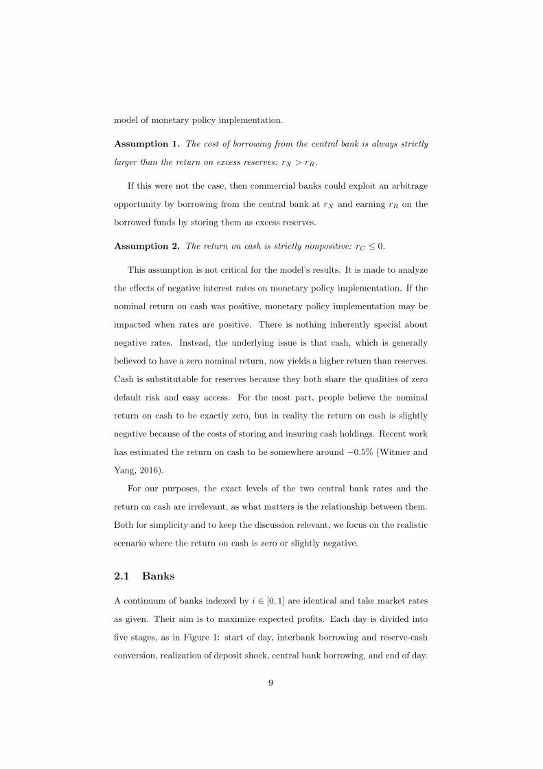
as given. Their aim is to maximize expected profits. Each day is divided into
five stages, as in Figure 1: start of day, interbank borrowing and reserve-cash
conversion, realization of deposit shock, central bank borrowing, and end of day.
9
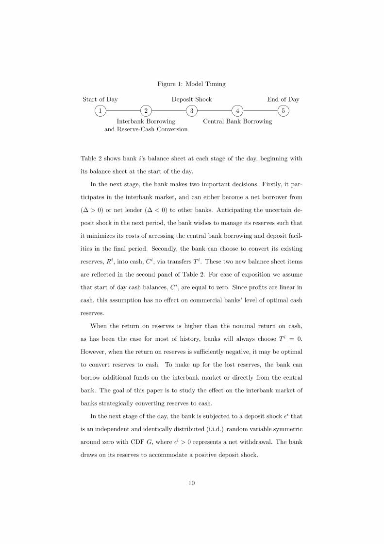
Figure 1: Model Timing
1 2 3 4 5
Start of Day
Interbank Borrowingand Reserve-Cash Conversion
Deposit Shock
Central Bank Borrowing
End of Day
Table 2 shows bank i’s balance sheet at each stage of the day, beginning with
its balance sheet at the start of the day.
In the next stage, the bank makes two important decisions. Firstly, it par-
ticipates in the interbank market, and can either become a net borrower from
(∆ > 0) or net lender (∆ < 0) to other banks. Anticipating the uncertain de-
posit shock in the next period, the bank wishes to manage its reserves such that
it minimizes its costs of accessing the central bank borrowing and deposit facil-
ities in the final period. Secondly, the bank can choose to convert its existing
reserves, Ri, into cash, Ci, via transfers T i. These two new balance sheet items
are reflected in the second panel of Table 2. For ease of exposition we assume
that start of day cash balances, Ci, are equal to zero. Since profits are linear in
cash, this assumption has no effect on commercial banks’ level of optimal cash
reserves.
When the return on reserves is higher than the nominal return on cash,
as has been the case for most of history, banks will always choose T i = 0.
However, when the return on reserves is sufficiently negative, it may be optimal
to convert reserves to cash. To make up for the lost reserves, the bank can
borrow additional funds on the interbank market or directly from the central
bank. The goal of this paper is to study the effect on the interbank market of
banks strategically converting reserves to cash.
In the next stage of the day, the bank is subjected to a deposit shock εi that
is an independent and identically distributed (i.i.d.) random variable symmetric
around zero with CDF G, where εi > 0 represents a net withdrawal. The bank
draws on its reserves to accommodate a positive deposit shock.
10
Table 2: Commercial Bank i’s Balance Sheet
Assets Liabilities
Stage 1: Start of Day
Bi Bonds Di Deposits
Ci Cash Ei Equity
Ri Reserves
Stage 2: Interbank Borrowing and Reserve-Cash Conversion
Bi Bonds Di Deposits
Ci + T i Cash Ei Equity
Ri + ∆i − T i Reserves ∆i Interbank Borrowing
Stage 3: Deposit Shock
Bi Bonds Di − εi Deposits
Ci + T i Cash Ei Equity
Ri + ∆i − T i − εi Reserves ∆i Interbank Borrowing
Stage 4 and 5: Central Bank Borrowing (End of Day)
Bi Bonds Di − εi Deposits
Ci + T i Cash Ei Equity
Ri + ∆i − T i − εi + Xi Reserves ∆i Interbank Borrowing
Xi Central Bank Borrowing
Notes: This table itemizes commercial bank i’s balance sheet at each stage of the day.Stages four (Central Bank Borrowing) and five (End of Day) are combined. In stage five,bank profits are realized.
Upon realization of ε, the bank may now hold less reserves than required.
If this is the case, in stage five the bank is forced to borrow from the central
bank to meet the reserve requirement. We impose the restriction that Xi ≥ 0 so
that the commercial bank cannot lend to the central bank at the central bank
lending rate. In the final stage of the day, the bank’s profits are realized.
Since most items appear identically on both sides of the balance sheet, each
bank’s balance sheet identity reduces to a simple expression:
Bi + Ci +Ri = Di + Ei (1)
11
2.2 Reserve Requirement
Each bank’s total end-of-day reserves must meet the bank’s individual reserve
requirement, Ki:
Ri +Xi + ∆i − T i − εi ≥ Ki (2)
Ki may be set to some constant for all banks, such as zero, constituting an
economy-wide reserve requirement. Alternatively, we leave open the possibility
that the central bank sets bank-specific conditional reserve requirements. Later,
we will show that bank-specific conditional reserve requirements can be used to
deter banks from converting reserves to cash in a negative rate environment.
Central bank borrowing Xi must be non-negative and is only utilized if
necessary; that is, if total reserves after the deposit shock are less than the
reserve requirement. Thus:
Xi = max{0,Ki − (Ri + ∆i − T i − εi)} (3)
Rearranging around the deposit shock, we can determine that central bank
borrowing only occurs if:
εi ≥ Ri + ∆i − T i −Ki ≡ εiK (4)
where εiK is excess reserves for bank i after the interbank market closes (and
before central bank borrowing occurs). This equation formalizes the intuition
developed earlier: if the deposit shock is greater than the bank’s excess reserves
following the interbank trading period, the bank will be forced to borrow from
the central bank at the end of the day. We can now more succinctly present
central bank borrowing as:
Xi = max{0, εi − εiK} (5)
12
2.3 Bank Profits
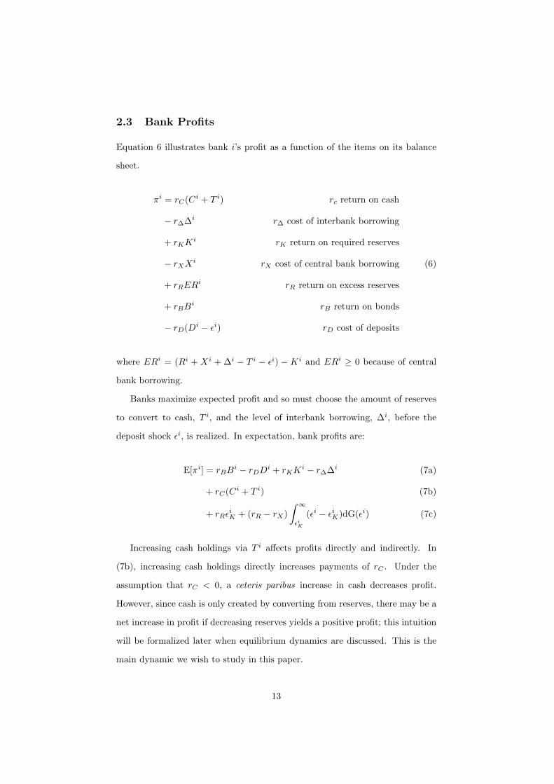
Equation 6 illustrates bank i’s profit as a function of the items on its balance
sheet.
πi = rC(Ci + T i) rc return on cash
− r∆∆i r∆ cost of interbank borrowing
+ rKKi rK return on required reserves
− rXXi rX cost of central bank borrowing (6)
+ rRERi rR return on excess reserves
+ rBBi rB return on bonds
− rD(Di − εi) rD cost of deposits
where ERi = (Ri + Xi + ∆i − T i − εi) −Ki and ERi ≥ 0 because of central
bank borrowing.
Banks maximize expected profit and so must choose the amount of reserves
to convert to cash, T i, and the level of interbank borrowing, ∆i, before the
deposit shock εi, is realized. In expectation, bank profits are:
E[πi] = rBBi − rDDi + rKK
i − r∆∆i (7a)
+ rC(Ci + T i) (7b)
+ rRεiK + (rR − rX)
∫ ∞εiK
(εi − εiK)dG(εi) (7c)
Increasing cash holdings via T i affects profits directly and indirectly. In
(7b), increasing cash holdings directly increases payments of rC . Under the
assumption that rC < 0, a ceteris paribus increase in cash decreases profit.
However, since cash is only created by converting from reserves, there may be a
net increase in profit if decreasing reserves yields a positive profit; this intuition
will be formalized later when equilibrium dynamics are discussed. This is the
main dynamic we wish to study in this paper.
13
The indirect effect of cash transfers manifests itself in (7c) twice. Firstly,
increasing cash decreases excess reserves and their associated returns before
central bank borrowing (εiK) . Secondly, decreasing excess reserves lowers the
threshold that triggers requiring a central bank loan; for a given deposit shock
εi, increasing cash increases the likelihood that borrowing from the central bank
at rate rX will be required. At the same time, funds borrowed from the central
bank are used as reserves and count towards the “excess reserves” level which
earns rR.
When the return on reserves is greater than the return on cash, increasing
cash by reducing excess reserves lowers profits, and T i = 0 is clearly the optimal
choice. When the return on reserves is less than the return on cash, however,
it may be optimal to convert some reserves to cash, but this has the additional
consequences discussed above.
The final term in (7c) is always negative because even though the deposit
shock is zero in expectation, a positive shock (i.e., εi > εiK , net withdrawal)
incurs a cost because banks must borrow from the central bank at rate rX ,
while they cannot profit from a negative shock (i.e., net deposit) by lending to
the central bank at the same rate (since Xi ≥ 0).3
Using interbank loans to hedge against central bank borrowing caused by a
positive deposit shock is the main equilibrium determinant of r∆. Thus, there
is a clear relationship between the interbank rate and both the cost of central
bank borrowing, rX , and the opportunity cost (to the lender) of an interbank
loan, rR.
Since a given deposit shock is more likely to induce central bank borrowing
for a lower level of reserves, and since more cash conversions implies lower
reserves, then, in an environment where non-zero reserve-to-cash conversions
are optimal, the level of cash conversions will also have a bearing on equilibrium
determination of the interbank rate.
3To see this more clearly, one can remove the restriction that Xi ≥ 0 and find that r∆ =rX , implying that banks borrow on the interbank market until the rate is exactly equal toborrowing directly from the central bank.
14
3 Equilibrium
In this section, we formalize the intuition described above into an equilib-
rium definition, and examine different outcomes under different monetary policy
regimes and central bank rates.
Definition. An equilibrium is a set of individual bank choices (∆i, T i, Xi) and
interest rate r∆ such that:
(i) Banks maximize expected profit, (7), subject to their balance sheet con-
straint, (1), and T i ≥ 0.
(ii) The interbank market is closed, that is, ∆ =
∫i
∆idi = 0.
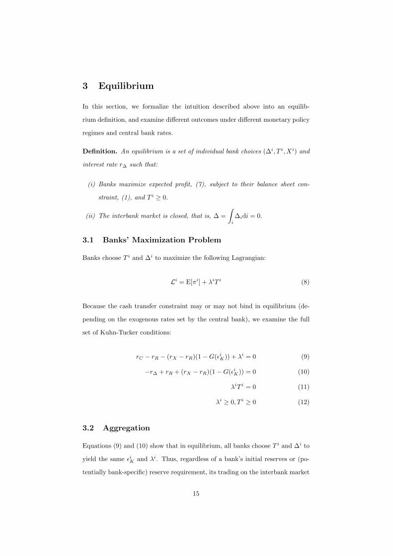
3.1 Banks’ Maximization Problem
Banks choose T i and ∆i to maximize the following Lagrangian:
Li = E[πi] + λiT i (8)
Because the cash transfer constraint may or may not bind in equilibrium (de-
pending on the exogenous rates set by the central bank), we examine the full
set of Kuhn-Tucker conditions:
rC − rR − (rX − rR)(1−G(εiK)) + λi = 0 (9)
−r∆ + rR + (rX − rR)(1−G(εiK)) = 0 (10)
λiT i = 0 (11)
λi ≥ 0, T i ≥ 0 (12)
3.2 Aggregation
Equations (9) and (10) show that in equilibrium, all banks choose T i and ∆i to
yield the same εiK and λi. Thus, regardless of a bank’s initial reserves or (po-
tentially bank-specific) reserve requirement, its trading on the interbank market
15
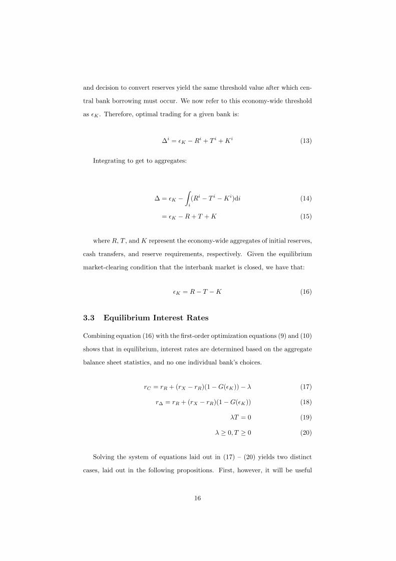
and decision to convert reserves yield the same threshold value after which cen-
tral bank borrowing must occur. We now refer to this economy-wide threshold
as εK . Therefore, optimal trading for a given bank is:
∆i = εK −Ri + T i +Ki (13)
Integrating to get to aggregates:
∆ = εK −∫i
(Ri − T i −Ki)di (14)
= εK −R+ T +K (15)
where R, T , and K represent the economy-wide aggregates of initial reserves,
cash transfers, and reserve requirements, respectively. Given the equilibrium
market-clearing condition that the interbank market is closed, we have that:
εK = R− T −K (16)
3.3 Equilibrium Interest Rates
Combining equation (16) with the first-order optimization equations (9) and (10)
shows that in equilibrium, interest rates are determined based on the aggregate
balance sheet statistics, and no one individual bank’s choices.
rC = rR + (rX − rR)(1−G(εK))− λ (17)
r∆ = rR + (rX − rR)(1−G(εK)) (18)
λT = 0 (19)
λ ≥ 0, T ≥ 0 (20)
Solving the system of equations laid out in (17) – (20) yields two distinct
cases, laid out in the following propositions. First, however, it will be useful
16
to compare equilibrium interbank rates in our model with the equilibrium that
would arise if converting reserves to cash was forbidden. Poole (1968) showed
that the equilibrium interbank rate will fall between the cost of borrowing from
the central bank, rX , and the return on excess reserves, rR, depending on the
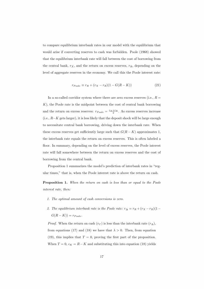
level of aggregate reserves in the economy. We call this the Poole interest rate:
rPoole ≡ rR + (rX − rR)(1−G(R−K)) (21)
In a so-called corridor system where there are zero excess reserves (i.e., R =
K), the Poole rate is the midpoint between the cost of central bank borrowing
and the return on excess reserves: rPoole = rX+rR2 . As excess reserves increase
(i.e., R−K gets larger), it is less likely that the deposit shock will be large enough
to necessitate central bank borrowing, driving down the interbank rate. When
these excess reserves get sufficiently large such that G(R−K) approximates 1,
the interbank rate equals the return on excess reserves. This is often labeled a
floor. In summary, depending on the level of excess reserves, the Poole interest
rate will fall somewhere between the return on excess reserves and the cost of
borrowing from the central bank.
Proposition 1 summarizes the model’s prediction of interbank rates in “reg-
ular times,” that is, when the Poole interest rate is above the return on cash.
Proposition 1. When the return on cash is less than or equal to the Poole
interest rate, then:
1. The optimal amount of cash conversions is zero.
2. The equilibrium interbank rate is the Poole rate: r∆ = rR + (rX − rR)(1−
G(R−K)) = rPoole.
Proof. When the return on cash (rC) is less than the interbank rate (r∆),
from equations (17) and (18) we have that λ > 0. Then, from equation
(19), this implies that T = 0, proving the first part of the proposition.
When T = 0, εK = R−K and substituting this into equation (18) yields
17
r∆ = rPoole. Similarly, according to the first-order conditions, the return
on cash can only equal the Poole rate when λ = 0 and T = 0, in which
case the Poole rate and interbank rate are equal.
We call this the “regular times” scenario because, assuming the return on
cash is nonpositive, this scenario can only arise when the return on excess re-
serves is non-negative, which has been the case for most of history.4 Intuitively,
converting reserves to cash earns commercial banks the return on cash, but
forces them to increase reserves by borrowing on the interbank market at the
Poole rate. If the Poole rate is higher than the return on cash, the profit maxi-
mizing strategy involves zero cash conversions.
Proposition 2. When the return on cash is greater than the Poole interest rate
but less than the cost of central bank borrowing, then:
1. The optimal amount of cash conversions is greater than zero.
2. Cash conversions T adjust until the equilibrium interbank rate is equal to
the return on cash: r∆ = rC .
Proof. Substituting (16) into equation (18), r∆ > rPoole only when T is
greater than zero. When T is greater than zero, it must be the case that
λ = 0, which implies r∆ = rC from equations (17) and (18).
Intuitively, when the return on cash is greater than the Poole interest rate, it
is profitable to convert reserves to cash and make up the shortfall by borrowing
on the interbank market at the Poole rate. But in the presence of cash transfers,
the interbank rate, r∆ = rR+(rX−rR)(1−G(R−K−T )), is similar to the Poole
rate in form but increases in cash transfers T because the likelihood of central
bank borrowing increases. In response, the interbank market rate increases
towards the return on cash. Cash transfers T will increase until the cost of
replacing converted reserves via interbank loans is exactly equal to the return
4We emphasize our use of the Poole rate in proposition 1. It is completely possible forthe Poole rate to be positive and larger than the return on cash even if the return on excessreserves is negative.
18
on cash. Past this point, cash transfers yield a return less than their cost. Thus,
in equilibrium the level of cash transfers T is such that r∆ is equal to rC .
It is important to note that in this framework, when the Poole rate is below
the return on cash, the central bank loses its control of the interbank rate and,
to a certain extent, the level of excess reserves. The interbank rate will be
wholly determined by the return on cash, a rate over which the central bank
generally has no control. Excess reserves are now R − T − K, and although
the central bank can still influence the level of excess reserves by changing the
level of required reserves, K, cash transfers T are wholly determined by the
profit-maximizing commercial banks.
3.3.1 Equilibrium Under Different Monetary Policy Regimes
In the previous section we analyzed equilibrium outcomes when the return on
cash was above or below the Poole rate. In this section we analyze how the
Poole rate changes when the level of aggregate excess reserves, R−K, changes.
We refer to the level of aggregate reserves as the monetary policy regime. A
central bank may explicitly target a specific monetary policy framework, such
as setting R = K = 0 and using a “corridor system.” A central bank may also
prioritize other objectives over strictly controlling the level of excess reserves;
for example, if a central bank operates a Large-Scale Asset Purchase Program
funded by reserves, and does not correspondingly change the level of required
reserves, then the level of excess reserves will be determined by the size of the
asset purchase program.
Figure 2 illustrates how the monetary policy framework interacts with the
Poole rate. The curved line is the Poole rate, which at R = K is exactly the
midpoint between the cost of central bank borrowing and the return on excess
reserves.
The three coloured regions represent the type of equilibrium that occurs for
a given set of interest rates (rX , rR), return on cash (rC), and monetary policy
framework. The region in which the horizontal return on cash line intersects
19
the vertical monetary policy framework line determines the type of equilibrium.
1. Blue region: the return on cash is higher than the cost of borrowing from
the central bank. In this case, the most profitable strategy for a bank
would be to borrow from the central bank and hold that amount as cash.5
2. Green region: the return on cash is higher than the “Poole” rate (but
lower than the cost of borrowing from the central bank), in which case
some cash holdings are optimal.
3. Red region: the return on cash is lower than the overnight rate that would
exist in the absence of cash transfers (the “Poole” rate), which we’ve
already shown will imply zero cash holdings.
The figure’s colours are chosen from the perspective of a commercial bank
making a decision about converting reserves to cash; simply put, the red region
tells the commercial bank not to convert any reserves to cash while the green
region says that some cash holdings are optimal.
Figure 1 shows how the monetary policy framework in place affects which
case arises in equilibrium. Figure 1a is drawn with a hypothetical monetary
policy framework but without the (exogenous) return on cash or equilibrium
interbank rate to clearly illustrate the three distinct cases discussed above. The
horizontal axis represents the monetary policy framework, determined by R−K.
On the far left-hand side, R−K = 0, indicating a corridor system. In this case,
the overnight rate that would exist if cash transfers were not possible, rPoole,
is the midpoint of the central bank borrowing (rX) and deposit (rR) rates. As
R−K increases as one moves towards the right-hand side, we approach a floor
system where rPoole = rR.
If the return on cash is in the red area below rPoole, zero cash conversions
are optimal (case three). In figure 1b, the monetary policy framework, MPF , is
a vertical line and the return on cash, rC , is a horizontal line. The region where
5We do not model this scenario explicitly (instead, central bank borrowing is always theminimum required to meet reserve requirements) since it is highly unlikely to occur and theimplications are obvious.
20
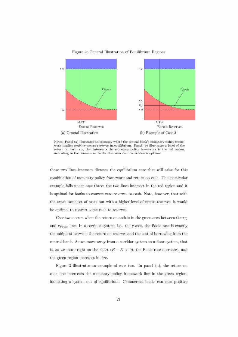
Figure 2: General Illustration of Equilibrium Regions
rX
rR
rPoole
Excess Reserves
MPF
(a) General Illustration
rX
rR
rPoole
Excess Reserves
r∆
rC
MPF
(b) Example of Case 3
Notes: Panel (a) illustrates an economy where the central bank’s monetary policy frame-work implies positive excess reserves in equilibrium. Panel (b) illustrates a level of thereturn on cash, rC , that intersects the monetary policy framework in the red region,indicating to the commercial banks that zero cash conversion is optimal.
these two lines intersect dictates the equilibrium case that will arise for this
combination of monetary policy framework and return on cash. This particular
example falls under case three: the two lines intersect in the red region and it
is optimal for banks to convert zero reserves to cash. Note, however, that with
the exact same set of rates but with a higher level of excess reserves, it would
be optimal to convert some cash to reserves.
Case two occurs when the return on cash is in the green area between the rX
and rPoole line. In a corridor system, i.e., the y-axis, the Poole rate is exactly
the midpoint between the return on reserves and the cost of borrowing from the
central bank. As we move away from a corridor system to a floor system, that
is, as we move right on the chart (R − K > 0), the Poole rate decreases, and
the green region increases in size.
Figure 3 illustrates an example of case two. In panel (a), the return on
cash line intersects the monetary policy framework line in the green region,
indicating a system out of equilibrium. Commercial banks can earn positive
21
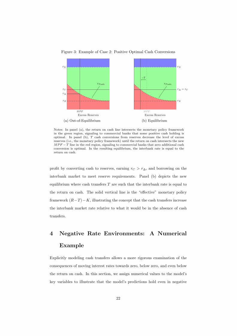
Figure 3: Example of Case 2: Positive Optimal Cash Conversions
rX
rR
rPoole
Excess Reserves
r∆
rC
MPF
(a) Out-of-Equilibrium
rX
rR
rPoole
Excess Reserves
r∆ = rC
MPF
−T
(b) Equilibrium
Notes: In panel (a), the return on cash line intersects the monetary policy frameworkin the green region, signaling to commercial banks that some positive cash holding isoptimal. In panel (b), T cash conversions from reserves decrease the level of excessreserves (i.e., the monetary policy framework) until the return on cash intersects the newMPF −T line in the red region, signaling to commercial banks that zero additional cashconversion is optimal. In the resulting equilibrium, the interbank rate is equal to thereturn on cash.
profit by converting cash to reserves, earning rC > r∆, and borrowing on the
interbank market to meet reserve requirements. Panel (b) depicts the new
equilibrium where cash transfers T are such that the interbank rate is equal to
the return on cash. The solid vertical line is the “effective” monetary policy
framework (R−T )−K, illustrating the concept that the cash transfers increase
the interbank market rate relative to what it would be in the absence of cash
transfers.
4 Negative Rate Environments: A Numerical
Example
Explicitly modeling cash transfers allows a more rigorous examination of the
consequences of moving interest rates towards zero, below zero, and even below
the return on cash. In this section, we assign numerical values to the model’s
key variables to illustrate that the model’s predictions hold even in negative
22
rate environments. We will find that there is nothing intrinsically special about
zero or any other negative number, and, as before, the key rate is the zero-cash-
transfer Poole rate.
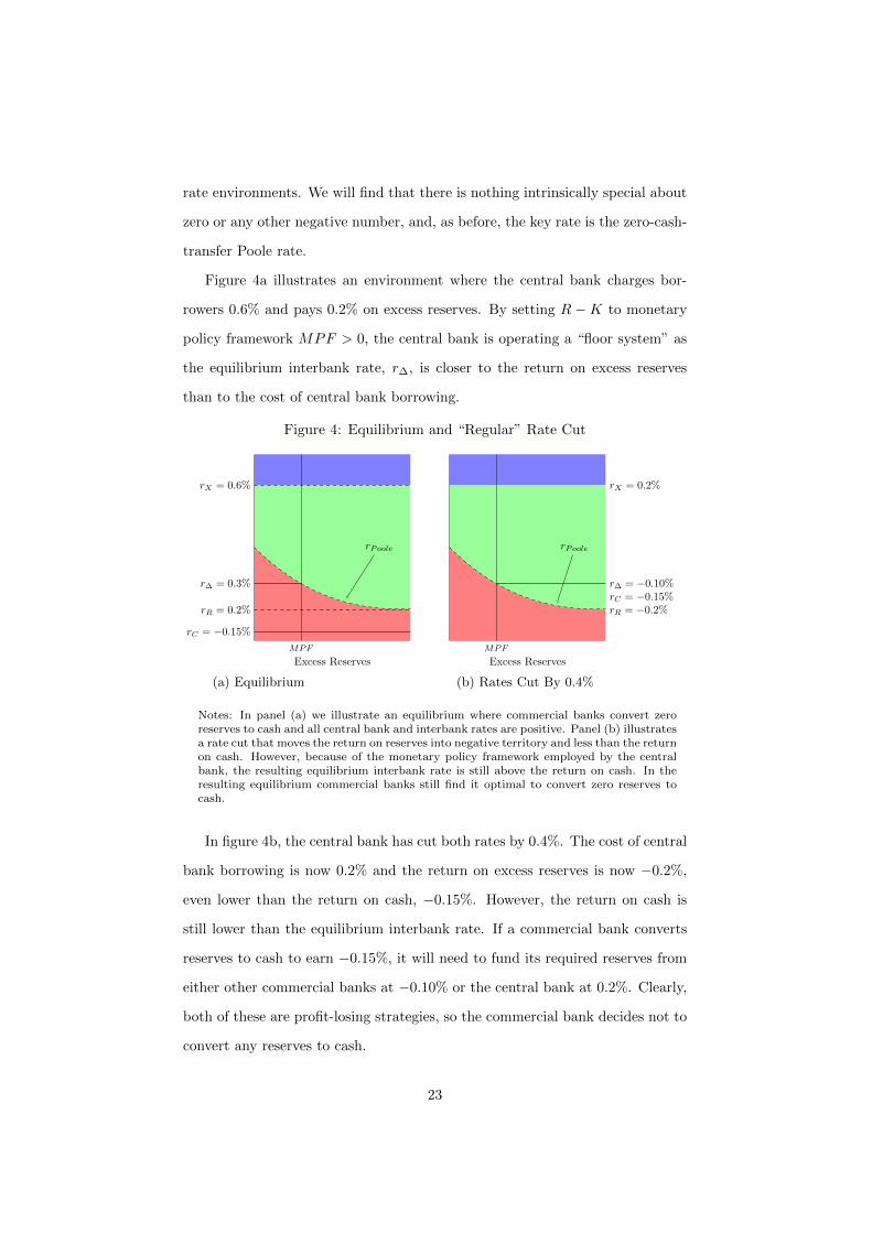
Figure 4a illustrates an environment where the central bank charges bor-
rowers 0.6% and pays 0.2% on excess reserves. By setting R −K to monetary
policy framework MPF > 0, the central bank is operating a “floor system” as
the equilibrium interbank rate, r∆, is closer to the return on excess reserves
than to the cost of central bank borrowing.
Figure 4: Equilibrium and “Regular” Rate Cut
rX = 0.6%
rR = 0.2%
rPoole
Excess Reserves
r∆ = 0.3%
rC = −0.15%
MPF
(a) Equilibrium
rX = 0.2%
rR = −0.2%
rPoole
Excess Reserves
r∆ = −0.10%rC = −0.15%
MPF
(b) Rates Cut By 0.4%
Notes: In panel (a) we illustrate an equilibrium where commercial banks convert zeroreserves to cash and all central bank and interbank rates are positive. Panel (b) illustratesa rate cut that moves the return on reserves into negative territory and less than the returnon cash. However, because of the monetary policy framework employed by the centralbank, the resulting equilibrium interbank rate is still above the return on cash. In theresulting equilibrium commercial banks still find it optimal to convert zero reserves tocash.
In figure 4b, the central bank has cut both rates by 0.4%. The cost of central
bank borrowing is now 0.2% and the return on excess reserves is now −0.2%,
even lower than the return on cash, −0.15%. However, the return on cash is
still lower than the equilibrium interbank rate. If a commercial bank converts
reserves to cash to earn −0.15%, it will need to fund its required reserves from
either other commercial banks at −0.10% or the central bank at 0.2%. Clearly,
both of these are profit-losing strategies, so the commercial bank decides not to
convert any reserves to cash.
23
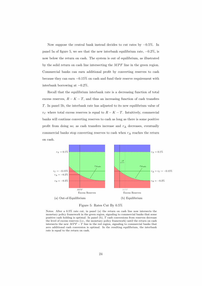
Now suppose the central bank instead decides to cut rates by −0.5%. In
panel 5a of figure 5, we see that the new interbank equilibrium rate, −0.2%, is
now below the return on cash. The system is out of equilibrium, as illustrated
by the solid return on cash line intersecting the MPF line in the green region.
Commercial banks can earn additional profit by converting reserves to cash
because they can earn −0.15% on cash and fund their reserve requirement with
interbank borrowing at −0.2%.
Recall that the equilibrium interbank rate is a decreasing function of total
excess reserves, R − K − T , and thus an increasing function of cash transfers
T . In panel 5b, the interbank rate has adjusted to its new equilibrium value of
rC where total excess reserves is equal to R −K − T . Intuitively, commercial
banks will continue converting reserves to cash as long as there is some positive
profit from doing so; as cash transfers increase and r∆ decreases, eventually
commercial banks stop converting reserves to cash when r∆ reaches the return
on cash.
rX = 0.1%
rR = −0.3%
rPoole
Excess Reserves
r∆ = −0.2%
rC = −0.15%
MPF
(a) Out-of-Equilibrium
rX = 0.1%
rR = −0.3%
rPoole
Excess Reserves
r∆ = rC = −0.15%
MPF
−T
(b) Equilibrium
Figure 5: Rates Cut By 0.5%
Notes: After a 0.5% rate cut, in panel (a) the return on cash line now intersects themonetary policy framework in the green region, signaling to commercial banks that somepositive cash holding is optimal. In panel (b), T cash conversions from reserves decreasethe level of excess reserves (i.e., the monetary policy framework) until the return on cashintersects the new MPF − T line in the red region, signaling to commercial banks thatzero additional cash conversion is optimal. In the resulting equilibrium, the interbankrate is equal to the return on cash.
24
Here we demonstrate the importance of the equilibrium interbank rate, which
is a function not only of the other rates set by the central bank but also of the
monetary policy framework. Under the exact same return on excess reserves
and cost of central bank borrowing, an even higher MPF would have set the
interbank rate even closer to the floor and, in the figure, onto the green area,
which indicates optimal non-zero cash transfers. Thus, a central bank’s op-
erating framework is just as important for the determination of equilibrium
determination as the interest rates it controls.
5 Tiered Remuneration of Central Bank Reserves
In negative rate environments in our model, cash conversions affect the overnight
interbank rate and drive it to equal the return on cash. This may be undesirable
from the central bank’s perspective since the overnight interbank rate is often a
key policy target. In order to maintain control of the interbank rate, the central
bank could disincentivize commercial banks from converting reserves to cash.
We will show that using tiered reserve rates is one way a central bank can use
its existing monetary policy framework to create this disincentive.
In January 2016, the Bank of Japan followed several European central banks
by announcing “a three-tier system in which the outstanding balance of each
financial institution’s current account at the Bank will be divided into three
tiers, to each of which a positive interest rate, a zero interest rate, or a negative
interest rate will be applied, respectively.” In particular, the Bank stated that
“... if a financial institution increases its cash holdings significantly, the bank
will deduct an increase in its cash holdings from the zero interest-rate tiers of
current account balance. Thus, a negative interest rate will be charged on the
increase in its cash holdings.”
Consider a simple numerical example where the return on excess reserves is
−0.40%, the cost of central bank borrowing is 0.10%, and the return on cash is
0%. Suppose there are no aggregate excess reserves while one commercial bank’s
25
required reserves are $0 billion and it currently holds $100 billion in reserves.
The commercial bank will find it profitable to convert the excess $100 billion of
reserves to cash rather than lend to other banks at the midpoint rate of −0.15%.
In doing so, the interbank market is directly affected, and the interbank rate
will simply move to the return on cash. The interbank rate is now determined
completely independently of the monetary policy framework, and the central
bank’s monetary policy is weakened.
The central bank can regain monetary policy efficacy, even with cash trans-
fers, by using the tiered system described above to reduce an amount of re-
serves exempted from being compensated at the lower deposit rate by exactly
the same amount as cash conversions. Recall that the exempted reserves can
be bank-specific, and in reality this is completely plausible since the central
bank maintains an actual account for each commercial bank. By reducing the
exempted reserves amount by the same amount as cash conversions, the excess
reserves remain exactly the same. This is easily seen by combining the following
identities:
reserves = $100 billion− cash conversions
exempted reserves = $50 billion− cash conversions
non-exempted reserves = reserves− exempted reserves
= $50 billion
Note that the amount of reserves above the exemption threshold will always
equal $50 billion, the difference between reserves and exempted reserves, regard-
less of the amount of cash conversions. This is because converting to cash re-
duces reserves, but by reducing the amount of exempted reserves by the amount
of cash converted, such a conversion is essentially neutralized in terms of the
amount of reserves above the threshold requirements. Thus, commercial banks
have a lower incentive to remove reserves from the system.
26
5.1 Modeling Tiered Remuneration of Central Bank Re-
serves
Tiered reserve rates in negative rate environments have two components. The
first is an exemption on paying negative rates on deposits up to a certain thresh-
old, beyond which deposits are compensated at the deposit rate, which would be
negative, so deposits are a cost to banks. The second component is an exemption
threshold that varies depending on the amount of cash withdrawals.
5.1.1 Tiered Remuneration
Modeling this first component requires adapting the framework developed in
section 2. In particular, we do not have a required reserve amount (K = 0)
and the bank is compensated differently on the first M dollars of reserves it
holds at the central bank at the rate rM . Beyond the threshold M, reserves are
compensated at the deposit rate rr.
Assumption 3. The exempted rate is between the central bank lending and
deposit rates: rR < rM ≤ rX .
This means that to be an exemption, the exempted rate, rM , should be
higher than the central bank deposit rate. Above the ceiling on the exempted
rate, banks’ willingness to trade is dependent upon their initial level of reserves
and banks will not necessarily choose their interbank activity depending on the
same critical values. Banks with positive reserves below the threshold and banks
in need of reserves would not have incentive to trade, as they could each receive
a better rate by transacting with the central bank.
In a negative interest rate environment, central banks have typically set
rM = 0, effectively restricting rX ≥ 0. In practice, central banks have not set
their standing facility lending rates below zero in a tiered remuneration system.
Bank profits are still described by equation 6 except that excess reserves up
to M earn rM and all reserves past this threshold earn rR. In expectation, bank
27
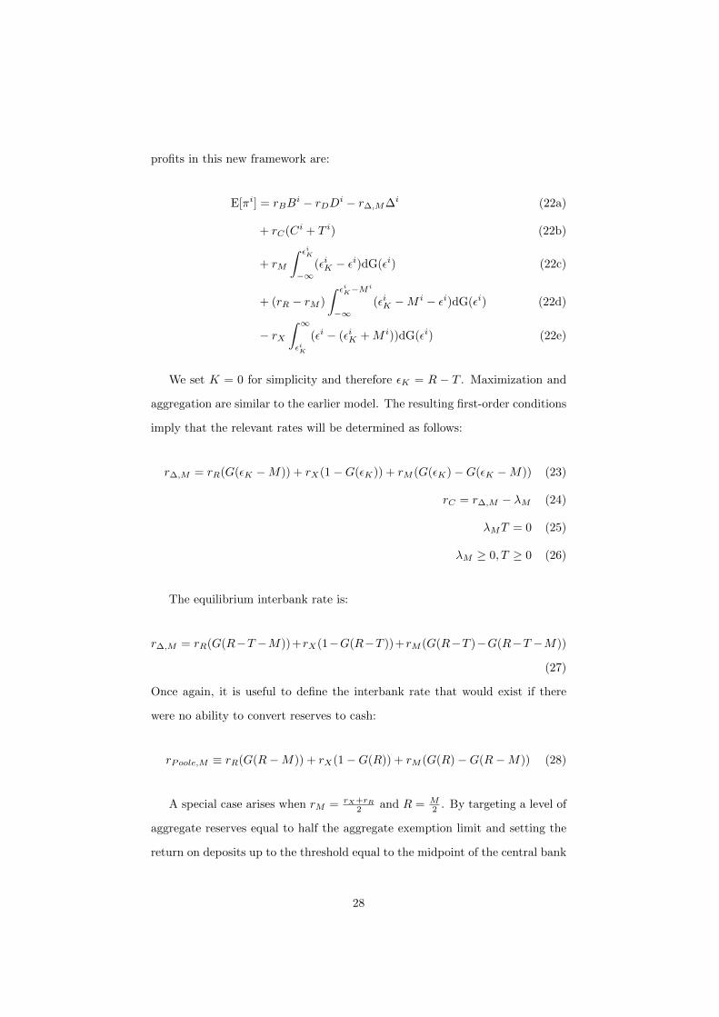
profits in this new framework are:
E[πi] = rBBi − rDDi − r∆,M∆i (22a)
+ rC(Ci + T i) (22b)
+ rM
∫ εiK
−∞(εiK − εi)dG(εi) (22c)
+ (rR − rM )
∫ εiK−Mi
−∞(εiK −M i − εi)dG(εi) (22d)
− rX∫ ∞εiK
(εi − (εiK +M i))dG(εi) (22e)
We set K = 0 for simplicity and therefore εK = R − T . Maximization and
aggregation are similar to the earlier model. The resulting first-order conditions
imply that the relevant rates will be determined as follows:
r∆,M = rR(G(εK −M)) + rX(1−G(εK)) + rM (G(εK)−G(εK −M)) (23)
rC = r∆,M − λM (24)
λMT = 0 (25)
λM ≥ 0, T ≥ 0 (26)
The equilibrium interbank rate is:
r∆,M = rR(G(R−T −M))+rX(1−G(R−T ))+rM (G(R−T )−G(R−T −M))
(27)
Once again, it is useful to define the interbank rate that would exist if there
were no ability to convert reserves to cash:
rPoole,M ≡ rR(G(R−M)) + rX(1−G(R)) + rM (G(R)−G(R−M)) (28)
A special case arises when rM = rX+rR2 and R = M
2 . By targeting a level of
aggregate reserves equal to half the aggregate exemption limit and setting the
return on deposits up to the threshold equal to the midpoint of the central bank
28
lending and borrowing rates, rPoole,M = rPoole. Outside of this example, the
tiered Poole rate will be bounded by the central bank lending and borrowing
rates. However, conversions of reserves to cash could cause the interbank rate
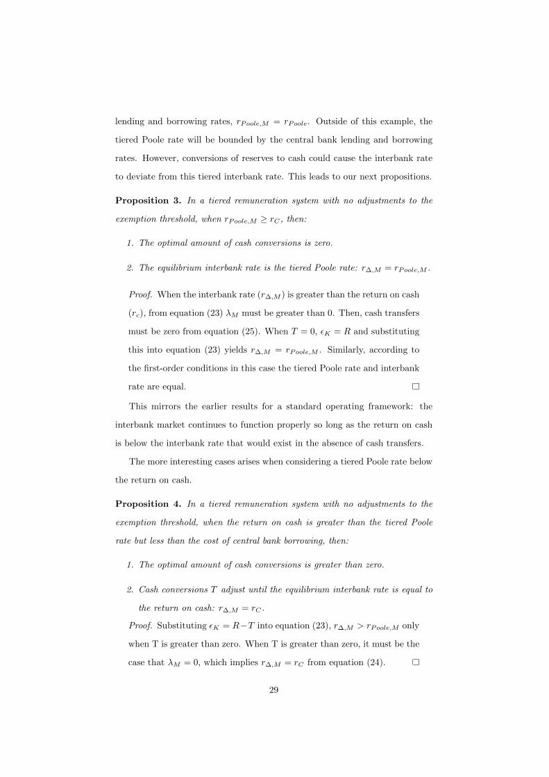
to deviate from this tiered interbank rate. This leads to our next propositions.
Proposition 3. In a tiered remuneration system with no adjustments to the
exemption threshold, when rPoole,M ≥ rC , then:
1. The optimal amount of cash conversions is zero.
2. The equilibrium interbank rate is the tiered Poole rate: r∆,M = rPoole,M .
Proof. When the interbank rate (r∆,M ) is greater than the return on cash
(rc), from equation (23) λM must be greater than 0. Then, cash transfers
must be zero from equation (25). When T = 0, εK = R and substituting
this into equation (23) yields r∆,M = rPoole,M . Similarly, according to
the first-order conditions in this case the tiered Poole rate and interbank
rate are equal.
This mirrors the earlier results for a standard operating framework: the
interbank market continues to function properly so long as the return on cash
is below the interbank rate that would exist in the absence of cash transfers.
The more interesting cases arises when considering a tiered Poole rate below
the return on cash.
Proposition 4. In a tiered remuneration system with no adjustments to the
exemption threshold, when the return on cash is greater than the tiered Poole
rate but less than the cost of central bank borrowing, then:
1. The optimal amount of cash conversions is greater than zero.
2. Cash conversions T adjust until the equilibrium interbank rate is equal to
the return on cash: r∆,M = rC .
Proof. Substituting εK = R−T into equation (23), r∆,M > rPoole,M only
when T is greater than zero. When T is greater than zero, it must be the
case that λM = 0, which implies r∆,M = rC from equation (24).
29
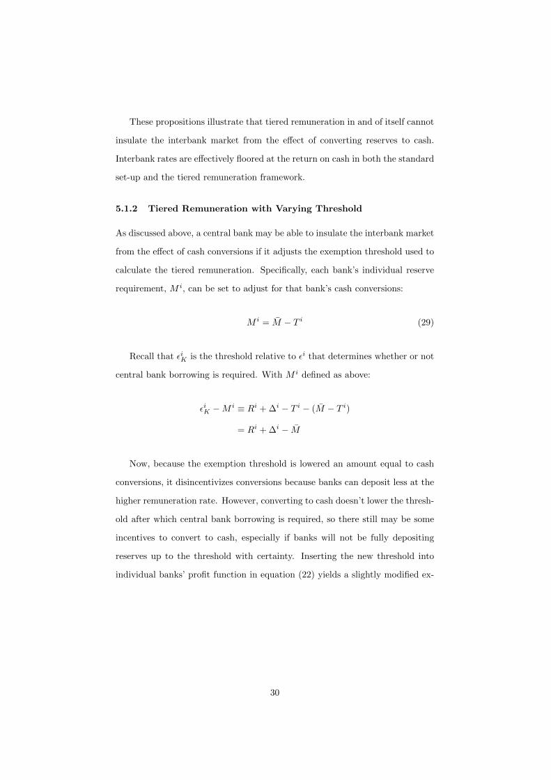
These propositions illustrate that tiered remuneration in and of itself cannot
insulate the interbank market from the effect of converting reserves to cash.
Interbank rates are effectively floored at the return on cash in both the standard
set-up and the tiered remuneration framework.
5.1.2 Tiered Remuneration with Varying Threshold
As discussed above, a central bank may be able to insulate the interbank market
from the effect of cash conversions if it adjusts the exemption threshold used to
calculate the tiered remuneration. Specifically, each bank’s individual reserve
requirement, M i, can be set to adjust for that bank’s cash conversions:
M i = M − T i (29)
Recall that εiK is the threshold relative to εi that determines whether or not
central bank borrowing is required. With M i defined as above:
εiK −M i ≡ Ri + ∆i − T i − (M − T i)
= Ri + ∆i − M
Now, because the exemption threshold is lowered an amount equal to cash
conversions, it disincentivizes conversions because banks can deposit less at the
higher remuneration rate. However, converting to cash doesn’t lower the thresh-
old after which central bank borrowing is required, so there still may be some
incentives to convert to cash, especially if banks will not be fully depositing
reserves up to the threshold with certainty. Inserting the new threshold into
individual banks’ profit function in equation (22) yields a slightly modified ex-
30
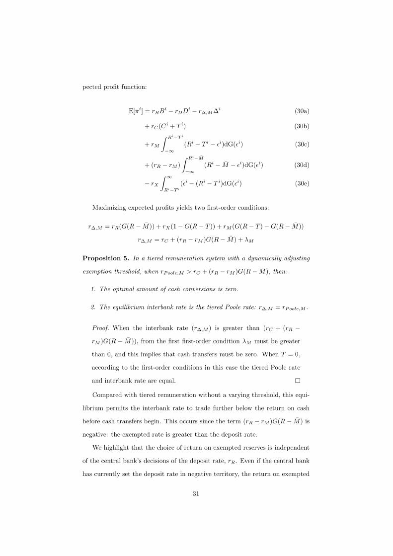
pected profit function:
E[πi] = rBBi − rDDi − r∆,M∆i (30a)
+ rC(Ci + T i) (30b)
+ rM
∫ Ri−T i
−∞(Ri − T i − εi)dG(εi) (30c)
+ (rR − rM )
∫ Ri−M
−∞(Ri − M − εi)dG(εi) (30d)
− rX∫ ∞Ri−T i
(εi − (Ri − T i)dG(εi) (30e)
Maximizing expected profits yields two first-order conditions:
r∆,M = rR(G(R− M)) + rX(1−G(R− T )) + rM (G(R− T )−G(R− M))
r∆,M = rC + (rR − rM )G(R− M) + λM
Proposition 5. In a tiered remuneration system with a dynamically adjusting
exemption threshold, when rPoole,M > rC + (rR − rM )G(R− M), then:
1. The optimal amount of cash conversions is zero.
2. The equilibrium interbank rate is the tiered Poole rate: r∆,M = rPoole,M .
Proof. When the interbank rate (r∆,M ) is greater than (rC + (rR −
rM )G(R − M)), from the first first-order condition λM must be greater
than 0, and this implies that cash transfers must be zero. When T = 0,
according to the first-order conditions in this case the tiered Poole rate
and interbank rate are equal.
Compared with tiered remuneration without a varying threshold, this equi-
librium permits the interbank rate to trade further below the return on cash
before cash transfers begin. This occurs since the term (rR − rM )G(R− M) is
negative: the exempted rate is greater than the deposit rate.
We highlight that the choice of return on exempted reserves is independent
of the central bank’s decisions of the deposit rate, rR. Even if the central bank
has currently set the deposit rate in negative territory, the return on exempted
31
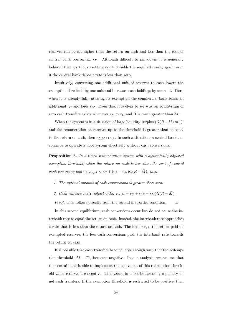
reserves can be set higher than the return on cash and less than the cost of
central bank borrowing, rX . Although difficult to pin down, it is generally
believed that rC ≤ 0, so setting rM ≥ 0 yields the required result, again, even
if the central bank deposit rate is less than zero.
Intuitively, converting one additional unit of reserves to cash lowers the
exemption threshold by one unit and increases cash holdings by one unit. Thus,
when it is already fully utilizing its exemption the commercial bank earns an
additional rC and loses rM . From this, it is clear to see why an equilibrium of
zero cash transfers exists whenever rM > rC and R is much greater than M .
When the system is in a situation of large liquidity surplus (G(R−M) ≈ 1),
and the remuneration on reserves up to the threshold is greater than or equal
to the return on cash, then r∆,M ≈ rR. In such a situation, a central bank can
continue to operate a floor system effectively without cash conversions.
Proposition 6. In a tiered remuneration system with a dynamically adjusted
exemption threshold, when the return on cash is less than the cost of central
bank borrowing and rPoole,M < rC + (rR − rM )G(R− M), then:
1. The optimal amount of cash conversions is greater than zero.
2. Cash conversions T adjust until: r∆,M = rC + (rR − rM )G(R− M).
Proof. This follows directly from the second first-order condition.
In this second equilibrium, cash conversions occur but do not cause the in-
terbank rate to equal the return on cash. Instead, the interbank rate approaches
a rate that is less than the return on cash. The higher rM , the return paid on
exempted reserves, the less cash conversions push the interbank rate towards
the return on cash.
It is possible that cash transfers become large enough such that the redemp-
tion threshold, M − T i, becomes negative. In our analysis, we assume that
the central bank is able to implement the equivalent of this redemption thresh-
old when reserves are negative. This would in effect be assessing a penalty on
net cash transfers. If the exemption threshold is restricted to be positive, then
32
banks would have an incentive to convert reserves to cash if the benefit of doing
so exceeds the lost benefit from utilizing the exemption threshold. This is more
likely to be the case if the exemption threshold is small.
5.1.3 Required Reserves with Varying Threshold
Instead of tiered remuneration of central bank reserves, a central bank could
implement a system of required reserves, where the reserve requirement, Ki,
adjusts depending on the amount of cash withdrawals:
Ki = K − T i (31)
Proposition 7. In a required reserve system with a dynamically adjusting re-
serve requirement, when rK ≥ rC , then:
1. The optimal amount of cash conversions is zero.
2. The equilibrium interbank rate is equal to the target rate: r∆ = rR+(rX−
rR)[1−G(R− K)]
Proof. See Appendix A.
Converting one additional unit of reserves to cash lowers the required reserves
by one unit and increases cash holdings by one unit. Thus, the commercial
bank earns an additional rK and loses rC . From this, it is clear to see why an
equilibrium of zero cash transfers exists whenever rK ≥ rC .
Several central banks have required reserves, so this kind of system should
be relatively straightforward to implement. The advantage of such a system
is that it can produce even tighter control over the overnight rate, given that
the overnight rate is the same as it would be when interest rates are above
the return on cash (i.e., the Poole rate). The choice of return on required
reserves is independent of the central bank’s decisions of the return on (excess)
reserves, rR, and the cost of central bank borrowing, rX . Even if the central
bank has currently set monetary policy in negative territory, the return on
33
required reserves needs only to be higher than the return on cash. Although
difficult to pin down, it is generally believed that rC ≤ 0, so setting rK ≥ 0
yields the required result, again, even if both the return on excess reserves and
the cost of central bank borrowing are both less than zero.
6 Conclusion
Our model illustrates that the lower bound can constrain monetary policy im-
plementation. In particular, the “zero lower bound” on interbank rates isn’t
necessarily at zero, but in fact is determined by the return on cash. Central
bank deposit rates, however, can be below the return on cash.
Tiered remuneration of central bank deposits, in and of itself, does not relax
this constraint much. It is the ability to vary the amount of reserves exempted
from being compensated at the lower deposit rate with the amount of reserves
converted to cash that allows the interbank market to clear at a rate below the
return on cash. The model shows how using a reserve requirement that varies
with conversions of reserves to cash can allow the interbank rate to clear below
the return on cash in a larger number of scenarios.
This model, however, assumes that the central bank is constrained in how it
responds to conversions of reserves to cash. For example, the central bank could
not allow conversions of reserves to cash, which would separate the mechanics
of the overnight market from the return on cash. Nonetheless, it is useful to
examine monetary policy implementation in the absence of such a central bank
response. By adjusting the remuneration of reserves, the model shows that the
central bank can reduce the incentives to convert to cash, lowering the need to
resort to another response.
Finally, our model is focused on the monetary policy implementation aspects
of negative interest rates. The model does not consider the liability side of
bank balance sheets since this is considered beyond scope. For example, retail
depositors could withdraw their deposits if interest rates become too negative.
34

This withdrawal could also influence the banks’ demand for cash from the central
banking sector as well as the compensation banks pay on their deposit liabilities.
This could lower the spread banks earn (Jobst and Lin, 2016). We leave these
questions for future work.
35
References
Gara Afonso and Ricardo Lagos. Trade dynamics in the market for federal
funds. Econometrica, 83(1):263–313, 2015.
Ruchir Agarwal and Miles S Kimball. Breaking through the zero lower bound.
IMF Working Paper, 2015.
Roc Armenter and Benjamin R Lester. Excess reserves and monetary policy
normalization. Federal Reserve Bank of Philadelphia Working Paper No. 16-
33, 2015.
Ryan Banerjee and Hitoshi Mio. The impact of liquidity regulation on banks.
Bank for International Settlements Working Paper No. 470, 2014.
Morten Bech and Todd Keister. Liquidity regulation and the implementation
of monetary policy. Bank for International Settlements Working Paper No.
432, 2013.
Morten Bech and Cyril Monnet. The impact of unconventional monetary policy
on the overnight interbank market.
Morten L Bech and Todd Keister. On the economics of committed liquidity
facilities. Bank for International Settlements Working Paper No. 439, 2014.
Morten L Bech and Elizabeth Klee. The mechanics of a graceful exit: Interest on
reserves and segmentation in the federal funds market. Journal of Monetary
Economics, 58(5):415–431, 2011.
Ulrich Bindseil. Central bank forecasts of liquidity factors: quality, publication
and the control of the overnight rate. European Central Bank Working Paper
No. 70, 2001.
Clemens Bonner and Sylvester CW Eijffinger. The impact of the LCR on the
interbank money market. De Nederlandsche Bank Working Paper No. 364,
2012.
36
Claudio Borio. The implementation of monetary policy in industrial countries:
A survey. Bank for International Settlements Economic Papers No. 47, 1997.
Huberto M Ennis. A simple general equilibrium model of large excess reserves.
Federal Reserve Bank of Richmond Working Paper No. 14-14, 2014.
Benjamin M Friedman and Kenneth N Kuttner. Implementation of monetary
policy: How do central banks set interest rates? Technical report, National
Bureau of Economic Research, 2010.
Marvin Goodfriend. The case for unencumbering interest rate policy at the
zero bound. In Federal Reserve Bank of Kansas City’s 40th Economic Policy
Symposium, Jackson Hole, WY, August, volume 26, 2016.
Cornelia Holthausen, Cyril Monnet, and Flemming Wurtz. Implementing mone-
tary policy without reserve requirements. In Paper for the Financial Seminar
Series, Financial Department, Goethe University, May 27th, 2008.
Jane E Ihrig, Ellen E Meade, and Gretchen C Weinbach. Monetary policy 101:
A primer on the fed’s changing approach to policy implementation. Board of
Governors of the Federal Reserve System Finance and Economics Discussion
Series 2015-047, 2015.
Andreas Jobst and Huidan Lin. Negative Interest Rate Policy (NIRP): Impli-
cations for Monetary Transmission and Bank Profitability in the Euro Area.
International Monetary Fund, 2016.
Anil K Kashyap and Jeremy C Stein. The optimal conduct of monetary policy
with interest on reserves. American Economic Journal: Macroeconomics, 4
(1):266–282, 2012.
Todd Keister and James McAndrews. Why are banks holding so many excess
reserves? Current Issues in Economics and Finance, 15(8), December 2009.
Elizabeth Klee, Zeynep Senyuz, and Emre Yoldas. Effects of changing monetary
and regulatory policy on overnight money markets. Board of Governors of the
37
Federal Reserve System Finance and Economics Discussion Series 2016-084,
2016.
Antoine Martin, James McAndrews, Ali Palida, and David R Skeie. Federal
reserve tools for managing rates and reserves. Federal Reserve Bank of New
York Staff Report No. 642, 2013.
William Poole. Commercial bank reserve management in a stochastic model:
Implications for monetary policy. Journal of Finance, 23(5), 1968.
Marcelo Rezende, Mary-Frances Styczynski, and Cindy Vojtech. The effects
of liquidity regulation on monetary policy implementation. Technical report,
Working paper, Federal Reserve Board, May, 2016.
Gordon H Sellon Jr and Stuart E Weiner. Monetary policy without reserve
requirements: Analytical issues. Economic Review - Federal Reserve Bank of
Kansas City, 81 (4), 1996.
Swiss National Bank. Swiss national bank introduces negative interest rates.
Press Release, December 18, 2014.
Paul Tucker. Managing the central bank’s balance sheet: where monetary policy
meets financial stability. Bank of England Quarterly Bulletin, Autumn, 2004.
Jose Vinals, Simon Gray, and Kelly Eckhold. The broader view: The positive
effects of negative nominal interest rates. iMFdirect blog, April 10, 2016.
William Whitesell. Interest rate corridors and reserves. Journal of Monetary
Economics, 53(6):1177–1195, 2006.
Christopher Whittall and Sam Goldfarb. The black hole of negative rates is
dragging down yields everywhere. Wall Street Journal, July 10, 2016.
Stephen D Williamson. Interest on reserves, interbank lending, and monetary
policy. Federal Reserve Bank of St. Louis Working Paper 2015-024A, 2015.
38

Jonathan Witmer and Jing Yang. Estimating Canada’s effective lower bound.
Bank of Canada Review, 2016(Spring):3–14, 2016.
39
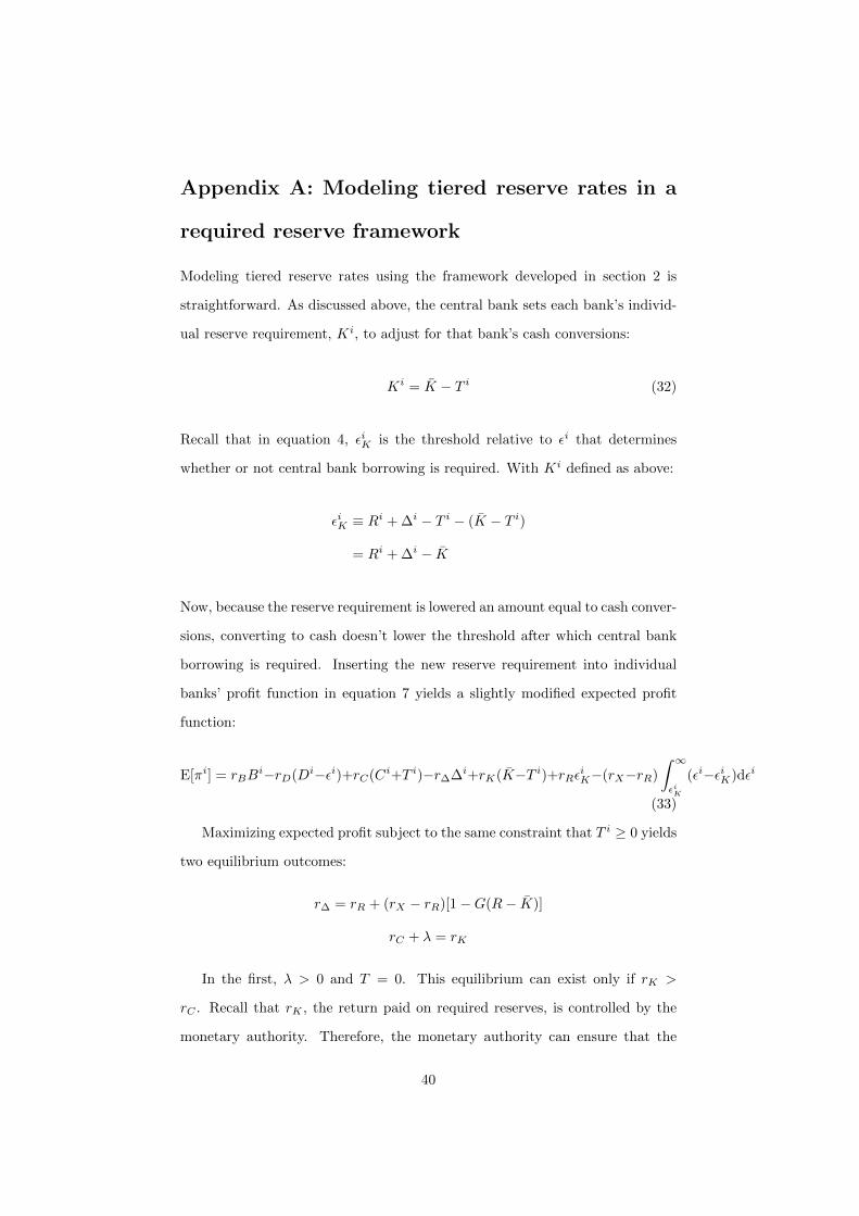
Appendix A: Modeling tiered reserve rates in a
required reserve framework
Modeling tiered reserve rates using the framework developed in section 2 is
straightforward. As discussed above, the central bank sets each bank’s individ-
ual reserve requirement, Ki, to adjust for that bank’s cash conversions:
Ki = K − T i (32)
Recall that in equation 4, εiK is the threshold relative to εi that determines
whether or not central bank borrowing is required. With Ki defined as above:
εiK ≡ Ri + ∆i − T i − (K − T i)
= Ri + ∆i − K
Now, because the reserve requirement is lowered an amount equal to cash conver-
sions, converting to cash doesn’t lower the threshold after which central bank
borrowing is required. Inserting the new reserve requirement into individual
banks’ profit function in equation 7 yields a slightly modified expected profit
function:
E[πi] = rBBi−rD(Di−εi)+rC(Ci+T i)−r∆∆i+rK(K−T i)+rRεiK−(rX−rR)
∫ ∞εiK
(εi−εiK)dεi
(33)
Maximizing expected profit subject to the same constraint that T i ≥ 0 yields
two equilibrium outcomes:
r∆ = rR + (rX − rR)[1−G(R− K)]
rC + λ = rK
In the first, λ > 0 and T = 0. This equilibrium can exist only if rK >
rC . Recall that rK , the return paid on required reserves, is controlled by the
monetary authority. Therefore, the monetary authority can ensure that the
40

bank-specific reserve requirement in equation 32 yields zero cash conversions by
also setting rK > rC . The second equilibrium is when rK = rC and banks are
thus indifferent for any Ti ≥ 0. Clearly, this can easily be avoided by ensuring
that rK > rC .
41