Monetary Policy and Asset PriceVolatility

By Ben Bernanke and Mark Gertler

During the past 20 years, the world’s

major central banks have been largely

successful at bringing inflation under con-

trol. Although it is premature to suggest that infla-

tion is no longer an issue of great concern, it is

quite conceivable that the next battles facing cen-

tral bankers will lie on a different front. One devel-

opment that has already concentrated the minds of

policymakers is an apparent increase in financial

instability, of which one important dimension is

increased volatility of asset prices. Borio, Ken-

nedy, and Prowse (1994), among others, docu-

ment the emergence of major boom-bust cycles

in the prices of equity and real estate in a number

of industrialized countries during the 1980s.

Notable examples include the United States,

Japan, the United Kingdom, the Netherlands,

Sweden, and Finland.

Associated with the “bust” part of the asset

price cycle in many of these cases were signifi-

cant contractions in real economic activity. For

example, many economists attribute at least

some part of the 1990 recession (and the slow

recovery) in the United States to the preced-

ing decline in commercial real estate prices,

which weakened the capital positions of banks

and the balance sheets of corporate borrowers

(Bernanke and Lown). More recently, of

course, we have seen asset price crashes in East

Asia and Latin America, along with continued

stagnation of stock and land prices in Japan, all

of which have been associated with poor eco-

nomic performance. With these experiences in

mind, some observers have viewed the remark-

able rise of the past few years in U.S. stock

prices, and to a lesser extent in real estate

prices, as an ominous development. Of course,

as of this writing, whether the U.S. stock mar-

ket boom will be sustained or will end in tears is

anybody’s guess.

In this paper we address the question of how

central bankers ought to respond to asset price

volatility, in the context of an overall strategy

for monetary policy. To be clear, we agree that

monetary policy is not by itself a sufficient tool

to contain the potentially damaging effects of

booms and busts in asset prices. Well-designed

Ben Bernanke is a professor of economics at Princeton Uni-versity, and Mark Gertler is a professor of economics atNew York University. They presented this paper at the Fed-eral Reserve Bank of Kansas City’s symposium, “NewChallenges for Monetary Policy,”in Jackson Hole, Wyo-ming, August 26-28, 1999. The authors acknowledgeresearch support from the National Science Foundation.Refet Gurkaynak, Matthew Moore, Pau Rabenal, andFederico Ravenna provided excellent research assistance.Rudiger Dornbusch provided useful comments. This articleis on the bank’s web site at www.kc.frb.org.

and transparent legal and accounting systems, a

sound regulatory structure that helps to limit the

risk exposure of banks and corporations, and

prudent fiscal policies that help instill public

confidence in economic fundamentals, are all

vital components of an overall strategy to insu-

late the economy from financial disturbances.

However, our reading of history is that asset

price crashes have done sustained damage to the

economy only in cases when monetary policy

remained unresponsive or actively reinforced

deflationary pressures. This observation is our

justification for focusing on monetary policy here.

The principal argument of the paper is easily

stated. Our view is that, in the context of short-

term monetary policy management, central banks

should view price stability and financial stability

as highly complementary and mutually consis-

tent objectives, to be pursued within a unified

policy framework. In particular, we believe that

the best policy framework for attaining both

objectives is a regime of flexible inflation target-

ing, either of the implicit form now practiced in

the United States or of the more explicit and

transparent type that has been adopted in many

other countries. (We prefer the latter, for reasons

explained briefly at the conclusion of the paper.)

The inflation-targeting approach dictates that cen-

tral banks should adjust monetary policy actively

and pre-emptively to offset incipient inflationary

or deflationary pressures. Importantly, for pres-

ent purposes, it also implies that policy should

not respond to changes in asset prices, except

insofar as they signal changes in expected infla-

tion. Trying to stabilize asset prices per se is prob-

lematic for a variety of reasons, not the least of

which is that it is nearly impossible to know for

sure whether a given change in asset values results

from fundamental factors, nonfundamental fac-

tors, or both. By focusing on the inflationary or

deflationary pressures generated by asset price

movements, a central bank effectively responds

to the toxic side effects of asset booms and busts

without getting into the business of deciding

what is a fundamental and what is not. It also

avoids the historically relevant risk that a bub-

ble, once “pricked,” can easily degenerate into

a panic. Finally, because inflation targeting both

helps to provide stable macroeconomic condi-

tions and also implies that interest rates will

tend to rise during (inflationary) asset price

booms and fall during (deflationary) asset price

busts, this approach may reduce the potential

for financial panics to arise in the first place.

The remainder of the paper is organized as

follows. We begin in Section I with an informal

summary of our views on how asset prices

interact with the real economy and of the associ-

ated implications for monetary policy. To address

these issues more formally, Sections II and III pre-

sent some illustrative policy simulations derived

from a small-scale macroeconomic model that fea-

tures an explicit role for financial conditions in

determining real activity. We move from theory to

practice in Section IV, in which we briefly

examine the recent performance of monetary

policy in the United States and Japan, both of

which have experienced asset price volatility.

Section V concludes with some discussion of

additional issues. The appendix provides more

details of the simulation model employed in

Sections II and III.

I. ASSET PRICES, THE ECONOMY,AND MONETARY POLICY: ANOVERVIEW

Asset prices, including, in particular, the prices

of equities and real estate, are remarkably vari-

able. And although we must not lose sight of

the fact that ultimately asset prices are endoge-

nous variables, there are periods when asset

values seem all but disconnected from the cur-

rent state of the economy. As we noted in the

introduction, during the past two decades econ-

omies across the globe have experienced large

boombust cycles in the prices of various assets,

including equities, commercial real estate, resi-

dential housing, and others.

18 FEDERAL RESERVE BANK OF KANSAS CITY

Should fluctuations in asset prices be of con-

cern to policymakers? In the economist’s usual

benchmark case, a world of efficient capital mar-

kets and without regulatory distortions, move-

ments in asset prices simply reflect changes in

underlying economic fundamentals. Under these

circumstances, central bankers would have no

reason to concern themselves with asset price

volatility per se. Asset prices would be of inter-

est only to the extent that they provide useful

information about the state of the economy.

Matters change, however, if two conditions are

met. The first is that “nonfundamental” factors

sometime underlie asset market volatility. The

second is that changes in asset prices unrelated to

fundamental factors have potentially significant

impacts on the rest of the economy. If these two

conditions are satisfied, then asset price volatil-

ity becomes, to some degree, an independent

source of economic instability, of which policy-

makers should take account.

That both of these conditions hold seems plausi-

ble to us, though there is room for disagreement

on either count. We briefly discuss each in turn.

As potential sources of “nonfundamental” fluc-

tuations in asset prices, at least two possibilities

have been suggested: poor regulatory practice

and imperfect rationality on the part of investors

(“market psychology”). Regarding the former,

Borio and others present evidence for the view that

financial reforms that dramatically increased

access to credit by firms and households contrib-

uted to asset price booms in the 1980s in Scandina-

via, Japan, the Netherlands, the United King-

dom, and elsewhere. Financial liberalizations in

developing countries that have opened the gates

for capital inflows from abroad have also been

associated in some cases with sharply rising asset

values, along with booms in consumption and

lending.

But aren’t liberalizations a good thing? It

depends. As Allen and Gale and others have

emphasized, problems arise when financial lib-

eralizations are not well coordinated with the

regulatory safety net (for example, deposit

insurance and lender-of-last-resort commit-

ments). If liberalization gives additional powers

to private lenders and borrowers while retaining

government guarantees of liabilities, excessive

risk-taking and speculation will follow, leading,

in many cases, to asset price booms. Ultimately,

however, unsound financial conditions are

exposed and lending and asset prices collapse.

This scenario seems to characterize reasonably

well the banking crises recently experienced in a

number of countries, including the United States

and Japan, as well as some of the recent crises in

East Asia and Latin America.

The other possible source of nonfundamental

movements in asset prices that has received

much attention is irrational behavior by inves-

tors, for example, herd behavior, excessive

optimism, or short-termism. There is, of course, a

large amount of literature on bubbles, fads, and

the like. This literature has gained a measure of

credence because of the great difficulty of

explaining the observed level of financial vola-

tility by models based solely on economic fun-

damentals (see, for example, the recent survey by

Campbell). Advocates of bubbles would proba-

bly be forced to admit that it is difficult or impos-

sible to identify any particular episode

conclusively as a bubble, even after the fact.1

Nevertheless, episodes of “irrational exuber-

ance” in financial markets are certainly a logi-

cal possibility, and one about which at least

some central bankers are evidently concerned.

With this concern as motivation, we present

simulations of the economic effects of bubbles

and of alternative policy responses to bubbles

in Section III.

The second necessary condition for asset-

price volatility to be of concern to policymakers

is that booms and busts in asset markets have

important effects on the real economy. Although

the two-way causality between the economy

ECONOMIC REVIEW l FOURTH QUARTER 1999 19

and asset prices makes it difficult to obtain sharp

estimates of the real effects of changes in asset

prices, the historical experience—from the

Great Depression of the 1930s to the most recent

epidemic of crises—is supportive of the view

that large asset price fluctuations can have

important effects on the economy.

What are the mechanisms? One much-cited

possibility is that changes in asset prices affect

consumption spending via their effects on house-

hold wealth. We are not inclined to place a heavy

weight on this channel, however. Empirical stud-

ies (for example, Ludvigson and Steindel;

Parker) have not found a strong or reliable con-

nection between stock market wealth and con-

sumption, for example. This result is, perhaps, not

too surprising, as much of the stock owned by

households is held in pension accounts, implying

that changes in stock values have relatively little

direct impact on spendable cash.

Our own view is that the quantitatively most

important connections between asset prices and

the real economy operate through aspects of

what in earlier work we have called the “balance

sheet channel.”2 The world in which we live, as

opposed to the one envisioned by the benchmark

neoclassical model, is one in which credit mar-

kets are not frictionless; that is, problems of

information, incentives, and enforcement are

pervasive. Because of these problems, credit can

be extended more freely and at lower cost to bor-

rowers who already have strong financial posi-

tions (hence, Ambrose Bierce’s definition of a

banker as someone who lends you an umbrella

when the sun is shining and wants it back when it

starts to rain).

A key implication of the existence of credit-

market frictions is that cash flows and the condi-

tion of balance sheets are important determi-

nants of agents’ ability to borrow and lend.

Research suggests that the effects of asset price

changes on the economy are transmitted to a

very significant extent through their effects on

the balance sheets of households, firms, and

financial intermediaries (see, for example,

Bernanke, Gertler, Gilchrist, forthcoming;

Bernanke and Gertler, 1995). For example,

firms or households may use assets they hold as

collateral when borrowing, in order to amelio-

rate information and incentive problems that

would otherwise interfere with credit extension.

Under such circumstances, a decline in asset

values (for example, a fall in home equity val-

ues) reduces available collateral, leads to an

unplanned increase in leverage on the part of

borrowers, and impedes potential borrowers’

access to credit. Financial intermediaries, which

must maintain an adequate ratio of capital to

assets, can be deterred from lending, or induced

to shift the composition of loans away from

bank-dependent sectors such as small business,

by declines in the values of the assets they hold.

Deteriorating balance sheets and reduced

credit flows operate primarily on spending and

aggregate demand in the short run, although in

the longer run they may also affect aggregate

supply by inhibiting capital formation and

reducing working capital. There also are likely

to be significant feedback and magnification

effects. First, declining sales and employment

imply continuing weakening of cash flows and,

hence, further declines in spending. Bernanke,

Gertler, and Gilchrist (1996) refer to this mag-

nification effect as the “financial accelerator”

(see Bernanke and Gertler, 1989, for an early

formalization). Second, there may also be feed-

back to asset prices, as declining spending and

income, together with forced asset sales, lead to

further decreases in asset values. This “debt-

deflation” mechanism, first described by Irving

Fisher, has been modeled formally by Bernanke

and Gertler (1989), Kiyotaki and Moore, and

Bernanke, Gertler, and Gilchrist (forthcoming).

A large amount of literature has studied the

macroeconomic implications of credit-market

frictions, both theoretically and empirically.3 We

have reviewed that body of research on several

20 FEDERAL RESERVE BANK OF KANSAS CITY

occasions and will not attempt to do so here. We

note, however, that in general this perspective

has proved quite useful for interpreting a number

of historical episodes, including the Great Depres-

sion (Bernanke; Bernanke and James), the deep

Scandinavian recession of the 1980s, the “credit

crunch” episode of 1990-91 in the United States

(Bernanke and Lown), and the protracted weak-

ness of the Japanese economy in the 1990s. A

number of observers (Mishkin; Aghion,

Bacchetta, and Banerjee; Krugman) also have

used this framework to make sense of the fact

that, contrary to conventional wisdom,

exchange-rate devaluations have appeared to be

contractionary in a number of the developing

countries that experienced financial crises in

recent years. The explanation is tied to the fact

that—beguiled by sometimes large interest dif-

ferentials between loans made in foreign and

domestic currencies—banks and corporations in

these countries made liberal use of unhedged,

foreign-currency-denominated debt. The large

devaluations that subsequently occurred raised the

domestic-currency value of these debts, wreak-

ing havoc with bank and corporate balance

sheets and inducing financial distress and major

dislocations in credit, employment, and supplier

relationships.

Beyond providing a mechanism via which

nonfundamental movements in asset prices may

disrupt the economy, a key implication of the

credit-market-frictions perspective is that the

magnitude of the effects of asset-price fluctua-

tions on the economy will depend strongly on

initial financial conditions. By the term, we mean

primarily the initial state of household, firm, and

intermediary balance sheets.4 In particular, the

theory predicts a highly nonlinear effect of asset

prices on spending (Bernanke and Gertler 1989).

Thus, if balance sheets are initially strong, with

low leverage and strong cash flows, then even

rather large declines in asset prices are unlikely

to push households and firms into the region of

financial distress, in which normal access to

credit is jeopardized, or to lead to severe capital

problems for banks. Put another way, the extent

to which an asset-price contraction weakens

private sector balance sheets depends on the

degree and sectoral distribution of initial risk

exposure.

The current (1999) U.S. economy is, we con-

jecture, a case in point. After many years of

expansion, strong profits in both the corporate

and banking sectors, and enormous increases in

the values of equities and other assets, U.S. bal-

ance sheets are in excellent condition. A correc-

tion in the stock market of, say, 25 percent

would, no doubt, slow the economy, but our

guess is that the effects would be relatively tran-

sitory, particularly if monetary policy responds

appropriately. In contrast, a 25 percent decline

in Japanese stock prices, given the parlous con-

dition of its financial system and its seeming

inability to implement a coherent stabilization

policy, would (we expect) create grave and long-

lasting problems for that economy.

If we believe that asset price swings can occur

for nonfundamental reasons, and that these

swings—either through balance-sheet effects

or some other channel—have the potential to

destabilize the real economy, then what are the

implications for monetary policy? As sug-

gested in the introduction, our view is that cen-

tral banks can and should treat price stability

and financial stability as consistent and mutually

reinforcing objectives. In practice, we believe,

this is best accomplished by adopting a strategy

of flexible inflation targeting.5

What is flexible inflation targeting? Although

specific practices differ, broadly speaking, a

regime of inflation targeting has three charac-

teristics. First, as the name suggests, under

inflation targeting, monetary policy is commit-

ted to achieving a specific level of inflation in

the long run, and long-run price stability is des-

ignated the “overriding” or “primary” long-run

goal of policy. Importantly, inflation targeters

are concerned that inflation not be too low as

ECONOMIC REVIEW l FOURTH QUARTER 1999 21

well as that it not be too high; avoidance of defla-

tion is as important (or perhaps even more impor-

tant) as avoidance of high inflation. Second,

within the constraints imposed by the long-run

inflation objective, the central bank has some

flexibility in the short run to pursue other objec-

tives, including output stabilization—hence, the

nomenclature “flexible inflation targeting.”6

Third, inflation targeting is generally character-

ized by substantial openness and transparency

on the part of monetary policymakers, including,

for example, the issuance of regular reports on

the inflation situation and open public discussion

of policy options and plans.

Our characterization of Federal Reserve policy

in recent years is that it meets the first two parts

of the definition of inflation targeting (see Sec-

tion IV for econometric support of this view) but

not the third; that is, the Fed practices “implicit”

rather than “explicit” inflation targeting. Bernanke

and others (1999) argue that the Fed ought to take

the next step and adopt explicit inflation targeting.

For most of the present paper, however, we make

no distinction between implicit and explicit infla-

tion targeting; we return to the issue briefly in the

conclusion.

For our purposes here, the main advantage of

flexible inflation targeting is that it provides a

unified framework both for making monetary

policy in normal times, and for preventing and

ameliorating the effects of financial crises. In

particular, a key advantage of the inflation-

targeting framework is that it induces policy-

makers to automatically adjust interest rates in a

stabilizing direction in the face of asset price

instability or other financial disturbances. The

logic is straightforward; since asset price

increases stimulate aggregate demand and asset

price declines reduce it, the strong focus of infla-

tion targeters on stabilizing aggregate demand

will result in “leaning against the wind”—rais-

ing interest rates as asset prices rise and reducing

them when they fall. This automatic response

not only stabilizes the economy but it is likely to

be stabilizing for financial markets themselves

for several reasons. First, macroeconomic stability,

particularly the absence of inflation or defla-

tion, is itself calming to financial markets.7 Sec-

ond, the central bank’s easing in the face of

asset price declines should help to insulate

balance sheets to some degree, reducing the

economy’s vulnerability to further adverse

shocks. And, finally, if financial-market partici-

pants expect the central bank to behave in this

countercyclical manner, raising interest rates

when asset price increases threaten to overheat

the economy and vice versa, it is possible that

overreactions in asset prices arising from market

psychology and other nonfundamental forces

might be moderated.

The logic of inflation targeting also implies

that central banks should ignore movements in

stock prices that do not appear to be generating

inflationary or deflationary pressures. We con-

cede that forecasting the aggregate demand effects

of asset price movements may not always be an

easy task. However, it is certainly easier than,

first, attempting to distinguish between funda-

mental and nonfundamental fluctuations in asset

prices and, second, attempting to surgically “prick”

the bubble without doing collateral damage to

financial markets or the economy. We explore

the implications of alternative policy responses

to asset price fluctuations in greater detail in the

next two sections.

II. MONETARY POLICY IN THEPRESENCE OF ASSET PRICEBUBBLES: A QUANTITATIVEMODEL

To make the discussion of Section I more

concrete, we will present some model-based

simulations of the performance of alternative

monetary rules in the presence of bubbles in

asset prices. To do this, we extend a small-scale

macroeconomic model developed by Bernanke,

Gertler, and Gilchrist (forthcoming), henceforth

BGG. For the most part, the BGG model is a

22 FEDERAL RESERVE BANK OF KANSAS CITY

standard dynamic new Keynesian model, modi-

fied to allow for financial accelerator effects, as

described in the previous section. Our principal

extension of the BGG model here is to allow for

exogenous bubbles in asset prices.

In this section, we first provide an informal

overview of the BGG model and then describe

how we modify the model to allow for bubbles in

asset prices. The equations of the complete

model are given in the Appendix.8 (Readers who

are not interested in any of this background

material may wish to skip directly to the simula-

tion results in Section III.)

The BGG model

As noted, the foundation of the BGG model is

a standard dynamic new Keynesian framework.

The most important sectors are a household sec-

tor and a business sector. Households are infinitely

lived; they work, consume, and save. Business

firms are owned by entrepreneurs who have

finite expected life.9 There is also a government

that manages fiscal and monetary policy.

Firms own the stock of physical capital,

financing the acquisition of capital through

internally generated funds (primarily revenues

from production and capital gains on assets) and

by borrowing from the public. With their accu-

mulated capital plus hired labor, firms produce

output, which may be used for consumption,

investment, or government purchases. There is

no foreign sector.

Following Taylor (1980), Calvo, and others,

BGG assume the existence of staggered nominal

price setting. The resulting “stickiness” in prices

allows monetary policy to have real effects on

the economy. Optimization and forward-looking

behavior are assumed throughout; the single

exception is the Phillips curve relationship, in

which inflation expectations are modeled as

being formed by a combination of forward- and

backward-looking behavior.10 This modification

increases the persistence of the inflation pro-

cess, allowing a closer fit to the data.

The BGG model differs from this standard

dynamic new Keynesian framework primarily

in assuming the existence of credit-market

frictions, that is, problems of information,

incentives, and enforcement in credit relation-

ships. The presence of these frictions gives rise

to a “financial accelerator” that affects output

dynamics. In particular, in the BGG model,

credit-market frictions make uncollateralized

external finance more expensive than internal

finance. This premium for external finance

affects the overall cost of capital and, thus, the

real investment decisions of firms. The external

finance premium depends inversely on the

financial condition of potential borrowers. For

example, a borrowing firm with more internal

equity can offer more collateral to lenders. Thus,

procyclical movements in the financial condi-

tion of potential borrowers translate into

countercyclical movements in the premium for

external finance, which, in turn, magnify invest-

ment and output fluctuations in the BGG model

(the financial accelerator).

Consider, for example, a shock to the econ-

omy that improves fundamentals, such as a

technological breakthrough. This shock will have

direct effects on output, employment, and the

like. In the BGG model, however, there are also

indirect effects of the shock, arising from the

associated increase in asset prices. Higher asset

prices improve balance sheets, reducing the

external finance premium and further stimulating

investment spending. The increase in invest-

ment may also lead to further increases in asset

prices and cash flows, inducing additional feed-

back effects on spending. Thus, the financial

accelerator enhances the effects of primitive

shocks to the economy.

The financial accelerator mechanism also has

potentially important implications for the work-

ings of monetary policy. As in conventional

ECONOMIC REVIEW l FOURTH QUARTER 1999 23

frameworks, the existence of nominal rigidities

gives the central bank in the BGG model some

control over the short-term real interest rate.

However, beyond the usual neoclassical chan-

nels through which the real interest rate affects

spending, in the BGG model there is an addi-

tional effect that arises from the impact of inter-

est rates on borrower balance sheets. For

example, a reduction in the real interest rate (a

policy easing) raises asset prices, improving the

financial condition of borrowers and reducing

the external finance premium. The reduction in

the premium provides additional stimulus for

investment. BGG find the extra “kick” provided

by this mechanism to be important for explain-

ing the quantitative effects of monetary policy.

Note also that, to the extent that financial crises

are associated with deteriorating private-sector

balance sheets, the BGG framework implies that

monetary policy has a direct means of calming

such crises.

The BGG model assumes that only funda-

mentals drive asset prices, so that the financial

accelerator serves to amplify only fundamen-

tal shocks, such as shocks to productivity or

spending. Our extension of the BGG frame-

work in this paper allows for the possibility

that nonfundamental factors affect asset

prices, which, in turn, affect the real economy

via the financial accelerator.

Adding exogenous asset price bubbles

The fundamental value of capital is the present

value of the dividends the capital is expected to

generate. Formally, define the fundamental value

of depreciable capital in period t Qt, as:

where Et indicates the expectation as of period

t,d is the physical depreciation rate of capital,

D it + are dividends, and Rtq+1

is the relevant sto-

chastic gross discount rate at t for dividends

received in period t +1.

As noted, our principal modification of the

BGG model is to allow for the possibility that

observed equity prices differ persistently from

fundamental values, for example, because of

“bubbles” or “fads.”11 We use the term “bub-

ble” here loosely to denote temporary devia-

tions of asset prices from fundamental values,

due, for example, to liquidity trading or to

waves of optimism or pessimism.12

The key new assumption is that the market

price of capital, S t , may differ from capital’s

fundamental value, Qt . A bubble exists when-

ever S Qt t− ≠ 0. We assume that if a bubble

exists at date t, it persists with probability p and

grows as follows:13

with p a< < 1. If the bubble crashes, with proba-

bility1− p, then

Note that, because a p/ >1, the bubble will

grow until such time as it bursts. For simplicity,

we assume that if a bubble crashes it is not

expected to re-emerge. These assumptions

imply that the expected part of the bubble fol-

lows the process

Because the parameter a is restricted to be

less than unity, the discounted value of the bub-

ble converges to zero over time, with the rate

governed by the value of a.14 That is, bubbles

are not expected to last forever.

Using (2.1) and (2.4) we can derive an

24 FEDERAL RESERVE BANK OF KANSAS CITY

},/])1({[

]/)1[(

111

0

11

0

qtttt

i

j

qjtit

i

itt

RQDE

RDEQ

+++

=++++

∞

=

−+=

−= ∏∑δ

δ

(2.1)

,)( 111

qttttt RQS

p

aQS +++ −=− (2.2)

.011 =− ++ tt QS (2.3)

).()(1

11ttq

t

ttt QSa

R

QSE −=

−

+

++ (2.4)

expression for the evolution of the stock price,

inclusive of the bubble:

where the return on stocks, Rts+1 , is related to the

fundamental return on capital, Rtq+1

, by

and b a≡ −( )1 d .

Equation (2.6) shows that, in the presence of

bubbles, the expected return on stocks will differ

from the return implied by fundamentals. If there

is a positive bubble, S t /Qt >1, the expected

return on stocks will be below the fundamental

return, and vice versa if there is a negative bub-

ble, S t /Qt < 1. However, if the bubble persists

(does not “pop”) a series of supranormal returns

will be observed. This process seems to us to

provide a reasonable description of speculative

swings in the stock market.

The bubble affects real activity in the extended

model in two ways. First, there is a wealth effect

on consumption. Following estimates of the

wealth effect presented in Ludvigson and

Steindel, we parameterize the model so that

these effects are relatively modest (about four

cents of consumption spending for each extra

dollar of stock market wealth). Second, because

the quality of firms’ balance sheets depends on

the market values of their assets rather than the

fundamental values, a bubble in asset prices

affects firms’financial positions and, thus, the pre-

mium for external finance.

Although bubbles in the stock market affect

balance sheets and, thus, the cost of capital, we

continue to assume that—conditional on the cost

of capital—firms make investments based on

fundamental considerations, such as net present

value, rather than on valuations of capital includ-

ing the bubble. This assumption rules out the

arbitrage of building new capital and selling it

at the market price cum bubble (or, equiva-

lently, issuing new shares to finance new capi-

tal). This assumption is theoretically justifiable,

for example, by the lemons premium associated

with new equity issues, and also seems empiri-

cally realistic; see, for example, Bond and

Cummins.

In summary, the main change effected by our

extension of the BGG framework is to allow

nonfundamental movements in asset prices to

influence real activity. Although the source of

the shock may differ, however, the main link

between changes in asset prices and the real

economy remains the financial accelerator, as

in the BGG model.

III. THE IMPACT OF ASSET PRICEFLUCTUATIONS UNDERALTERNATIVE MONETARYPOLICY RULES

In this section we use the extended BGG

model to simulate the effects of asset price bub-

bles and related shocks, such as innovations to

the risk spread, on the economy. Our goal is to

explore what types of policy rules are best at

moderating the disruptive effects of asset mar-

ket disturbances. To foreshadow the results, we

find that a policy rule that is actively focused on

stabilizing inflation seems to work well, and

that this result is reasonably robust across dif-

ferent scenarios.

As a baseline, we assume that the central

bank follows a simple forward-looking policy

rule of the form

where rtn is the nominal instrument interest rate

controlled by the central bank, rn

is the

steady-state value of the nominal interest rate,

and Et tp +1 is the rate of inflation expected in

the next model “period.” We will always

ECONOMIC REVIEW l FOURTH QUARTER 1999 25

},/])1({[ 111

sttttt RSDES +++ −+= δ (2.5)

])1([11

t

tqt

st S

QbbRR −+= ++ (2.6)

,1++= ttnn

t Err πβ (3.1)

assume b>1, so that the central bank responds to

a one percentage point increase in expected infla-

tion by raising the nominal interest rate by more

than one percentage point. This ensures that the

real interest rate increases in the face of rising

expected inflation, so that policy is stabilizing.

The policy rule given by equation (3.1) differs

from the conventional Taylor rule in at least two

ways.15 First, policy is assumed to respond to

anticipations of inflation rather than past values

of inflation. Clarida, Gali, and Gertler (1998,

forthcoming) show that forward-looking reac-

tion functions are empirically descriptive of the

behavior of the major central banks since 1979.

See also the estimates presented in the next sec-

tion of this paper. The second difference from

the standard Taylor rule is that equation (3.1)

omits the usual output gap term. We do this pri-

marily for simplicity and to reduce the number

of dimensions along which the simulations must

be varied. There are a number of rationales for

this omission that are worth brief mention, how-

ever. First, for shocks that primarily affect aggre-

gate demand, such as shocks to asset prices,

rules of the form (3.1) and rules that include an

output gap term will be essentially equivalent in

their effects. Second, as we will see in the next

section, empirical estimates of the responsive-

ness of central banks to the output gap condi-

tional on expected inflation are often rather

small. Finally, assuming for simulation purposes

that the central bank can actually observe the

output gap with precision probably overstates

the case in reality. By leaving out this term we

avoid the issue of how accurately the central

bank can estimate the gap.

Although we do not include the output gap in

the policy rule (3.1), because of our focus on

asset price fluctuations, we do consider a variant

of (3.1) that allows the central bank to respond to

changes in stock prices. Specifically, as an alter-

native to (3.1), we assume that the instrument

rate responds to the once-lagged log level of the

stock price, relative to its steady-state value:

Alternative interpretations of policy rules like

(3.2) are discussed in the next section.

We conducted a variety of simulation experi-

ments, of which we here report an illustrative

sampling. We begin with simulations of the

effects of a stock-market bubble that begins

with an exogenous one percentage point

increase in stock prices (above fundamentals).

We parameterize equation (2.4), which governs

the bubble process, so that the nonfundamental

component of the stock price roughly doubles

each period, as long as the bubble persists.16

The bubble is assumed to last for five periods

and then burst.17 Just before the collapse, the

nonfundamental component is worth about 16

percent of the initial steady state fundamental

value.

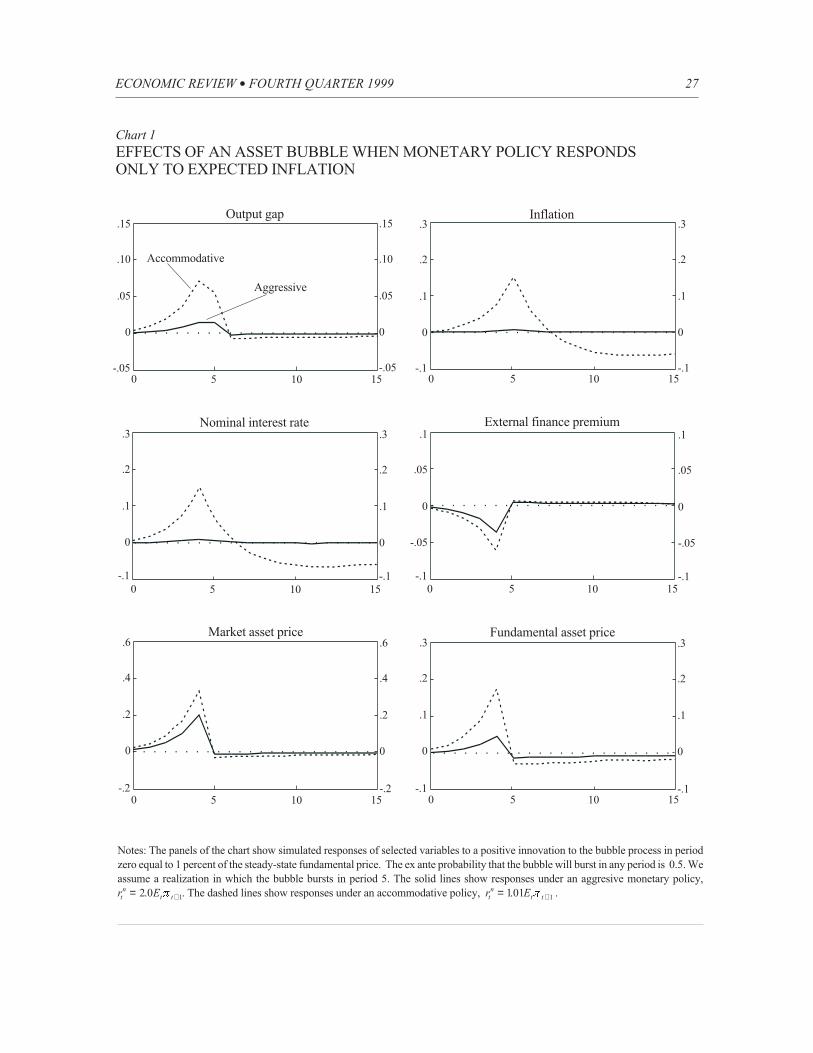
Asset bubbles with policy responding only toinflation. Chart 1 illustrates the simulated

responses of the economy18 to the bubble under

two policy rules of the form (3.1): an “inflation

accommodating” policy for which b +101. and a

more aggressive “inflation targeting” policy for

which b + 20. .19

As Chart 1 shows, under the accommodating

policy, the bubble stimulates aggregate demand,

leading the economy to “overheat.” Inflation and

output rise sharply. The rise in stock prices stimu-

lates spending and output both through the bal-

ance sheet effects described earlier (notice the

decline in the external finance premium in the fig-

ure, which stimulates borrowing) and through

wealth effects on consumption (which are the

relatively less important quantitatively). When

the bubble bursts, there is a corresponding col-

lapse in firms’ net worth. The resulting deterio-

ration in credit markets is reflected in a sharp

increase in the external finance premium (the

spread between firms’ borrowing rates and the

safe rate) and a rapid fall in output. The decline

26 FEDERAL RESERVE BANK OF KANSAS CITY

).log( 11 S

SErr t

ttnn

t−

+ ++= ξπβ (3.2)

ECONOMIC REVIEW l FOURTH QUARTER 1999 27

Chart 1EFFECTS OF AN ASSET BUBBLE WHEN MONETARY POLICY RESPONDSONLY TO EXPECTED INFLATION

Notes: The panels of the chart show simulated responses of selected variables to a positive innovation to the bubble process in period

zero equal to 1 percent of the steady-state fundamental price. The ex ante probability that the bubble will burst in any period is 0.5. We

assume a realization in which the bubble bursts in period 5. The solid lines show responses under an aggresive monetary policy,

r Etn

t t= +2 0 1. p . The dashed lines show responses under an accommodative policy, r Etn

t t= +101 1. p .

.15

.10

-.05

.05

0

.15

.10

-.05

.05

0

Output gap Inflation

External finance premiumNominal interest rate

Fundamental asset priceMarket asset price

Aggressive

Accommodative

.3

.2

-.1

.1

0

.3

.2

-.1

.1

0

.6

.4

-.2

.2

0

.6

.4

-.2

.2

0

.3

.2

-.1

.1

0

.3

.2

-.1

.1

0

.1

.05

-.1

0

-.05

.1

.05

-.1

0

-.05

.3

.2

-.1

.1

0

.3

.2

-.1

.1

0

50 151050 1510

50 151050 1510

50 1510 50 1510

in output after the bursting of the bubble is

greater than the initial expansion, although the

“integral” of output over the episode is positive.

In the absence of further shocks, output does not

continue to spiral downward but stabilizes at a

level just below the initial level of output. Below

we consider scenarios in which the collapse of a

bubble is followed by a financial panic (a nega-

tive bubble), which causes the economy to dete-

riorate further.

In contrast to the accommodative policy, Chart

1 shows that the more aggressive “inflation tar-

geting” policy greatly moderates the effects of

the bubble. Although policy is assumed not to

respond directly to the stock market per se, under

the more aggressive rule, interest rates are

known by the public to be highly responsive to

the incipient inflationary pressures created by

the bubble. The expectation that interest rates

will rise if output and inflation rise is sufficient

both to dampen the response of overall asset

prices to the bubble and to stabilize output and

inflation—even though, ex post, interest rates

are not required to move by as much as in the

accommodative policy.

Asset bubbles with a policy response to stockprices. Chart 2 shows simulation results analo-

gous to those in Chart 1, except that now the cen-

tral bank is allowed to respond directly to stock

prices as well as to expected inflation. We set the

parameter EQUA in equation (3.2) equal to 0.1,

implying that (for constant expected inflation) a

ten-percentage-point rise in the stock market

leads to a one percentage point rise in the instru-

ment rate. Of course, the full response of the

short-term rate to a stock market appreciation is

greater than that, because policy also responds to

the change in expected inflation induced by a

bubble.20

Chart 2 shows that the effect of allowing pol-

icy to respond to stock prices depends greatly on

whether policy is assumed to be accommodating

or aggressive with respect to expected inflation.

Under the accommodating policy b =101. ,

allowing a response to stock prices produces a

perverse outcome. The expectation by the pub-

lic that rates will rise in the wake of the bubble

pushes down the fundamental component of

stock prices, even though overall stock prices

(inclusive of the bubble component) rise.

Somewhat counterintuitively, the rise in rates

and the decline in fundamental values actually

more than offset the stimulative effects of the

bubble, leading output and inflation to

decline—an example of the possible “collat-

eral” damage to the economy that may occur

when the central bank responds to stock prices.

The result that the economy actually contracts,

though a robust one in our simulations, may

rely too heavily on sophisticated forward-look-

ing behavior on the part of private-sector inves-

tors to be entirely plausible as a realistic

description of the actual economy. However,

the general point here is, we think, a valid

one—namely, that a monetary policy regime

that focuses on asset prices rather than on mac-

roeconomic fundamentals may well be actively

destabilizing. The problem is that the central

bank is targeting the wrong indicator.

Under the aggressive policy b = 20. , in con-

trast, allowing policy to respond to the stock

price does little to alter the dynamic responses

of the economy. Evidently, the active compo-

nent of the monetary rule, which strongly

adjusts the real rate to offset movements in

expected inflation, compensates for perverse

effects generated by the response of policy to

stock prices.

To recapitulate, the lesson that we take from

Chart 2 is that it can be quite dangerous for policy

simultaneously to respond to stock prices and to

accommodate inflation. However, when policy

acts aggressively to stabilize expected inflation,

whether policy also responds independently to

stock prices is not of great consequence.

As an alternative metric for evaluating policy

28 FEDERAL RESERVE BANK OF KANSAS CITY

ECONOMIC REVIEW l FOURTH QUARTER 1999 29

Chart 2EFFECTS OF AN ASSET BUBBLE WHEN MONETARY POLICY RESPONDS TOSTOCK PRICES AS WELL AS TO EXPECTED INFLATION

Notes: The panels of the chart show simulated responses of selected variables to a positive innovation to the bubble process, under the

same assumptions as in Chart 1. The solid lines show responses under an aggresive monetary policy, r E stn

t t t= ++ −2 0 011 1. .p . The

dashed lines show responses under an accommodative policy, r E stn

t t t= ++ −101 011 1. .p .

.02

0

-.06

-.02

-.04

.02

0

-.06

-.02

-.04

Output gap Inflation

External finance premiumNominal interest rate

Fundamental asset priceMarket asset price

Aggressive

Accommodative

.5

0

-1.5

-.5

-1

.5

0

-1.5

-.5

-1

.3

.2

-.1

.1

0

.3

.2

-.1

.1

0

.5

0

-1.5

-.5

-1

.5

0

-1.5

-.5

-1

.01

0

-.03

-.01

-.02

.01

0

-.03

-.01

-.02

.1

.05

-.1

0

.05

.1

.05

-.1

0

-.05

50 151050 1510

50 151050 1510

50 1510 50 1510

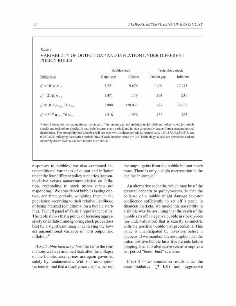
responses to bubbles, we also computed the

unconditional variances of output and inflation

under the four different policy scenarios (accom-

modative versus nonaccommodative on infla-

tion, responding to stock prices versus not

responding). We considered bubbles lasting one,

two, and three periods, weighting them in the

population according to their relative likelihood

of being realized (conditional on a bubble start-

ing). The left panel of Table 1 reports the results.

The table shows that a policy of focusing aggres-

sively on inflation and ignoring stock prices does

best by a significant margin, achieving the low-

est unconditional variance of both output and

inflation.21

Asset bubble then asset bust. So far in the sim-

ulations we have assumed that, after the collapse

of the bubble, asset prices are again governed

solely by fundamentals. With this assumption

we tend to find that a stock-price crash wipes out

the output gains from the bubble but not much

more. There is only a slight overreaction in the

decline in output.22

An alternative scenario, which may be of the

greatest concern to policymakers, is that the

collapse of a bubble might damage investor

confidence sufficiently to set off a panic in

financial markets. We model this possibility in

a simple way by assuming that the crash of the

bubble sets off a negative bubble in stock prices

(an undervaluation) that is exactly symmetric

with the positive bubble that preceded it. This

panic is unanticipated by investors before it

happens. If we maintain the assumption that the

initial positive bubble lasts five periods before

popping, then this alternative scenario implies a

ten-period “boom-bust” scenario.

Chart 3 shows simulation results under the

accommodative ( . )b =101 and aggressive

30 FEDERAL RESERVE BANK OF KANSAS CITY

Table 1

VARIABILITY OF OUTPUT GAP AND INFLATION UNDER DIFFERENTPOLICY RULES

Bubble shock Technology shock

Policy rule: Output gap Inflation Output gap Inflation

r Etn

t t= +101 1. p 2.221 9.676 1.409 17.975

r Etn

t t= +20 1. p 1.471 .119 .103 .231

r E stn

t t t= ++ −101 011 1. .p 5.908 120.032 .987 39.855

r E stn

t t t= ++ −20 011 1. .p 1.518 1.556 .132 .767

Notes: Shown are the unconditional variances of the output gap and inflation under different policy rules, for bubble

shocks and technology shocks. A new bubble starts every period, and its size is randomly drawn from a standard normal

distribution. The probability that a bubble will last one, two, or three periods is, respectively, 0.5/0.875, 0.25/0.875, and

0.25/0.875, reflecting the relative probabilities of each duration when p = 0.5. Technology shocks are permanent and are

randomly drawn from a standard normal distribution.

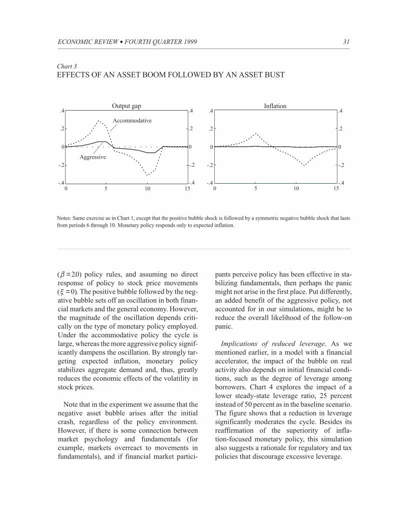
( . )b = 20 policy rules, and assuming no direct

response of policy to stock price movements

( )x = 0 . The positive bubble followed by the neg-

ative bubble sets off an oscillation in both finan-

cial markets and the general economy. However,

the magnitude of the oscillation depends criti-

cally on the type of monetary policy employed.

Under the accommodative policy the cycle is

large, whereas the more aggressive policy signif-

icantly dampens the oscillation. By strongly tar-

geting expected inflation, monetary policy

stabilizes aggregate demand and, thus, greatly

reduces the economic effects of the volatility in

stock prices.

Note that in the experiment we assume that the

negative asset bubble arises after the initial

crash, regardless of the policy environment.

However, if there is some connection between

market psychology and fundamentals (for

example, markets overreact to movements in

fundamentals), and if financial market partici-

pants perceive policy has been effective in sta-

bilizing fundamentals, then perhaps the panic

might not arise in the first place. Put differently,

an added benefit of the aggressive policy, not

accounted for in our simulations, might be to

reduce the overall likelihood of the follow-on

panic.

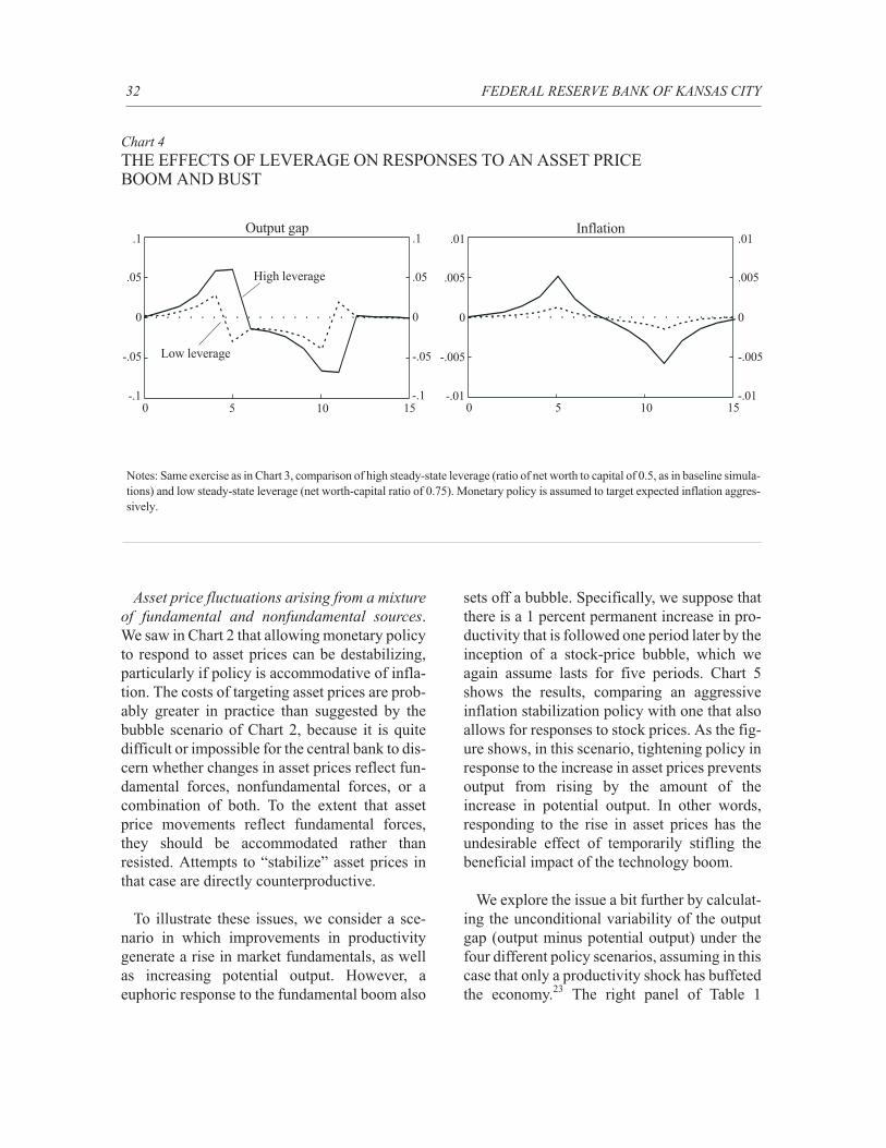
Implications of reduced leverage. As we

mentioned earlier, in a model with a financial

accelerator, the impact of the bubble on real

activity also depends on initial financial condi-

tions, such as the degree of leverage among

borrowers. Chart 4 explores the impact of a

lower steady-state leverage ratio, 25 percent

instead of 50 percent as in the baseline scenario.

The figure shows that a reduction in leverage

significantly moderates the cycle. Besides its

reaffirmation of the superiority of infla-

tion-focused monetary policy, this simulation

also suggests a rationale for regulatory and tax

policies that discourage excessive leverage.

ECONOMIC REVIEW l FOURTH QUARTER 1999 31

.4

.2

-.4

0

-.2

.4

.2

-.4

0

-.2

Output gap Inflation

Aggressive

Accommodative

.4

.2

-.4

0

-.2

.4

.2

-.4

0

-.2

50 151050 1510

Chart 3EFFECTS OF AN ASSET BOOM FOLLOWED BY AN ASSET BUST

Notes: Same exercise as in Chart 1, except that the positive bubble shock is followed by a symmetric negative bubble shock that lasts

from periods 6 through 10. Monetary policy responds only to expected inflation.

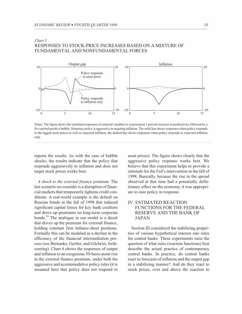
Asset price fluctuations arising from a mixtureof fundamental and nonfundamental sources.

We saw in Chart 2 that allowing monetary policy

to respond to asset prices can be destabilizing,

particularly if policy is accommodative of infla-

tion. The costs of targeting asset prices are prob-

ably greater in practice than suggested by the

bubble scenario of Chart 2, because it is quite

difficult or impossible for the central bank to dis-

cern whether changes in asset prices reflect fun-

damental forces, nonfundamental forces, or a

combination of both. To the extent that asset

price movements reflect fundamental forces,

they should be accommodated rather than

resisted. Attempts to “stabilize” asset prices in

that case are directly counterproductive.

To illustrate these issues, we consider a sce-

nario in which improvements in productivity

generate a rise in market fundamentals, as well

as increasing potential output. However, a

euphoric response to the fundamental boom also

sets off a bubble. Specifically, we suppose that

there is a 1 percent permanent increase in pro-

ductivity that is followed one period later by the

inception of a stock-price bubble, which we

again assume lasts for five periods. Chart 5

shows the results, comparing an aggressive

inflation stabilization policy with one that also

allows for responses to stock prices. As the fig-

ure shows, in this scenario, tightening policy in

response to the increase in asset prices prevents

output from rising by the amount of the

increase in potential output. In other words,

responding to the rise in asset prices has the

undesirable effect of temporarily stifling the

beneficial impact of the technology boom.

We explore the issue a bit further by calculat-

ing the unconditional variability of the output

gap (output minus potential output) under the

four different policy scenarios, assuming in this

case that only a productivity shock has buffeted

the economy.23 The right panel of Table 1

32 FEDERAL RESERVE BANK OF KANSAS CITY

.1

.05

-.1

0

-.05

.1

.05

-.1

0

-.05

Output gap Inflation

Low leverage

High leverage

.01

.005

-.01

0

-.005

.01

.005

-.01

0

-.005

50 151050 1510

Chart 4THE EFFECTS OF LEVERAGE ON RESPONSES TO AN ASSET PRICEBOOM AND BUST

Notes: Same exercise as in Chart 3, comparison of high steady-state leverage (ratio of net worth to capital of 0.5, as in baseline simula-

tions) and low steady-state leverage (net worth-capital ratio of 0.75). Monetary policy is assumed to target expected inflation aggres-

sively.

reports the results. As with the case of bubble

shocks, the results indicate that the policy that

responds aggressively to inflation and does not

target stock prices works best.

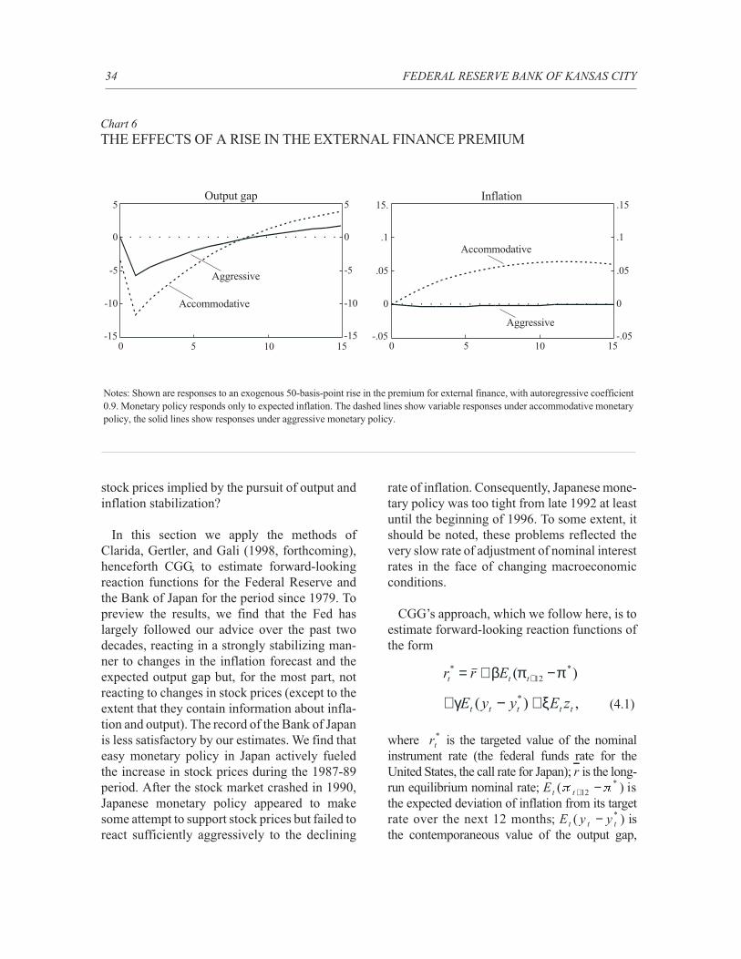
A shock to the external finance premium. The

last scenario we consider is a disruption of finan-

cial markets that temporarily tightens credit con-

ditions. A real-world example is the default on

Russian bonds in the fall of 1998 that induced

significant capital losses for key bank creditors

and drove up premiums on long-term corporate

bonds.24 The analogue in our model is a shock

that drives up the premium for external finance,

holding constant firm balance-sheet positions.

Formally this can be modeled as a decline in the

efficiency of the financial intermediation pro-

cess (see Bernanke, Gertler, and Gilchrist, forth-

coming). Chart 6 shows the responses of output

and inflation to an exogenous 50-basis-point rise

in the external finance premium, under both the

aggressive and accommodative policy rules (it is

assumed here that policy does not respond to

asset prices). The figure shows clearly that the

aggressive policy response works best. We

believe that this experiment helps to provide a

rationale for the Fed’s intervention in the fall of

1998. Basically, because the rise in the spread

observed at that time had a potentially defla-

tionary effect on the economy, it was appropri-

ate to ease policy in response.

IV. ESTIMATED REACTIONFUNCTIONS FOR THE FEDERALRESERVE AND THE BANK OFJAPAN

Section III considered the stabilizing proper-

ties of various hypothetical interest rate rules

for central banks. These experiments raise the

question of what rules (reaction functions) best

describe the actual practice of contemporary

central banks. In practice, do central banks

react to forecasts of inflation and the output gap

in a stabilizing manner? And do they react to

stock prices, over and above the reaction to

ECONOMIC REVIEW l FOURTH QUARTER 1999 33

.01

-.01

0

.01

-.01

0

Output gap Inflation

Policy respondsto inflation only

Policy respondsto asset price

.05

-.05

0

.05

-.05

0

50 151050 1510

Chart 5RESPONSES TO STOCK-PRICE INCREASES BASED ON A MIXTURE OFFUNDAMENTAL AND NONFUNDAMENTAL FORCES

Notes: The figure shows the simulated responses of selected variables to a permanent 1 percent increase in productivity followed by a

five-period positive bubble. Monetary policy is aggressive in targeting inflation. The solid line shows responses when policy responds

to the lagged stock prices as well as expected inflation, the dashed line shows responses when policy responds to expected inflation

only.

stock prices implied by the pursuit of output and

inflation stabilization?

In this section we apply the methods of

Clarida, Gertler, and Gali (1998, forthcoming),

henceforth CGG, to estimate forward-looking

reaction functions for the Federal Reserve and

the Bank of Japan for the period since 1979. To

preview the results, we find that the Fed has

largely followed our advice over the past two

decades, reacting in a strongly stabilizing man-

ner to changes in the inflation forecast and the

expected output gap but, for the most part, not

reacting to changes in stock prices (except to the

extent that they contain information about infla-

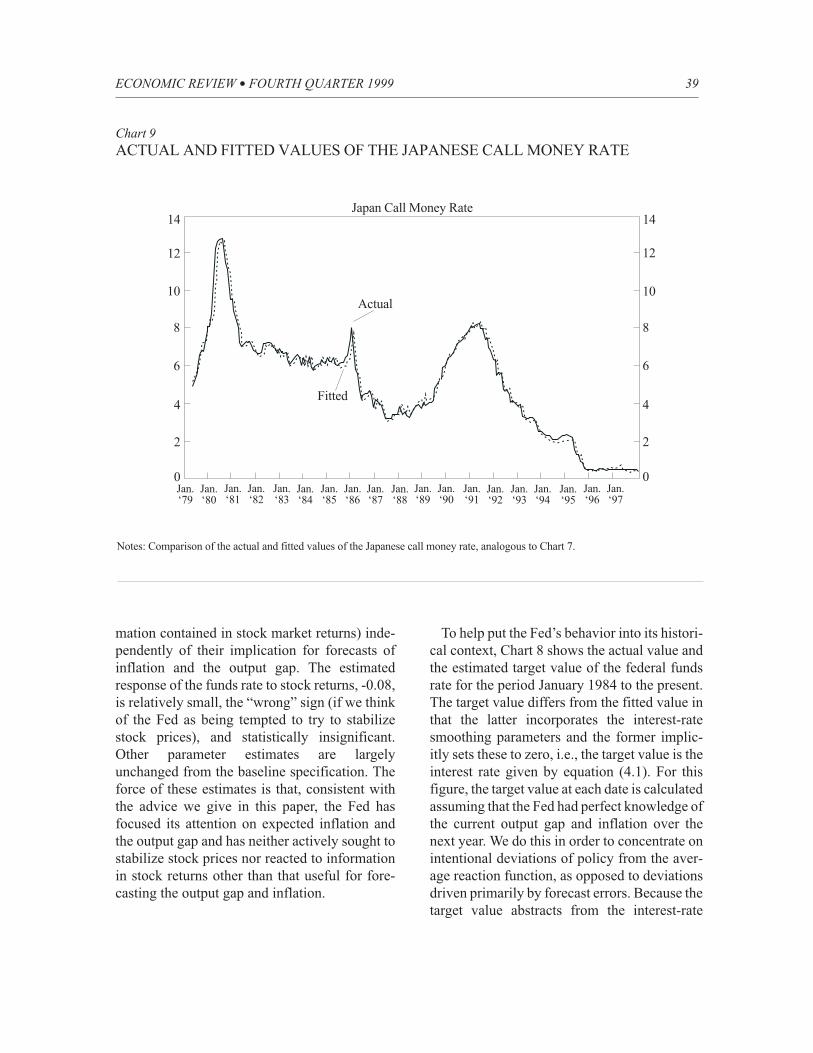
tion and output). The record of the Bank of Japan

is less satisfactory by our estimates. We find that

easy monetary policy in Japan actively fueled

the increase in stock prices during the 1987-89

period. After the stock market crashed in 1990,

Japanese monetary policy appeared to make

some attempt to support stock prices but failed to

react sufficiently aggressively to the declining

rate of inflation. Consequently, Japanese mone-

tary policy was too tight from late 1992 at least

until the beginning of 1996. To some extent, it

should be noted, these problems reflected the

very slow rate of adjustment of nominal interest

rates in the face of changing macroeconomic

conditions.

CGG’s approach, which we follow here, is to

estimate forward-looking reaction functions of

the form

where rt* is the targeted value of the nominal

instrument rate (the federal funds rate for the

United States, the call rate for Japan); r is the long-

run equilibrium nominal rate; Et t( )*p p+ −12 is

the expected deviation of inflation from its target

rate over the next 12 months; E y yt t t( )*− is

the contemporaneous value of the output gap,

34 FEDERAL RESERVE BANK OF KANSAS CITY

5

0

-15

-5

-10

5

0

-15

-5

-10

Output gap Inflation

Accommodative

Aggressive

15.

.1

-.05

.05

0

.15

.1

-.05

.05

0

50 151050 1510

Chart 6THE EFFECTS OF A RISE IN THE EXTERNAL FINANCE PREMIUM

Notes: Shown are responses to an exogenous 50-basis-point rise in the premium for external finance, with autoregressive coefficient

0.9. Monetary policy responds only to expected inflation. The dashed lines show variable responses under accommodative monetary

policy, the solid lines show responses under aggressive monetary policy.

(4.1)

)( *

12

* ππβ −+= +ttt Err

,)( *

ttttt zEyyE ξγ +−+

Aggressive

Accommodative

conditional on information available to the cen-

tral bank at time t; and [equa in text] represents

other variables that may affect the target interest

rate. We expect the parameters b and g to be pos-

itive. CGG point out that stabilization of infla-

tion further requires b>1, i.e., for the real interest

rate to rise when expected inflation rises, the

nominal interest rate must be raised by more than

the increase in expected inflation. In practice, val-

ues of b for central banks with significant

emphasis on inflation stabilization are estimated

to be closer to 2.0. Values less than 1.3 or so indi-

cate a weak commitment to inflation stabiliza-

tion (at these values of b the real interest rate

moves relatively little in response to changes in

expected inflation).

Because of unmodeled motives for interest-

rate smoothing, adjustment of the actual nominal

interest rate toward its target may be gradual.

CGG allow for this by assuming a partial

adjustment mechanism, e.g.,

where rt is the actual nominal interest rate and

p∉ [ , )01 captures the degree of interest-rate

smoothing. Below, we follow CGG in assum-

ing a first-order partial adjustment mechanism,

as in equation (4.2), for Japan and a sec-

ond-order partial adjustment mechanism for the

United States.

To estimate the reaction function implied by

equations (4.1) and (4.2), CGG replace the

expectations of variables in equation (4.1) with

actual realized values of the variables, then

apply an instrumental variables methodology,

ECONOMIC REVIEW l FOURTH QUARTER 1999 35

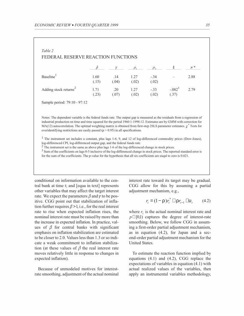
Table 2

FEDERAL RESERVE REACTION FUNCTIONS

b g r1 r2 x p *

Baseline1

1.60

(.15)

.14

(.04)

1.27

(.02)

-.34

(.02)

– 2.88

Adding stock returns2

1.71

(.23)

.20

(.07)

1.27

(.02)

-.33

(.02)

-.0823

(.37)

2.79

Sample period: 79:10 - 97:12

Notes: The dependent variable is the federal funds rate. The output gap is measured as the residuals from a regression of

industrial production on time and time squared for the period 1960:1-1998:12. Estimates are by GMM with correction for

MA(12) autocorrelation. The optimal weighting matrix is obtained from first-step 2SLS parameter estimates. c 2 Tests for

overidentifying restrictions are easily passed (p > 0.95) in all specifications.

1 The instrument set includes a constant, plus lags 1-6, 9, and 12 of log-differenced commodity prices (Dow-Jones),

log-differenced CPI, log-differenced output gap, and the federal funds rate.2 The instrument set is the same as above plus lags 1-6 of the log-differenced change in stock prices.3 Sum of the coefficients on lags 0-5 inclusive of the log-differenced change in stock prices. The reported standard error is

for the sum of the coefficients. The p-value for the hypothesis that all six coefficients are euqal to zero is 0.021.

(4.2)tttt rrr υρρ ++−= −1

*)1(

using as instruments only variables known at

time t-1 or earlier. Under the assumption of ratio-

nal expectations, expectational errors will be

uncorrelated with the instruments, so that the IV

procedure produces consistent estimates of the

reaction function parameters.25

Estimation results are shown in Table 2 for

the Federal Reserve and Table 3 for the Bank of

Japan. Following CGG, we begin the U.S. sam-

ple period in 1979:10, the date of the Volcker

regime shift, and the Japanese sample period in

1979:04, a period CGG refer to as one of “sig-

36 FEDERAL RESERVE BANK OF KANSAS CITY

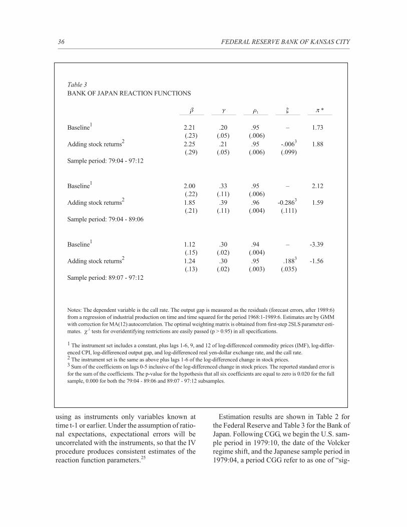
Table 3BANK OF JAPAN REACTION FUNCTIONS

b g r1 x p *

Baseline1

2.21

(.23)

.20

(.05)

.95

(.006)

– 1.73

Adding stock returns2

2.25

(.29)

.21

(.05)

.95

(.006)

-.0063

(.099)

1.88

Sample period: 79:04 - 97:12

Baseline1

2.00

(.22)

.33

(.11)

.95

(.006)

– 2.12

Adding stock returns2

1.85

(.21)

.39

(.11)

.96

(.004)

-0.2863

(.111)

1.59

Sample period: 79:04 - 89:06

Baseline1

1.12

(.15)

.30

(.02)

.94

(.004)

– -3.39

Adding stock returns2

1.24

(.13)

.30

(.02)

.95

(.003)

.1883

(.035)

-1.56

Sample period: 89:07 - 97:12

Notes: The dependent variable is the call rate. The output gap is measured as the residuals (forecast errors, after 1989:6)

from a regression of industrial production on time and time squared for the period 1968:1-1989:6. Estimates are by GMM

with correction for MA(12) autocorrelation. The optimal weighting matrix is obtained from first-step 2SLS parameter esti-

mates. c 2 tests for overidentifying restrictions are easily passed (p > 0.95) in all specifications.

1 The instrument set includes a constant, plus lags 1-6, 9, and 12 of log-differenced commodity prices (IMF), log-differ-

enced CPI, log-differenced output gap, and log-differenced real yen-dollar exchange rate, and the call rate.2 The instrument set is the same as above plus lags 1-6 of the log-differenced change in stock prices.3 Sum of the coefficients on lags 0-5 inclusive of the log-differenced change in stock prices. The reported standard error is

for the sum of the coefficients. The p-value for the hypothesis that all six coefficients are equal to zero is 0.020 for the full

sample, 0.000 for both the 79:04 - 89:06 and 89:07 - 97:12 subsamples.

nificant financial deregulation.” The end date in

each case is 1997:12 (our data end in 1998:12

but we must allow for the fact that one year of

future price change is included on the right-hand

side).26 We also look at two subsamples for

Japan, the periods before and after 1989:6. It was

at the end of 1989 that increases in Bank of Japan

interest rates were followed by the collapse of

stock prices and land values.

For each country and sample period, the tables

report two specifications. As in CGG, the base-

line specification shows the response of the tar-

get for the instrument interest rate to the

expected output gap and expected inflation. The

second, alternative specification adds to the

reaction function the current value and five lags

of the log-difference of an index of the stock

market (the S&P 500 for the United States and

the TOPIX index for Japan). To help control for

simultaneity bias, we instrument for the con-

temporaneous log-difference in the stock mar-

ket index. In particular, we add lags 1 through 6

of the log-difference of the stock market index

to our list of instruments (see endnote 20).

Note, therefore, that in these estimates, the

responses of policy to stock market returns aris-

ing from the predictive power of stock returns

for output and inflation are fully accounted for.

Any estimated response of policy to stock

returns must therefore be over and above the

part due to the predictive power of stock

returns.

ECONOMIC REVIEW l FOURTH QUARTER 1999 37

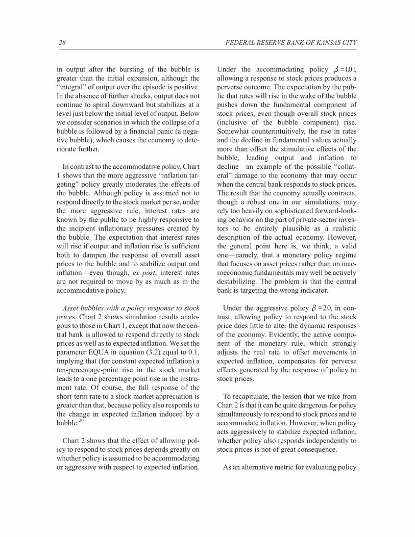
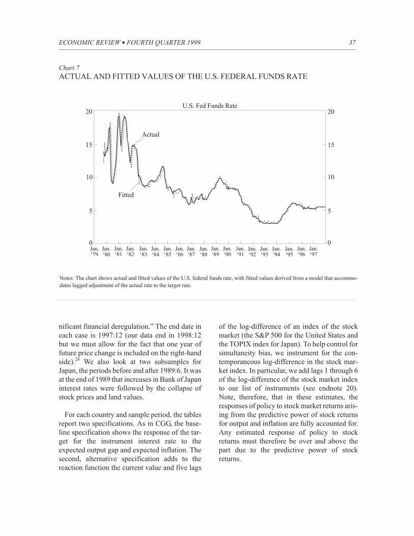
Chart 7ACTUAL AND FITTED VALUES OF THE U.S. FEDERAL FUNDS RATE

Notes: The chart shows actual and fitted values of the U.S. federal funds rate, with fitted values derived from a model that accommo-

dates lagged adjustment of the actual rate to the target rate.

20

0

10

5

15

0

5

10

15

20U.S. Fed Funds Rate

Jan.‘79

Jan.‘81

Jan.‘80

Jan.‘82

Fitted

Jan.‘86

Jan.‘84

Jan.‘85

Jan.‘83

Jan.‘91

Jan.‘93

Jan.‘92

Jan.‘94

Jan.‘90

Jan.‘88

Jan.‘89

Jan.‘87

Jan.‘95

Jan.‘96

Jan.‘97

Actual

There are two ways to think about the addition

of stock market returns to the reaction function.

The first is to interpret it literally as saying that

monetary policy is reacting directly to stock

prices, as well as to the output gap and expected

inflation. The second is to treat the addition of

stock returns as a general specification test that

reveals whether monetary policy is pursuing

other objectives besides stabilization of output

and expected inflation. To the extent that policy

has other objectives, and there is information

about these objectives in the stock market, then

we would expect to see stock returns enter the

central bank’s reaction function with a statisti-

cally significant coefficient.

For the United States, the estimates of the

baseline reaction function (first line of Table 2)

indicate that during the full sample period the

Fed responded reasonably strongly to changes

in forecasted inflation (b =160. ). It also reacted

in a stabilizing manner to forecasts of the out-

put gap ( . )g = 014 . Both parameter estimates are

highly statistically significant. The CGG proce-

dure also permits estimation of the implied tar-

get rate of inflation. For the United States, the

estimated target inflation rate for the full period

is 2.88 percent per year. Chart 7 shows that the

actual and fitted values of the federal funds rate

are very close for the full sample period.27

In the results reported in the second line of

Table 2, we allow for the possibility that the Fed

responded to stock market returns (or to infor-

38 FEDERAL RESERVE BANK OF KANSAS CITY

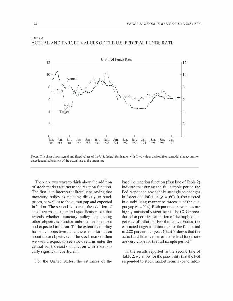
Chart 8ACTUAL AND TARGET VALUES OF THE U.S. FEDERAL FUNDS RATE

Notes: The chart shows actual and fitted values of the U.S. federal funds rate, with fitted values derived from a model that accommo-

dates lagged adjustment of the actual rate to the target rate.

12

0

6

2

10

0

2

6

10

12U.S. Fed Funds Rate

Jan.‘84

Target

Jan.‘86

Jan.‘85

Jan.‘91

Jan.‘93

Jan.‘92

Jan.‘94

Jan.‘90

Jan.‘88

Jan.‘89

Jan.‘87

Jan.‘95

Jan.‘96

Jan.‘97

Actual

88

44

mation contained in stock market returns) inde-

pendently of their implication for forecasts of

inflation and the output gap. The estimated

response of the funds rate to stock returns, -0.08,

is relatively small, the “wrong” sign (if we think

of the Fed as being tempted to try to stabilize

stock prices), and statistically insignificant.

Other parameter estimates are largely

unchanged from the baseline specification. The

force of these estimates is that, consistent with

the advice we give in this paper, the Fed has

focused its attention on expected inflation and

the output gap and has neither actively sought to

stabilize stock prices nor reacted to information

in stock returns other than that useful for fore-

casting the output gap and inflation.

To help put the Fed’s behavior into its histori-

cal context, Chart 8 shows the actual value and

the estimated target value of the federal funds

rate for the period January 1984 to the present.

The target value differs from the fitted value in

that the latter incorporates the interest-rate

smoothing parameters and the former implic-

itly sets these to zero, i.e., the target value is the

interest rate given by equation (4.1). For this

figure, the target value at each date is calculated

assuming that the Fed had perfect knowledge of

the current output gap and inflation over the

next year. We do this in order to concentrate on

intentional deviations of policy from the aver-

age reaction function, as opposed to deviations

driven primarily by forecast errors. Because the

target value abstracts from the interest-rate

ECONOMIC REVIEW l FOURTH QUARTER 1999 39

Chart 9ACTUAL AND FITTED VALUES OF THE JAPANESE CALL MONEY RATE

Notes: Comparison of the actual and fitted values of the Japanese call money rate, analogous to Chart 7.

14

0

6

4

10

0

4

6

10

14Japan Call Money Rate

Jan.‘79

Jan.‘81

Jan.‘80

Jan.‘82

Fitted

Jan.‘86

Jan.‘84

Jan.‘85

Jan.‘83

Jan.‘91

Jan.‘93

Jan.‘92

Jan.‘94

Jan.‘90

Jan.‘88

Jan.‘89

Jan.‘87

Jan.‘95

Jan.‘96

Jan.‘97

Actual

88

1212

2 2

smoothing motive, there is a tendency for the

actual rate to lag somewhat behind the target.

Nevertheless, Chart 8 suggests that the Fed’s

actual choice of short-term rates followed target

rates reasonably closely.

There are, however, three periods of deviation

of the actual fed funds rate from the target rate in

Chart 8 that deserve comment. First, as was

much remarked at the time, the Fed did not ease

policy in 1985-86, even though a sharp decline

in oil prices reduced inflation during those

years.28 The view expressed by some contempo-

rary observers was that the Fed made a con-

scious decision in 1986 to enjoy the beneficial

supply shock in the form of a lower inflation rate

rather than real economic expansion. However,

it is also likely that much of the decline in infla-

tion in 1986 was unanticipated, contrary to the

perfect foresight assumption made in construct-

ing the figure. If true, this would account for

much of the deviation of actual rates from target

in 1985.

Second, the Fed kept rates somewhat below

target in the aftermath of the 1987 stock market

crash. Again, forecasting errors may account

for this deviation. The Fed was concerned at the

time that the depressing effects of the crash

would be larger than, in fact, they turned out

to be.

Finally, and most interesting to us, the Fed

kept the funds rate significantly below target

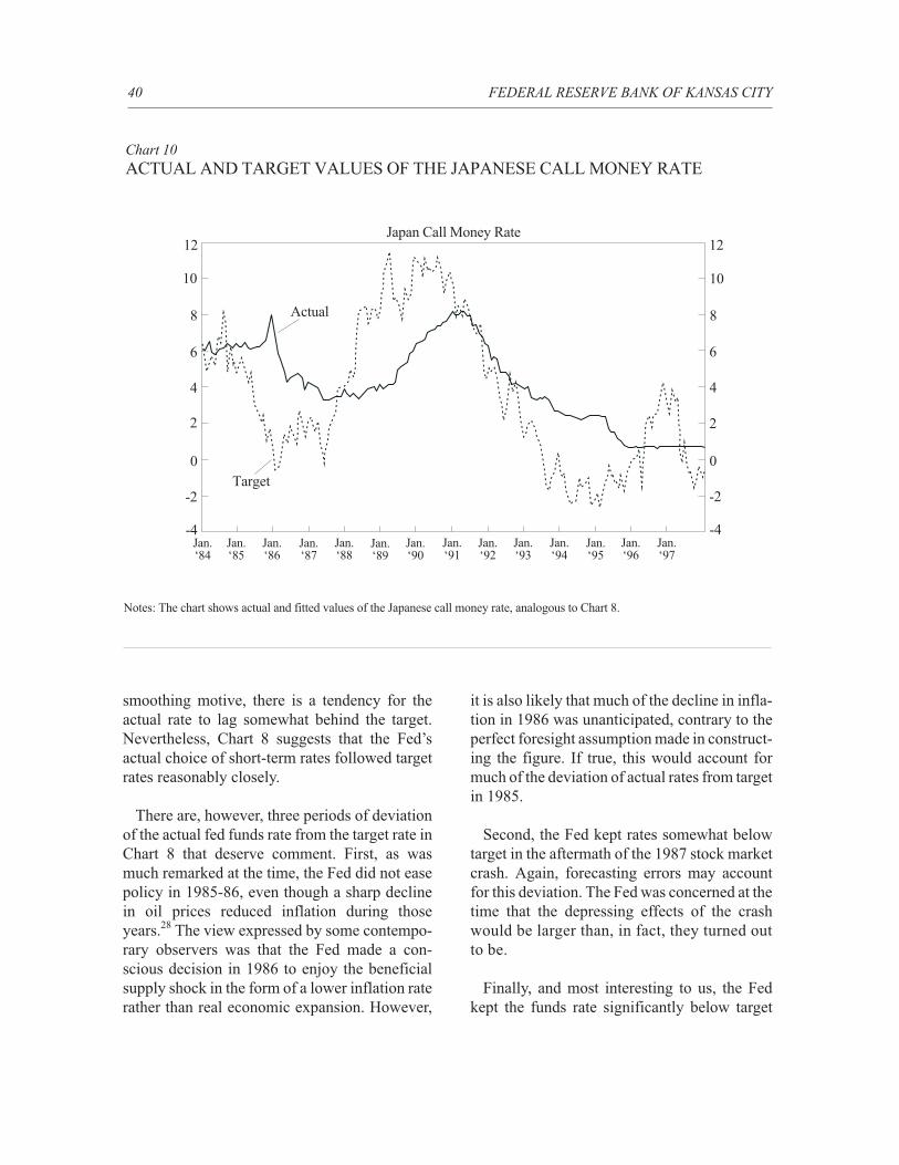
40 FEDERAL RESERVE BANK OF KANSAS CITY

Chart 10ACTUAL AND TARGET VALUES OF THE JAPANESE CALL MONEY RATE

Notes: The chart shows actual and fitted values of the Japanese call money rate, analogous to Chart 8.

12

0

6

2

10

0

2

6

10

12Japan Call Money Rate

Jan.‘84

Target

Jan.‘86

Jan.‘85

Jan.‘91

Jan.‘93

Jan.‘92

Jan.‘94

Jan.‘90

Jan.‘88

Jan.‘89

Jan.‘87

Jan.‘95

Jan.‘96

Jan.‘97

Actual 88

44

-2-2

-4-4

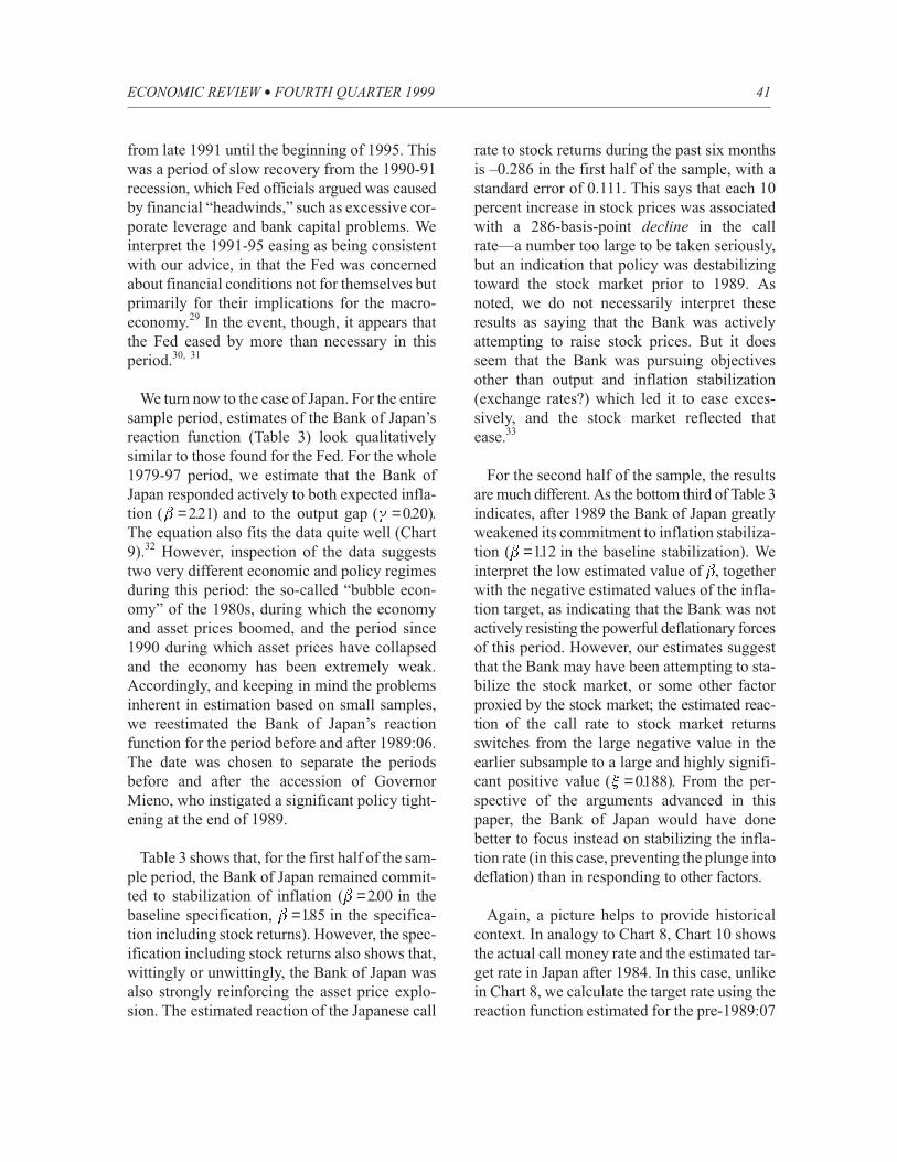
from late 1991 until the beginning of 1995. This

was a period of slow recovery from the 1990-91

recession, which Fed officials argued was caused

by financial “headwinds,” such as excessive cor-

porate leverage and bank capital problems. We

interpret the 1991-95 easing as being consistent

with our advice, in that the Fed was concerned

about financial conditions not for themselves but

primarily for their implications for the macro-

economy.29 In the event, though, it appears that

the Fed eased by more than necessary in this

period.30, 31

We turn now to the case of Japan. For the entire

sample period, estimates of the Bank of Japan’s

reaction function (Table 3) look qualitatively

similar to those found for the Fed. For the whole

1979-97 period, we estimate that the Bank of

Japan responded actively to both expected infla-

tion ( . )b = 221 and to the output gap ( . )g = 020 .

The equation also fits the data quite well (Chart

9).32 However, inspection of the data suggests

two very different economic and policy regimes

during this period: the so-called “bubble econ-

omy” of the 1980s, during which the economy

and asset prices boomed, and the period since

1990 during which asset prices have collapsed

and the economy has been extremely weak.

Accordingly, and keeping in mind the problems

inherent in estimation based on small samples,

we reestimated the Bank of Japan’s reaction

function for the period before and after 1989:06.

The date was chosen to separate the periods

before and after the accession of Governor

Mieno, who instigated a significant policy tight-

ening at the end of 1989.

Table 3 shows that, for the first half of the sam-

ple period, the Bank of Japan remained commit-

ted to stabilization of inflation (b = 200. in the

baseline specification, b =185. in the specifica-

tion including stock returns). However, the spec-

ification including stock returns also shows that,

wittingly or unwittingly, the Bank of Japan was

also strongly reinforcing the asset price explo-

sion. The estimated reaction of the Japanese call

rate to stock returns during the past six months

is –0.286 in the first half of the sample, with a

standard error of 0.111. This says that each 10

percent increase in stock prices was associated

with a 286-basis-point decline in the call

rate—a number too large to be taken seriously,

but an indication that policy was destabilizing

toward the stock market prior to 1989. As

noted, we do not necessarily interpret these

results as saying that the Bank was actively

attempting to raise stock prices. But it does

seem that the Bank was pursuing objectives

other than output and inflation stabilization

(exchange rates?) which led it to ease exces-

sively, and the stock market reflected that

ease.33

For the second half of the sample, the results

are much different. As the bottom third of Table 3

indicates, after 1989 the Bank of Japan greatly

weakened its commitment to inflation stabiliza-

tion (b =112. in the baseline stabilization). We

interpret the low estimated value of b, together

with the negative estimated values of the infla-

tion target, as indicating that the Bank was not

actively resisting the powerful deflationary forces

of this period. However, our estimates suggest

that the Bank may have been attempting to sta-

bilize the stock market, or some other factor

proxied by the stock market; the estimated reac-

tion of the call rate to stock market returns

switches from the large negative value in the

earlier subsample to a large and highly signifi-

cant positive value ( . )x = 0188 . From the per-

spective of the arguments advanced in this

paper, the Bank of Japan would have done

better to focus instead on stabilizing the infla-

tion rate (in this case, preventing the plunge into

deflation) than in responding to other factors.

Again, a picture helps to provide historical

context. In analogy to Chart 8, Chart 10 shows

the actual call money rate and the estimated tar-

get rate in Japan after 1984. In this case, unlike

in Chart 8, we calculate the target rate using the

reaction function estimated for the pre-1989:07

ECONOMIC REVIEW l FOURTH QUARTER 1999 41

sample, without stock returns. This reaction

function seems the right one to use as a bench-

mark because it implies strongly stabilizing

monetary policy, as suggested by the simulations

in the previous section. Thus, the target rate for

the post-1989 period in Chart 10 indicates what

policy would have been if the earlier policies had

been continued, with no attention paid to stock

returns (except as forecasters of the output gap

and inflation).

The results are, again, quite interesting. The

target rate in Japan changed sharply during sev-

eral episodes, and—possibly as a result of an

excessive attachment to interest-rate smooth-

ing—the actual call rate lagged far behind. Chart

10 suggests that policy was, on the whole, rather

tight in Japan during the 1985-87 period, despite

the easing that followed the Plaza Agreement of

September 1985. From 1987 to 1989, however,

Japan faced strong inflationary pressures

(including rocketing asset prices and rapid real

growth), to which the Bank of Japan responded

extremely slowly.34 No doubt, it is this period

that is responsible for our estimated result that

monetary policy actively destabilized the stock

market in the pre-1990 period.

Rates began to rise sharply following the

appointment of Governor Mieno in December

1989, and continued to rise until the spring of

1991. The rate increase was undertaken with the

intention of curbing the stock market and—like

many other attempts to prick market bubbles,

including the U.S. boom in 1929—the attempt

was too successful for the good of the economy.

Asset prices collapsed; and because Japan’s

financial arrangements were particularly sensi-

tive to asset values (we would argue), the real

economy collapsed as well.

Our estimates of the Bank of Japan’s reaction

function for the second half of the sample sug-

gest two countervailing forces. On one hand,

there was now some attempt to stabilize the

stock market, or some factor proxied by the

stock market, by cutting rates as the market fell.

On the other hand, the Bank of Japan’s commit-

ment to stabilizing inflation (here, resisting defla-

tion) seems to have become much weaker. The

net effect was policy that was significantly too

tight, at least until the beginning of 1996.35

We do not want to overstate the conclusions

that can be drawn from this short comparison of

U.S. and Japanese monetary policy since the

mid-1980s. The comparative experience is at

least suggestive, however, that focusing on the

traditional goals of monetary policy—the out-

put gap and expected inflation—is the more

effective means of avoiding extended swings in

asset prices and the resulting damage to the

economy.

V. CONCLUSION

In order to explore the issue of how monetary

policy should respond to variability in asset

prices, we incorporated nonfundamental move-

ments in asset prices into a dynamic macroeco-

nomic framework. To a first approximation at

least, we believe that our framework captures the

main concerns that policymakers have about pos-

sible bubbles in asset prices. In particular, in our

model, a large positive bubble exposes the

economy to the risk of a sharp market correction,

with adverse effects on aggregate demand and

economic activity. In the absence of an appro-

priate policy response, the resulting economic

contraction could be quite large. A severe mar-

ket drop in our model also weakens balance

sheets, induces financial distress, leads to fur-

ther declines in asset prices, and widens spreads

in bond markets. Although our framework omits

some of the microeconomic details of episodes

of stress (for example, nonprice credit rationing,

reduced liquidity of financial markets), and,

hence, is silent about certain types of

lender-of-last- resort interventions that the cen-

tral bank might undertake, we believe that these

omissions are unlikely to affect our central con-

clusions about aggregate stabilization policy.36

42 FEDERAL RESERVE BANK OF KANSAS CITY

The principal conclusion of this paper has

been stated several times. In brief, it is that flexi-

ble inflation-targeting provides an effective, uni-

fied framework for achieving both general

macroeconomic stability and financial stability.

Given a strong commitment to stabilizing

expected inflation, it is neither necessary nor

desirable for monetary policy to respond to

changes in asset prices, except to the extent that

they help to forecast inflationary or deflationary

pressures.

A couple of additional issues deserve very

brief comment. First, our implicit focus in this

paper has been on large industrial economies

such as the United States and Japan. However,

many of the recent financial crises around the

world have occurred in small open economies,

with international capital flows and attacks on

the currency playing major roles. What lessons

does our analysis bear for these countries?

More work would need to be done to extend

our model to the open-economy case, and to

include other sources of financial crisis, such as

speculative attacks on the currency and bank

runs. Such an extension would be worthwhile,

we believe, because it seems to us that bal-

ance-sheet effects of the type captured in the

BGG model have played an important role in

propagating the effects of financial crises

through the real economy. Although we have not

yet done such an extension, one likely conclu-

sion from such an exercise seems obvious

enough and important enough to be worth stating

now; that is: The logic of our approach suggests

strongly that fixed exchange rates, as maintained

by many of the countries recently hit by financial

crises, are highly undesirable in a financially

fragile environment.

The key problem with an exchange-rate peg is

that its defense generally requires movements in

interest rates that are perverse, relative to the

objective of containing a financial crisis. In par-

ticular, the large increases in interest rates neces-

sary to avert devaluation during a currency

crisis exacerbate financial crises both directly,

by depressing asset prices, reducing corporate

profits, and putting pressure on banks, and also

indirectly, by slowing current and expected

rates of economic activity. In addition,

fixed-exchange-rate regimes severely limit the

short-run discretion of the central bank, either

to assist the financial system (for example,

through lender-of-last-resort activities) or to

correct short-term imbalances in the economy.

Indeed, the record of fixed-exchange regimes

in regard to the incidence and severity of finan-

cial crises is notoriously bad.37 During the

Great Depression currency crises (possible, of

course, only if the exchange rate is fixed),

banking panics, and stock market crashes fre-

quently occurred together. Indeed, to the best of

our knowledge, every one of the dozens of

major banking panics of that era occurred in a

country that was attempting to defend a fixed

rate (its gold parity). For the postwar period, in

a study spanning the 1970s through the 1990s,

Kaminsky and Reinhart document that banking

and currency crises frequently occurred

together and appeared to be mutually reinforc-

ing. The strong observed association between

fixed exchange rates and financial crises

appears to be weakened only under two condi-

tions: First, if international capital flows are

highly regulated and restricted, as was the case,

for example, during the Bretton Woods era; or

second, if the international monetary system is

cooperatively managed by the major central

banks, as was arguably the case during the clas-

sical gold standard of the late nineteenth cen-

tury (Eichengreen). Neither of these conditions

prevails today.

So, what should small open economies do?

Our analysis suggests that, if possible, they

adopt flexible inflation targeting as part of a

broad reform package that includes improved

financial regulation and fiscal reform.38 (Brazil

has recently proposed a plan along these lines.)

ECONOMIC REVIEW l FOURTH QUARTER 1999 43

The last part of the recommendation bears

emphasis: Change in the monetary regime alone,

without support from the regulatory and fiscal

arms of government, is not likely to be sufficient.

Moreover, we recognize that successful imple-

mentation of inflation targeting requires both

ample political support from the government and

a certain amount of institutional development,

for example, the existence of adequate price

indexes (see Eichengreen and others). With

these caveats, we recommend that small open

economies head in an inflation-targeting direc-

tion. Note that, along with providing enhanced

macroeconomic and financial stability, a com-

mitment to an inflation-targeting approach by a

small open economy could well deliver greater

long-run stability of the nominal exchange rate

than a regime that attempts to fix the exchange

rate but suffers frequent forced devaluations.

A second broad issue not yet addressed here

concerns the difference between implicit infla-

tion targeting, of the type practiced by the

Greenspan Fed, and explicit inflation targeting,

which involves considerable additional transpar-

ency and communication with the public. It is

evident from recent U.S. experience that implicit

inflation targeting can give good results, and,

indeed, our simulations help to show why a

strong focus on stabilizing expected inflation

promotes overall macroeconomic and financial

stability. We, nevertheless, believe that the United

States would benefit from a move to explicit

inflation targeting, for at least two reasons (see

Bernanke and others 1999, for further discus-

sion). First, making inflation targeting explicit

would serve the important goal of ensuring

continuity in monetary policy, or at least of

increasing the likelihood that future policy

would take the same general approach as recent

policy has taken. In particular, if the infla-

tion-targeting regime were made explicit, the

transition from the current chairman to the next

one would create less anxiety in financial mar-

kets and for the economy than otherwise. Sec-

ond, transparency enhances the stabilizing

properties of forward-looking policies. In par-

ticular, in the simulations reported in this paper

we implicitly assumed transparency of policy,

in that private-sector actors were assumed to

know the policy rule. The results might be very

different if, for example, we assumed that pri-

vate agents thought the central bank was fol-

lowing the accommodative rule when, in fact, it

was following the more aggressive infla-

tion-targeting policy. Likewise, much of the

stabilizing effect of our recommended policy

arises because investors expect the central bank

to raise interest rates when rising asset prices

threaten to overheat the economy, and vice

versa if declining asset prices threaten to induce

an economic contraction. From the standpoint

of maintaining both macroeconomic and finan-

cial stability in the future, the desirability of

increased transparency in U.S. monetary

policymaking is a topic deserving of close

attention in the Fed’s planning.

44 FEDERAL RESERVE BANK OF KANSAS CITY

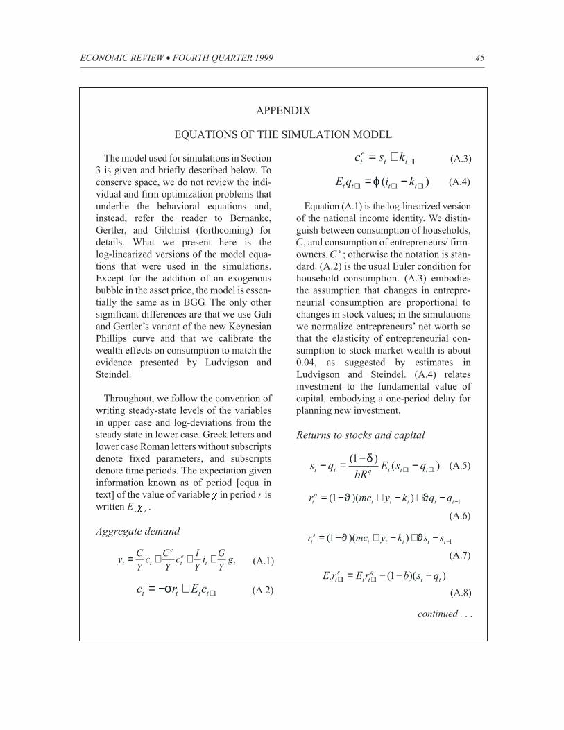
ECONOMIC REVIEW l FOURTH QUARTER 1999 45

APPENDIX

EQUATIONS OF THE SIMULATION MODEL

The model used for simulations in Section

3 is given and briefly described below. To

conserve space, we do not review the indi-

vidual and firm optimization problems that

underlie the behavioral equations and,

instead, refer the reader to Bernanke,

Gertler, and Gilchrist (forthcoming) for

details. What we present here is the

log-linearized versions of the model equa-

tions that were used in the simulations.

Except for the addition of an exogenous

bubble in the asset price, the model is essen-

tially the same as in BGG. The only other

significant differences are that we use Gali

and Gertler’s variant of the new Keynesian

Phillips curve and that we calibrate the

wealth effects on consumption to match the

evidence presented by Ludvigson and

Steindel.

Throughout, we follow the convention of

writing steady-state levels of the variables

in upper case and log-deviations from the

steady state in lower case. Greek letters and

lower case Roman letters without subscripts

denote fixed parameters, and subscripts

denote time periods. The expectation given

information known as of period [equa in

text] of the value of variable c in period r is

written Es rc .

Aggregate demand

Equation (A.1) is the log-linearized version

of the national income identity. We distin-

guish between consumption of households,

C , and consumption of entrepreneurs/ firm-

owners, C e ; otherwise the notation is stan-

dard. (A.2) is the usual Euler condition for

household consumption. (A.3) embodies

the assumption that changes in entrepre-

neurial consumption are proportional to

changes in stock values; in the simulations

we normalize entrepreneurs’ net worth so

that the elasticity of entrepreneurial con-

sumption to stock market wealth is about

0.04, as suggested by estimates in

Ludvigson and Steindel. (A.4) relates

investment to the fundamental value of

capital, embodying a one-period delay for

planning new investment.

Returns to stocks and capital

(A.1)ttet

e

tt gY

Gi

Y

Ic

Y

Cc

Y

Cy +++=

(A.2)1++−= tttt cErc σ

(A.3)1++= ttet ksc

(A.4))( 111 +++ −= tttt kiqE ϕ

)()1(

11 ++ −−=− tttqtt qsEbR

qsδ

(A.5)

1))(1( −−+−+−= tttttq

t qqkymcr ϑϑ

(A.6)

1))(1( −−+−+−= ttttts

t sskymcr ϑϑ

(A.7)

(A.8)

))(1(11 ttq

tts

tt qsbrErE −−−= ++

continued . . .

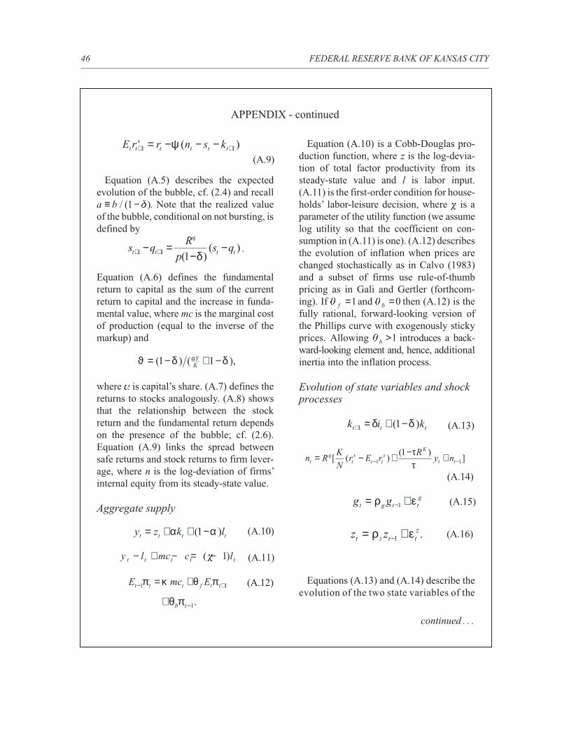
46 FEDERAL RESERVE BANK OF KANSAS CITY

Equation (A.5) describes the expected

evolution of the bubble, cf. (2.4) and recall

a b≡ −/ ( )1 d . Note that the realized value

of the bubble, conditional on not bursting, is

defined by

Equation (A.6) defines the fundamental

return to capital as the sum of the current

return to capital and the increase in funda-

mental value, where mc is the marginal cost

of production (equal to the inverse of the

markup) and

where a is capital’s share. (A.7) defines the

returns to stocks analogously. (A.8) shows

that the relationship between the stock

return and the fundamental return depends

on the presence of the bubble; cf. (2.6).

Equation (A.9) links the spread between

safe returns and stock returns to firm lever-

age, where n is the log-deviation of firms’

internal equity from its steady-state value.

Aggregate supply

Equation (A.10) is a Cobb-Douglas pro-

duction function, where z is the log-devia-

tion of total factor productivity from its

steady-state value and l is labor input.

(A.11) is the first-order condition for house-

holds’ labor-leisure decision, where c is a

parameter of the utility function (we assume

log utility so that the coefficient on con-

sumption in (A.11) is one). (A.12) describes

the evolution of inflation when prices are

changed stochastically as in Calvo (1983)

and a subset of firms use rule-of-thumb

pricing as in Gali and Gertler (forthcom-

ing). If q f =1and q b = 0 then (A.12) is the

fully rational, forward-looking version of

the Phillips curve with exogenously sticky

prices. Allowing q b >1 introduces a back-

ward-looking element and, hence, additional

inertia into the inflation process.

Evolution of state variables and shockprocesses

Equations (A.13) and (A.14) describe the

evolution of the two state variables of the

)()1(

11 tt

q

tt qsp

Rqs −

−=− ++ δ

.

),1()1( δδϑ α −+−= KY

(A.10)tttt lkzy )1( αα −++=

(A.12)11 +− += ttfttt EmcE πθκπ

.1−+ tbπθ

(A.11)y l mc c lt t t t t− + − = −( )c 1

gttgt gg ερ += −1 (A.15)

])1(

)([ 11 −− +−+−= tt

Ks

tts

tq

t nyR

rErN

KRn

ττ

(A.14)

ttt kik )1(1 δδ −+=+ (A.13)

.1

zttzt zz ερ += − (A.16)

continued . . .

APPENDIX - continued

(A.9)

)( 11 ++ −−−= tttts

tt ksnrrE ψ

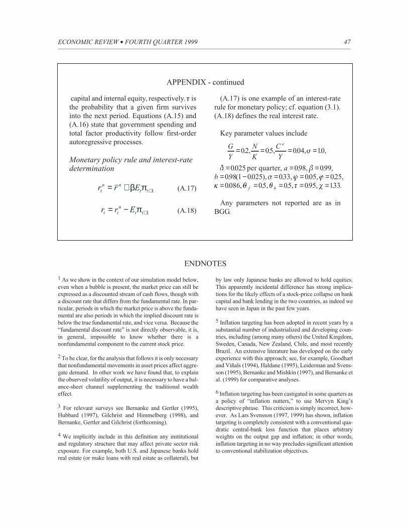
ENDNOTES

1 As we show in the context of our simulation model below,

even when a bubble is present, the market price can still be

expressed as a discounted stream of cash flows, though with

a discount rate that differs from the fundamental rate. In par-

ticular, periods in which the market price is above the funda-

mental are also periods in which the implied discount rate is

below the true fundamental rate, and vice versa. Because the

“fundamental discount rate” is not directly observable, it is,

in general, impossible to know whether there is a

nonfundamental component to the current stock price.

2 To be clear, for the analysis that follows it is only necessary

that nonfundamental movements in asset prices affect aggre-

gate demand. In other work we have found that, to explain

the observed volatility of output, it is necessary to have a bal-

ance-sheet channel supplementing the traditional wealth

effect.

3 For relevant surveys see Bernanke and Gertler (1995),

Hubbard (1997), Gilchrist and Himmelberg (1998), and

Bernanke, Gertler and Gilchrist (forthcoming).

4 We implicitly include in this definition any institutional

and regulatory structure that may affect private sector risk

exposure. For example, both U.S. and Japanese banks hold

real estate (or make loans with real estate as collateral), but

by law only Japanese banks are allowed to hold equities.

This apparently incidental difference has strong implica-

tions for the likely effects of a stock-price collapse on bank

capital and bank lending in the two countries, as indeed we

have seen in Japan in the past few years.

5 Inflation targeting has been adopted in recent years by a

substantial number of industrialized and developing coun-

tries, including (among many others) the United Kingdom,

Sweden, Canada, New Zealand, Chile, and most recently

Brazil. An extensive literature has developed on the early

experience with this approach; see, for example, Goodhart

and Viñals (1994), Haldane (1995), Leiderman and Svens-

son (1995), Bernanke and Mishkin (1997), and Bernanke et

al. (1999) for comparative analyses.

6 Inflation targeting has been castigated in some quarters as

a policy of “inflation nutters,” to use Mervyn King’s

descriptive phrase. This criticism is simply incorrect, how-

ever. As Lars Svensson (1997, 1999) has shown, inflation

targeting is completely consistent with a conventional qua-

dratic central-bank loss function that places arbitrary

weights on the output gap and inflation; in other words,

inflation targeting in no way precludes significant attention

to conventional stabilization objectives.

ECONOMIC REVIEW l FOURTH QUARTER 1999 47

capital and internal equity, respectively. t is

the probability that a given firm survives

into the next period. Equations (A.15) and

(A.16) state that government spending and

total factor productivity follow first-order

autoregressive processes.

Monetary policy rule and interest-ratedetermination

(A.17) is one example of an interest-rate

rule for monetary policy; cf. equation (3.1).

(A.18) defines the real interest rate.

Key parameter values include

G

Y

N

K

C

Y

e

= = = =02 05 004 10. , . , . , . ,s

d = 0025. per quarter, a = =098 099. , . ,bb = − = = =098 1 0025 033 005 025. ( . ), . , . , . ,a y jk q q t c= = = = =0086 05 05 095 133. , . , . , . , . .f b

Any parameters not reported are as in

BGG.

(A.17)1++= ttnn

t Err πβ

(A.18)1+−= ttn

tt Err π

APPENDIX - continued

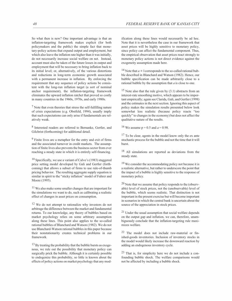
So what then is new? One important advantage is that an

inflation-targeting framework makes explicit (for both

policymakers and the public) the simple fact that mone-

tary-policy actions that expand output and employment, but

which also leave the inflation rate higher than it was initially,

do not necessarily increase social welfare on net. Instead,

account must also be taken of the future losses in output and

employment that will be necessary to bring inflation back to

its initial level; or, alternatively, of the various distortions

and reductions in long-term economic growth associated

with a permanent increase in inflation. By enforcing the

requirement that any sequence of policy actions be consis-

tent with the long-run inflation target (a sort of nominal

anchor requirement), the inflation-targeting framework

eliminates the upward inflation ratchet that proved so costly

in many countries in the 1960s, 1970s, and early 1980s.

7 Note that even theories that stress the self-fulfilling nature

of crisis expectations (e.g. Obstfeld, 1994), usually imply

that such expectations can only arise if fundamentals are rel-

atively weak.

8 Interested readers are referred to Bernanke, Gertler, and

Gilchrist (forthcoming) for additional detail.

9 Finite lives are a metaphor for the entry and exit of firms

and the associated turnover in credit markets. The assump-

tion of finite lives also prevents the business sector from ever

reaching a steady state in which it is entirely self-financing.

10 Specifically, we use a variant of Calvo’s (1983) staggered

price setting model developed by Gali and Gertler (forth-

coming) that allows a subset of firms to use rule-of-thumb

pricing behavior. The resulting aggregate supply equation is

similar in spirit to the “sticky inflation” model of Fuhrer and

Moore (1995).

11 We also make some smaller changes that are important for

the simulations we want to do, such as calibrating a realistic

effect of changes in asset prices on consumption.

12 We do not attempt to rationalize why investors do not

arbitrage the difference between the market and fundamental

returns. To our knowledge, any theory of bubbles based on

market psychology relies on some arbitrary assumption

along these lines. This point also applies to the so-called

rational bubbles of Blanchard and Watson (1982). We do not

use Blanchard-Watson rational bubbles in this paper because

their nonstationarity creates technical problems in our

framework.

13 By treating the probability that the bubble bursts as exoge-

nous, we rule out the possibility that monetary policy can

surgically prick the bubble. Although it is certainly possible

to endogenize this probability, so little is known about the

effects of policy actions on market psychology that any mod-

ification along these lines would necessarily be ad hoc.

Note that it is nevertheless the case in our framework that

asset prices will be highly sensitive to monetary policy,

since policy can affect the fundamental component. Thus,

the empirical observation that asset prices react strongly to

monetary policy actions is not direct evidence against the

exogeneity assumption made here.

14 Note that a = 1corresponds to the so-called rational bub-

ble described in Blanchard and Watson (1982). Hence, our

bubble specification can be made arbitrarily close to a

rational bubble by the assumption that a is close to one.

15 Note also that the rule given by (3.1) abstracts from an

interest-rate smoothing motive, which appears to be impor-

tant empirically; again see Clarida, Gali, and Gertler (1998)

and the estimates in the next section. Ignoring this aspect of

policy makes the simulation results presented below look

somewhat less realistic (because policy reacts “too

quickly” to changes in the economy) but does not affect the

qualitative nature of the results.

16 We assume p = 0.5 and a = 0.98.

17 To be clear, agents in the model know only the ex ante

stochastic process for the bubble and not the time that it will

burst.

18 All simulations are reported as deviations from the

steady state.

19 We consider the accommodating policy not because it is

a realistic alternative, but rather to underscore the point that

the impact of a bubble is highly sensitive to the response of

monetary policy.

20 Note that we assume that policy responds to the (observ-

able) level of stock prices, not the (unobservable) level of

the bubble, which seems realistic. That distinction is not

important in the present exercise but will become important

in scenarios in which the central bank is uncertain about the

source of the appreciation in stock prices.

21 Under the usual assumption that social welfare depends

on the output gap and inflation, we can, therefore, unam-

biguously conclude that the inflation-targeting rule maxi-

mizes welfare.

22 The model does not include raw-material or fin-

ished-goods inventories. Inclusion of inventory stocks in

the model would likely increase the downward reaction by

adding an endogenous inventory cycle.

23 That is, for simplicity here we do not include a con-

founding bubble shock. The welfare comparisons would

not be affected by including a bubble shock.

48 FEDERAL RESERVE BANK OF KANSAS CITY

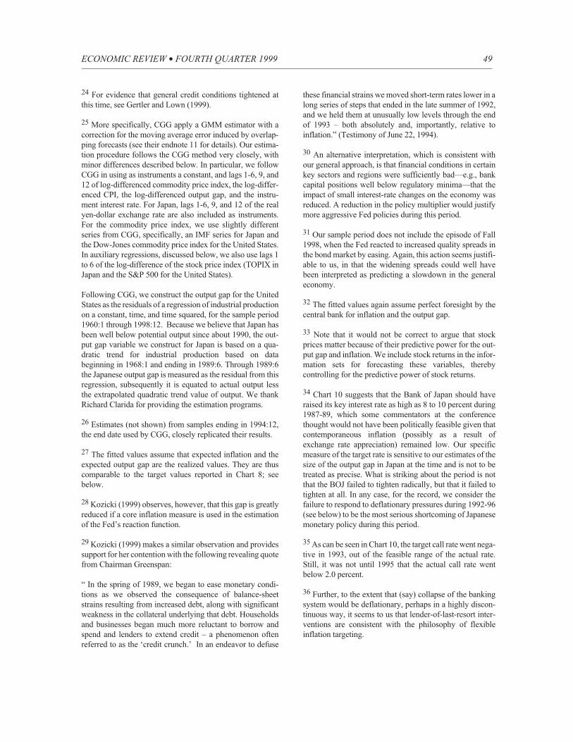
24 For evidence that general credit conditions tightened at

this time, see Gertler and Lown (1999).

25 More specifically, CGG apply a GMM estimator with a

correction for the moving average error induced by overlap-

ping forecasts (see their endnote 11 for details). Our estima-

tion procedure follows the CGG method very closely, with

minor differences described below. In particular, we follow

CGG in using as instruments a constant, and lags 1-6, 9, and

12 of log-differenced commodity price index, the log-differ-

enced CPI, the log-differenced output gap, and the instru-

ment interest rate. For Japan, lags 1-6, 9, and 12 of the real

yen-dollar exchange rate are also included as instruments.

For the commodity price index, we use slightly different

series from CGG, specifically, an IMF series for Japan and

the Dow-Jones commodity price index for the United States.

In auxiliary regressions, discussed below, we also use lags 1

to 6 of the log-difference of the stock price index (TOPIX in

Japan and the S&P 500 for the United States).

Following CGG, we construct the output gap for the United

States as the residuals of a regression of industrial production

on a constant, time, and time squared, for the sample period

1960:1 through 1998:12. Because we believe that Japan has

been well below potential output since about 1990, the out-

put gap variable we construct for Japan is based on a qua-

dratic trend for industrial production based on data

beginning in 1968:1 and ending in 1989:6. Through 1989:6

the Japanese output gap is measured as the residual from this

regression, subsequently it is equated to actual output less

the extrapolated quadratic trend value of output. We thank

Richard Clarida for providing the estimation programs.

26 Estimates (not shown) from samples ending in 1994:12,

the end date used by CGG, closely replicated their results.

27 The fitted values assume that expected inflation and the

expected output gap are the realized values. They are thus

comparable to the target values reported in Chart 8; see

below.

28 Kozicki (1999) observes, however, that this gap is greatly

reduced if a core inflation measure is used in the estimation

of the Fed’s reaction function.

29 Kozicki (1999) makes a similar observation and provides

support for her contention with the following revealing quote

from Chairman Greenspan:

“ In the spring of 1989, we began to ease monetary condi-

tions as we observed the consequence of balance-sheet

strains resulting from increased debt, along with significant

weakness in the collateral underlying that debt. Households

and businesses began much more reluctant to borrow and

spend and lenders to extend credit – a phenomenon often

referred to as the ‘credit crunch.’ In an endeavor to defuse

these financial strains we moved short-term rates lower in a

long series of steps that ended in the late summer of 1992,

and we held them at unusually low levels through the end

of 1993 – both absolutely and, importantly, relative to

inflation.” (Testimony of June 22, 1994).

30 An alternative interpretation, which is consistent with

our general approach, is that financial conditions in certain

key sectors and regions were sufficiently bad—e.g., bank

capital positions well below regulatory minima—that the

impact of small interest-rate changes on the economy was

reduced. A reduction in the policy multiplier would justify

more aggressive Fed policies during this period.

31 Our sample period does not include the episode of Fall

1998, when the Fed reacted to increased quality spreads in

the bond market by easing. Again, this action seems justifi-

able to us, in that the widening spreads could well have

been interpreted as predicting a slowdown in the general

economy.

32 The fitted values again assume perfect foresight by the

central bank for inflation and the output gap.

33 Note that it would not be correct to argue that stock

prices matter because of their predictive power for the out-

put gap and inflation. We include stock returns in the infor-

mation sets for forecasting these variables, thereby

controlling for the predictive power of stock returns.

34 Chart 10 suggests that the Bank of Japan should have

raised its key interest rate as high as 8 to 10 percent during

1987-89, which some commentators at the conference

thought would not have been politically feasible given that

contemporaneous inflation (possibly as a result of

exchange rate appreciation) remained low. Our specific

measure of the target rate is sensitive to our estimates of the

size of the output gap in Japan at the time and is not to be

treated as precise. What is striking about the period is not

that the BOJ failed to tighten radically, but that it failed to

tighten at all. In any case, for the record, we consider the

failure to respond to deflationary pressures during 1992-96

(see below) to be the most serious shortcoming of Japanese

monetary policy during this period.

35 As can be seen in Chart 10, the target call rate went nega-

tive in 1993, out of the feasible range of the actual rate.

Still, it was not until 1995 that the actual call rate went

below 2.0 percent.

36 Further, to the extent that (say) collapse of the banking

system would be deflationary, perhaps in a highly discon-

tinuous way, it seems to us that lender-of-last-resort inter-

ventions are consistent with the philosophy of flexible

inflation targeting.

ECONOMIC REVIEW l FOURTH QUARTER 1999 49

37 For an even broader indictment of fixed-exchange-rate

regimes see Obstfeld and Rogoff (1995).

38 Dollarization or a currency union represent an alternative

approach for small open economies that also avoids the

instabilities of fixed exchange rates. These approaches

have their own problems, however.

REFERENCES

Aghion, Philippe, Philippe Bacchetta, and Abhijit Banerjee.

1999. “A Simple Model of Monetary Policy and Currency

Crises,” unpublished manuscript, Massachusetts Institute

of Technology.

Allen, Franklin, and Douglas Gale. 1998. “Bubble and

Crises,” unpublished manuscript, New York University.

Bernanke, Ben S. 1983. “Non-Monetary Effects of the

Financial Crisis in the Propagation of the Great Depres-

sion,” American Economic Review, vol. 73, no. 3, June,

pp. 257-76.

Bernanke, Ben S., and Mark Gertler. 1995. “Inside the Black

Box: The Credit Channel of Monetary Transmission,”

Journal of Economic Perspectives, vol. 9, no. 4, Fall, pp.

27-48.

. 1989. “Agency Costs, Net Worth, and

Business Fluctuations,” American Economic Review, vol.

79, no. 1, March, pp. 14-31.

Bernanke, Ben S., Mark Gertler, and Simon Gilchrist. Forth-

coming. “The Financial Accelerator in a Quantitative

Business Cycle Framework,” in J. B. Taylor and M.

Woodford, eds., Handbook of Macroeconomics. Amster-

dam: North-Holland.

. 1996. “The Financial Accelerator and the

Flight to Quality,” Review of Economics and Statistics,

vol. 78, no. 1, February, pp. 1-15.

Bernanke, Ben S., and Harold James. 1991. “The Gold Stan-

dard, Deflation, and Financial Crisis in the Great Depres-

sion: An International Comparison,” in R.G. Hubbard, ed.,

Financial Markets and Financial Crises. Chicago: Uni-

versity of Chicago Press for National Bureau of Economic

Research.

Bernanke, Ben S., Thomas Laubach, Frederic S. Mishkin,

and Adam Posen. 1999. Inflation Targeting: Lessons fromthe International Experience. Princeton, N.J.: Princeton

University Press.

Bernanke, Ben S., and Cara S. Lown. 1991. “The Credit

Crunch,” Brookings Papers on Economic Activity, no. 2,

pp. 205-39.

Bernanke, Ben S., and Frederic S. Mishkin. 1997. “Inflation

Targeting: A New Framework for Monetary Policy?”

Journal of Economic Perspectives, vol. 11, no. 2, pp.

97-116.

Blanchard, Olivier, and Mark Watson. 1982. “Bubbles,

Rational Expectations, and Financial Markets,” in P.

Wachtel, ed., Crisis in the Economic and Financial Struc-ture. Lexington Books.

Bond, Stephen, and Jason Cummins. 1999. “Noisy Share

Prices and Investment,” preliminary paper, Nuffield Col-

lege and New York University, July.

Borio, C.E.V., N. Kennedy, and S.D. Prowse. 1994.

“Exploring Aggregate Asset Price Fluctuations Across

Countries: Measurement, Determinants, and Monetary

Policy Implications,” Bank for International Settlements

Economics Paper No. 40, April.

Calvo, Guillermo. 1983. “Staggered Prices in a Util-

ity-Maximizing Framework,” Journal of Monetary Eco-nomics, vol. 12, pp. 383-98.

Campbell, John. Forthcoming. “Asset Prices, Consump-

tion, and the Business Cycle,” NBER working paper no.

6485 in J. B. Taylor and M. Woodford, eds., Handbookof Macroeconomics. Amsterdam: North-Holland.

Clareida, Richard, Jordi Gali, and Mark Gertler. Forthcom-

ing. “Monetary Policy Rules and Macroeconomic Stabil-

ity: Evidence and Some Theory,” Quarterly Journal ofEconomics.

__________. 1998. “Monetary Policy Rules in Practice:

Some International Evidence,” European EconomicReview, June, pp. 1033-68.

Eichengreen, Barry. 1992. Golden Fetters: The Gold Stan-dard and the Great Depression, 1919-1939. New York:

Oxford University Press.

Eichengreen, Barry, Paul Masson, Miguel Savastano, and

Sunil Sharma. 1999. “Transition Strategies and Nominal

Anchors on the Road to Greater Exchange-Rate Flexibil-

ity,” Essays in International Finance no. 213, Interna-

tional Finance Section, Princeton University, April.

Fisher, Irving. 1933. “The Debt-Deflation Theory of Great

Depressions,” Econometrica, vol. 1, October, pp.

337-57.

Fuhrer, Jeffrey C., and George R. Moore. 1995. “Inflation

Persistence,” Quarterly Journal of Economics, vol. 110,

no. 1, February, pp. 127-60.

Hubbard, R. Glenn. 1997. “Financial Market Imperfections

and Investment,” National Bureau of Economic

Research Working Paper no. 5996, April.

Gali, Jordi, and Mark Gertler. Forthcoming. “Inflation

Dynamics: A Structural Economics Analysis,” Journalof Monetary Economics.

Gertler, Mark, and Cara S. Lown. 1999. “The Information

Content of the High Yield Bond Spread for the Business

Cycle,” unpublished manuscript, Federal Reserve Bank

of New York.

Gilchrist, Simon, and Charles Himmelberg. 1998. “Invest-

ment: Fundamentals and Finance,” in B. Bernanke and J.

Rotemberg, eds., NBER Macroeconomics Annual.Goodhart, Charles A.E., and Jose’ Viñals. 1994. “Strategy

50 FEDERAL RESERVE BANK OF KANSAS CITY

and Tactics of Monetary Policy: Examples from Europe

and the Antipodes,” in Jeffrey Fuhrer, ed., Goals, Guide-lines, and Constraints for Monetary Policymakers, Fed-

eral Reserve Bank of Boston Conference Series 38, pp.

139-87.

Haldane, Andrew G., ed. 1995. Targeting Inflation. London:

Bank of England.

Kaminsky, Graciela, and Carmen Reinhart. 1999. “The

Twin Crises: The Causes of Banking and Balance-of-Pay-

ments Problems,” American Economic Review, vol. 89,

no. 3, June, pp. 473-500.

Kiyotaki, Nobuhiro, and John Moore. 1997. “Credit

Cycles,” Journal of Political Economy, vol. 105, no. 2,

April, pp. 211-48.

Kozicki, Sharon. 1999. “How Useful Are Taylor Rules for

Monetary Policy?” Federal Reserve Bank of Kansas City,

Economic Review, Second Quarter, pp. 5-33.

Krugman, Paul. 1999. “Analytical Afterthoughts on the

Asian Crisis,” unpublished manuscript, Massachusetts

Institute of Technology.

Leiderman, Leonardo, and Lars E.O. Svensson, eds. 1995.

Inflation Targeting. London: Centre for Economic Policy

Research.

Ludvigson, Sydney, and Charles Steindel. 1999. “How

Important Is the Stock Market Effect on Consumption?”

Federal Reserve Bank of New York, Economic PolicyReview, vol. 5, no. 2, July, pp. 29-52.

Mishkin, Frederic S. 1997. “The Causes and Propagation

of Financial Instability: Lessons for Policymakers,” in

Maintaining Financial Stability in a Global Economy, a

symposium sponsored by the Federal Reserve Bank of

Kansas City, August.

Obstfeld, Maurice. 1994. “The Logic of Currency Crises,”

Banque de France, Cahiers Économiques et Monétaires,

vol. 43, pp. 189-213.

and Kenneth Rogoff. 1995. “The Mirage

of Fixed Exchange Rates,” Journal of Economic Per-spectives, vol. 9, no. 4, pp. 73-96.

Parker, Jonathan. Forthcoming. “Spendthrift in America?

On Two Decades of Decline in the U.S. Saving Rate,” in

B. Bernanke and J. Rotemberg, eds., NBER Macroeco-nomics Annual.

Svensson, Lars E.O. 1999. “Inflation Targeting as a Mone-

tary Policy Rule,” Journal of Monetary Economics, vol.

43, no. 3, June, pp. 607-54.

. 1997. “Inflation Forecast Targeting:

Implementing and Monitoring Inflation Targets,” Euro-pean Economic Review, vol. 41, pp. 1111-46.

Taylor, John B. 1993. “Discretion Versus Policy Rules in

Practice,” Carnegie-Rochester Conference Series on

Public Policy, vol. 39, pp. 195-214.

. 1980. “Aggregate Dynamics and Stag-

gered Contracts,” Journal of Political Economy, vol. 88,

pp. 1-24.

ECONOMIC REVIEW l FOURTH QUARTER 1999 51