Embed Size (px)
Citation preview

MONETARY AND FISCAL POLICY INTERACTIONS IN THEPOST-WAR U.S.
NORA TRAUM AND SHU-CHUN S. YANG
Abstract. A New Keynesian model allowing for an active monetary and passive fiscalpolicy (AMPF) regime and a passive monetary and active fiscal policy (PMAF) regime isestimated to fit various U.S. samples from 1955 to 2007. The results show that data inthe pre-Volcker periods strongly prefer an AMPF regime, even with a prior centered in thePMAF region. The estimation, however, is not very informative about whether the FederalReserve’s reaction to inflation is greater than one in the pre-Volcker period, because muchlower values can still preserve determinacy under passive fiscal policy. In addition, whethera PMAF regime can generate consumption growth following a government spending increasedepends on the degree of price stickiness. An income tax cut can yield an unusual negativelabor response if monetary policy aggressively stabilizes output growth.
Keywords: Fiscal and Monetary Policy Interactions; New Keynesian Models; Bayesian Es-timation
JEL Codes: C11; E52; E63; H30
1. Introduction
Estimated New Keynesian models often omit government debt from model specificationsand implicitly assume that lump-sum taxes adjust to clear the government budget [e.g.,Christiano, Eichenbaum, and Evans (2005) and Smets and Wouters (2003, 2007)]. Condi-tional on the existence of a unique equilibrium, this implies that monetary policy is activeand fiscal policy is passive (AMPF) in the sense of Leeper (1991).1 Economists generallyagree that monetary policy in the post-1984 U.S. has been active (characterized by an infla-tion coefficient greater than one in the Taylor rule, e.g., Taylor (1999a), Clarida, Gali, andGertler (2000), and Cogley and Sargent (2005)), implying that the monetary and fiscal policy
September 15, 2010. Department of Economics, North Carolina State University, nora [email protected];Research Department, the International Monetary Fund, [email protected]. This paper was prepared for theEuropean Economic Review Conference at Philadelphia on June 10th-11th, 2010. We thank Eric Leeper,Jesper Linde, Jim Nason, and the conference participants for helpful comments. The views expressed hereinare those of the authors and should not be attributed to the IMF, its Executive Board, or its management.
1An active authority is defined as an authority which is not constrained by current budgetary conditionsand may choose a decision rule dependent on any variables it wants. In contrast, a passive authority isconstrained by the consumers’ and firms’ optimizations and by the actions of the active authority. Thepassive authority must ensure that current budgetary conditions are satisfied, and thus, must ensure theintertemporal government budget constraint is satisfied. See Leeper (1991), Sims (1994), Cochrane (1999),and Woodford (2003) for more discussion.
1

MONETARY AND FISCAL POLICY INTERACTIONS IN THE POST-WAR U.S. 2
combination in the post-1984 U.S. fits an AMPF regime. Much uncertainty, however, existsbefore the appointment of Paul Volcker as Chairman of the Federal Reserve Board in 1979.Results from Markov-switching regressions suggest that some periods in the pre-Volcker eraare likely to be consistent with a passive monetary and active fiscal policy (PMAF) regime(Favero and Monacelli (2005), Davig and Leeper (2006), and Davig and Leeper (2009)).
This paper estimates a New Keynesian model that accounts for monetary and fiscal policyinteractions with Bayesian methods. Differing from most estimated New Keynesian models,our specification features government debt and fiscal financing, which is necessary to allowfor the possibility of a PMAF regime. We estimate the model imposing an AMPF or aPMAF regime over three samples—1955Q1-1966Q4, 1967Q1-1979Q2, and 1984Q1-2007Q4.For all the samples investigated, estimations are conducted under three specifications. Thefirst two have priors centered at an AMPF regime and a PMAF regime respectively, butallow for parameter combinations to be in the parameter space of both regions. The thirdspecification imposes a PMAF regime by not allowing fiscal instruments to respond to debtgrowth.
Except for the third specification imposing the PMAF regime, the posterior distributionsfall in the parameter space of the AMPF regime, regardless of the prior. Model comparisonsindicate that for all three samples, the data prefer least the specification with a PMAF regimeimposed. Moreover, competing estimates for the Federal Reserve’s response to inflation arefound in the pre-Volcker period within the parameter space of an AMPF regime: one wherethe inflation coefficient is larger than one—when the prior for this variable is larger thanone as in the first specification, and one where it is smaller than one—when the prior ismuch below one as in the second specification. Although the conventional boundary of themonetary authority’s response to inflation for active monetary policy is (near) one,2 theboundary can be much below one in medium and large scale New Keynesian models. Theresult suggests that the estimates from New Keynesian models for the pre-Volcker sample arelikely to be influenced by priors. Hence, the conclusion reached by estimated New Keynesianmodels about whether the monetary authority’s response to inflation was sufficient in thepre-Volcker period may be driven to a large extent by the prior imposed.3
The distinctive difference in the macroeconomic dynamics in the pre- and post-Volcker pe-riods, particularly in inflation, has spurred tremendous interests in search for explanations.The increasing macroeconomic stability in the post-Volcker period has been attributed to“Good Luck” or “Good Policy.” The “Good Luck” theory argues that the Federal Reserve’sresponse to inflation was sufficient in the pre-Volcker period and attribute the reduced eco-nomic instability in the post-Volcker period to the reduced variance of structural disturbances(Canova and Gambetti (2009), Sims and Zha (2006), and Primiceri (2005)). On the otherhand, the “Good Policy” theory attributes the persistent high inflation in the pre-Volckerperiod to the Federal Reserve’s insufficient abilities to control inflation. These conclusionsare often based on the inflation coefficient in a Taylor-type rule being estimated as smallerthan one (e.g., Judd and Rudebusch (1998), Taylor (1999b), Cogley and Sargent (2005), and
2See Leeper (1991), Sims (1994), and Woodford (2003).3Smets and Wouters (2007) obtain the mode for the inflation coefficient in the monetary policy rule 1.65
for the 1966Q1-1979Q2 sample under the prior mean of 1.5.

MONETARY AND FISCAL POLICY INTERACTIONS IN THE POST-WAR U.S. 3
Boivin (2006)).4 When analyzing the implication of a passive monetary policy rule in a NewKeynesian model, several papers further conclude that monetary policy in the pre-Volckerperiod implies indeterminacy of the equilibrium, and that the high volatility in inflation andoutput during the period could be due to sunspot fluctuations (Clarida, Gali, and Gertler(2000), Lubik and Schorfheide (2004), and Boivin and Giannoni (2006)). Instead, whenallowing for regime switches in monetary policy, Davig and Leeper (2006), Davig and Doh(2009), and Bianchi (2010) conclude that monetary policy was passive (and determinate) attimes in the pre-Volcker era.
This paper contributes to this literature by estimating AMPF and PMAF regimes in thepre- and post-Volcker periods and evaluating their relative fit. As noted in ?, many differentmonetary and fiscal policy combinations result in the same stochastic processes for variablesin a model, posing an identification challenge. The approach in this paper is to estimate aDSGE model with fixed policy rules that deliver an AMPF or PMAF solution, dependingupon the monetary and fiscal policy parameters. The specificity of the policy rules imposesidentification restrictions that allow us to identify the AMPF and PMAF regimes.
We find that the PMAF regime is never favored by the data due to the high volatility thefixed PMAF regime implies for certain observables, particularly hours worked and inflation.The results suggest that the standard New Keynesian model used for policy analysis isnot able to match features of the data if a fixed PMAF regime is assumed.5 In addition,substantial changes in the structural innovations in the pre- and post-Volcker periods arefound. Contrary to the conclusions from VAR evidence, we do not find reduced monetarypolicy effects on output in the post-Volcker period (Gertler and Lown (1999), Barth andRamey (2002), and Boivin and Giannoni (2002)).
Another finding of the paper is that a PMAF regime can generate a positive consumptionresponse to an increase in government spending, but the degree of price stickiness is crucialto deliver the result. Kim (2003) and Davig and Leeper (2009) demonstrate that a PMAFregime can yield a positive consumption response following a government spending shock,due to a reduction in the real interest rate. Under the imposed PMAF regime (the thirdspecification), a positive consumption response following a government spending increase isfound for 1967Q1-1979Q2, but the consumption response is almost negligible for 1955Q1-1966Q4. Because the estimated degree of price stickiness for 1955Q1-1966Q4 is quite high, agovernment spending increase leads to a small and slow increase in the price level and doesnot lower the real interest rate.
Finally, the paper demonstrates that policy coordination is important for the expansion-ary effect of a tax cut. When the monetary authority reacts relatively weakly to inflationand strongly to output growth induced by a tax cut, labor can fall and thus dampen thestimulative effect of the tax cut. A monetary tightening triggers asset substitution betweengovernment bonds and physical capital and thus offsets the investment incentive from a lowerincome tax rate. As investment is dampened, firms’ demand for labor also weakens. Despite
4Also see Romer and Romer (2002) and Meltzer (2005) for narrative evidence supporting the view thatmonetary policy was passive in the 1970s. Based upon the real-time estimates of the output gap, Orphanides(2003), however, argues that the Federal Reserve’s response to inflation was sufficient in controlling inflation.
5Caivano (2007) reaches a similar conclusion that the fiscal theory of price determination (embedded inthe PMAF regime) cannot explain the high inflation in the U.S. from 1968 to 1979 by fitting a stylized NewKeynesian model.

MONETARY AND FISCAL POLICY INTERACTIONS IN THE POST-WAR U.S. 4
the households’ desires to increase labor supply given a lower income tax rate, equilibriumlabor falls, and the expansionary effect from an income tax cut is diminished.
2. Model
We estimate a standard New Keynesian model that includes a stochastic growth path,as in Del Negro, Schorfheide, Smets, and Wouters (2007) and ?. Differing from most NewKeynesian models with a focus on monetary policy, our model also emphasizes fiscal behavior,which allows for the interactions between monetary and fiscal policy.
2.1. Firms. The production sector consists of intermediate and final goods producing firms.A perfectly competitive final goods producer uses a continuum of intermediate goods yt(i),where i ∈ [0, 1], to produce the final goods, Yt, according to the constant-return-to-scaletechnology due to Dixit and Stiglitz (1977),
[∫ 1
0
yt(i)1
1+ηpt di
]1+ηpt
≥ Yt , (1)
where ηpt denotes an exogenous time-varying markup to the intermediate goods’ prices.
Denote the price of the intermediate goods i as pt(i) and the price of final goods Yt asPt. The final goods producing firm chooses Yt and yt(i) to maximize profits subject to thetechnology (1). The demand for yt(i) is given by
yt(i) = Yt
(
pt(i)
Pt
)
−1+η
pt
ηpt
, (2)
where1+ηp
t
ηpt
is the elasticity of substitution between intermediate goods.
Intermediate goods producers are monopolistic competitors in their product market. Firmi produces by a Cobb-Douglas technology
yt(i) = A1−αt kt(i)
αLt(i)1−α , (3)
where α ∈ [0, 1]. Fixed costs of production are assumed to be zero, as in ?. At denotes apermanent shock to technology. Its growth rate, at = lnAt − lnAt−1, follows a stationaryAR(1) process,
at = (1 − ρa)γ + ρaat−1 + ǫat , ǫat ∼ i.i.d. N(0, σ2
a) , (4)
where γ is the steady-state growth rate.
The price rigidity of the model is introduced by a Calvo (1983) mechanism. An interme-diate firm has a probability of (1 − ωp) each period to reoptimize its price to maximize theexpected sum of discounted future real profits. Those cannot do so index their prices to pastinflation according to the rule
pt(i) = pt−1(i)πχp
t−1π1−χp
. (5)

MONETARY AND FISCAL POLICY INTERACTIONS IN THE POST-WAR U.S. 5
2.2. Labor Packers. A perfectly competitive labor packer purchases a continuum of dif-ferentiated labor inputs Lt(j), where j ∈ [0, 1], from the households and assembles them toproduce a composite labor service Lt (sold to intermediate goods producing firms) by thetechnology,
Lt =
[∫ 1
0
Lt (j)1
1+ηwt dj
]1+ηwt
, (6)
where ηwt denotes a time-varying exogenous markup to wages.
The demand function for a labor packer is
Lt (j) = Lt
(
Wt(j)
Wt
)
−1+ηw
tηwt
, (7)
where Wt(j) is the wage received from the labor packer by the household j, and Wt is thewage for the composite labor service paid by intermediate firms.
2.3. Households. Each household j maximizes its utility, given by
Et
∞∑
s=0
βsubt+s
[
ln(ct+s − θCt+s−1) −ϕLt+s(j)
1+ν
1 + ν
]
, (8)
where β ∈ (0, 1) is the discount factor, θ ∈ (0, 1) is external habit formation, ν ≥ 0 isthe inverse of the Frisch labor elasticity, and ϕ is the disutility weight on labor. Eachhousehold owns one unique labor input Lt(j) and is the wage setter for that input, asin Erceg, Henderson, and Levin (2000). Due to the existence of state-contingent claims,consumption ct and asset holdings are the same for all households and thus are not indexedby j. ubt is a shock to general preferences that follows the AR(1) process,
ln ubt = (1 − ρb) ln ub + ρb ln ubt−1 + ǫbt , ǫbt ∼ i.i.d. N(0, σ2b ) . (9)
The household j’s flow budget constraint in units of consumption goods is
ct + it + bt + ςt+1,txt(j) =
(1 − τt)Wt(j)Lt(j) + (1 − τt)RKt vtkt−1 − ψ(vt)kt−1 +
Rt−1bt−1 + xt−1(j)
πt+ Zt +Dt , (10)
where τt is the income tax rate.6 Asset holding consists of the accumulation of gross in-vestment it for capital stock kt, one period risk-free government bonds bt, and household j’snet acquisition of state contingent claims xt(j). Each household owns an equal share of allintermediate firms and receives the share Dt of intermediate firms’ profits. In addition, eachhousehold receives a lump-sum transfer Zt from the government.
Households control both the size of the capital stock and its utilization rate vt. Effectivecapital, kt = vtkt−1 is rented to firms at the rate Rk
t . The cost of capital utilization is ψ(vt)
6Our modeling choice of a single income tax rate and tax-exempt government bonds is driven by twoconsiderations. First, we intend to reduce the size of the system estimated. To model separately labortaxes, capital taxes, and interest income taxes on government bonds would require adding two additionaltax variables in the observables. Second, while labor and capital income taxes have different effects, for thepurpose of characterizing active and passive fiscal policy, they serve the same financing role to stabilize debtgrowth.

MONETARY AND FISCAL POLICY INTERACTIONS IN THE POST-WAR U.S. 6
per unit of physical capital. In the steady state, v = 1 and ψ(1) = 0. Define a parameter
ψ ∈ [0, 1) such that ψ′′(1)
ψ′ (1)
≡ ψ
1−ψ. Then, the law of motion for private capital is
kt = (1 − δ)kt−1 + uit
[
1 − s
(
itit−1
)]
it , (11)
where s(
itit−1
)
× it is an investment adjustment cost, as in Smets and Wouters (2003) and
Christiano, Eichenbaum, and Evans (2005). By assumption, s(γ) = s′ (γ) = 0, and s′′ (γ) ≡s > 0. uit captures exogenous variations in the efficiency with which investment can betransformed into physical capital, as in Greenwood, Hercowitz, and Krusell (1997). It evolvesaccording to
ln uit = (1 − ρi) lnui + ρi ln uit−1 + ǫit, ǫit ∼ i.i.d. N(0, σ2i ) . (12)
Each period a fraction (1 − ωw) of households are allowed to re-optimize their nominalwage rate by maximizing
Et
∞∑
s=0
βsωsw
[
−ubt+sϕLt(j)
1+ν
1 + ν
]
, (13)
subject to their budget constraint (10) and the labor demand function (7). The fraction ωwof households that cannot re-optimize index their wages to past inflation by the rule
Wt (j) = Wt−1 (j) (πt−1eat−1)χ
w−1(πeγ)1−χw
. (14)
2.4. Monetary Policy. The monetary authority follows a Taylor-type rule, in which thenominal interest rate Rt responds to its lagged value, the current inflation rate, and currentoutput. Denote a variable in percentage deviations from the steady state by a caret, as inRt. Specifically, the interest rate is set by
Rt = ρrRt−1 + (1 − ρr)(
φππt + φyYt
)
+ ǫrt , ǫrt ∼ N(0, σ2r ) . (15)
2.5. Fiscal Policy. Each period the government collects tax revenues and issues one-periodnominal bonds to finance its interest payments and expenditures, which include governmentconsumption Gt and transfer payments to the households. Denote aggregate effective capitaland bonds by Kt and Bt. The flow budget constraint in units of consumption goods is
Bt + τt(RktKt +WtLt) =
Rt−1Bt−1
πt+Gt + Zt . (16)
Fiscal variables respond to the lagged debt-to-output ratio according to the following rules:
τt = ρτ τt−1 + (1 − ρτ )γτ sbt−1 + ǫτt , ǫτt ∼ i.i.d. N(0, σ2
τ ) , (17)
Gt = ρgGt−1 − (1 − ρg)γgsbt−1 + ǫgt , ǫgt ∼ i.i.d. N(0, σ2
g) , (18)
andZt = ρzZt−1 + ǫzt , ǫzt ∼ i.i.d. N(0, σ2
z) , (19)
where sbt−1 ≡Bt−1
Yt−1. Transfers are non-distortionary and are simply modeled as a residual in
the government budget constraint, exogenously determined by an AR(1) process. Becauseour data set does not include transfers, Zt can be thought of as capturing all movements in

MONETARY AND FISCAL POLICY INTERACTIONS IN THE POST-WAR U.S. 7
government debt that are not explained by the model or the government spending and taxshocks.7
Denote aggregate quantities by capital letters. The goods market clearing condition is
Ct + It +Gt + ψ(vt)Kt−1 = Yt . (20)
2.6. Model Solution. The equilibrium consists of optimality conditions for the households’and firms’ optimization problems, market clearing conditions, the government budget con-straint, monetary and fiscal policy rules, and the stochastic processes for all shocks. Becausethe model features stochastic growth, some level variables are transformed by the technologylevel At to gain stationarity. The equilibrium system is log-linearized around the steady stateof the transformed model and solved by Sims’s (2001) algorithm. Appendix A describes thestationary equilibrium, the steady state, and the log-linearized system.
There are two distinct regions of the parameter subspace that deliver a unique rationalexpectations equilibrium—an active monetary, passive fiscal policy (AMPF) regime or apassive monetary, active fiscal (PMAF) policy regime. In the AMPF regime, the monetaryauthority responds to inflation deviations from its target level sufficiently to stabilize the in-flation path, while the fiscal authority adjusts government spending or tax policy to stabilizegovernment debt growth. In the PMAF regime, the fiscal authority does not take sufficientmeasures to stabilize debt; instead, the monetary authority pursues actions to stabilize debtgrowth through price adjustments. We consider both of these regimes in the analysis thatfollows.
3. Estimation
The model is estimated with quarterly data for three samples in the post-war U.S.:1955Q1-1966Q4, 1967Q1-1979Q2, and 1984Q1-2007Q4. The first sample has been shownto be consistent with a passive monetary policy and active fiscal policy regime (Davig andLeeper (2006) and Davig and Leeper (2009)). The remaining two samples correspond tothe “Great Inflation” and “Great Moderation,” as recognized by the literature. The GreatInflation featured a period of rapid inflation growth and persistent, high inflation. It endedwith the appointment of Paul Volcker as Chairman of the Federal Reserve Board in August1979. The Great Moderation featured stable, low inflation and reduced volatility in macroe-conomic aggregates. It lasted until the beginning of the worst and longest recession in thepost-WW2 history in December 2007.
Nine observables are used for the estimation, including real consumption, investment,wages, government spending, tax revenue, government debt, hours worked, inflation, andthe federal funds rate.8 Data for the observables and the log-linearized variables are linked
7One common specification in modeling income taxes is to include an automatic stabilizing component.Initial estimations find that the data we use are not informative about the parameter for contemporaneousoutput in (17). Thus, our analysis does not focus on the automatic stabilizing role of income taxes.
8As pointed out by Schmitt-Grohe and Uribe (2010), without including the relative price of investmentgoods in observables, it is likely to obtain a counterfactually large estimate for the standard deviation forthe investment efficiency shock. Also, because the paper focuses on feedbacks from debt to distorting fiscalvariables, it is essential to include a measure of government debt in the observables. We found that using

MONETARY AND FISCAL POLICY INTERACTIONS IN THE POST-WAR U.S. 8
by the following equations:
dlConstdlInvt
dlWagetdlGovSpendtdlTaxRevtdlGovDebtt
lHoustlInflt
lFedFundst
=
100γ100γ100γ100γ100γ100γ
000
+
ct − ct−1 + atit − it−1 + atwt − wt−1 + atgt − gt−1 + attt − tt−1 + atbt − bt−1 + at
LtπtRt
, (21)
where l and dl stand for 100 times the log and the log difference of each variable. Smallletters denote the transformed quantity of a level variable. tt is transformed tax revenue, andat is the percentage deviation of the technology growth rate from the steady-state growthrate γ. The analysis focuses on the fiscal behaviors of the federal government; thus, fiscaldata do not include those for state and local governments. Appendix B provides a detaileddescription of the data.
3.1. Methodology. We assume that the parameters are drawn independently, and let p(θ)be the product of the marginal parameter distributions. Given the plausible interactionsbetween monetary and fiscal policies, p(θ) has a non-zero density outside the determinacyregion of the parameter space. The analysis is restricted to the parameter subspace thatdelivers a unique rational expectations equilibrium—i.e. an AMPF regime or a PMAFpolicy regime. Denote this subspace as ΘD, and let I{θ ∈ ΘD} be an indicator function thatis one if θ is in the determinacy region and zero otherwise. Then, the joint prior distributionis defined as
p(θ) =1
cp(θ)I{θ ∈ ΘD}, where c =
∫
θ∈ΘD
p(θ)dθ .
The equilibrium system is written in a state-space form, where observables are linked withother variables in the model. For a given set of structural parameters, the value for the logposterior function is computed. The minimization routine csminwel by Christopher Sims isused to search for a local minimum of the negative log posterior function.9
The posterior distribution is constructed using the random walk Metropolis-Hastings al-gorithm. In each estimation, we sample 2.02 million draws from the posterior distributionand discard the first 20,000 draws. The sample is thinned by every 25 draws, which leavesa final sample size of 80,000. A step size of 0.33 yields an acceptance ratio from 0.27 to0.33 across estimations. Diagnostic tests are performed to ensure the convergence of theMCMC chain, including drawing trace plots, verifying whether the chain is well mixed, andperforming Geweke’s ((2005), pp. 149-150) Separated Partial Means test.
either government debt growth or the debt-to-GDP ratio as an observable made little difference for posteriorestimates. Results are available in the Estimation Appendix.
9To search for the posterior mode, we first calculate the posterior likelihood at 5000 initial draws. The 50draws with the highest posterior likelihood are used to initialize the search. The mode search that delivers thelowest negative log posterior value is used as the local mode to initialize the random walk Metropolis-Hastingsalgorithm.

MONETARY AND FISCAL POLICY INTERACTIONS IN THE POST-WAR U.S. 9
3.2. Prior Distributions. Several parameters that are hard to identify from the data arecalibrated. The discount factor, β, is set to 0.99. The capital income share of total output,α, is set to 0.3, implying a labor income share of 0.7. The quarterly depreciation rate forcapital, δ, is set to 0.025, implying the annual depreciation rate is 10 percent. ηw and ηp
are set to 0.14, so that the steady-state markups in the product and labor markets are 14percent.
The steady-state fiscal variables are also calibrated to the mean values of our data from1955Q1 to 2007Q4.10 The tax rate, the ratio of government spending to output, and theratio of government debt to annual output are set to 0.185, 0.104, and 0.348, respectively.When computing these statistics from the data, output is defined as the sum of consump-tion, investment, and government consumption and investment, consistent with the outputdefinition in the model.
For each sample, the model is estimated with three different priors, given under the priorcolumn in Tables 1, 2, and 3. The only difference amongst the priors is the priors for themonetary and fiscal policy parameters: φπ, γg, and γt. The specifications assign differentweights to the AMPF and PMAF regimes. The first prior specification, P1, is centered at theAMPF regime. The inflation and output coefficients (φπ and φy) follow the common priorsadopted in the literature for U.S. data; the monetary authority raises the interest rate bymore than the inflation rate to combat inflation deviations from its target (e.g., Smets andWouters (2007), Del Negro, Schorfheide, Smets, and Wouters (2007)). The fiscal authorityadjusts government spending and the tax rate to stabilize the debt growth relative to thesize of output. We assume normal distributions for the responses of fiscal instruments todebt (γg and γt) with a mean of 0.15 and a standard deviation 0.05, similar to those used inTraum and Yang (2010).
The second prior specification, P2, is centered at the PMAF regime. In this specification,the monetary authority raises the interest rate less than one-for-one with inflation deviations,and the fiscal authority does not adjust instruments sufficiently to control debt growth. φπhas a beta distribution with a mean of 0.5 and a standard deviation of 0.2, and γg and γtboth have normal distributions with zero means and standard deviations of 0.03. The thirdprior specification, P3, is restricted to the PMAF regime, and assumes the fiscal authoritycannot use the fiscal instruments to control debt growth. φπ has a beta distribution with amean of 0.5 and a standard deviation of 0.2, as in P2.
A priori, we do not have a view about how policy regimes influence the structural pa-rameters. Thus, our priors for all other estimated parameters follow closely those of Smetsand Wouters (2007) and Justiniano, Primiceri, and Tambalotti (2010). The prior for thepercentage growth rate of technology (100γ) is normally distributed with a mean of 0.5and a standard deviation of 0.03. The tight prior is meant to guide the estimate to matchthe average quarterly growth rate of real output (the sum of consumption, investment, andgovernment consumption and investment) per capita, which is 0.47 from 1955Q1 to 2007Q4.
10Whether the steady-state fiscal values are calibrated to sub-sample means or the means of the entiresample makes little difference for the estimation (see the Estimation Appendix for more details). Calibratingsteady-state fiscal variables to the average of a longer horizon implies that the fiscal authority may not raisetaxes or cut spending when the debt-to-output ratio is temporarily higher than the sub-sample mean butlower than the mean of the entire sample.
MONETARY AND FISCAL POLICY INTERACTIONS IN THE POST-WAR U.S. 10
Given the complexity of the model, the parameter space for policy regimes cannot be char-acterized analytically. Instead, a numerical approach is used to search for the boundaries ofthe parameter space that yield an AMPF or a PMAF regime. For a parameter combinationthat delivers a determinate equilibrium, we further check whether the determinacy can bepreserved if the fiscal policy specification is replaced with one where transfers adjust suffi-ciently to stabilize debt growth—a definite passive fiscal policy. In this case, γg = γt = 0, thecoefficient of transfers’ response to debt is set to 0.5, and other parameters are held at theiroriginal values. If a determinate equilibrium is found under this passive fiscal policy, thenthe original parameter combination implies an active monetary policy.11 The same approachis used to examine the policy regimes implied by parameter combinations drawn from thethree prior specifications. The probabilities for the PMAF regime under P1, P2, and P3specifications are 1.15, 99.97, and 100 percent, respectively.
Figure 1 plots combinations of various parameters and the monetary authority’s responseto inflation, φπ, that deliver the AMPF regime. For each plot, all other parameters are heldat their mean values in the P1 specification. Although the boundary condition for φπ occursaround one for most parameter combinations, the plots show that the values of ωp, ωw,φy, and ρr influence the boundary value of φπ. This finding is consistent with the results ofFlaschel, Franke, and Proano (2008). Values of φπ much smaller than one are consistent withactive monetary policy when wages and/or prices are very sticky. For instance, φπ ≥ 0.7 isconsistent with an AMPF regime when ωw = 0.9 (and all other parameters are kept at theirprior means). High price stickiness implies that current and future prices adjust very slowly.In this case, the monetary authority need not respond more than one-for-one to inflation,provided it responds to output, as expectations of future inflation deviations are alreadysmall. Similarly, very sticky nominal wages translate into smaller inflation deviations andinflation expectations, because the marginal cost of the intermediate goods producing firmsand, in turn, the general price level are driven by factor prices.
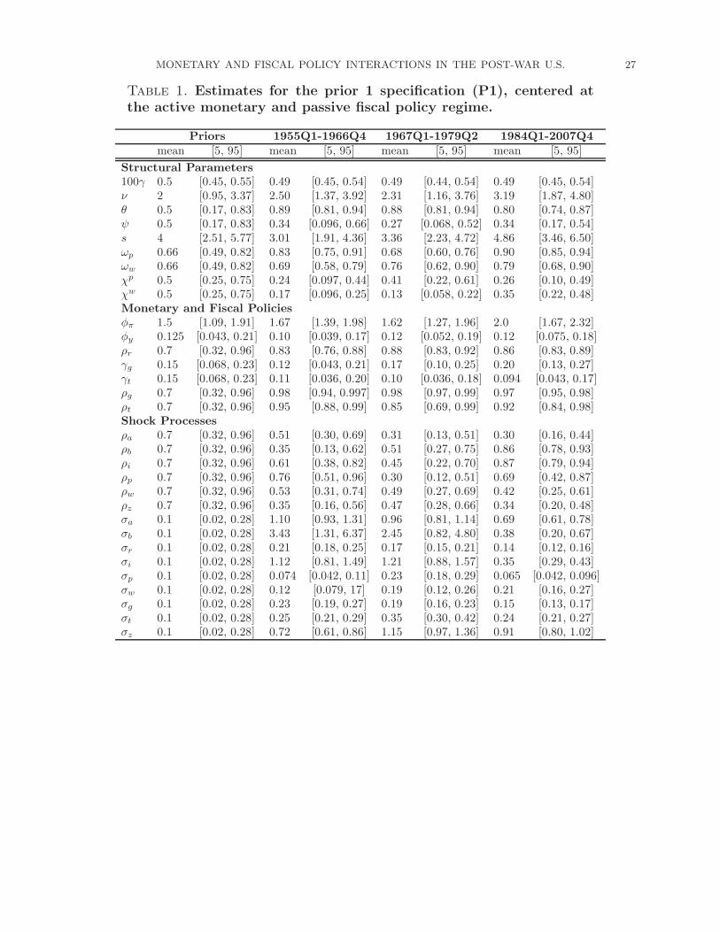
3.3. Posterior Estimates. Tables 1, 2, and 3 compare the means and 90-percent credibleintervals of the posterior distributions estimated from the three prior specifications acrossall the sample periods. Overall the data are informative about most of the parameters,as the 90-percent credible intervals for most of the parameters are different from thoseimplied by the prior distributions. The sole exception is the technology growth rate γ,whose posterior estimate closely mimics its prior. Our estimates for structural parametersare similar to previous estimates from similar DSGE models (e.g., Smets and Wouters (2007)and Del Negro, Schorfheide, Smets, and Wouters (2007)).
Several observations can be made when comparing the estimates across the sample periods.Conditional on a sample period, the prior specifications only have a small influence on theestimates of most non-policy parameters. The exceptions are the degrees of price and wagestickiness (ωp and ωw), which have higher estimates from the P2 and P3 specifications thanthe typical estimates in the literature. In Section 4, we investigate further why nominal
11To ensure our approach is robust, the exercise is also conducted from the opposite direction. We alsocheck if a determinate equilibrium can be found when an active fiscal policy is imposed (by not allowingany fiscal variables respond to debt), which implies the original parameter combination has a PMAF regime.The results show that checking from either direction yield the same conclusion in determining the policyregime of a parameter combination.
MONETARY AND FISCAL POLICY INTERACTIONS IN THE POST-WAR U.S. 11
rigidities have high estimates under P2 and P3. Both government spending and taxes areconsistently used to finance debt, as the 90-percent credible intervals for γg and γt arepositive in all samples of the P1 and P2 specification, except the estimate for γg for 1955Q1-1966Q4 under P2. In addition, adjustments in government spending are increasingly madeacross samples to finance debt. The volatility of several shocks, including the monetarypolicy shock, decreases over time. However, the largest magnitude reduction in the standarddeviation of the monetary policy shocks—from 0.17 in the 1967Q1-1979Q2 sample to 0.14 inthe 1984Q1-2007Q4 sample under P1—is smaller than those found in the literature.12 Thevolatility of the tax and transfer shocks is the highest in 1967Q1-1979Q2, allowing the modelto match the increase in the standard deviation of government debt growth over this period(see Table 4).
Our estimated response of the interest rate to inflation, φπ, for the two pre-Volcker samplesunder the standard prior specification (P1) is substantially higher than several previousestimates (Clarida, Gali, and Gertler (2000), Cogley and Sargent (2005), Boivin (2006) andBilbiie, Meier, and Muller (2008)), but are comparable to those from Bayesian estimationsof DSGE models (see Smets and Wouters (2007) and Arestis, Chortareas, and Tsoukalas(2010)). Low values of φπ are often thought to be necessary to match the persistence andvolatility of inflation in the Great Inflation era. Consistent with this view, most of ourestimates for φπ are lower in the two pre-Volcker samples than the Great Moderation era,but the model still tends to overestimate the volatility of inflation (see Table 4). Because ofthe need to match the large variances of government debt growth and tax revenue growth inthe data and the fact that distortionary financing of government debt increases the volatilityin the model, our model setup, which is a rather standard New Keynesian model, cannotquite reconcile its estimated variances of inflation and the nominal interest rate with thedata counterpart.13 This suggests that further research is needed in exploring alternativemodel specifications to better capture the observed variances among various monetary andfiscal variables.
Finally, our estimated response of the interest rate to output is also somewhat high.The interest rate’s response to output (φy) in the post-Volcker sample under P1 is closeto the standard Taylor-rule value of 0.5 (based on the annualized interest rate) from asingle-equation estimation but higher than those obtained from structural estimations. Ourmean estimate of φy is 0.12 in the 1984Q1-2007Q4 sample under P1, much higher than 0.08obtained by Smets and Wouters (2007) for a similar sample period. Also, using the methodof minimum distance estimation, Boivin and Giannoni (2006) obtain almost zero responsesof the interest rate to output deviations for both the pre- and post-Volcker samples.
12Boivin and Giannoni (2006) find that the standard deviation of the interest rate is 0.48 for the 1959Q1-1979Q2 sample and 0.23 for the 1979Q3-2002Q2 sample. Smets and Wouters (2007) report that the estimatedmode for the standard deviation of the monetary policy shock falls from 0.2 in the 1966Q1-1979Q2 sampleto 0.12 in the 1984Q1-2007Q4 sample.
13In contrast, Justiniano, Primiceri, and Tambalotti (2010) slightly underpredict this volatility over theperiod 1954Q3-2004Q4 using a similar model specification without fiscal policy and fiscal observables.

MONETARY AND FISCAL POLICY INTERACTIONS IN THE POST-WAR U.S. 12
4. Regime Analysis
Given that the different prior specifications force the model into the AMPF or PMAFregimes, we perform posterior odds comparisons to determine which regime is favored by thedata. Bayes factors are used to evaluate the relative model fit for the three samples. Table5 presents the results. Bayes factors are based on log-marginal data densities calculatedusing Geweke’s (1999) modified harmonic mean estimator with a truncation parameter of0.5. Across all three samples, the data prefer the P1 specification, although the evidencefavoring P1 over P2 for 1955Q1-1966Q4 and 1967Q1-1979Q2 is weak.14 Consistent withexpectations, the P1 specification performs much better than the alternative specificationsfor the 1984Q1-2007Q4 sample. All samples strongly dislike the P3 specification.
The P2 and P3 specifications have a harder time than the P1 specification matching vari-ous unconditional moments of the observables. When the monetary authority responds lessthan one-for-one with inflation deviations, the model specification implies a high volatility inprices, the nominal interest rate, and hours worked. This can be seen from the unconditionalmean and 90-percent credible interval from the prior distributions of the observables’ stan-dard deviations (see Table 6). Given that the fiscal authority does not respond sufficientlyto maintain budget solvency under P2 and P3 and that the model only features one-quarter,short-term government bonds, prices must adjust sufficiently within the quarter to stabilizethe real value of government indebtedness.
In estimation, to reconcile the volatile inflation implied by the P2 and P3 priors and themuch smoother inflation series in the data, the posterior forces the estimated price and wagestickiness to be high, much higher than the common estimated values observed under P1 or inthe literature. High degrees of nominal stickiness imply slow price adjustments that dampenthe volatility of inflation, allowing the model to better match the data. Figure 2 plots priorand posterior bivariate densities of the unconditional standard deviation of inflation and theCalvo pricing parameter ωp under the P2 and P3 specifications estimated from the 1955Q1-1966Q4 sample. Unlike the priors, the posterior densities give high weight exclusively to largedegrees of price stickiness. Similar changes from prior to posterior densities are also observedwhen plotting bivariate densities of the unconditional standard deviation (covariance) ofinflation or (and) the nominal interest rate against one of the two Calvo parameters—ωp orωw—across all samples estimated.
It may seem puzzling that the P2 specification is preferred to P3, given that the priorsare very similar. However, the estimates from these two specifications assign quite differentweights to the policy regimes. The posterior draws under P3 are entirely concentrated inthe PMAF regime (by design), while the posterior draws under P2 are almost exclusivelylocated in the AMPF regime, despite that the P2 prior gives substantial weight to the PMAFregion (with 99.97 percent probability in the PMAF regime). Specifically, 99.95, 99.85, and100 percent of the posterior draws under P2 are located in the AMPF region for 1955Q1-1966Q4, 1967Q1-1979Q2, and 1984Q1-2007Q4 respectively.
The difference in regime estimates by the P2 and P3 specifications has important conse-quences for the estimated volatility of the model. Table 4 gives the unconditional mean and
14The results from the priors centered at the PMAF regime (P2 and P3) may be penalized by the highposterior estimates for the degrees of price and wage stickiness, which are outliers from their priors.

MONETARY AND FISCAL POLICY INTERACTIONS IN THE POST-WAR U.S. 13
90-percent credible interval from the posterior distribution of the observables’ standard devi-ations for the various specifications. It also lists the standard deviations calculated from thedata. In all samples, the P3 estimates substantially increase the volatility of hours workedand the covariance of hours worked with other variables (not presented)—much higher thanthe data counterpart. In contrast, the P2 estimates match the statistics from the data muchbetter, which explains why P2 is preferred in model comparisons.
What accounts for the volatility to hours worked? Given that prices and/or wages areestimated to be very sticky, wages are slow to adjust. Slower wage adjustments induce morechanges in firms’ labor demand following structural and policy shocks, which drives up thevariance of hours worked. Although this effect occurs in both the P2 and P3 specifications,the effect is much stronger in the P3 specification due to different monetary policy estimates.The estimated response of the interest rate to output, φy, under P2 is approximately doublethe one under P3. The P2 specification allows the monetary authority to respond moreaggressively to output fluctuations, dampening the effects of expansions or contractions inthe economy. As a result, firms do not adjust their labor demand as much following shocksunder P2 compared to under P3, where the monetary authority responds weakly to outputfluctuations. Figure 3 illustrates this by plotting prior and posterior bivariate densities ofthe unconditional standard deviation of labor and the interest rate response to output φyfor the P2 and P3 specifications estimated from 1955Q1-1966Q4.
The difference in monetary policy estimates across P2 and P3 (specifically φy) is explainedby the different policy regimes implied by the prior and the posterior under P2. As we haveseen, the P2 specification implies a very high estimated degree of nominal stickiness and alarge interest rate response to output deviations. Both of these features help simultaneouslydampen inflation and hours worked volatility. Thus, the interest rate’s response to inflationneed not be larger than one in order to sufficiently stabilize inflation. Monetary policy forthe vast majority of draws from the posterior distribution under P2 is active despite that themean estimate of φπ is centered at values much below one for all three samples (see Table2). On the other hand, under P3, while the posterior estimations also push the estimatesfor nominal rigidities to be high to reduce the price and interest rate volatilities, the fixedPMAF regime forces the interest rate response to inflation to be low (with the mean estimatefrom 0.23 to 0.4 across sample, see Table 3) in order to maintain passive monetary policy.Thus, the estimation under P3 does not have sufficient degree of freedom among parametersto reduce volatility of inflation and hours worked to be more in line with the data. It is notsurprising that the model fit to data under P3 is the worst among the three specifications.
The analysis here suggests that although the model comparisons indicate that the dataacross all three samples prefer the P1 specification (where the posterior falls in the AMPFregime and the monetary authority’s response to inflation is much higher than one), itis unclear whether our conclusion about policy regimes, particularly for the pre-Volckersamples, would hold in a more general model of monetary and fiscal policy interactions.Echoing the implication in Section 3 regarding the over-estimated variances of inflation andthe nominal interest rate, our results suggest that the standard New Keynesian model usedfor policy analysis is not able to match features of the data if a PMAF regime is assumed.One possible future generalization that may reduce the inflation volatility of the PMAFregime is a model that includes longer maturity horizons for government debt.
MONETARY AND FISCAL POLICY INTERACTIONS IN THE POST-WAR U.S. 14
5. Applications
In this section, we use the estimated model to study monetary and fiscal policy effects.Three applications are investigated: the evolution of monetary policy effects in the post-war U.S., the effect of a government spending increase under a PMAF regime, and theexpansionary effect of an income tax cut.
5.1. The Evolution of Monetary Policy Effects. The estimates from the three samplesallow us to examine the evolution of monetary policy effects. Estimates based on identifiedVARs find that monetary policy has a diminished effect on output and inflation in recentdecades compared to earlier samples (e.g., Gertler and Lown (1999), Barth and Ramey(2002), Boivin and Giannoni (2002), and Boivin and Giannoni (2006)). Our estimates,however, do not imply a diminished effect on output in the post-Volcker sample.
Figures 4 and 5 compare the impulse responses across the three samples to an exogenousmonetary tightening. Solid lines are the responses under the mean parameter values, anddotted-dashed lines are the 90-percent credible intervals from the posterior distribution.Because the pre-Volcker samples only weakly prefer the P1 specification to P2, the resultsfor the P1 and P2 specifications are plotted for the two earlier samples. Figure 4 displays theresponses across the three samples under the P1 specification. Figure 5 plots the responsesunder the P2 specification for the 1955Q1-1966Q4 and 1967Q1-1979Q2 samples and underthe P1 specification for the 1984Q1-2007Q4 sample.
Based on the two plots, no evidence is found that monetary policy has had diminishedeffects on output. Conditional on the P1 specification for all samples (Figure 4), monetarypolicy’s effect on output for the 1984Q1-2007Q4 sample (the right column) is not muchdifferent from that for the 1967Q1-1979Q2 sample (the middle column). The mean responsepeaks at about 2.5 percent in both cases. If, instead, the actual output responses are more inline with the P2 specification (Figure 5), then it appears that monetary policy has becomemore effective in influencing output in the post-Volcker sample. The estimated mean peakresponse of output for the two pre-Volcker samples is about 1 percent. This magnitude ismore comparable to those obtained by identified VARs for the pre-Volcker sample (e.g., seeBoivin and Giannoni’s (2006) estimate over 1959Q1-1979Q3).
For inflation, our estimation is inconclusive about whether monetary policy has had adiminished effect in the post-Volcker period. When all samples are conditioned on theP1 specification (Figure 4), the mean inflation response declines substantially, from morethan 0.2 percent in 1967Q1-1979Q2 to less than 0.05 percent in the 1984Q1-2007Q4 sample.However, the upper bounds of the responses across all three samples are quite similar. Whenthe earlier two samples are estimated under the P2 specification, the results yield a differentconclusion. Monetary tightening has little effect in lowering inflation, as the central bankresponds less than one-for-one to inflation deviations. In the case of the 1967-1979 sample,a monetary tightening can even drive up inflation in the medium run.
Many parameters can affect the responses of output and inflation over time. The discussionhere focuses on the the persistence in monetary policy shocks (ρr), the response of the interestrate to inflation (φπ), and the degree of price rigidity (ωp). A more persistent monetary policyinnovation implies a stronger effect on output. When monetary tightening is expected to

MONETARY AND FISCAL POLICY INTERACTIONS IN THE POST-WAR U.S. 15
last for a long time, the asset substitution effect between government bonds and physicalcapital intensifies, leading output to contract more. Under the P1 specification, the meanestimates of ρr are 0.83, 0.88, and 0.86 for the three samples sequentially. Under P2, themean estimates of ρr for 1955Q1-1966Q4 and 1967Q1-1979Q2 are 0.79 and 0.70. In bothfigures, the ordering of the expansionary effects are consistent with the ordering for ρr acrossthe three samples.
The parameters φπ and ωp also are important for the effects of monetary policy on inflation.Under the P1 specification, a high inflation response dampens the fall in inflation to amonetary tightening, as shown in the 1984Q1-2007Q4 sample with the estimated mean ofφπ = 2. In addition, this sample also features a relatively high ωp under P1, which contributesto the reduced effectiveness of monetary policy in influencing inflation in the post-Volckersample. When ωp approaches one and prices become completely fixed, as estimated underthe P2 specification for the 1955Q1-1966Q4 sample, the monetary policy’s ability to influenceinflation is almost nil, as shown by the (2,1) panel in Figure 5.
Notice that a small “price puzzle” is observed following a monetary tightening in the1967Q1-1979Q2 sample under P2, as shown in the (2,2) panel in Figure 5. This samplefeatures a high degree of wage stickiness. In this circumstance, a monetary tightening reducesequilibrium labor and drives up the wage rate. Given the slow wage adjustment process andthe relatively small response of the interest rate to inflation, the increasing marginal costsleads to inflation and inflation expectations to rise.
5.2. Government Spending Increase under a PMAF Regime. Estimated neoclassicalor New Keynesian models generally imply a negative consumption response to an increase ingovernment spending, unless the model includes a sufficiently large fraction of rule-of-thumbconsumers (e.g., Cogan, Cwik, Taylor, and Wieland (2009) and Traum and Yang (2010)).Using calibrated New Keynesian models, Kim (2003) (in a fixed regime environment) andDavig and Leeper (2009) (in a regime-switching environment) demonstrate that an increasein government spending yields a positive consumption response under the PMAF regime.When the regime is PMAF, a government spending increase does not necessarily implyincreases in the real interest rate. Since monetary policy is not expected to raise the nominalrate sufficiently to combat inflation, higher expected inflation can turn the real interest ratenegative and spur consumption.
Figures 6 and 7 plot the impulse responses to a one standard deviation increase in thegovernment spending shock for the 1955Q1-1966Q4 and 1967Q1-1979Q2 samples under theP1 (the left column) and P3 (the right column) specifications. Solid lines are responses of themean estimates for the parameters, and dotted-dashed lines are the 90-percent confidencebands. We examine the imposed PMAF regime (the P3 specification) to see if the positiveconsumption response to a government spending increase is likely in the estimated model.The responses are compared to those obtained from the P1 specification, which is preferredby the data.
Several observations can be made. First, a positive consumption response to a governmentspending increase is observed under the P3 specification for the 1967Q1-1979Q2 sample, butnot for the 1955Q1-1966Q4 sample. This suggests that a PMAF regime is not a sufficientcondition to generate a positive consumption response to a government spending increase.
MONETARY AND FISCAL POLICY INTERACTIONS IN THE POST-WAR U.S. 16
Second, the estimation under P1 produces the same qualitative responses as most NewKeynesian or neoclassical growth models; the competition for goods from the governmentdrives up the real interest rate, and the negative wealth effect from the increase in governmentspending lowers consumption. Third, the output multipliers for government spending aresmall, especially under the P1 specification. Under the mean parameter values, the present-value output multiplier at the end of two years following the shock for the 1955Q1-1966Q4(1967Q1-1979Q2) is about 0.5 (0.6) under P1 and 1.1 (1.2) under P3. Further, the cumulativeoutput multiplier computed over 1000 quarters is −0.7 (−0.7) under P1 and around 1.1 (1.2)under P3 for the 1955Q1-1966Q4 (1967Q1-1979Q2) sample. Although output multiplierswith an imposed PMAF regime under P3 can be larger than 1, this is much smaller thanthose obtained by Davig and Leeper (2009), around 2.3 with a fixed PMAF regime.
Why doesn’t consumption always respond positively under the PMAF regime? Notice thatour estimated mean degree of price rigidity ωp = 0.98 is quite high for the 1955Q1-1966Q4sample under the P3 specification (v.s. 0.78 for the 1967Q1-1979Q2 sample). When pricesare highly sticky, the magnitude of the price increase in response to a positive spending shockis rather small. The high degree of price stickiness also implies that future price levels willonly adjust slowly, generating smaller inflation expectations. Thus, instead of a falling realinterest rate as observed in the earlier analyses under the PMAF regime, the real interestrate can still rise, resulting in a decline in consumption. The real interest rate in Figure 6under P3 remains positive, while the real interest is negative in Figure 7 under P3.
The small (or negative) cumulative output multipliers obtained here are mainly driven bythe high persistence of the government spending shock. Under the P1 specification, ρg = 0.98for the two pre-Volcker samples. A highly persistent shock induces a large negative wealtheffect because agents expect that government spending will remain high for a sustainedperiod. As shown in the (1,1) panel of Figures 6 and 7, consumption is persistently negativeeven 10 years after the initial increase of government spending.15 In the longer run, a highergovernment debt-to-output ratio triggers distorting fiscal adjustments through higher incometaxes and lower government spending; thus, output turns negative and hence the negativecumulative multipliers, as shown in the (1,2) panel of both figures. Under P3, while theshort-run output response is similar to those under P1, the cumulative multipliers is largerthan 1 for both sample periods (compared to a negative multiplier under P1). Because fiscalpolicy does not adjust to control debt growth under P3 (the PMAF regime) and consumptioncan turn positive, cumulative output multipliers are much larger compared to those underP1 (the AMPF regime).
Finally, our estimations yield high degrees of habit formation. All mean estimates of θexceed 0.7. A high degree of habit formation punishes consumption from deviating severelyfrom its previous level. Under the AMPF regime (P1), a high degree of habit formationdampens the negative consumption response to a government spending increase and thusmakes the output multiplier rise more. On the other hand, under the PMAF regime (P3), ahigh degree of habit formation prevents consumption from rising too much and thus dampensthe output multiplier.
15The high persistence of the government spending shock obtained here is not uncommon in the literature:? obtains ρg = 0.92 in a model with deep habit for the sample of 1958 to 2008, and ? obtain the meanestimate of ρg around 0.97 under various fiscal policy rules for the sample of 1960 to 2008. Justiniano,Primiceri, and Tambalotti (2010) obtain a median estimate of ρg of 0.99.

MONETARY AND FISCAL POLICY INTERACTIONS IN THE POST-WAR U.S. 17
5.3. The Expansionary Effect of an Income Tax Cut. When investigating the effectsof a tax shock under various specifications, we find one unusual result: the labor responsecan be negative in the pre-Volcker period under the P2 specification.
Figures 8 and 9 plot the impulse responses to a one standard deviation tax cut for thetwo earlier samples. The left column has responses under the P1 specification, and theright column has responses under the P2 specification. The solid lines are the responsesconditional on the mean estimates for the parameters, and the dotted-dashed lines are the90-percent credible intervals. Under the P1 specification, a deficit-financed reduction inthe income tax rate is expansionary, increasing labor and output as expected. An incometax rate reduction encourages savings and increases labor. More savings leads to highercapital accumulation, raising the marginal product of labor and the demand for labor. Thislowers the marginal cost of intermediate goods producing firms and hence the price level.Labor falls slightly in later periods partly due to the positive wealth effect and partly dueto fiscal adjustments, which involve a decrease in government spending. In both samples,the monetary authority responds more to the falling price level than the increased level ofoutput, causing the nominal interest rate to decline.
Under the P2 specification, instead of lowering the nominal interest rate, the monetaryauthority raises the interest rate to counteract the rise in output. A higher nominal interestrate effectively suppresses investment and thus labor demand. Although agents are inducedto supply more labor from the lower income tax rate, in equilibrium labor turns negative,opposite to the expected positive response from an income tax cut.
The different responses of the monetary authority under the two specifications are drivenby the reaction magnitudes to output and inflation fluctuations. As explained earlier, anincome tax cut lowers the price level and expands output. Thus, it triggers two oppositenominal interest rate responses: a negative response to the falling price level and a positiveresponse to the increased output. Under the P2 specification, the estimated monetary pol-icy’s reaction to output is relatively strong for the pre-Volcker samples. The mean estimatesof φy is 0.18 and 0.14 for the 1955Q1-1966Q4 and 1967Q1-1979Q2 samples respectively. Atthe same time, the estimated reaction to inflation is small, around 0.5-0.6. Thus, the netresponse is likely to be positive, opposite the response estimated under the P1 specification.The response differences between specifications highlight the significance of monetary policyaccommodation for the expansionary effects of an income tax cut.
Despite the negative labor response, an income tax cut remains expansionary under the P2specification. While consumption and investment responses are muted initially, the capitalutilization rate is higher due to the lower income tax rate, which produces more output.Overall the output responses for an income tax cut presented in Figures 8 and 9 are quitesmall; the present-value output multipliers at the end of year 2 after a tax shock are allbelow 0.1 under either P1 or P2 specification for both pre-Volcker samples. Aside fromthe monetary authority’s counter-expansionary response to rising output, the model spec-ification, which only allows for distorting financing, also dampens the expansionary effectof a tax cut. Since in reality the government also adjusts transfers to control debt growth,our estimates for the effects of income tax cuts are likely to overstate the negative effect offiscal financing and under-estimate the expansionary effects on output, labor, consumption,
MONETARY AND FISCAL POLICY INTERACTIONS IN THE POST-WAR U.S. 18
and investment, because our policy rules do not allow the use of non-distorting transfers instabilizing government debt.
6. Conclusions
We study the interactions of monetary and fiscal policy by fitting a New Keynesian modelto various samples in the post-WW2 U.S. We do not find evidence supporting a fixed PMAFregime in any period, largely because the estimated volatility of hours worked and inflationin the PMAF regime is much higher than that observed in the data.
Aside from estimating the policy regimes in the post-war U.S., we also study several issuesrelated to the effects of monetary and fiscal policy. Unlike the VAR literature, we do not findthat monetary policy has had reduced effectiveness on output in the post-Volcker samples.Also, we show that a government spending increase can generate a positive consumptionresponse under a PMAF regime, but the result depends on the estimated degree of pricestickiness. Finally, an income tax cut can generate a negative labor response if the monetaryauthority raises the nominal interest rate to counteract the expansionary effect induced byan income tax cut.
One caveat in our analysis is worth noting. Our estimation fixes policy parameters anddoes not allow for regime switches. Davig and Doh (2009) and Bianchi (2010) have estimatedNew Keynesian models without fiscal policy and found that monetary policy has switchedseveral times from active to passive, and vice versa. Fernandez-Villaverde, Rubio-Ramirez,and Guerron-Quintana (2010) estimates a similar model that allows for parameter drift inthe Taylor rule and finds evidence of several changes in monetary policy as well. Such modelsmay have more favorable support from the data for the PMAF regime, as expectations offuture monetary and fiscal policy changes could alleviate some of the complications our fixedPMAF regime encounters to match the volatility of the data. We leave this extension tofuture research.
Appendix A. The Equilibrium System
This appendix consists of the stationary equilibrium, the steady state, and the log-linearized system.
A.1. The Stationary Equilibrium. Since the economy features a permanent shock totechnology, several variables are not stationary along the balanced-growth path. In orderto induce stationarity, we perform a change of variables and define: yt = Yt
At, ct = Ct
At,
kt = Kt
At, kt = Kt
At, it = It
At, gt = Gt
At, zt = Zt
At, wt = Wt
At, and λt = ΛtAt, where λt is the
lagrange multiplier from the household’s budget constraint. The equilibrium system writtenin stationary form consists of the following equations.
Production function:yt = kαt L
1−αt (A.1)
Capital-labor ratio:ktLt
=wtRkt
α
1 − α(A.2)

MONETARY AND FISCAL POLICY INTERACTIONS IN THE POST-WAR U.S. 19
Marginal cost:
mct = (1 − α)α−1α−α(Rkt )αw1−α
t (A.3)
Intermediate firm FOC for price level:
0 = Et
{
∞∑
s=0
(βωp)sλt+syt+s
[
pt
s∏
k=1
[
(πt+k−1
π
)χp(
π
πt+k
)]
− (1 + ηpt+s)mct+s
]}
(A.4)
where pt = pt/Pt and
yt+s =
(
pt
s∏
k=1
[
(πt+k−1
π
)χp(
π
πt+k
)]
)
−1+η
pt+s
ηpt+s
yt+s (A.5)
Aggregate price index:
1 =
{
(1 − ωp)p1
ηpt
t + ωp
[
(πt−1
π
)χp(
π
πt
)]1
ηpt
}ηpt
(A.6)
Household FOC for consumption:
λt =eatubt
eatct − θct−1(A.7)
Euler Equation:
λt = βRtEtλt+1e
−at+1
πt+1(A.8)
Household FOC for capacity utilization:
(1 − τt)Rkt = ψ′(vt) (A.9)
Household FOC for capital:
qt = βEtλt+1e
−at+1
λt
[
(1 − τt+1)Rkt+1vt+1 − ψ(vt+1) + (1 − δ)qt+1
]
(A.10)
where qt = λt/ξt. Household FOC for investment:
1 = qt
[
1 − s
(
iteat
it−1
)
− s′(
iteat
it−1
)
iteat
it−1
]
+ Et
[
qt+1λt+1e
−at+1
λts′(
it+1eat+1
it
)(
it+1eat+1
it
)2]
(A.11)Effective capital:
kt = vte−at kt−1 (A.12)
Law of motion for capital:
kt = (1 − δ)e−at kt−1 + uit
[
1 − s
(
iteat
it−1
)]
it (A.13)
Household FOC for wage:
0 = Et
{
∞∑
s=0
(βωw)sλt+sLt+s
[
wt
s∏
k=1
[(
πt+k−1eat+k−1
πeγ
)(
πeγ
πt+keat+k
)]
− (1 + ηwt+s)ubt+sϕL
νt+s
λt+s(1 − τt+s)
]}
(A.14)
MONETARY AND FISCAL POLICY INTERACTIONS IN THE POST-WAR U.S. 20
where w is the wage given from the labor packer to the household and
Lt+s =
{
wt+s
s∏
k=1
[(
πt+k−1eat+k−1
πeγ
)(
πeγ
πt+keat+k
)]
}
−1+ηw
t+sηwt+s
Lt+s (A.15)
Aggregate wage index:
w1
ηwt
t = (1 − ωw)w1
ηwt
t + ωw
[
(
πt−1eat−1
πeγ
)χw (
πeγ
πteat
)
wt−1
]1
ηwt
(A.16)
Aggregate resource constraint:
yt = ct + it + gt + ψ(vt)e−at kt−1 (A.17)
Government budget constraint:
bt + τtRkt kt + τtwtLt =
Rt−1
πteatbt−1 + gt + zt (A.18)
A.2. Steady State. By assumption, in steady state v = 1, ψ(1) = 0, s(γ) = s′(γ) = 0. Inaddition, we assume that π = 1, implying R = γ/β.
Rk =γ/β − (1 − δ)
1 − τ
ψ′(1) = Rk(1 − τ)
mc =1
1 + ηp
w =
[
1
1 + ηpαα(1 − α)1−α(Rk)−α
]1
1−α
k
L=
w
Rk
α
1 − α
k
y=
(
w
Rk
α
1 − α
)1−α
L
y=
(
w
Rk
α
1 − α
)
−α
i
L= [1 − (1 − δ)e−γ]eγ
k
Lc
L=y
L
(
1 −g
y
)
−i
L
z
y=(
1 −Re−γ) b
y−g
y+ τ
[
Rk k
y+ w
L
y
]
L =
[
w(1 − τ)
(1 + ηw)ϕ
( c
L
)
−1 eγ
eγ − θ
]1
1+ν
We calibrate ϕ so that steady state labor L equals unity. Given L, the levels of all othersteady state variables can be backed out.

MONETARY AND FISCAL POLICY INTERACTIONS IN THE POST-WAR U.S. 21
A.3. The Log-Linearized System. We define the log deviations of a variable X from itssteady state as Xt = lnXt − lnX, except for at ≡ at − γ, ηpt = ln(1 + ηpt ) − ln(1 + ηp), andηwt = ln(1 + ηwt ) − ln(1 + ηw). The equilibrium system in the log-linearized form consists ofthe following equations.
Production function:
yt = αkt + (1 − α)Lt (A.19)
Capital-labor ratio:
Rkt − wt = Lt − kt (A.20)
Marginal cost:
mct = αRkt + (1 − α)wt (A.21)
Phillips equation:
πt =β
1 + χpβEtπt+1 +
χp
1 + χpβπt−1 + κpmct + κpη
pt
where κp = [(1 − βωp) (1 − ωp)]/[ωp (1 + βχp)].
Household FOC for consumption:
λt = ubt + at −eγ
eγ − θ(ct + at) +
θ
eγ − θct−1 (A.22)
Euler Equation:
λt = Rt + Etλt+1 −Etπt+1 − Etat+1 (A.23)
Household FOC for capacity utilization:
Rkt −
τ
1 − ττt =
ψ
1 − ψvt (A.24)
Household FOC for capital:
qt = Etλt+1 − λt−Etat+1 + βeγ(1− τ)RkEtRkt+1 −βeγτRkEtτt+1 + βeγ(1− δ)Etqt+1 (A.25)
Household FOC for investment:
(1 + β) it + at −1
se2γ[qt + uit] − βEtit+1 − βEtat+1 = it−1 (A.26)
Effective capital:
kt = vt +ˆkt−1 − at (A.27)
Law of motion for capital:
ˆkt = (1 − δ)e−γ(ˆkt−1 − at) + [1 − (1 − δ)e−γ](uit + it) (A.28)
Wage equation:
wt =1
1 + βwt−1 +
β
1 + βEtwt+1 − κw[wt − νLt − ubt + λt −
τ
1 − ττt] +
χw
1 + βπt−1
−1 + βχw
1 + βπt +
β
1 + βEtπt+1 +
χw
1 + βat−1 −
1 + βχw − ρaβ
1 + βat + κwη
wt
(A.29)
where κw ≡ [(1 − βωw) (1 − ωw)]/[ωw (1 + β)(
1 + (1+ηw)κηw
)
].

MONETARY AND FISCAL POLICY INTERACTIONS IN THE POST-WAR U.S. 22
Aggregate resource constraint:
yyt = cct + iit + ggt + ψ′(1)kvt (A.30)
Government budget constraint:
b
ybt+τRk k
y[τt+ Rk
t + kt]+τwL
y[τt+ wt+ Lt] =
R
eγb
y[Rt−1 + bt−1− πt− at]+
g
ygt+
z
yzt (A.31)
We normalize several shocks, as in Smets and Wouters (2007). Specifically, we estimateuwt = κwη
wt , upt = κpη
pt , u
b∗t = (1 − ρb)u
bt , u
i∗t = (1/[(1 + β)se2γ])uit, and uz∗t = (z/b)uzt . With
these normalizations, the shocks enter their respective equations with a coefficient of one.In addition, due to the large variances of fiscal observables, we estimate σg/10, σt/10, andσz/10. Estimates reported in tables 1-3 are for these transformed variables.
Appendix B. Data Description
Unless otherwise noted, the following data are from the National Income and ProductAccounts Tables released by the Bureau of Economic Analysis. All data in levels are nominalvalues. Nominal data are converted to real values by the price deflator for GDP (Table 1.1.4,line 1).
Consumption. Consumption, C, is defined as the sum of personal consumption expen-ditures on nondurable goods (Table 1.1.5, line 5) and services (Table 1.1.5, line 6).
Investment. Investment, I, is defined as the sum of personal consumption expenditureson durable goods (Table 1.1.5, line 4) and gross private domestic investment (Table 1.1.5,line 7).
Tax revenue. Tax revenue, T , is defined as the sum of federal personal current tax (Table3.2, line 3), federal taxes on corporate income (Table 3.2, line 7), and federal contributionsfor social insurance (Table 3.2, line 11).
Government Spending. Government spending, G, is defined as federal governmentconsumption expenditure and investment (Table 1.1.5, line 22).
Government Debt. Government debt, B, is the market value of privately held grossfederal debt, published by the Federal Reserve Bank of Dallas. The quarterly data are themonthly data at the beginning of each quarter.
Hours Worked. Hours worked are constructed from the following variables:
H : the index for nonfarm business, all persons, average weekly hours duration, 1992 =100, seasonally adjusted (from the Department of Labor).
Emp: civilian employment for sixteen years and over, measured in thousands, season-ally adjusted (from the Department of Labor, Bureau of Labor Statistics, CE16OV).The series is transformed into an index where 1992Q3 = 100.
Hours worked are then defined as
N =H ∗ Emp
100.

MONETARY AND FISCAL POLICY INTERACTIONS IN THE POST-WAR U.S. 23
Wage Rate. The wage rate is defined as the index for hourly compensation for nonfarmbusiness, all persons, 1992 = 100, seasonally adjusted (from the U.S. Department of Labor).
Inflation. The gross inflation rate is defined using the price deflator for GDP (Table1.1.4, line 1).
Interest Rate. The nominal interest rate is defined as the average of daily figures of thefederal funds rate (from the Board of Governors of the Federal Reserve System).
Definitions of Observable Variables. The observable variable X is defined by makingthe following transformation to variable x:
X = ln
(
x
Popindex
)
∗ 100 ,
where
Popindex : index of Pop, constructed such that 1992Q3 = 1;Pop: Civilian noninstitutional population in thousands, ages 16 years and over, sea-
sonally adjusted (from the Bureau of Labor Statistics), LNS10000000.
x = consumption, investment, hours worked, government spending, tax revenues. The realwage rate is defined in the same way, except that it is not divided by the total population.
MONETARY AND FISCAL POLICY INTERACTIONS IN THE POST-WAR U.S. 24
References
Arestis, P., G. Chortareas, and J. D. Tsoukalas (2010): “Money and Information ina New Neoclassical Synthesis Framework,” The Economic Journal, 120(542), F101–F128.
Barth, M. J., and V. A. Ramey (2002): The Cost Channel of Monetary Transmission,vol. 16 of NBER Macroeconomics Annual 2001. MIT Press, Cambridge.
Bianchi, F. (2010): “Regime Switches, Agents’ Beliefs, and Post-World War II U.S.Macroeconomic Dynamics,” Manuscript, Duke University.
Bilbiie, F. O., A. Meier, and G. J. Muller (2008): “What Accounts for the Changesin U.S. Fiscal Policy Transmission?,” Journal of Money, Credit and Banking, 40(7), 1439–1469.
Boivin, J. (2006): “Has U.S. Monetary Policy Changed? Evidence from Drifting Coeffi-cients and Real-Time Data,” Journal of Money, Credit and Banking, 38(5), 1149–1173.
Boivin, J., and M. P. Giannoni (2002): “Assessing Changes in the Monetary Transmis-sion Mechanism: A VAR Approach,” Federal Reserve Bank of New York Economic Policy
Review, 8(1), 97–111.(2006): “Has Monetary Policy Become More Effective?,” Review of Economic and
Statistics, 88(3), 445–462.Caivano, M. (2007): “Essays in Bayesian Analysis of Macroeconomic Models,” Thesis,
Universitat Pompeu Fabra.Calvo, G. A. (1983): “Staggered Prices in a Utility Maxmimizing Model,” Journal of
Monetary Economics, 12(3), 383–398.Canova, F., and L. Gambetti (2009): “Structural Changes in the U.S. Economy: Is
There a Role for Monetary Policy?,” Journal of Economic Dynamics and Control, 33(2),477–490.
Christiano, L. J., M. Eichenbaum, and C. L. Evans (2005): “Nominal Rigiditiesand the Dynamic Effects of a Shock to Monetary Policy,” Journal of Political Economy,113(1), 1–45.
Clarida, R. H., J. Gali, and M. L. Gertler (2000): “Monetary Policy Rules andMacroeconomic Stability: Evidence and Some Theory,” Quarterly Journal of Economics,115(1), 147–180.
Cochrane, J. H. (1999): A Frictionless View of U.S. Inflation, vol. 13 of NBER Macroe-
conomics Annual 1998. MIT Press.Cogan, J. F., T. Cwik, J. B. Taylor, and V. Wieland (2009): “New Keynesian
versus Old Keynesian Government Spending Multipliers,” .Cogley, T., and T. J. Sargent (2005): “Drifts and Volatilities: Monetary Policies and
Outcomes in the Post WWII U.S.,” Review of Economic Dynamics, 8(2), 262–302.Davig, T., and T. Doh (2009): “Monetary Policy Regime Shifts and Inflation Persistence,”
Federal Reserve Bank of Kansas City Research Working Paper No. 08-16.Davig, T., and E. M. Leeper (2006): Fluctuating Macro Policies and the Fiscal Theory,
vol. 21 of NBER Macroeconomics Annual 2006. MIT Press, Cambridge.(2009): “Monetary-Fiscal Policy Interactions and Fiscal Stimulus,” National Bu-
reau of Economic Research Working Paper No. 15133.Del Negro, M., F. Schorfheide, F. Smets, and R. Wouters (2007): “On the Fit and
Forecasting Performance of New Keynesian Models,” Journal of Business and Economic
Statistics, 25(2), 123–162.
MONETARY AND FISCAL POLICY INTERACTIONS IN THE POST-WAR U.S. 25
Dixit, A. K., and J. E. Stiglitz (1977): “Monopolistic Competition and OptimumProduct Diversity,” American Economic Review, 67(3), 297–308.
Erceg, C. J., D. W. Henderson, and A. T. Levin (2000): “Optimal Monetary Policywith Staggered Wage and Price Contracts,” Journal of Monetary Economics, 46(2), 281–313.
Favero, C. A., and T. Monacelli (2005): “Fiscal Policy Rules and Regime (In)Stability:Evidence from the U.S.,” IGIER Working Paper No. 282.
Fernandez-Villaverde, J., J. F. Rubio-Ramirez, and P. Guerron-Quintana
(2010): “Fortune of Virtue: Time-Variant Volatilities Versus Parameter Drifting in U.S.Data,” National Bureau of Economic Research Working Paper No. 15928.
Flaschel, P., R. Franke, and C. R. Proano (2008): “On Equilibrium Determinacyin New Keynesian Models with Staggered Wage and Price Setting,” The B.E. Journal of
Macroeconomics, 8(1, Topics), Article 31.Gertler, M., and C. S. Lown (1999): “The Information in the High-Yield Bond Spread
for the Business Cycle: Evidence and Some Implications,” Oxford Review of Economic
Policy, 15(3), 132–150.Geweke, J. (1999): “Using Simulation Methods for Bayesian Econometric Models: Infer-
ence, Development, and Communication,” Econometric Reviews, 18(1), 1–73.(2005): Contemporary Bayesian Econometrics and Statistics. John Wiley and Sons,
Inc., Hoboken, NJ.Greenwood, J., Z. Hercowitz, and P. Krusell (1997): “Long Run Implications of
Investment-Specific Technological Change,” American Economic Review, 87(3), 342–362.Judd, J. P., and G. D. Rudebusch (1998): “Taylor’s Rule and the Fed: 1970-1997,”
Federal Reserve Bank of San Francisco Economic Review, 3, 3–16.Justiniano, A., G. Primiceri, and A. Tambalotti (2010): “Investment Shocks and
Business Cycles,” Journal of Monetary Economics, 57(2), 132–145.Kim, S. (2003): “Structural Shocks and the Fiscal Theory of the Price Level in the Sticky
Price Model,” Macroeconomic Dynamics, 7, 759–782.Leeper, E. M. (1991): “Equilibria Under ‘Active’ and ‘Passive’ Monetary and Fiscal Poli-
cies,” Journal of Monetary Economics, 27(1), 129–147.Lubik, T. A., and F. Schorfheide (2004): “Testing for Indeterminacy: An Application
to U.S. Monetary Policy,” American Economic Review, 94(1), 190–217.Meltzer, A. H. (2005): “Origins of the Great Inflation,” Federal Reserve Bank of St. Louis
Economic Review, 87(2, Part 2), 145–175.Orphanides, A. (2003): “Historical Monetary Policy Analysis and the Taylor Rule,” Jour-
nal of Monetary Economics, 50(5), 983–1022.Primiceri, G. E. (2005): “Time Varying Structural Vector Autoregressions and Monetary
Policy,” Review of Economic Studies, 72(3), 821–852.Romer, C. D., and D. H. Romer (2002): “The Evolution of Economic Understanding
and Postwar Stabilization Policy,” in Rethinking Stabilization Policy, pp. 11–78. FederalReserve Bank of Kansas City, Kansas City, MO.
Schmitt-Grohe, S., and M. Uribe (2010): “What’s News in Business Cycles?,” NBERWorking Paper No. 14215.
Sims, C. A. (1994): “A Simple Model for Study of the Determination of the Price Leveland the Interaction of Monetary and Fiscal Policy,” Economic Theory, 4(3), 381–399.

MONETARY AND FISCAL POLICY INTERACTIONS IN THE POST-WAR U.S. 26
(2001): “Solving Linear Rational Expectations Models,” Journal of Computational
Economics, 20(1-2), 1–20.Sims, C. A., and T. Zha (2006): “Were There Regime Switches in U.S. Monetary Policy?,”
American Economic Review, 96(1), 54–81.Smets, F., and R. Wouters (2003): “An Estimated Dynamic Stochastic General Equi-
librium Model of the Euro Area,” Journal of the European Economic Association, 1(5),1123–1175.
(2007): “Shocks and Frictions in U.S. Business Cycles: A Bayesian DSGE Ap-proach,” American Economic Review, 97(3), 586–606.
Taylor, J. B. (1999a): “A Historical Analysis of Monetary Policy Rules,” in Monetary
Policy Rules, ed. by J. B. Taylor, pp. 319–341. University of Chicago Press, Chicago.(1999b): Monetary Policy Rules. University of Chicago Press, Chicago.
Traum, N., and S.-C. S. Yang (2010): “When Does Government Debt Crowd OutInvestment?,” CAEPR Working Paper No. 006-2010.
Woodford, M. (2003): Interest and Prices: Foundations of a Theory of Monetary Policy.Princeton University Press, Princeton, N.J.
MONETARY AND FISCAL POLICY INTERACTIONS IN THE POST-WAR U.S. 27
Table 1. Estimates for the prior 1 specification (P1), centered atthe active monetary and passive fiscal policy regime.
Priors 1955Q1-1966Q4 1967Q1-1979Q2 1984Q1-2007Q4
mean [5, 95] mean [5, 95] mean [5, 95] mean [5, 95]
Structural Parameters
100γ 0.5 [0.45, 0.55] 0.49 [0.45, 0.54] 0.49 [0.44, 0.54] 0.49 [0.45, 0.54]ν 2 [0.95, 3.37] 2.50 [1.37, 3.92] 2.31 [1.16, 3.76] 3.19 [1.87, 4.80]θ 0.5 [0.17, 0.83] 0.89 [0.81, 0.94] 0.88 [0.81, 0.94] 0.80 [0.74, 0.87]ψ 0.5 [0.17, 0.83] 0.34 [0.096, 0.66] 0.27 [0.068, 0.52] 0.34 [0.17, 0.54]s 4 [2.51, 5.77] 3.01 [1.91, 4.36] 3.36 [2.23, 4.72] 4.86 [3.46, 6.50]ωp 0.66 [0.49, 0.82] 0.83 [0.75, 0.91] 0.68 [0.60, 0.76] 0.90 [0.85, 0.94]ωw 0.66 [0.49, 0.82] 0.69 [0.58, 0.79] 0.76 [0.62, 0.90] 0.79 [0.68, 0.90]χp 0.5 [0.25, 0.75] 0.24 [0.097, 0.44] 0.41 [0.22, 0.61] 0.26 [0.10, 0.49]χw 0.5 [0.25, 0.75] 0.17 [0.096, 0.25] 0.13 [0.058, 0.22] 0.35 [0.22, 0.48]Monetary and Fiscal Policies
φπ 1.5 [1.09, 1.91] 1.67 [1.39, 1.98] 1.62 [1.27, 1.96] 2.0 [1.67, 2.32]φy 0.125 [0.043, 0.21] 0.10 [0.039, 0.17] 0.12 [0.052, 0.19] 0.12 [0.075, 0.18]ρr 0.7 [0.32, 0.96] 0.83 [0.76, 0.88] 0.88 [0.83, 0.92] 0.86 [0.83, 0.89]γg 0.15 [0.068, 0.23] 0.12 [0.043, 0.21] 0.17 [0.10, 0.25] 0.20 [0.13, 0.27]γt 0.15 [0.068, 0.23] 0.11 [0.036, 0.20] 0.10 [0.036, 0.18] 0.094 [0.043, 0.17]ρg 0.7 [0.32, 0.96] 0.98 [0.94, 0.997] 0.98 [0.97, 0.99] 0.97 [0.95, 0.98]ρt 0.7 [0.32, 0.96] 0.95 [0.88, 0.99] 0.85 [0.69, 0.99] 0.92 [0.84, 0.98]Shock Processes
ρa 0.7 [0.32, 0.96] 0.51 [0.30, 0.69] 0.31 [0.13, 0.51] 0.30 [0.16, 0.44]ρb 0.7 [0.32, 0.96] 0.35 [0.13, 0.62] 0.51 [0.27, 0.75] 0.86 [0.78, 0.93]ρi 0.7 [0.32, 0.96] 0.61 [0.38, 0.82] 0.45 [0.22, 0.70] 0.87 [0.79, 0.94]ρp 0.7 [0.32, 0.96] 0.76 [0.51, 0.96] 0.30 [0.12, 0.51] 0.69 [0.42, 0.87]ρw 0.7 [0.32, 0.96] 0.53 [0.31, 0.74] 0.49 [0.27, 0.69] 0.42 [0.25, 0.61]ρz 0.7 [0.32, 0.96] 0.35 [0.16, 0.56] 0.47 [0.28, 0.66] 0.34 [0.20, 0.48]σa 0.1 [0.02, 0.28] 1.10 [0.93, 1.31] 0.96 [0.81, 1.14] 0.69 [0.61, 0.78]σb 0.1 [0.02, 0.28] 3.43 [1.31, 6.37] 2.45 [0.82, 4.80] 0.38 [0.20, 0.67]σr 0.1 [0.02, 0.28] 0.21 [0.18, 0.25] 0.17 [0.15, 0.21] 0.14 [0.12, 0.16]σi 0.1 [0.02, 0.28] 1.12 [0.81, 1.49] 1.21 [0.88, 1.57] 0.35 [0.29, 0.43]σp 0.1 [0.02, 0.28] 0.074 [0.042, 0.11] 0.23 [0.18, 0.29] 0.065 [0.042, 0.096]σw 0.1 [0.02, 0.28] 0.12 [0.079, 17] 0.19 [0.12, 0.26] 0.21 [0.16, 0.27]σg 0.1 [0.02, 0.28] 0.23 [0.19, 0.27] 0.19 [0.16, 0.23] 0.15 [0.13, 0.17]σt 0.1 [0.02, 0.28] 0.25 [0.21, 0.29] 0.35 [0.30, 0.42] 0.24 [0.21, 0.27]σz 0.1 [0.02, 0.28] 0.72 [0.61, 0.86] 1.15 [0.97, 1.36] 0.91 [0.80, 1.02]

MONETARY AND FISCAL POLICY INTERACTIONS IN THE POST-WAR U.S. 28
Table 2. Estimates for the prior 2 specification (P2), centered atthe passive monetary and active fiscal policy regime.
Priors 1955Q1-1966Q4 1967Q1-1979Q2 1984Q1-2007Q4
mean [5, 95] mean [5, 95] mean [5, 95] mean [5, 95]
Structural Parameters
100γ 0.5 [0.45, 0.55] 0.49 [0.44, 0.54] 0.50 [0.45, 0.55] 0.49 [0.44, 0.54]ν 2 [0.95, 3.37] 2.1 [1.1, 3.4] 2.33 [1.21, 3.77] 2.261 [1.42, 4.10]θ 0.5 [0.17, 0.83] 0.91 [0.76, 0.97] 0.83 [0.69, 0.90] 0.83 [0.75, 0.92]ψ 0.5 [0.17, 0.83] 0.28 [0.07, 0.57] 0.37 [0.10, 0.67] 0.27 [0.096, 0.48]s 4 [2.51, 5.77] 3.3 [2.1, 4.7] 3.27 [2.1, 4.68] 4.95 [3.48, 6.67]ωp 0.66 [0.49, 0.82] 0.98 [0.96, 0.99] 0.74 [0.67, 0.81] 0.96 [0.94, 0.98]ωw 0.66 [0.49, 0.82] 0.78 [0.68, 0.87] 0.93 [0.90, 0.95] 0.93 [0.88, 0.96]χp 0.5 [0.25, 0.75] 0.22 [0.084, 0.41] 0.36 [0.19, 0.56] 0.22 [0.083, 0.44]χw 0.5 [0.25, 0.75] 0.17 [0.1, 0.25] 0.13 [0.056, 0.22] 0.30 [0.18, 0.42]Monetary and Fiscal Policies
φπ 0.5 [0.17, 0.83] 0.54 [0.19, 0.86] 0.60 [0.36, 0.84] 0.84 [0.65, 0.96]φy 0.125 [0.043, 0.21] 0.18 [0.12, 0.24] 0.14 [0.085, 0.20] 0.16 [0.11, 0.21]ρr 0.7 [0.32, 0.96] 0.79 [0.68, 0.87] 0.70 [0.54, 0.82] 0.85 [0.80, 0.89]γg 0 [-0.049, 0.049] 0.043 [-0.0035, 0.09] 0.056 [0.012, 0.10] 0.089 [0.051, 0.13]γt 0 [-0.049, 0.049] 0.052 [0.024, 0.082] 0.062 [0.033, 0.093] 0.042 [0.017, 0.068]ρg 0.7 [0.32, 0.96] 0.93 [0.84, 0.99] 0.98 [0.96, 0.99] 0.97 [0.96, 0.99]ρt 0.7 [0.32, 0.96] 0.94 [0.84, 0.99] 0.76 [0.60, 0.91] 0.90 [0.83, 0.97]Shock Processes
ρa 0.7 [0.32, 0.96] 0.64 [0.36, 0.80] 0.27 [0.11, 0.45] 0.33 [0.17, 0.50]ρb 0.7 [0.32, 0.96] 0.41 [0.16, 0.79] 0.66 [0.33, 0.95] 0.82 [0.66, 0.93]ρi 0.7 [0.32, 0.96] 0.7 [0.48, 0.87] 0.42 [0.21, 0.64] 0.80 [0.70, 0.88]ρp 0.7 [0.32, 0.96] 0.56 [0.28, 0.80] 0.30 [0.12, 0.52] 0.53 [0.25, 0.74]ρw 0.7 [0.32, 0.96] 0.50 [0.25, 0.77] 0.42 [0.21, 0.62] 0.36 [0.21, 0.52]ρz 0.7 [0.32, 0.96] 0.33 [0.15, 0.53] 0.40 [0.22, 0.57] 0.33 [0.19, 0.47]σa 0.1 [0.02, 0.28] 1.2 [0.97, 1.4] 0.95 [0.80, 1.13] 0.70 [0.62, 0.80]σb 0.1 [0.02, 0.28] 5.0 [0.71, 10.5] 1.29 [0.17, 2.59] 0.63 [0.21, 1.73]σr 0.1 [0.02, 0.28] 0.19 [0.16, 0.23] 0.15 [0.12, 0.18] 0.14 [0.12, 0.16]σi 0.1 [0.02, 0.28] 1.0 [0.77, 1.37] 1.36 [1.05, 1.73] 0.41 [0.33, 0.49]σp 0.1 [0.02, 0.28] 0.079 [0.041, 0.12] 0.22 [0.17, 0.28] 0.08 [0.054, 0.11]σw 0.1 [0.02, 0.28] 0.12 [0.066, 0.17] 0.19 [0.12, 0.27] 0.21 [0.16, 0.26]σg 0.1 [0.02, 0.28] 0.22 [0.19, 0.27] 0.24 [0.17, 0.24] 0.16 [0.14, 0.18]σt 0.1 [0.02, 0.28] 0.25 [0.21, 0.29] 0.35 [0.30, 0.41] 0.24 [0.21, 0.27]σz 0.1 [0.02, 0.28] 0.72 [0.61, 0.86] 1.12 [0.95, 1.32] 0.90 [0.80, 1.01]

MONETARY AND FISCAL POLICY INTERACTIONS IN THE POST-WAR U.S. 29
Table 3. Estimates for the prior 3 specification (P3), centered atthe passive monetary and active fiscal policy regime.
Priors 1955Q1-1966Q4 1967Q1-1979Q2 1984Q1-2007Q4
mean [5, 95] mean [5, 95] mean [5, 95] mean [5, 95]
Structural Parameters
100γ 0.5 [0.45, 0.55] 0.49 [0.45, 0.54] 0.50 [0.45, 0.55] 0.49 [0.44, 0.54]ν 2 [0.95, 3.37] 2.16 [1.05, 3.60] 2.22 [1.12, 3.62] 2.76 [1.51, 4.30]θ 0.5 [0.17, 0.83] 0.74 [0.58, 0.86] 0.95 [0.91, 0.97] 0.85 [0.80, 0.90]ψ 0.5 [0.17, 0.83] 0.38 [0.13, 0.66] 0.18 [0.043, 0.39] 0.15 [0.048, 0.28]s 4 [2.51, 5.77] 3.98 [2.59, 5.63] 3.98 [2.70, 5.50] 6.03 [4.39, 7.93]ωp 0.66 [0.49, 0.82] 0.98 [0.97, 0.98] 0.78 [0.67, 0.88] 0.99 [0.98, 0.99]ωw 0.66 [0.49, 0.82] 0.78 [0.68, 0.87] 0.93 [0.89, 0.96] 0.86 [0.78, 0.93]χp 0.5 [0.25, 0.75] 0.27 [0.10, 0.48] 0.48 [0.28, 0.69] 0.24 [0.087, 0.48]χw 0.5 [0.25, 0.75] 0.19 [0.10, 0.28] 0.12 [0.049, 0.21] 0.35 [0.22, 0.48]Monetary and Fiscal Policies
φπ 0.5 [0.17, 0.83] 0.23 [0.066, 0.46] 0.40 [0.25, 0.54] 0.36 [0.13, 0.61]φy 0.125 [0.043, 0.21] 0.087 [0.046, 0.13] 0.074 [0.02, 0.15] 0.026 [0.012, 0.043]ρr 0.7 [0.32, 0.96] 0.70 [0.52, 0.84] 0.61 [0.46, 0.75] 0.86 [0.83, 0.89]γg 0 - 0 - 0 - 0 -γt 0 - 0 - 0 - 0 -ρg 0.7 [0.32, 0.96] 0.85 [0.69, 0.96] 0.96 [0.94, 0.98] 0.99 [0.98, 0.99]ρt 0.7 [0.32, 0.96] 0.83 [0.70, 0.93] 0.74 [0.57, 0.90] 0.93 [0.88, 0.97]Shock Processes
ρa 0.7 [0.32, 0.96] 0.40 [0.21, 0.60] 0.30 [0.11, 0.53] 0.29 [0.13, 0.48]ρb 0.7 [0.32, 0.96] 0.94 [0.82, 0.99] 0.42 [0.18, 0.73] 0.92 [0.80, 0.99]ρi 0.7 [0.32, 0.96] 0.88 [0.77, 0.95] 0.45 [0.21, 0.71] 0.83 [0.71, 0.92]ρp 0.7 [0.32, 0.96] 0.49 [0.20, 0.75] 0.31 [0.12, 0.56] 0.46 [0.19, 0.68]ρw 0.7 [0.32, 0.96] 0.52 [0.20, 0.90] 0.72 [0.44, 0.91] 0.49 [0.29, 0.70]ρz 0.7 [0.32, 0.96] 0.27 [0.12, 0.42] 0.32 [0.17, 0.46] 0.27 [0.15, 0.39]σa 0.1 [0.02, 0.28] 1.08 [0.91, 1.28] 0.97 [0.81, 1.16] 0.69 [0.61, 0.79]σb 0.1 [0.02, 0.28] 0.31 [0.081, 0.80] 5.67 [1.88, 10.45] 0.32 [0.088, 0.75]σr 0.1 [0.02, 0.28] 0.18 [0.15, 0.22] 0.15 [0.12, 0.18] 0.15 [0.13, 0.17]σi 0.1 [0.02, 0.28] 0.95 [0.71, 1.24] 1.30 [0.91, 1.73] 0.31 [0.22, 0.42]σp 0.1 [0.02, 0.28] 0.094 [0.052, 0.14] 0.21 [0.16, 0.28] 0.088 [0.058, 0.12]σw 0.1 [0.02, 0.28] 0.13 [0.05, 0.20] 0.10 [0.04, 0.20] 0.19 [0.12, 0.25]σg 0.1 [0.02, 0.28] 0.22 [0.19, 0.26] 0.21 [0.18, 0.26] 0.17 [0.15, 0.19]σt 0.1 [0.02, 0.28] 0.24 [0.20, 0.28] 0.35 [0.30, 0.41] 0.25 [0.22, 0.28]σz 0.1 [0.02, 0.28] 0.73 [0.61, 0.86] 1.11 [0.95, 1.30] 0.90 [0.80, 1.02]

MONETARY AND FISCAL POLICY INTERACTIONS IN THE POST-WAR U.S. 30
Table 4. Standard deviations from data and unconditional standarddeviations from the posterior distribution. Square brackets indicate the90-percent credible intervals.
1955Q1 - 1966Q4 Data P1 P2 P3
G Growth 2.43 2.65 2.78 2.56[2.31, 3.09] [2.39, 3.27] [2.24, 2.99]
C Growth 0.53 0.85 0.99 1.20[0.69, 1.09] [0.76, 1.33] [1.01, 1.45]
I Growth 4.40 5.12 5.46 7.19[4.23, 6.41] [4.33, 7.00] [5.77, 8.89]
B Growth 7.00 8.20 7.87 7.65[6.82, 10.49] [6.60, 9.76] [6.50, 9.17]
w Growth 0.40 0.90 0.95 0.84[0.70, 1.24] [0.65, 1.42] [0.68, 1.16]
T Growth 2.94 3.01 2.98 3.08[2.67, 3.45] [2.63, 3.44] [2.73, 3.54]
L 1.89 4.13 3.43 11.22[3.06, 6.49] [2.50, 5.38] [7.10, 32.15]
π 0.27 0.77 0.66 1.86[0.52, 1.70] [0.39, 1.73] [0.80, 7.81]
R 0.37 0.83 0.78 1.87[0.59, 1.72] [0.52, 1.78] [0.85, 7.65]
1967Q1 - 1979Q2 Data P1 P2 P3
G Growth 1.94 2.25 2.26 2.37[1.97, 2.63] [1.98, 2.64] [2.06, 2.79]
C Growth 0.52 0.73 0.74 0.69[0.59, 0.92] [0.57, 0.96] [0.57, 0.91]
I Growth 3.81 4.31 3.93 4.57[3.62, 5.34] [3.30, 4.86] [3.75, 5.82]
B Growth 12.04 13.46 12.28 11.56[11.08, 17.39] [10.37, 15.15] [9.93, 13.73]
w Growth 0.51 0.80 0.76 0.83[0.68, 1.00] [0.66, 0.90] [0.70, 1.07]
T Growth 4.09 3.99 3.99 4.11[3.49, 4.65] [3.48, 4.69] [3.59, 4.8]
L 2.68 4.14 5.64 41.36[2.91, 7.25] [3.41, 13.93] [22.79, 106.91]
π 0.55 0.99 1.12 5.09[0.72, 2.03] [0.73, 2.64] [1.69, 14.73]
R 0.32 0.86 0.98 4.94[0.58, 1.96] [0.56, 2.57] [1.45, 14.66]
1984Q1 - 2007Q4 Data P1 P2 P3
G Growth 1.85 1.76 1.79 1.84[1.60, 1.95] [1.62, 1.99] [1.66, 2.05]
C Growth 0.40 0.69 0.66 0.78[0.62, 0.77] [0.57, 0.76] [0.65, 0.92]
I Growth 1.95 3.23 2.82 3.38[2.76, 3.78] [2.43, 3.30] [2.76, 4.21]
B Growth 10.08 9.85 9.67 9.53[8.68, 11.40] [0.67, 0.85] [8.46, 10.87]
w Growth 0.65 0.79 0.75 0.89[0.70, 0.91] [0.67, 0.85] [0.77, 1.10]
T Growth 2.55 2.75 2.72 2.89[2.51, 3.05] [2.47, 3.03] [2.63, 3.21]
L 1.99 3.57 2.86 13.98[2.82, 4.68] [2.31, 4.16] [8.27, 38.27]
π 0.24 0.48 0.42 1.09[0.38, 0.63] [0.31, 0.81] [0.55, 3.26]
R 0.58 0.54 0.46 1.08[0.44, 0.68] [0.37, 0.84] [0.54, 3.24]

MONETARY AND FISCAL POLICY INTERACTIONS IN THE POST-WAR U.S. 31
Table 5. Model fit comparisons.
Model Bayes FactorSpecification Rel. to P1
1955Q1-1966Q4P1P2 exp[9.8]P3 exp[25.3]
1967Q1-1979Q2P1P2 exp[7.9]P3 exp[27.9]
1984Q1-2007Q4P1P2 exp[22]P3 exp[64]
Table 6. Standard deviations from the unconditional standard de-viations from the prior distribution. Square brackets indicate the 90-percent credible intervals.
P1 P2 P3
G Growth 0.81 0.71 0.70[0.32, 3.45] [0.27, 3.19] [0.26, 3.19]
C Growth 0.58 1.25 1.26[0.18, 3.25] [0.31, 8.91] [0.31, 9.06]
I Growth 1.36 1.91 1.92[0.44, 7.42] [0.57, 12.93] [0.58, 13.31]
B Growth 1.61 1.32 1.33[0.60, 7.51] [0.42, 9.11] [0.43, 9.33]
w Growth 0.37 0.43 0.44[0.14, 1.65] [0.16, 2.04] [0.16, 2.10]
T Growth 1.37 2.07 2.08[0.56, 6.02] [0.72, 12.07] [0.72, 12.44]
L 3.02 4.75 4.81[0.78, 26.66] [1.29, 35.62] [1.30, 37.38]
π 0.93 2.17 2.20[0.24, 8.21] [0.60, 15.85] [0.61, 16.34]
R 0.83 1.36 1.37[0.18, 7.81] [0.32, 11.60] [0.32, 12.10]
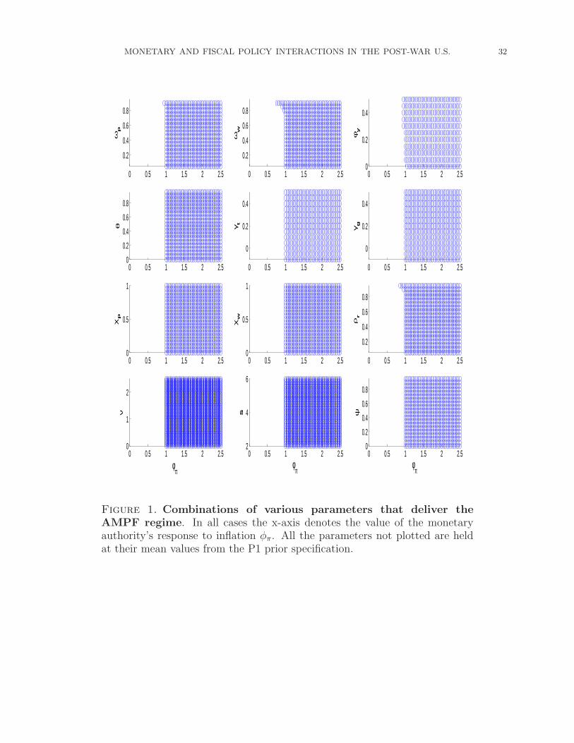
MONETARY AND FISCAL POLICY INTERACTIONS IN THE POST-WAR U.S. 32
0 0.5 1 1.5 2 2.5
0.2
0.4
0.6
0.8ω
p
0 0.5 1 1.5 2 2.5
0.2
0.4
0.6
0.8
ωw
0 0.5 1 1.5 2 2.50
0.2
0.4
φy
0 0.5 1 1.5 2 2.50
0.2
0.4
0.6
0.8
θ
0 0.5 1 1.5 2 2.5
0
0.2
0.4
γt
0 0.5 1 1.5 2 2.5
0
0.2
0.4
γg
0 0.5 1 1.5 2 2.50
0.5
1
χp
0 0.5 1 1.5 2 2.50
0.5
1
χw
0 0.5 1 1.5 2 2.5
0.2
0.4
0.6
0.8
ρr
0 0.5 1 1.5 2 2.50
1
2
φπ
ν
0 0.5 1 1.5 2 2.52
4
6
φπ
s
0 0.5 1 1.5 2 2.50
0.2
0.4
0.6
0.8
φπ
ψ
Figure 1. Combinations of various parameters that deliver theAMPF regime. In all cases the x-axis denotes the value of the monetaryauthority’s response to inflation φπ. All the parameters not plotted are heldat their mean values from the P1 prior specification.
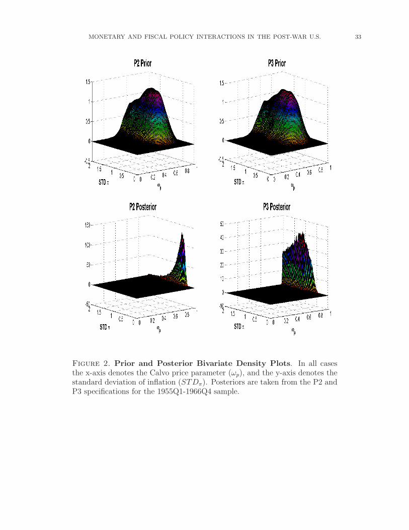
MONETARY AND FISCAL POLICY INTERACTIONS IN THE POST-WAR U.S. 33
Figure 2. Prior and Posterior Bivariate Density Plots. In all casesthe x-axis denotes the Calvo price parameter (ωp), and the y-axis denotes thestandard deviation of inflation (STDπ). Posteriors are taken from the P2 andP3 specifications for the 1955Q1-1966Q4 sample.

MONETARY AND FISCAL POLICY INTERACTIONS IN THE POST-WAR U.S. 34
Figure 3. Prior and Posterior Bivariate Density Plots. In all cases thex-axis denotes the value of the monetary authority’s response to output (φy),and the y-axis denotes the standard deviation of labor (STDL). Posteriorsare taken from the P2 and P3 specifications for the 1955Q1-1966Q4 sample.

MONETARY AND FISCAL POLICY INTERACTIONS IN THE POST-WAR U.S. 35
0 2 4 6 8 10
−4
−2
01955−1966
outp
ut
0 2 4 6 8 10
−4
−2
01967−1979
0 2 4 6 8 10
−4
−2
01984−2007
0 2 4 6 8 10
−0.4
−0.2
0
infla
tion
0 2 4 6 8 10
−0.4
−0.2
0
0 2 4 6 8 10
−0.4
−0.2
0
0 2 4 6 8 10
0
0.5
1
fed
fund
s ra
te
0 2 4 6 8 10
0
0.5
1
years after shock0 2 4 6 8 10
0
0.5
1
Figure 4. The effects of monetary policy across samples: all samplesunder P1. Y-axis is in percentage deviation to the steady state. Solid lines:responses under the mean estimates of the parameters; dotted-dashed lines:90% confidence bands.

MONETARY AND FISCAL POLICY INTERACTIONS IN THE POST-WAR U.S. 36
0 2 4 6 8 10−4
−2
0
1955−1966
outp
ut
0 2 4 6 8 10−4
−2
0
1967−1979
0 2 4 6 8 10−4
−2
0
1984−2007
0 2 4 6 8 10−0.2
−0.1
0
infla
tion
0 2 4 6 8 10−0.2
−0.1
0
0 2 4 6 8 10−0.2
−0.1
0
0 2 4 6 8 10
0
0.5
1
fed
fund
s ra
te
0 2 4 6 8 10
0
0.5
1
years after shock0 2 4 6 8 10
0
0.5
1
Figure 5. The effects of monetary policy across samples: 1955Q1-1966Q4 and 1967Q1-1979Q2 are under P2, and 1984Q1-2007Q4 isunder P1. Y-axis is in percentage deviation to the steady state. Solid lines:responses under the mean estimates of the parameters; dotted-dashed lines:90% confidence bands.
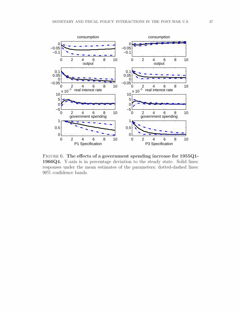
MONETARY AND FISCAL POLICY INTERACTIONS IN THE POST-WAR U.S. 37
0 2 4 6 8 10
−0.1−0.05
0
consumption
0 2 4 6 8 10−0.05
00.05
0.1
output
0 2 4 6 8 10−5
05
10x 10
−3 real interest rate
0 2 4 6 8 100
0.5
1government spending
P1 Specification
0 2 4 6 8 10
−0.1−0.05
0
consumption
0 2 4 6 8 10−0.05
00.05
0.1
output
0 2 4 6 8 10−5
05
10x 10
−3 real interest rate
0 2 4 6 8 100
0.5
1government spending
P3 Specification
Figure 6. The effects of a government spending increase for 1955Q1-1966Q4. Y-axis is in percentage deviation to the steady state. Solid lines:responses under the mean estimates of the parameters; dotted-dashed lines:90% confidence bands.

MONETARY AND FISCAL POLICY INTERACTIONS IN THE POST-WAR U.S. 38
0 2 4 6 8 10−0.1
00.10.2
consumption
0 2 4 6 8 10
0
0.1
0.2output
0 2 4 6 8 10−0.03−0.02−0.01
00.01
real interest rate
0 2 4 6 8 100
0.5
1government spending
P1 Specification
0 2 4 6 8 10−0.1
00.10.2
consumption
0 2 4 6 8 10
0
0.1
0.2output
0 2 4 6 8 10−0.03−0.02−0.01
00.01
real interest rate
0 2 4 6 8 100
0.5
1government spending
P3 Specification
Figure 7. The effects of a government spending increase for 1967Q1-1979Q2. Y-axis is in percentage deviation to the steady state. Solid lines:responses under the mean estimates of the parameters; dotted-dashed lines:90% confidence bands.
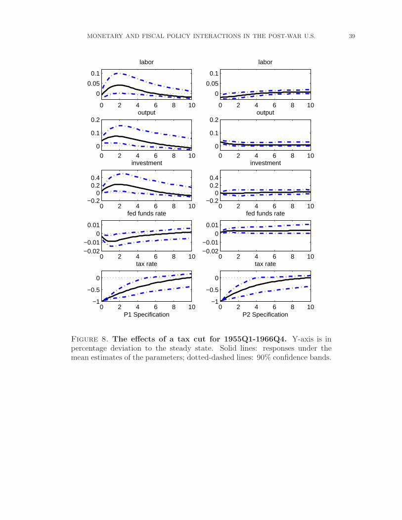
MONETARY AND FISCAL POLICY INTERACTIONS IN THE POST-WAR U.S. 39
0 2 4 6 8 10
0
0.05
0.1
labor
0 2 4 6 8 10
0
0.1
0.2output
0 2 4 6 8 10−0.2
00.20.4
investment
0 2 4 6 8 10−0.02−0.01
00.01
fed funds rate
0 2 4 6 8 10−1
−0.5
0
tax rate
P1 Specification
0 2 4 6 8 10
0
0.05
0.1
labor
0 2 4 6 8 10
0
0.1
0.2output
0 2 4 6 8 10−0.2
00.20.4
investment
0 2 4 6 8 10−0.02−0.01
00.01
fed funds rate
0 2 4 6 8 10−1
−0.5
0
tax rate
P2 Specification
Figure 8. The effects of a tax cut for 1955Q1-1966Q4. Y-axis is inpercentage deviation to the steady state. Solid lines: responses under themean estimates of the parameters; dotted-dashed lines: 90% confidence bands.

MONETARY AND FISCAL POLICY INTERACTIONS IN THE POST-WAR U.S. 40
0 2 4 6 8 10
0
0.05
0.1labor
0 2 4 6 8 10−0.05
00.05
0.1
output
0 2 4 6 8 10−0.2
00.20.4
investment
0 2 4 6 8 10−0.02−0.01
00.01
fed funds rate
0 2 4 6 8 10−1
−0.5
0
tax rate
P1 Specification
0 2 4 6 8 10
0
0.05
0.1labor
0 2 4 6 8 10
00.05
0.1
output
0 2 4 6 8 10−0.2
00.20.4
investment
0 2 4 6 8 10−0.02−0.01
00.01
fed funds rate
0 2 4 6 8 10−1
−0.5
0
tax rate
P2 Specification
Figure 9. The effects of a tax cut for 1967Q1-1979Q2. Y-axis is inpercentage deviation to the steady state. Solid lines: responses under themean estimates of the parameters; dotted-dashed lines: 90% confidence bands.