JOURNAL OF MATHEMATICAL ANALYSIS AND APPLICATIONS 65, 306-320 (1978)

Moment Equation Methods for Nonlinear Stochastic Systems

D. C. C. BOVER

Computer Centre, Australian National University, Canberra, Australia

Submitted by T. T. Soong

One method of approaching models represented by systems of stochastic ordinary differential equations is to consider the moment equations. This approach can be far more efficient than a Monte Carlo simulation or a finite- difference solution of the associated Fokker-Plank equation. However, a non- linear system generates an infinite hierarchy of moment equations, which requires the adoption of some hierarchy truncation technique to facilitate solution. This paper considers a method of hierarchy truncation, based on the quasi- moments of the state-variables.

1. INTRODUCTION

A large class of physical, social, and economic phenomena can be modeled by systems of coupled ordinary differential equations ([I]-[9]). Stochastic models of this type are written in the general form

dx dt = f(x, t) + qx, t) x(t). (1)

Here x(t) is a n x 1 vector of state-variables, f(x, t) is an n x 1 vector repre- senting the deterministic influences in the model, and X(t) is a m x 1 vector of independent random processes which influence the model through the n x m matrixF(x, t). Since the elements ofF(x, t) can be functions of the state variables as well as of time, this class of models includes equations with random coefficients as well as random inhomogeneous terms. The mean parts of the random pro- cesses may be included in f(x, t), thus ensuring that the elements of X(t) all have zero mean.

If we approximate the random processes X(t) by the mathematical idealization of Gaussian white noise processes, the model may be written in the Ito form

dx(t) = f(x, t) dt + F(x, t) dw(t),

306 (2)

OO22-247X/78/0652-0306$02.00/0 Copyright Q 1978 by Academic Press, Inc. All rights of reproduction in any form reserved.

MOMENT EQUATION METHODS 307

where w(t) is a m x 1 vector of independent Gaussian-distributed Wiener processes, each with the properties:

and (q(t)) = (dw,(t)) = 0

((dz~~(t))~) = oi2 dt,

for some real constants cri , for i = 1, 2 ,..., m. Here and throughout this discus- sion, the angle-brackets operation (4(x, t)) on a function 4(x, t) is the expecta- tion, defined by

(4(x, t)) = j-- ... s= 4(x, t) P(x; t) dx, dx2 ... dx, , -m -02 (4)

where P(x; t) is the probability density distribution of the state-variables x. With the exception of a few simple cases, the statistical properties of stochastic

models can be calculated only by numerical techniques, such as a Monte Carlo simulation wherein the moments and distribution are built up over a large number of trials, or a finite-difference solution of the associated Fokker-Plank equation, which leads directly to an approximation for the probability density distribution. The moments of the state-variables can then be calculated by a numerical quadrature procedure. However, even for quite simple models, both of these methods can require considerable computational effort to achieve results of satisfactory accuracy.

An alternative approach is to consider the differential equations for the moments of the state-variables. This method requires much less computation since it involves only the solution of a system of coupled deterministic ordinary differential equations. Also, it leads directly to solutions for the moments of the state-variables, such as their means and variances which are the basic properties that we seek from the model and are the quantities that are directly measurable from physical experiment. The disadvantage of the moment equations is that, except for completely linear models or special cases of nonlinear models, the differential equations for moments of a given order will contain terms involving higher-order moments. We are then faced with an infinite hierarchy of coupled equations which must be approximated by a finite set of equations to facilitate solution.

Bellman and Wilcox [6], in considering the moment equations for a stochastic nonlinear oscillator, tried several methods of hierarchy truncation, the most satisfactory of which was central-cumulant truncation (that is, through obtaining expressions for high-order moments in terms of lower-order moments by assum- ing the high-order central cumulants to be zero). However, no attempt has been made to justify the assumptions basic to cumulant truncation or to explain why that method should give satisfactory results.

This paper presents another method of hierarchy truncation, based on the quasi-moments, which are the coefficients in a multidimensional Hermite

308 D. C. C. BOVER

polynomial expansion of the probability density distribution. The relationship between this method and cumulant truncation is noted and the problem of the stochastic cubic oscillator is used to demonstrate and test the technique.

2. THE MOMENT EQUATIONS

A mixed Kth-order moment of the state-variables may be written as (4(x)), where C(x) = n:=, xfi for nonnegative integers Ki (i = 1, 2,..., n), such that

The differential equation for (4(x)) may be derived either by multiplying both sides of the associated Fokker-Plank equation by d(x) and integrating over the state-space, as suggested in [lo], or directly from the Ito formula for the stochastic differential of 4(x) [l I],

where f, F, and w are as defined in Eqs. (1) and (2) and D is the m x m diagonal matrix with diagonal elements equal to the uz, defined in (3).

Taking the expectation of both sides of (5) gives the general form of the moment equations

(6)

Note that, because of (3) the last term of (5) makes no contribution. In particular, the first-order moment equations are clearly

&x)/dt = <f(x, t)>, (7)

which corresponds to the deterministic model. For higher-order moments it is convenient to consider the central moment equations, defined through the change of variables

y = x - {x). (8)

The model may be written in terms of the central moment variables as

dy = NY + (x>, t) - <f(y + (x>, t)>l dt + F(Y + <x>, t) d-W. (9)

MOMENT EQUATION METHODS 309

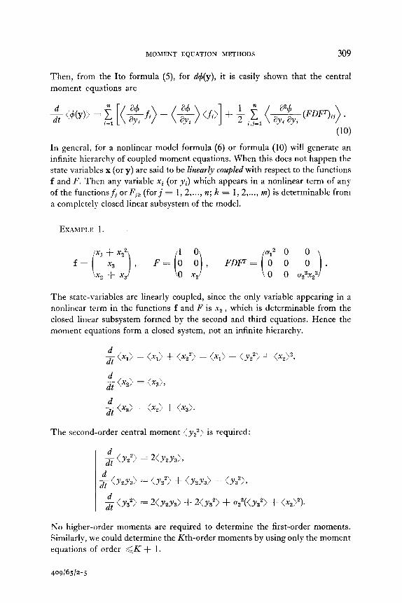
Then, from the Ito formula (5), for d+(y), it is easily shown that the central moment equations are

In general, for a nonlinear model formula (6) or formula (10) will generate an infinite hierarchy of coupled moment equations. When this does not happen the state variables x (or y) are said to be linearly coupEed with respect to the functions f and F. Then any variable xi (or yi) which appears in a nonlinear term of any of the functionsfj or Fjk (forj = 1,2 ,..., n; k = I,2 ,..., m) is determinable from a completely closed linear subsystem of the model.

EXrlMPLE 1.

The state-variables are linearly coupled, since the only variable appearing in a nonlinear term in the functions f and F is x2 , which is determinable from the closed linear subsystem formed by the second and third equations. Hence the moment equations form a closed system, not an infinite hierarchy.

$ (3) = (x1) + (xzZ) = (Xl) + <Y22i + <x2b2,

$ <x2) = xx,>,

$<e = (x2) + (x3).

The second-order central moment (yz2) is required:

$ <Y22> = XY,Y,\>

& (Y2Y3) q = <Y29 + (Y2Y3) + <Y3%

g (Y38) = 2(Y,Y,) + 2(Y32> + %2(<Y22) + <x2)2)-

No higher-order moments are required to determine the first-order moments. Similarly, we could determine the &Ah-order moments by using only the moment equations of order <K + 1.

409/65/2-S

310 D. C. C. BOVER

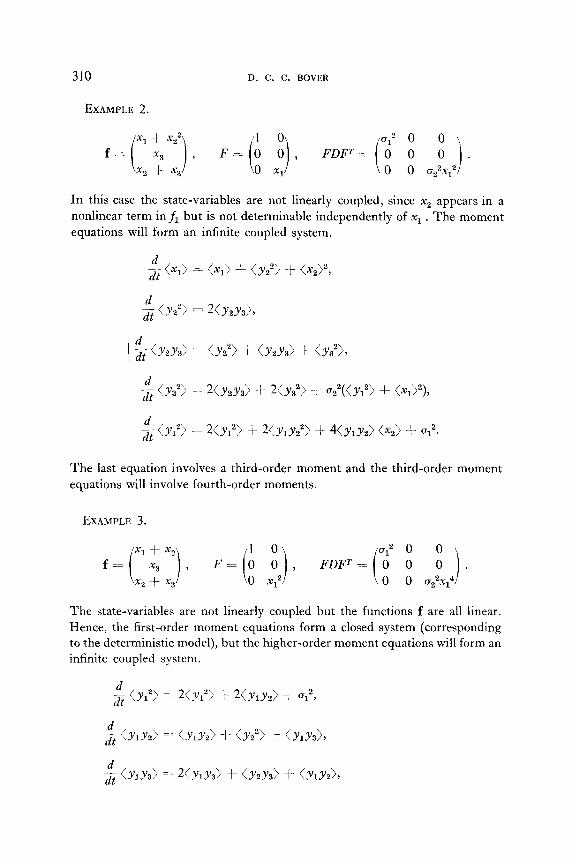
EXAMPLE 2.

In this case the state-variables are not linearly coupled, since x2 appears in a nonlinear term infi but is not determinable independently of xi . The moment equations will form an infinite coupled system.

1 (x1) == (Xl> + <Yz”) + <%?>2,

g <Y29 = XY2YA

g (Y2Ys) = CY2’) + (Y2Y3) + (Ya2),

g <Ys2) =y XY,Y,) + 2<Y,2) + U2”((Yl”> + W2),

g (Yl”> = 2<Yi2) + 2<Y,Y22) + 4(Y,Y2) (x2) + U12.

The last equation involves a third-order moment and the third-order moment equations will involve fourth-order moments.

EXAMPLE 3.

The state-variables are not linearly coupled but the functions f are all linear. Hence, the first-order moment equations form a closed system (corresponding to the deterministic model), but the higher-order moment equations will form an infinite coupled system.

$ (Y12> = KY12) + 2<Y,Y*) + %2,

g <YIY2) = <YIY2> + <Y29 + <YlY3),

g <YlYd = KY,Y,> + (Y2Y3) + <YiY2),

MOMENT EQUATION METHODS 311

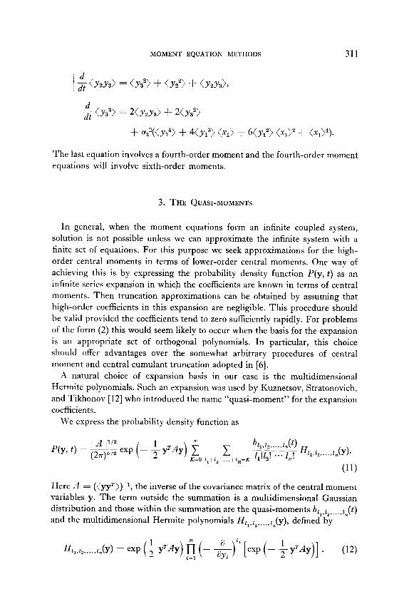
g (Y2Y3) = xY32> + <Y22) + (Y2Ya>,

$ <Y32) = KY,Y,) + XY22)

+ ~2~(<~1~) + 4<y13> (~1) + WY,~) W2 + (~1)~)~

The last equation involves a fourth-order moment and the fourth-order moment equations will involve sixth-order moments.

3. THE QUASI-MOMENTS

In general, when the moment equations form an infinite coupled system, solution is not possible unless we can approximate the infinite system with a finite set of equations. For this purpose we seek approximations for the high- order central moments in terms of lower-order central moments. One way of achieving this is by expressing the probability density function P(y, t) as an infinite series expansion in which the coefficients are known in terms of central moments. Then truncation approximations can be obtained by assuming that high-order coefficients in this expansion are negligible. This procedure should be valid provided the coefficients tend to zero sufficiently rapidly. For problems of the form (2) this would seem likely to occur when the basis for the expansion is an appropriate set of orthogonal polynomials. In particular, this choice should offer advantages over the somewhat arbitrary procedures of central moment and central cumulant truncation adopted in [6].

A natural choice of expansion basis in our case is the multidimensional Hermite polynomials. Such an expansion was used by Kuznetsov, Stratonovich, and Tikhonov [12] who introduced the name “quasi-moment” for the expansion coefficients.

We express the probability density function as

Here il = ((yy’)))‘, the inverse of the covariance matrix of the central moment variables y. The term outside the summation is a multidimensional Gaussian distribution and those within the summation are the quasi-moments !Q~, Jt) and the multidimensional Hermite polynomials Hrl, r,,., ., m(y), defined by

f41.b...,&4 = exp (+ Y~AY) fi (- &,” [exp (- +yrAy)] . (12)

312 D. C. C. BOVER

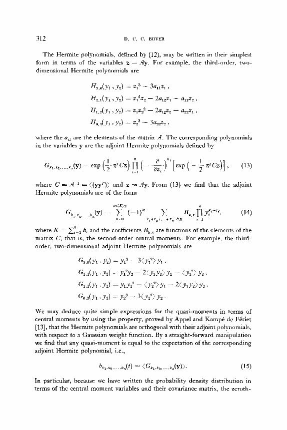
The Hermite polynomials, defined by (12), may be written in their simplest form in terms of the variables z = Ay. For example, the third-order, two- dimensional Hermite polynomials are

ff3,“(Yl 1 YJ = 213 - 3%,% ,

ff2AYl > Y2) = X12Z2 - 2a,,z, - UllZ2 ,

%2(Yl 7 Y2) = %x22 - 2%% - Q22% ,

Jf”,,(Yl ? YJ = z23 - 3%% ,

where the aLj are the elements of the matrix A. The corresponding polynomials in the variables y are the adjoint Hermite polynomials defined by

where C = A-l = ((yyr)) and z = Ay. From (13) we find that the adjoint Hermite polynomials are of the form

RQKIB

Gkl.k,....,k, (Y) = c (-OR rl+T +F+r =2R BlLr ii YC (14) R=O 2" n i=l

where K = xr=l ki and the coefficients B,,, are functions of the elements of the matrix C, that is, the second-order central moments. For example, the third- order, two-dimensional adjoint Hermite polynomials are

G3,0(~1 ,~2) =y13 - 3(~1’)~1 7

GJ(Y, > ~2) = YI'Y~ - XY,Y~)Y~ - <y12)yz 7

G,,(Y~ >yz) =Y~Y: - <YZ")Y~ - KY,Y,)Y,,

G,,,(Y, 3 YZ) =yz3 - 3<~,2)yz -

We may deduce quite simple expressions for the quasi-moments in terms of central moments by using the property, proved by Appel and KampC de FCriet [13], that the Hermite polynomials are orthogonal with their adjoint polynomials, with respect to a Gaussian weight function. By a straight-forward manipulation we find that any quasi-moment is equal to the expectation of the corresponding adjoint Hermite polynomial, i.e.,

bpks.. .I&) = (G,.t,, . . .k,(~))- (‘5)

In particular, because we have written the probability density distribution in terms of the central moment variables and their covariance matrix, the zeroth-

MOMENT EQUATION METHODS 313

order quasi-moment is equal to 1 and the first- and second-order quasi-moments are all zero. From (14) the expectation of the adjoint polynomial is

R4Kl2

<G. Al,n2,...,kp)) = c FUR R=O Tl, T,+c,,,;-2R B&r @ye . (16)

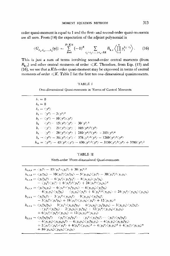
This is just a sum of terms involving second-order central moments (from Bk,r) and other central moments of order <K. Therefore, from Eqs. (15) and (16) we see that a Kth-order quasi-moment may be expressed in terms of central moments of order <K. Table I list the first ten one-dimensional quasimoments.

TABLE I

One-dimensional Quasi-moments in Terms of Central Moments

h, = 0

b, = 0

b., = <Y">

b, == :y4) - 3(y”)=

bz = <Y"> - ~O<Y~><Y">

b, = iy6> - 15:y2>(y”) -t- 30(~9~

b, = <y’> - 21<y2>(y5> + 105<yz,“<y3>

b, = <ye> - 28<y2>Cya> i 2lO(y”>‘(y*> - 315(y”>*

b,, = iy9) - 36(y2><y’> + 378(y2)Yys) - 1260(y*)3iy3j

b,, = /y’“> - 45(y”>(ys> + 630<y2)2(y6> - 3150(y2)3(yr) + 3780<y2j5

TABLE II

Sixth-order Three-dimensional Quasi-moments

b 6.0,0 = <Yl”> - 15<Y,?>(Y14> + 3O<Y,2>3

km =T <Y15Y1> - lWY12><Y13Y2> - 5<Y,Y,><Y,‘> + 3O<Y,WY,Y,> b as3.0 = <YI.‘Y~‘> - 6<~1’><~142~i ~ 8<~1uz><r1~yz>

- <ys’>(~1~j + ~<Y,~>~<Y,~> + 24(~,~)<y,y,>” b 4,1,1 = <Y,~Y~YJ ~ 6<3’1”>(~1~~2~3> - 4<~1vz><y1~ya>

- ~<YIYR><Y~~Y~> - (Y,Y,><YI*> + ~(Y,~>~<Y,Y,> -t ~~<Y,~)(Y,YXY,Y~> b 3,8.0 = CY13Y23> - 3<Y,V(Y,Y,3j - 9<Y1Yz><Y1zY2zj

- ~!Y,‘)(Y,~Y~> + 18<~1~><~1vzj<~z*> + 12:y,y,j3 b 3.2.1 = (YI~YZ’Y.~ - ~<Y~“><YIY~~Y~> - 6<~1yz><y1*yy2~3> - 3<~1~3><~1~~~‘>

- (Y22><Ylh> - 2<YzY3j<Y13Yzj + lXY,2>(Y,Y,><Y,Y,> -t 6<~,~><~2~><~1~3> + 12<~1~,>‘<~1~,>

b 2.2.2 = ~Y12Y**Ys"> - <Yl"><Y2*Y32> - <Yz"><Y12Y82> - <Y32)<Y12Y22>

-- 4<Y,Yz><Y1Y,Y:,2j - 4<YzY~><Y12YzY3> - 4<Y1Y3>(YIY22Y3> + 2<Y12><Yzz><Y32> -t 4<Y,2><Y,Y,>z + 4<Y,2>(Y,Y,>S + 4<Y,S?(Y*Y,>= -;- ~~(Y,Y,>(Y,Y,><Y,Y:~)

314 D. C. C. BOVER

It is not difficult to generalize the one-dimensional moments to several dimen- sions (e.g., see Table II for a list of the sixth-order three-dimensional quasi- moments).

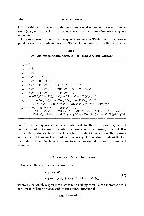
It is interesting to compare the quasi-moments in Table I with the corres- ponding central cumulants, listed in Table III. We see that the third-, fourth-,

TABLE III

One-dimensional Central Cumulants in Terms of Central Moments

K1 = 0

K2 = <Y">

KS rz <Y3> Kq = <y”> - 3(y2>?

KF, = <Y”> -- 10(Y2><Y3> Kg = (y”j - 15:yq<y4> + 3o<y=>3 - lO(y3)”

Ki = fy ‘> - 21(Y%Y5) + 210(Yz>z<Y3> ~ 35<Y%Y”)

~8 -2 <Y*> ~ 28(yz>(y6) + ~~O(Y~>~<Y~) - 630(y2>* - 56;y3><y5> - 35<~~)~ + 560<y2)<y3)2

K~ -= <: yY‘: - 36( y2)( y’) -I- 756< Y~>~( y5> - 7560<~=)~< y3> ~ 84<y%y”> ~ 126(y”><y5> + 252O(y’><y”><y*? + 560<~~)~

sr10 = /y”‘) -. 45(y2)(ys) + 1260(y2)2(y6) - 18900(y2)3(y4) + 22680(y2)5 - 12O<y”)<y’> - 210(y4)(y”) - 126<~~>~ + 5040<y2>(y3)<y5) + 315O(~~)<y’)~ + 4200<y3>2<y4) - 37800(y2>2<y3)~

and fifth-order quasi-moments are identical to the corresponding central cumulants but that above fifth-order, the two become increasingly different. It is this similarity that explains why the central cumulant truncation method proves satisfactory, at least for lower orders of accuracy. The relative merits of the two methods of hierarchy truncation are best demonstrated through a numerical example.

4. STOCHASTIC CUBIC OSCILLATOR

Consider the stochastic cubic oscillator

dx, = x2 dt,

dx, = -((Ax, + Bx13 + x1) dt + dw(t), (17)

where dw(t), which respresents a stochastic driving force, is the increment of a zero-mean Wiener process with mean-square differential

([dw(t)]2) = u2 dt,

MOMENT EQUATION METHODS 315

for a real constant cr. Also A and B are constants representing the damping and cubic spring properties of the oscillator. The model (17) may be written in the standard form (2) if we define

FZZ D = (u2),

then

The first-order moment equations for this model are

y = (x2), (18)

4x2) -- = -4X2) - wcY13) + 3(Y12) <Xl) + (x1)3)- (x1). dt (19)

For higher-order moments, the central moment equations may be generated from formula (10). For example, the second-order central moment equations are

4 x2) - = 2(Y,Y,), dt

d(y& -- = (Y2”> - 4Y,Y2> - B(<Y14) + 3<%)<Y13) + 3<G2(y12))-(y1z> dt

4 ya2) ~ = --24Y,2) - 2B((Y,"Yz) -t 3(x,) <.?Jl”Y2> + 3<~1>2<y1y2)) dt

- XY,Y,) + fJ2.

An important feature of these and all higher-order moment equations is that the Kth-order equations involve moments of order K + 1 and K + 2. So a Kth-order hierarchy truncation method will require approximations for the (K + I)th- and (K + 2)th-order moments.

The results from the moment equations can be tested both in the time- dependent solution against numerical results from a Monte Carlo simulation and in the stationary solution against some analytical properties of the Fokker-Plank equation. For a Monte Carlo simulation, the stochastic model (2) is written as

dx(t) = f(x, t) dt + F(x, t) r(t),

316 D. C. C. BOVER

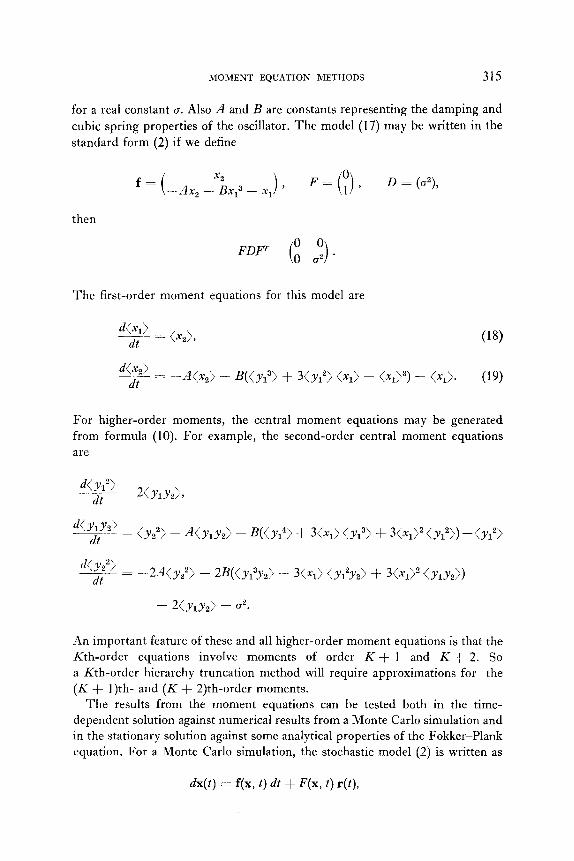
where r(t) = dw(t). The elements of r(t) are Gaussian random numbers with zero mean and with variances (r(t)2) = u2 dt. The time-dependent results for the cubic oscillator (17) from Monte Carlo simulation and both central cumulant and quasi-moment truncation are shown in Fig. 1.

2

FIG. 1. Time-dependent solution for stochastic cubic oscillator, for the case where A = 1.0, B = 0.2, 9 = 5.0. p, moment equation solution (using quasi-moment or cumulant truncation); l , Monte Carlo simulation.

For the stationary solution, we may use the analytical properties suggested by Morton and Corrsin [14], that the stationary mean-square displacement and the kurtosis of the displacement have the functional forms

(20)

(21)

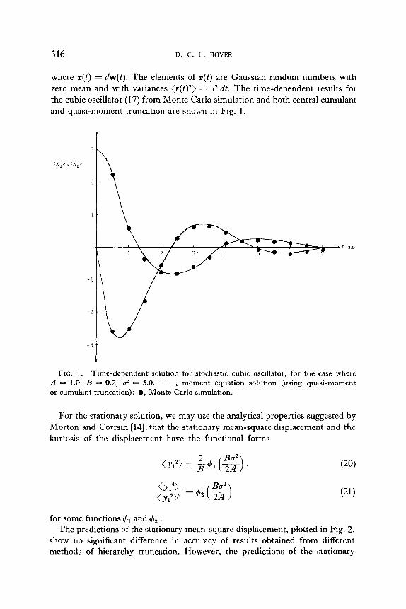
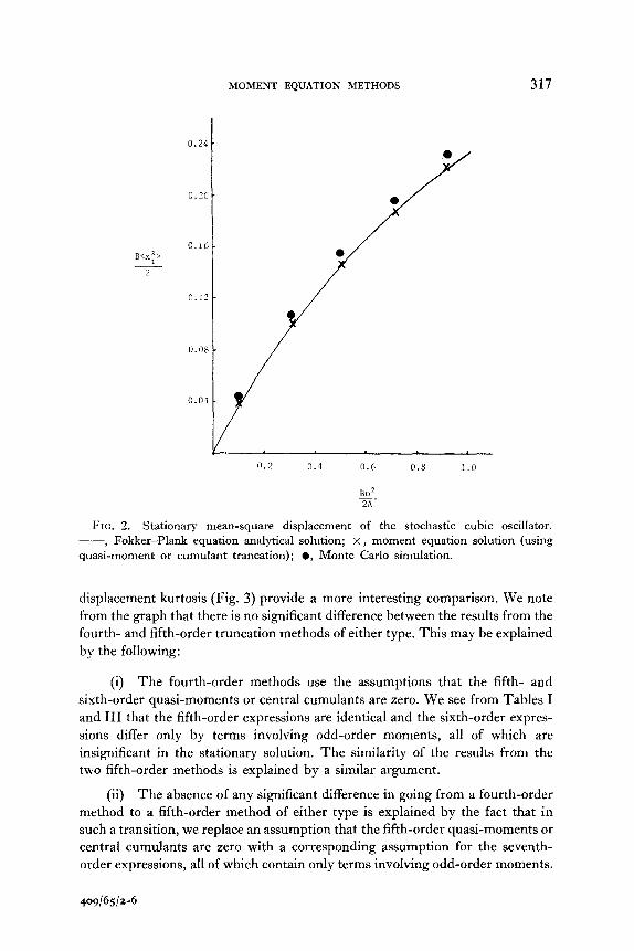
for some functions Q1 and 4z . The predictions of the stationary mean-square displacement, plotted in Fig. 2,

show no significant difference in accuracy of results obtained from different methods of hierarchy truncation. However, the predictions of the stationary

MOMENT EQUATION METHODS 317

0.24

0.20

0.16 B<x'> 1

2

0.11

0.08

0.2 0.4 0.6 0.8 1.0

FIG. 2. Stationary mean-square displacement of the stochastic cubic oscillator. --, Fokker-Plank equation analytical solution; x , moment equation solution (using quasi-moment or cumulant trancation); l , Monte Carlo simulation.

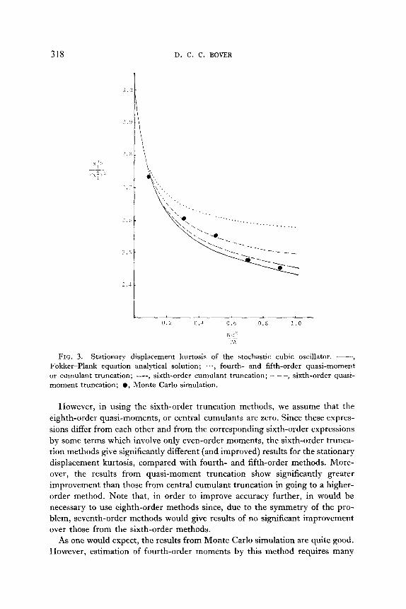
displacement kurtosis (Fig. 3) provide a more interesting comparison. We note from the graph that there is no significant difference between the results from the fourth- and fifth-order truncation methods of either type. This may be explained by the following:

(i) The fourth-order methods use the assumptions that the fifth- and sixth-order quasi-moments or central cumulants are zero. We see from Tables I and III that the fifth-order expressions are identical and the sixth-order expres- sions differ only by terms involving odd-order moments, all of which are insignificant in the stationary solution. The similarity of the results from the two fifth-order methods is explained by a similar argument.

(ii) The absence of any significant difference in going from a fourth-order method to a fifth-order method of either type is explained by the fact that in such a transition, we replace an assumption that the fifth-order quasi-moments or central cumulants are zero with a corresponding assumption for the seventh- order expressions, all of which contain only terms involving odd-order moments.

409/w2-6

318 D. C. C. BOVER

0.1 0 .I 0 (1 0.s 1.0

Ii L.1 2.k

FIG. 3. Stationary displacement kurtosis of the stochastic cubic oscillator. --, Fokker-Plank equation analytical solution; ..., fourth- and fifth-order quasi-moment or cumulant truncation; ----, sixth-order cumulant truncation; - - -, sixth-order quasi- moment truncation; l , Monte Carlo simulation.

However, in using the sixth-order truncation methods, we assume that the eighth-order quasi-moments, or central cumulants are zero. Since these expres- sions differ from each other and from the corresponding sixth-order expressions by some terms which involve only even-order moments, the sixth-order trunca- tion methods give significantly different (and improved) results for the stationary displacement kurtosis, compared with fourth- and fifth-order methods. More- over, the results from quasi-moment truncation show significantly greater improvement than those from central cumulant truncation in going to a higher- order method. Note that, in order to improve accuracy further, in would be necessary to use eighth-order methods since, due to the symmetry of the pro- blem, seventh-order methods would give results of no significant improvement over those from the sixth-order methods.

As one would expect, the results from Monte Carlo simulation are quite good. However, estimation of fourth-order moments by this method requires many

MOMENT EQUATION METHODS 319

more trials than are necessary for good estimates of second-order moments. The moment equation methods offer a significant reduction in computation. Even when the number of nlonte Carlo trials was too low to give reasonable estimates of the fourth-order moments, though high enough for good estimates of the second-order moments, the computer time for solution by moment equa- tion methods was about l/60 of the time taken for Monte Carlo simulation, and about I /I 80 of the time for a finite-difference solution of the Fokkcr-Plank equation. However, only rough estimates were used for the optimal parameters in the iteration method of solution of the Fokker-Plank equation.

The programming effort involved in moment equation methods is naturally greater than that for Monte Carlo simulation. However, the quasi-moments can be fairly easily generated since they are related to the Hermite polynomials, whereas automatic generation of central cumulants would be a rather difficult programming task.

ACKNOWLEDGMENTS

The author wishes to thank Dr. M. R. Osborne and Dr. R. 0. Watts for helpful discussions, and the referee for comments which have assisted in improving the presenta- tion of this paper.

1. S. CHANDRASEKHAR, Stochastic problems in physics and astronomy, Reo. Modern Phys. 15 (1943), 1-89.

2. J. E. MOYAL, Stochastic processes and statistical physics, J. Roy. Statist. Sm. Ser. B 11 (1949), 1.50-210.

3. T. Ii. CAUGHEY, Derivation and application of the Fokker-Plank equation to discrete nonlinear dynamic systems subjected to white random excitation, J. Acoust. Sac. Amer. 35 (1963), 1683-1692.

4. R. L. STRATONOVICH, “Topics in the Theory of Random Noise,” Vol. 2, Gordon & Breach, New York, 1963.

5. S. C. LILT, Solutions of Fokker-Plank equation with applications in nonlinear random vibration, Bell System Tech. J. 48 (1969), 2031-2051.

6. R. BELLMAN AND R. M. WILCOX, Truncation and preservation of moment properties for Fokker-Plank moment equations, J. Math. Anal. Appl. 32 (1970), 532-542.

7. N. G. F. SANCHO, Technique for finding the moment equations of a nonlinear stochastic system, J. Math. Phys. 11 (1970), 771-774.

8. N. S. GOEL, S. C. MAITRA, AND E. W. MONTROLL, On the Volterra and other non- linear models of interacting populations, Rev. Modem Phys. 43 (1971), 231-276.

9. M. LEVISON, R. G. WARD, AND J. W. WEBB, “The Settlement of Polynesia. A Computer Simulation,” A.N.U. Press, Canberra, 1973.

10. S. T. ARIARATNAM AND P. W. U. GRAEFE, Linear systems with stochastic coefficients, Intermt. J. Control 1 (1965), 239-250.

11. I. I. GIHMAN AND A. V. SKOROHOD, “Stochastic Differential Equations,” pp. 263-272, Springer-Verlag, New York, 1972.

320 D. C. C. BOVER

12. P. I. KUZNETSOV, R. L. STRATONOVICH, AND V. I. TIKHONOV, Quasi-moment functions in the theory of random processes, Theou. Probability Appl. 5 (1960), 80-97.

13. P. APPEL AND J. KAMPB DE FCRIET, “Fonctions hypergeometriques et hyperspheriques. Polynomes d’Hermite,” pp. 367-369, Gauthier-Villars, Paris, 1926.

14. J. B. MORTON AND S. CORRSIN, Experimental confirmation of the applicability of the Fokker-Plank equation to a nonlinear oscillator, J. Math. Phys. 10 (1969), 361-368.