Embed Size (px)
Citation preview
Developed by Moly-Cop Grinding SystemsS
ett
ing
Ne
w S
tan
da
rd M
eth
od
olo
gie
s in
Se
ttin
g N
ew
Sta
nd
ard
Me
tho
do
log
ies
in
Gri
nd
ing
Pro
ce
ss
An
aly
sis
Gri
nd
ing
Pro
ce
ss
An
aly
sis

Podremos moler mas Podremos moler mas ToneladasToneladas
Si alimentamos Si alimentamos mas fino...?mas fino...?
Podremos aumentarPodremos aumentarLa potencia del La potencia del
MolinoMolino
Necesitaremos ciclonesNecesitaremos ciclonesMas Grandes....?Mas Grandes....?
Necesitare cambiar de Necesitare cambiar de Bombas..?Bombas..?
Deberiamos añadirDeberiamos añadirMas agua..?Mas agua..? Como Afectara el nuevo Como Afectara el nuevo
Mineral a los molinos..?Mineral a los molinos..?
Necesitaremos umNecesitaremos umMolino mas...?Molino mas...?
Cual sera la configuraciónCual sera la configuraciónIdeal del cicuito.? SAG o sin SAG..?Ideal del cicuito.? SAG o sin SAG..?
En la mente de un ‘estudioso’ Ingeniero de procesos

Se
ttin
g N
ew
Sta
nd
ard
Me
tho
do
log
ies
in
Se
ttin
g N
ew
Sta
nd
ard
Me
tho
do
log
ies
in
Gri
nd
ing
Pro
ce
ss
An
aly
sis
Gri
nd
ing
Pro
ce
ss
An
aly
sis
MolyMoly--Cop ToolsCop ToolsMolyMoly--Cop ToolsCop Tools

Moly-Cop Tools es un conjunto de planillas EXCEL2000
Moly-Cop Tools es un conjunto de planillas EXCEL2000
diseñadas para ayudar al Ingeniero de Procesos a
caracterizar la eficiencia operacional de un determinado
circuito de molienda, en base a metodologías y criterios de
amplia aceptación práctica.
Moly-Cop Tools comprende una amplia gama de simuladores
para la molienda convencional y semiautógena bajo las
configuraciones más usuales; más algunas planillas
complementarias referentes a la Ley de Bond, el „algebra‟ de
las cargas de bolas y otras de utilidad general.
Moly-Cop Tools está disponible, bajo licencia sin cargo, a
través de la organización Moly-Cop.
MolyMoly--Cop ToolsCop Tools
DE QUÉ SE TRATA ?DE QUÉ SE TRATA ?MolyMoly--Cop ToolsCop Tools
DE QUÉ SE TRATA ?DE QUÉ SE TRATA ?
Moly-Cop Tools está diseñado para operar en
Moly-Cop Tools está diseñado para operar en
ambiente EXCEL 2000 y por lo tanto, es fácilmente
accesible para cualquier Ingeniero de Procesos con
conocimientos básicos de planillas de cálculo.
A diferencia de otros desarrollos anteriores, Moly -
Cop Tools tiene compatibilidad con otras
aplicaciones de Office 2000 y equipos periféricos.
Moly-Cop Tools imprime los resultados en formatos
flexibles, fácilmente adaptables a las necesidades
de cada ususario.
MolyMoly--Cop ToolsCop Tools
LA VENTAJALA VENTAJA
MolyMoly--Cop ToolsCop Tools
LA VENTAJALA VENTAJA

Moly-Cop Tools TM : Theoretical Framework
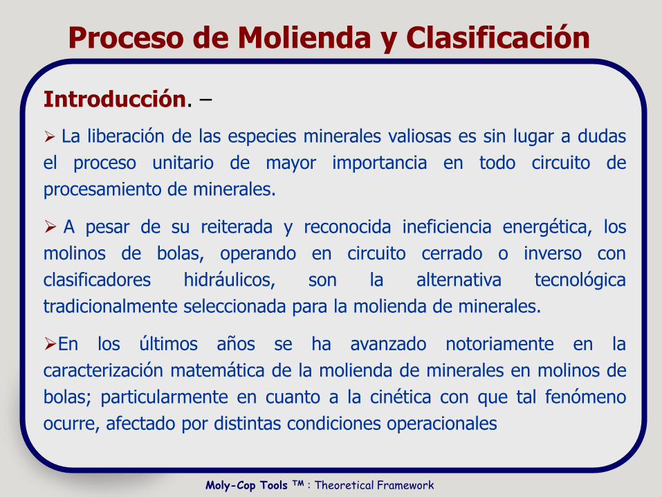
Proceso de Molienda y Clasificación
Introducción. –
La liberación de las especies minerales valiosas es sin lugar a dudas
el proceso unitario de mayor importancia en todo circuito de
procesamiento de minerales.
A pesar de su reiterada y reconocida ineficiencia energética, los
molinos de bolas, operando en circuito cerrado o inverso con
clasificadores hidráulicos, son la alternativa tecnológica
tradicionalmente seleccionada para la molienda de minerales.
En los últimos años se ha avanzado notoriamente en la
caracterización matemática de la molienda de minerales en molinos de
bolas; particularmente en cuanto a la cinética con que tal fenómeno
ocurre, afectado por distintas condiciones operacionales
Moly-Cop Tools TM : Theoretical Framework
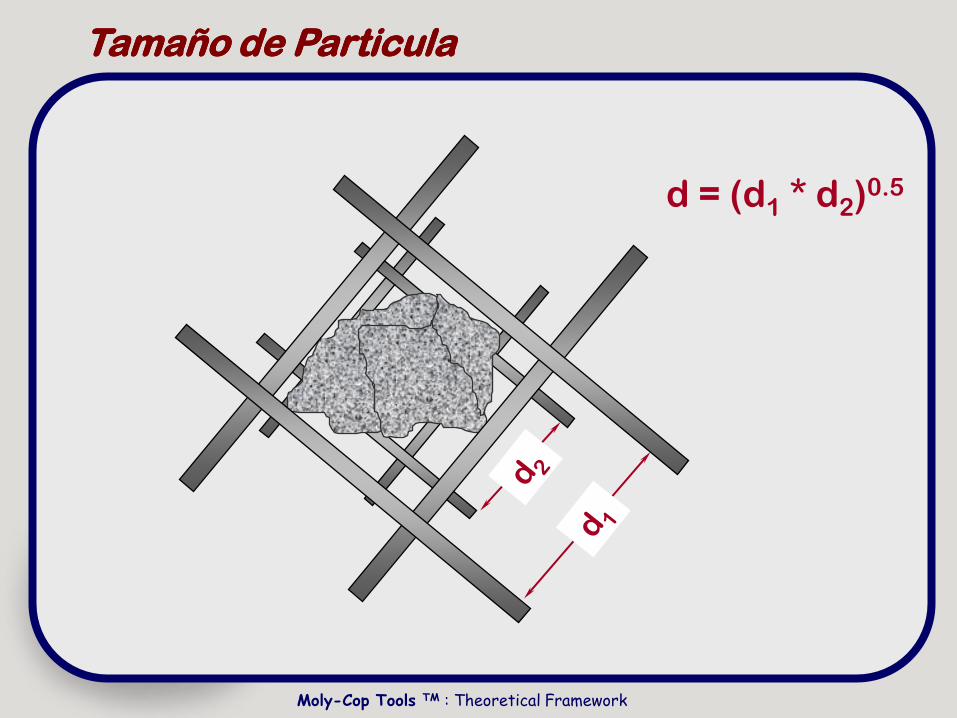
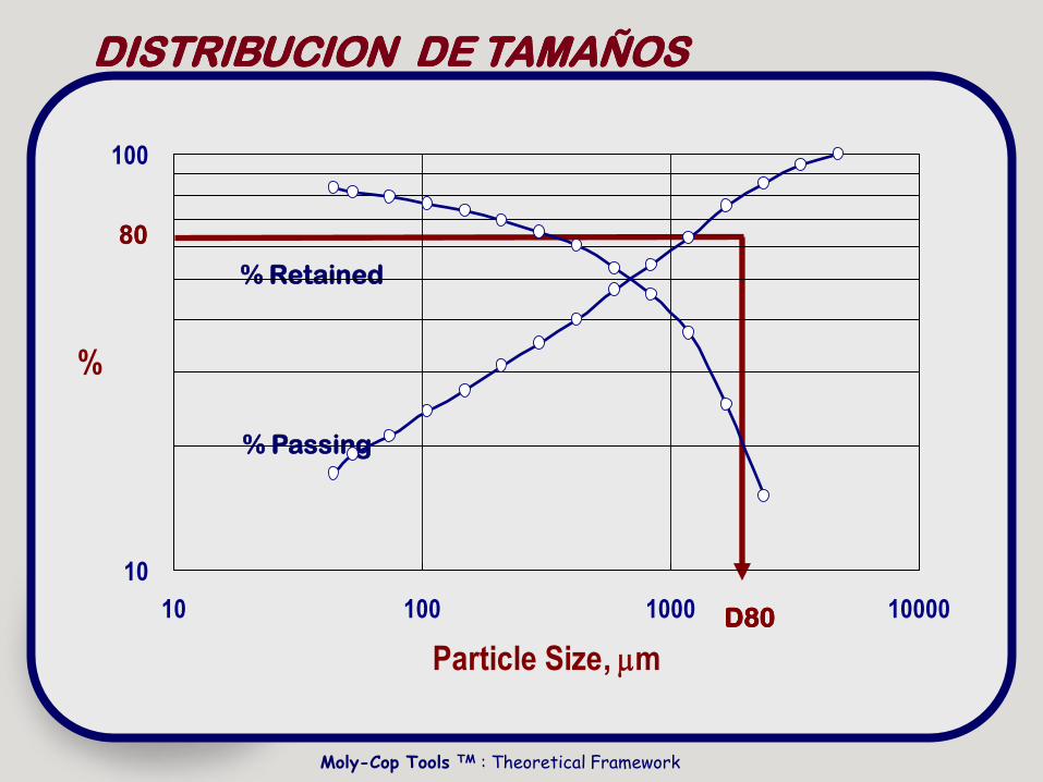
Tamaño de ParticulaTamaño de Particula
d = (d1 * d2)0.5
Moly-Cop Tools TM : Theoretical Framework
DISTRIBUCION DE TAMAÑOSDISTRIBUCION DE TAMAÑOS
% Retained
% Passing
D80D80
8080
10
100
10 100 1000 10000
Particle Size, mm
%
Moly-Cop Tools TM : Theoretical Framework
10
100
10 100 1000 10000
Particle Size, mm
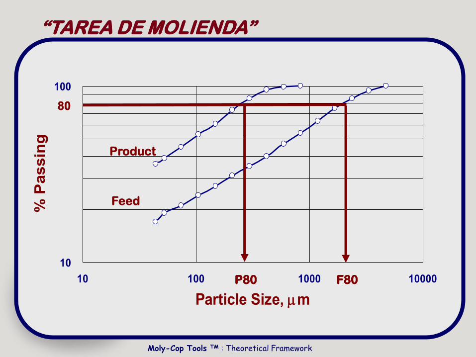
% P
assin
g
P80P80 F80F80
8080
“TAREA DE MOLIENDA”“TAREA DE MOLIENDA”
Product
Feed
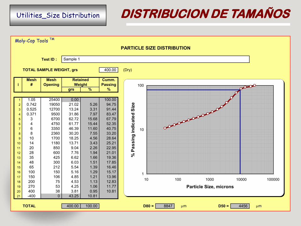
DISTRIBUCION DE TAMAÑOSDISTRIBUCION DE TAMAÑOS
Moly-Cop Tools TM
Test ID :
TOTAL SAMPLE WEIGHT, grs 400.00 (Dry)
Mesh Mesh Cumm.
i # Opening Passing
grs % %
1 1.05 25400 0.00 100.00
2 0.742 19050 21.02 5.26 94.75
3 0.525 12700 13.24 3.31 91.44
4 0.371 9500 31.86 7.97 83.47
5 3 6700 62.72 15.68 67.79
6 4 4750 61.77 15.44 52.35
7 6 3350 46.39 11.60 40.75
8 8 2360 30.20 7.55 33.20
9 10 1700 18.25 4.56 28.64
10 14 1180 13.71 3.43 25.21
11 20 850 9.04 2.26 22.95
12 28 600 7.76 1.94 21.01
13 35 425 6.62 1.66 19.36
14 48 300 6.03 1.51 17.85
15 65 212 5.54 1.39 16.46
16 100 150 5.16 1.29 15.17
17 150 106 4.85 1.21 13.96
18 200 75 4.53 1.13 12.83
19 270 53 4.25 1.06 11.77
20 400 38 3.81 0.95 10.81
21 -400 0 43.25 10.81
TOTAL 400.00 100.00 D80 = 8847 mm D50 = 4456 mm
Retained
Weight
PARTICLE SIZE DISTRIBUTION
Sample 1
1
10
100
10 100 1000 10000 100000
Particle Size, microns
% P
as
sin
g in
dic
ate
d S
ize
Utilities_Size Distribution
Moly-Cop Tools TM : Theoretical Framework
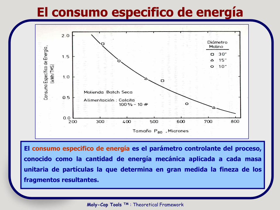
El consumo especifico de energía
El consumo especifico de energía es el parámetro controlante del proceso,
conocido como la cantidad de energía mecánica aplicada a cada masa
unitaria de partículas la que determina en gran medida la fineza de los
fragmentos resultantes.

“Existe una relacion entre el“Existe una relacion entre elConsumo Especifico de EnergiaConsumo Especifico de Energiay el y el Resultante..........Resultante..........
Es decir:Es decir:
“Existe una relacion entre el“Existe una relacion entre elConsumo Especifico de EnergiaConsumo Especifico de Energiay el y el tamaño de productotamaño de productoResultante..........Resultante..........
Es decir:Es decir:
A mas A mas kWh/tonkWh/ton, menor , menor P80P80 !!
Moly-Cop Tools TM : Theoretical Framework
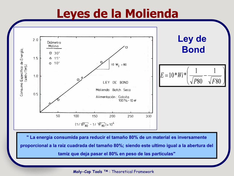
Leyes de la Molienda
" La energía consumida para reducir el tamaño 80% de un material es inversamente
proporcional a la raíz cuadrada del tamaño 80%; siendo este ultimo igual a la abertura del
tamiz que deja pasar el 80% en peso de las partículas"
80
1
80
1**10
FPWiE
Ley de
Bond

Moly-Cop Tools TM : Theoretical Framework
En la expresión anterior el par F80 y P80 se les denomina tarea de molienda; así mismo
permite estimar la energía (Kwhr) requerida para moler cada unidad (ton) de mineral.
Resulta Obvio que un aumento en la potencia (P), debiera traducirse en un aumento de
la capacidad (M)
M
PE
Leyes de la Molienda
Ley de
Bond
Moly-Cop Tools TM : Theoretical Framework
4
5
6
7
8
9
10
11
12
80 100 120 140 160 180 200 220 240 260
Product Size, mm
Sp
ec
ífic
En
erg
y,
kW
h/t
on
Feed Size
4000 mm
2000 mm
1000 mm
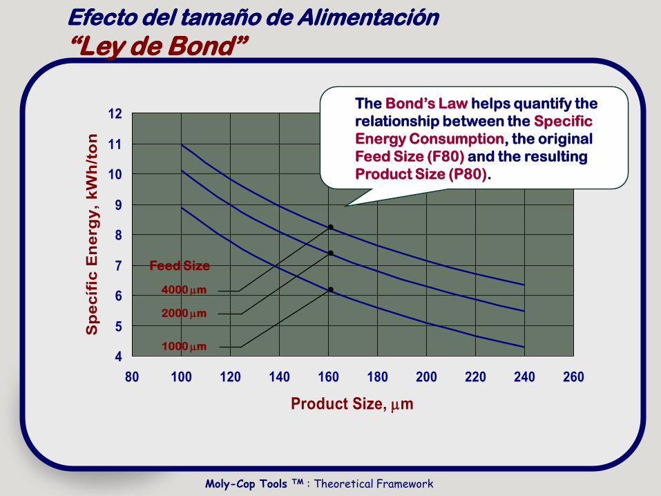
The Bond‟s Law helps quantify the
relationship between the Specific
Energy Consumption, the original
Feed Size (F80) and the resulting
Product Size (P80).
Efecto del tamaño de Alimentación Efecto del tamaño de Alimentación
“Ley de Bond”“Ley de Bond”
Moly-Cop Tools TM : Theoretical Framework
Limitaciones y deficiencias de las teorías clásicas de la conminución
Primero, el procedimiento de Bond utiliza un solo tamiz de
separación para simular la malla de corte, es decir se realiza una
“clasificación ideal”, lo cual es imposible de alcanzar a nivel
industrial.
Segundo, las condiciones de equilibrio alcanzadas en un test de
laboratorio corresponden a estado estacionario alcanzado en un
molino “plug flow” de flujo piston. Es decir en el metodo de Bond
no considera que los molinos no actuan como mezcladores de
pulpa ademas de moler las particulas de mineral. Las
caracteristicas dinámicas de transporte de pulpa en el molino
normalmente se situan entre los casos extremos de mezcla
perfecta y flujo piston.
Moly-Cop Tools TM : Theoretical Framework
Limitaciones y deficiencias de las teorías clásicas de la conminución
Tercero, se supone también en forma implícita que todos los
materiales se fracturan de una manera similar, es decir de acuerdo
a las características típicas de un “material ideal“ dicho material se
caracteriza por tener una distribución RR, con una pendiente igual
a 0.5.
Cuarto, en el método de Bond se utilizan solo 3 parámetros para
calcular el consumo de energía en la molienda, ellos son el WI, F(0
y P80, el concepto de Wi, engloba todo el proceso de fractura, es
por ello que se ha debido incluir una serie de factores de
corrección a fin de tomar en cuenta el efecto de diversas variables
de operación.
Moly-Cop Tools TM : Theoretical Framework
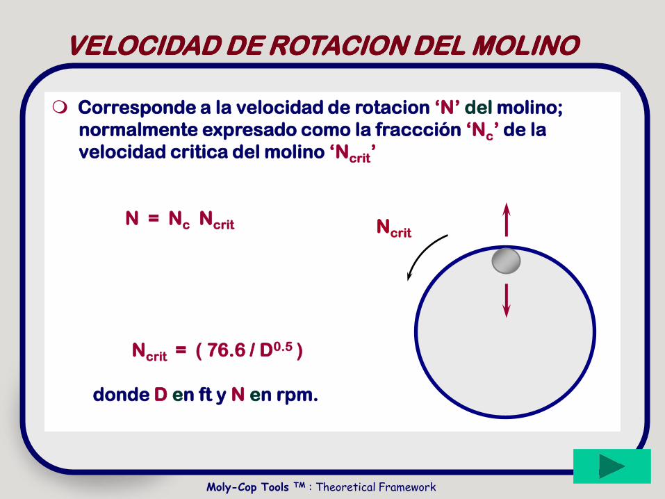
Corresponde a la velocidad de rotacion „N‟ del molino;
normalmente expresado como la fraccción „Nc‟ de la
velocidad critica del molino „Ncrit‟
N = Nc Ncrit
Corresponde a la velocidad de rotacion „N‟ del molino;
normalmente expresado como la fraccción „Nc‟ de la
velocidad critica del molino „Ncrit‟
N = Nc Ncrit Ncrit
VELOCIDAD DE ROTACION DEL MOLINOVELOCIDAD DE ROTACION DEL MOLINO
Ncrit = ( 76.6 / D0.5 )
donde D en ft y N en rpm.
Moly-Cop Tools TM : Theoretical Framework
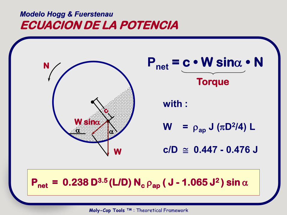
Modelo Hogg & FuerstenauModelo Hogg & Fuerstenau
ECUACION DE LA POTENCIAECUACION DE LA POTENCIA
W sinW sin
WW
NN Pnet = c • W sin • N
Torque
with :
W = rap J (pD2/4) L
c/D 0.447 - 0.476 J
PPnetnet = 0.238 D= 0.238 D3.5 3.5 (L/D) N(L/D) Ncc rrapap ( J ( J -- 1.065 J1.065 J2 2 ) s) siin n
0.0000
0.0100
0.0200
0.0300
0.0400
0.0500
0 5 10 15 20 25 30 35 40 45
Effective Mill Diameter, ft
(kW
h/t
on
)/re
v
.
Conventional SAG
J = 26 %
= 40 °
J = 38 %
= 32 °
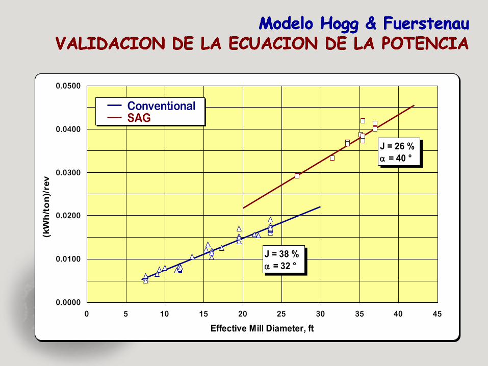
Modelo Hogg & FuerstenauModelo Hogg & FuerstenauVALIDACION DE LA ECUACION DE LA POTENCIAVALIDACION DE LA ECUACION DE LA POTENCIA
Modelo Hogg & FuerstenauModelo Hogg & FuerstenauVALIDACION DE LA ECUACION DE LA POTENCIAVALIDACION DE LA ECUACION DE LA POTENCIA

No basta con tener
Potencia disponible,
también hay que saber
Usarla con Eficiencia !

Moly-Cop Tools TM : Theoretical Framework
AREA ESPECIFICA DE LA CARGA DE BOLASAREA ESPECIFICA DE LA CARGA DE BOLAS
Se ha demostrado que la variable única y controlante del
efecto de la carga de bolas sobre los parámetros cinéticos
es su áreaárea específicaespecífica “a”,“a”, definida como la superficie
expuesta al impacto (m2) por unidad de volumen aparente
de carga (m3)
af
d
v
B
R
8000 1*( )
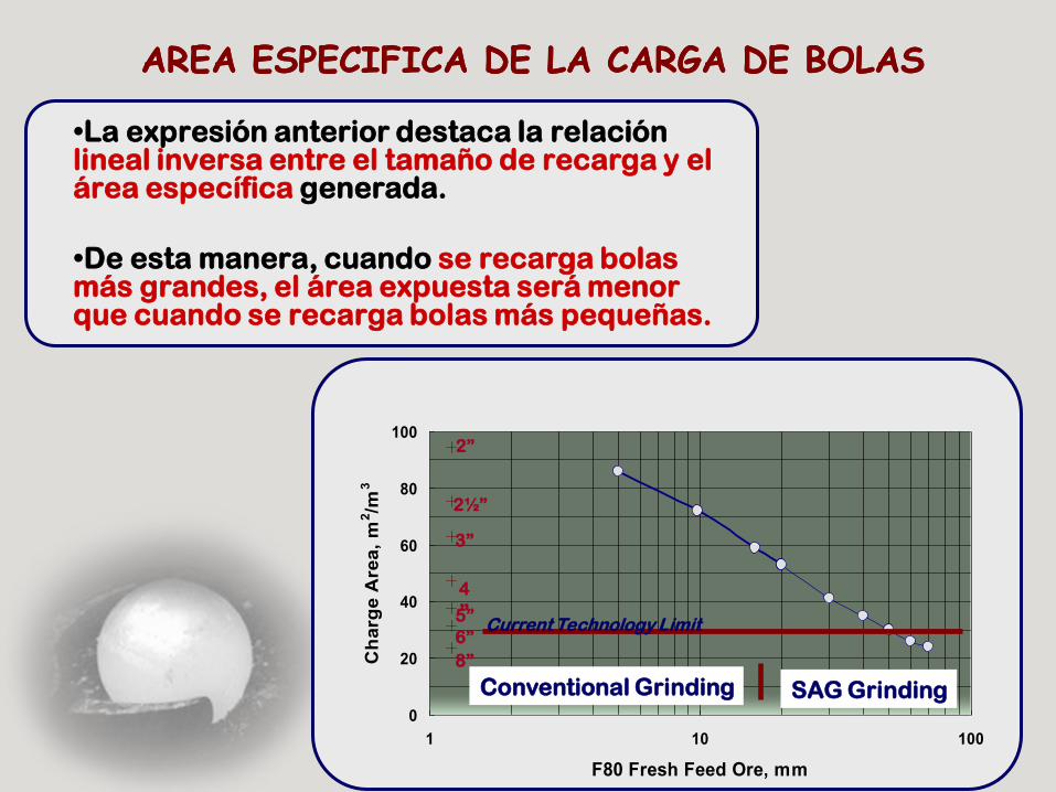
•La expresión anterior destaca la relación lineal inversa entre el tamaño de recarga y el área específica generada.
•De esta manera, cuando se recarga bolas más grandes, el área expuesta será menor que cuando se recarga bolas más pequeñas.
0
20
40
60
80
100
1 10 100
F80 Fresh Feed Ore, mm
Ch
arg
e A
rea
, m
2/m
3
Conventional Grinding SAG Grinding
Current Technology Limit
2”
2½”
3”
4
”5”
6”
8”
AREA ESPECIFICA DE LA CARGA DE BOLASAREA ESPECIFICA DE LA CARGA DE BOLAS
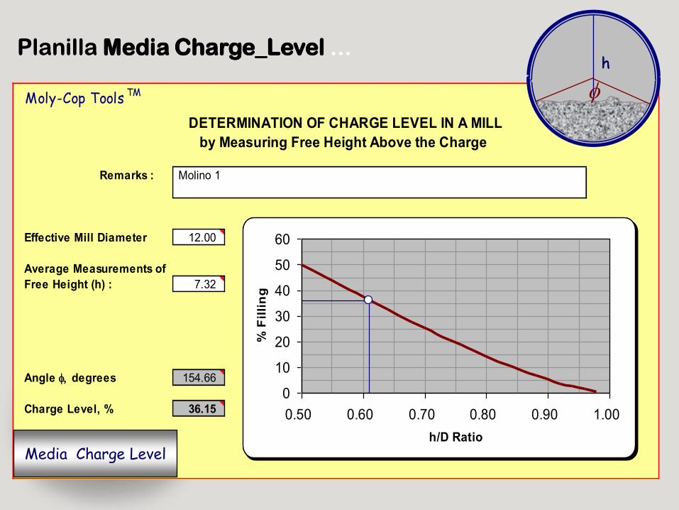
Planilla Planilla Media Charge_LevelMedia Charge_Level ......
Moly-Cop Tools TM
Remarks :
Effective Mill Diameter 12.00
Average Measurements of
Free Height (h) : 7.32
Angle degrees 154.66
Charge Level, % 36.15
by Measuring Free Height Above the Charge
DETERMINATION OF CHARGE LEVEL IN A MILL
Molino 1
0
10
20
30
40
50
60
0.50 0.60 0.70 0.80 0.90 1.00
h/D Ratio
% F
illi
ng
hh
Media Charge Level
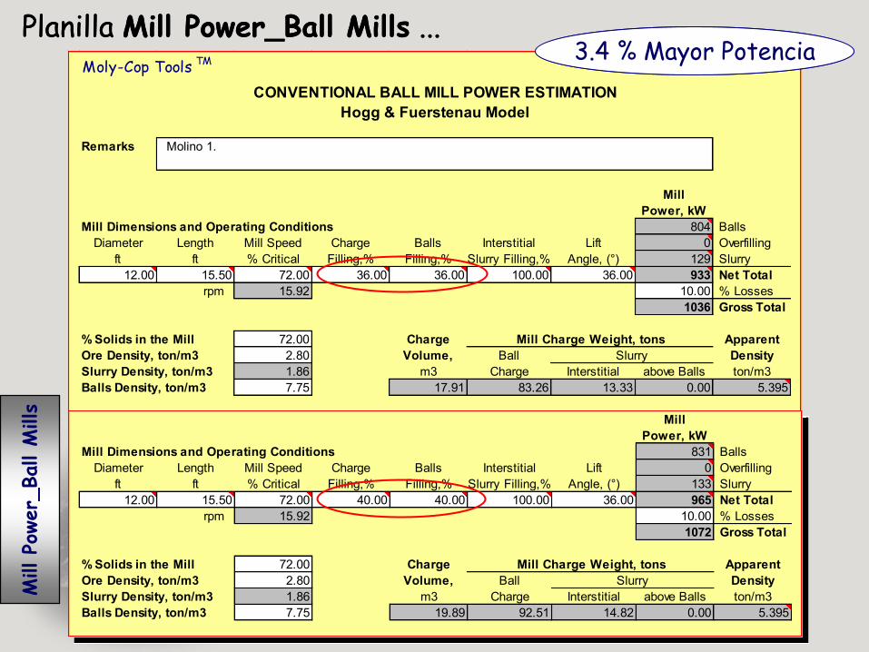
Planilla Planilla Mill Power_Ball MillsMill Power_Ball Mills ......Moly-Cop Tools TM
Remarks Molino 1.
Mill
Power, kW
Mill Dimensions and Operating Conditions 804 Balls
Diameter Length Mill Speed Charge Balls Interstitial Lift 0 Overfilling
ft ft % Critical Filling,% Filling,% Slurry Filling,% Angle, (°) 129 Slurry
12.00 15.50 72.00 36.00 36.00 100.00 36.00 933 Net Total
rpm 15.92 10.00 % Losses
1036 Gross Total
% Solids in the Mill 72.00 Charge Apparent
Ore Density, ton/m3 2.80 Volume, Ball Density
Slurry Density, ton/m3 1.86 m3 Charge Interstitial above Balls ton/m3
Balls Density, ton/m3 7.75 17.91 83.26 13.33 0.00 5.395
Mill Charge Weight, tons
CONVENTIONAL BALL MILL POWER ESTIMATION
Slurry
Hogg & Fuerstenau Model
Moly-Cop Tools TM
Remarks Molino 1.
Mill
Power, kW
Mill Dimensions and Operating Conditions 804 Balls
Diameter Length Mill Speed Charge Balls Interstitial Lift 0 Overfilling
ft ft % Critical Filling,% Filling,% Slurry Filling,% Angle, (°) 129 Slurry
12.00 15.50 72.00 36.00 36.00 100.00 36.00 933 Net Total
rpm 15.92 10.00 % Losses
1036 Gross Total
% Solids in the Mill 72.00 Charge Apparent
Ore Density, ton/m3 2.80 Volume, Ball Density
Slurry Density, ton/m3 1.86 m3 Charge Interstitial above Balls ton/m3
Balls Density, ton/m3 7.75 17.91 83.26 13.33 0.00 5.395
Mill Charge Weight, tons
CONVENTIONAL BALL MILL POWER ESTIMATION
Slurry
Hogg & Fuerstenau Model
Mill
Power, kW
Mill Dimensions and Operating Conditions 831 Balls
Diameter Length Mill Speed Charge Balls Interstitial Lift 0 Overfilling
ft ft % Critical Filling,% Filling,% Slurry Filling,% Angle, (°) 133 Slurry
12.00 15.50 72.00 40.00 40.00 100.00 36.00 965 Net Total
rpm 15.92 10.00 % Losses
1072 Gross Total
% Solids in the Mill 72.00 Charge Apparent
Ore Density, ton/m3 2.80 Volume, Ball Density
Slurry Density, ton/m3 1.86 m3 Charge Interstitial above Balls ton/m3
Balls Density, ton/m3 7.75 19.89 92.51 14.82 0.00 5.395
Mill Charge Weight, tons
Slurry
3.4 % Mayor Potencia3.4 % Mayor PotenciaM
ill Po
wer_
Ball M
ills


Planilla Planilla Bond_Op. Work IndexBond_Op. Work Index ....Caso BaseCaso Base..
Moly-Cop Tools TM
Remarks Molino 1.
GRINDING TASK :
Ore Work Index, kWh/ton (metric) 13.03 Specific Energy, kWh/ton 9.33
Feed Size, F80, microns 9795 Net Power Available, kW 933
Product Size, P80, microns 150.0 Number of Mills for the Task 1
Total Plant Throughput, ton/hr 100.00 Net kW / Mill 933
Mill
MILL DIMENSIONS AND OPERATING CONDITIONS : Power, kW
804 Balls
Diameter Length Mill Speed Charge Balls Interstitial Lift 0 Overfilling
ft ft % Critical Filling,% Filling,% Slurry Filling,% Angle, (°) 129 Slurry
12.00 15.50 72.00 36.00 36.00 100.00 36.00 933 Net Total
L/D rpm 10.0 % Losses
1.29 15.92 1036 Gross Total
% Solids in the Mill 72.00 Charge Apparent
Ore Density, ton/m3 2.80 Volume, Ball Density
Slurry Density, ton/m3 1.86 m3 Charge Interstitial above Balls ton/m3
Balls Density, ton/m3 7.75 17.91 83.26 13.33 0.00 5.395
Mill Charge Weight, tons
BOND'S LAW APPLICATION
Slurry
Estimation of the Operating Work Index from Plant Data
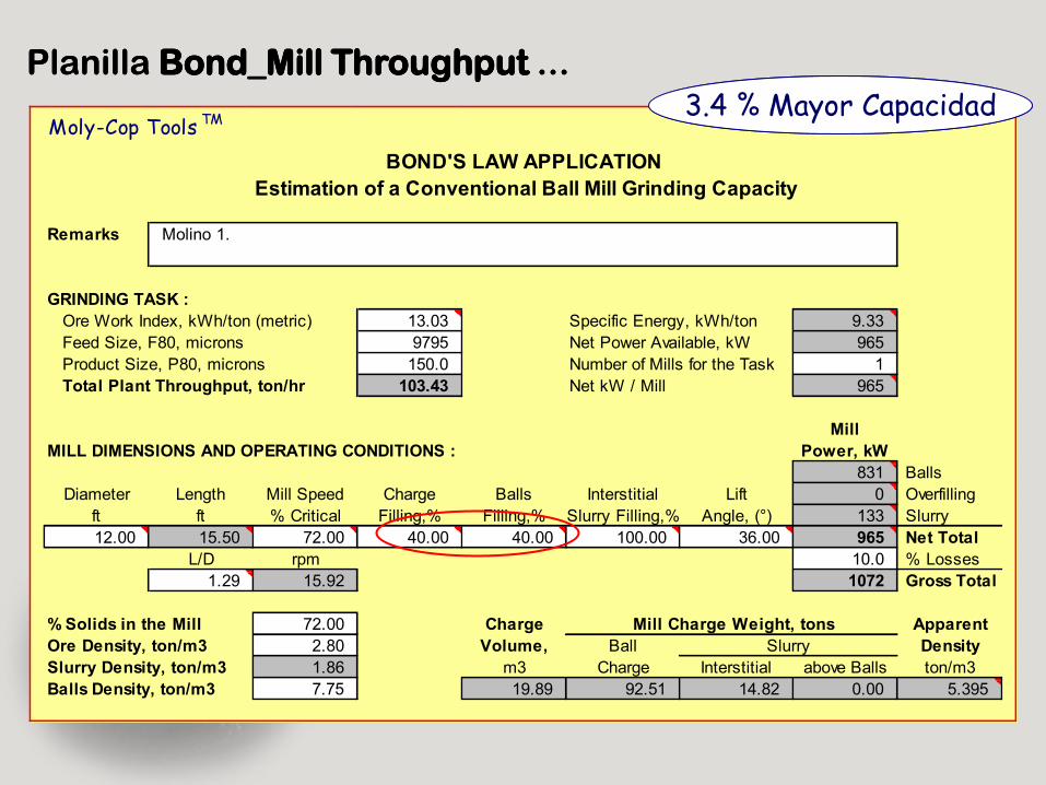
Planilla Planilla Bond_Mill ThroughputBond_Mill Throughput ......
Moly-Cop Tools TM
Remarks Molino 1.
GRINDING TASK :
Ore Work Index, kWh/ton (metric) 13.03 Specific Energy, kWh/ton 9.33
Feed Size, F80, microns 9795 Net Power Available, kW 965
Product Size, P80, microns 150.0 Number of Mills for the Task 1
Total Plant Throughput, ton/hr 103.43 Net kW / Mill 965
Mill
MILL DIMENSIONS AND OPERATING CONDITIONS : Power, kW
831 Balls
Diameter Length Mill Speed Charge Balls Interstitial Lift 0 Overfilling
ft ft % Critical Filling,% Filling,% Slurry Filling,% Angle, (°) 133 Slurry
12.00 15.50 72.00 40.00 40.00 100.00 36.00 965 Net Total
L/D rpm 10.0 % Losses
1.29 15.92 1072 Gross Total
% Solids in the Mill 72.00 Charge Apparent
Ore Density, ton/m3 2.80 Volume, Ball Density
Slurry Density, ton/m3 1.86 m3 Charge Interstitial above Balls ton/m3
Balls Density, ton/m3 7.75 19.89 92.51 14.82 0.00 5.395
Mill Charge Weight, tons
BOND'S LAW APPLICATION
Slurry
Estimation of a Conventional Ball Mill Grinding Capacity
3.4 % Mayor Capacidad3.4 % Mayor Capacidad
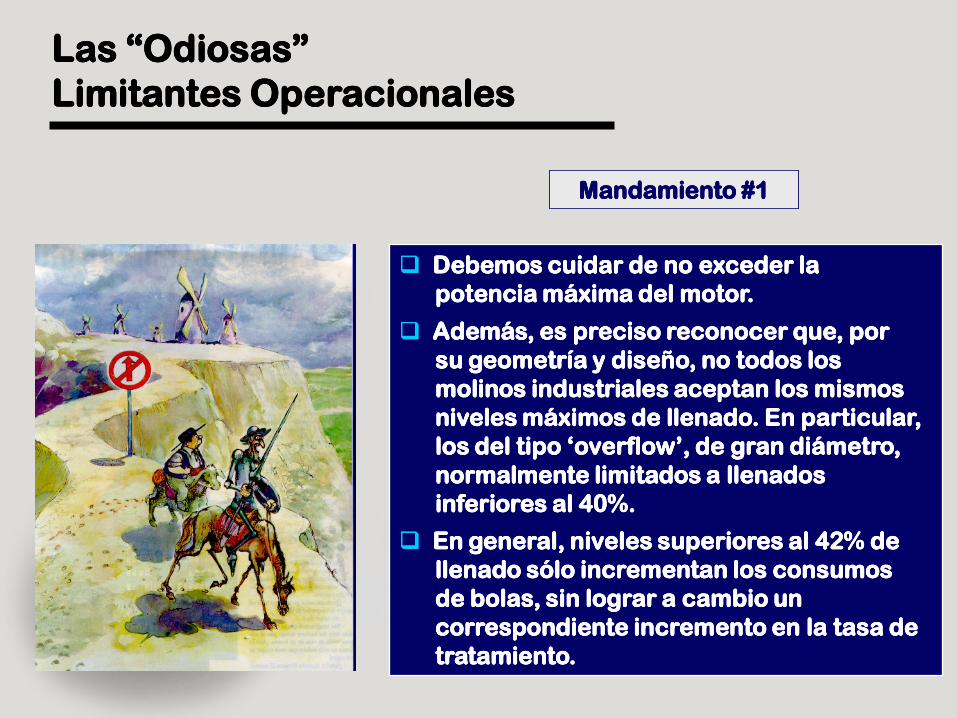
Las “Odiosas”Las “Odiosas”
Limitantes OperacionalesLimitantes Operacionales
Debemos cuidar de no exceder laDebemos cuidar de no exceder la
potencia máxima del motor.potencia máxima del motor.
Además, eAdemás, es preciso reconocer que, pors preciso reconocer que, por
susu geometría y diseño, no todos losgeometría y diseño, no todos los
molinosmolinos industriales aceptan los mismosindustriales aceptan los mismos
nivelesniveles máximosmáximos de llenadode llenado.. EEn particularn particular,,
los del tipo „overflow‟, de gran diámetro,los del tipo „overflow‟, de gran diámetro,
normalmente limitados a llenadosnormalmente limitados a llenados
inferiores al 40%.inferiores al 40%.
En general, niveles superiores al 42% deEn general, niveles superiores al 42% de
llenado sólo incrementan los consumosllenado sólo incrementan los consumos
de bolas, sin lograr a cambio unde bolas, sin lograr a cambio un
correspondiente incremento en la tasa decorrespondiente incremento en la tasa de
tratamiento.tratamiento.
Mandamiento #1Mandamiento #1Mandamiento #1Mandamiento #1

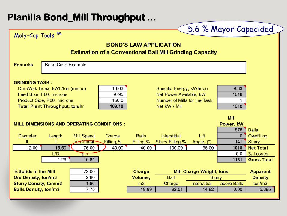
Moly-Cop Tools TM
Remarks Base Case Example
GRINDING TASK :
Ore Work Index, kWh/ton (metric) 13.03 Specific Energy, kWh/ton 9.33
Feed Size, F80, microns 9795 Net Power Available, kW 1018
Product Size, P80, microns 150.0 Number of Mills for the Task 1
Total Plant Throughput, ton/hr 109.18 Net kW / Mill 1018
Mill
MILL DIMENSIONS AND OPERATING CONDITIONS : Power, kW
878 Balls
Diameter Length Mill Speed Charge Balls Interstitial Lift 0 Overfilling
ft ft % Critical Filling,% Filling,% Slurry Filling,% Angle, (°) 141 Slurry
12.00 15.50 76.00 40.00 40.00 100.00 36.00 1018 Net Total
L/D rpm 10.0 % Losses
1.29 16.81 1131 Gross Total
% Solids in the Mill 72.00 Charge Apparent
Ore Density, ton/m3 2.80 Volume, Ball Density
Slurry Density, ton/m3 1.86 m3 Charge Interstitial above Balls ton/m3
Balls Density, ton/m3 7.75 19.89 92.51 14.82 0.00 5.395
Mill Charge Weight, tons
BOND'S LAW APPLICATION
Slurry
Estimation of a Conventional Ball Mill Grinding Capacity
Planilla Planilla Bond_Mill ThroughputBond_Mill Throughput ......
5.6 % Mayor Capacidad5.6 % Mayor Capacidad
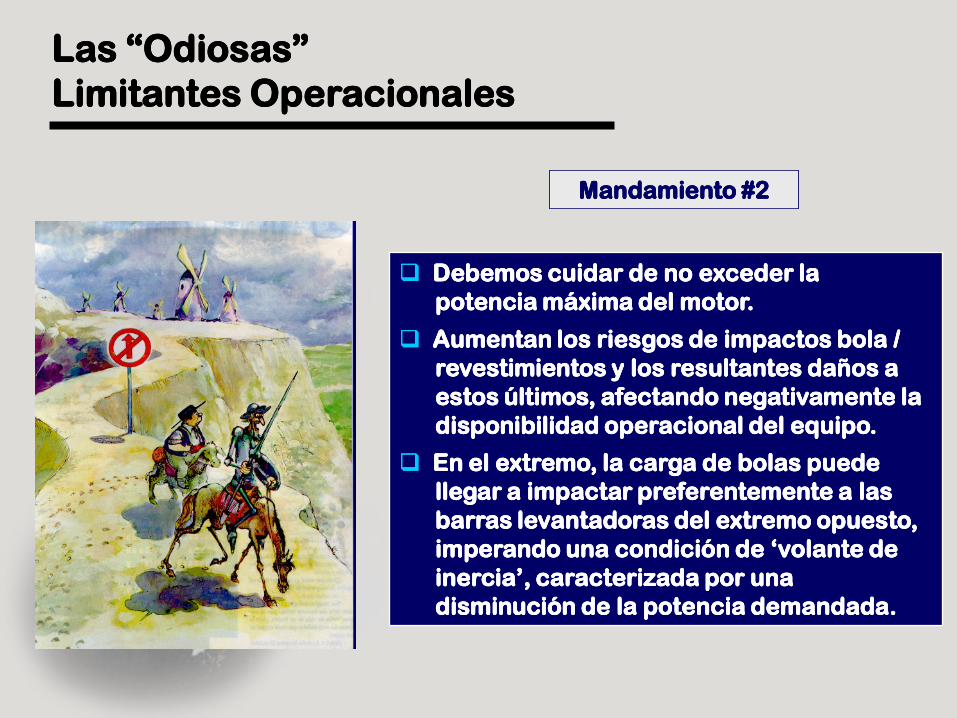
Las “Odiosas”Las “Odiosas”
Limitantes OperacionalesLimitantes Operacionales
Debemos cuidar de no exceder laDebemos cuidar de no exceder la
potencia máxima del motor.potencia máxima del motor.
AAumentan los riesgos de impactos bolaumentan los riesgos de impactos bola //
revestimientorevestimientoss y los resultantes daños ay los resultantes daños a
estos últimos, afectando negativamente laestos últimos, afectando negativamente la
disponibilidad operacional del equipo.disponibilidad operacional del equipo.
En el extremo, la carga de bolas puedeEn el extremo, la carga de bolas puede
llegar a impactar preferentemente a lasllegar a impactar preferentemente a las
barras levantadoras del extremo opuesto,barras levantadoras del extremo opuesto,
imperando una condición de „volante deimperando una condición de „volante de
inercia‟, caracterizada por unainercia‟, caracterizada por una
disminución de la potencia demandada.disminución de la potencia demandada.
Mandamiento #2Mandamiento #2Mandamiento #2Mandamiento #2

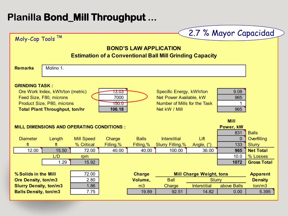
Moly-Cop Tools TM
Remarks Molino 1.
GRINDING TASK :
Ore Work Index, kWh/ton (metric) 13.03 Specific Energy, kWh/ton 9.08
Feed Size, F80, microns 7000 Net Power Available, kW 965
Product Size, P80, microns 150.0 Number of Mills for the Task 1
Total Plant Throughput, ton/hr 106.18 Net kW / Mill 965
Mill
MILL DIMENSIONS AND OPERATING CONDITIONS : Power, kW
831 Balls
Diameter Length Mill Speed Charge Balls Interstitial Lift 0 Overfilling
ft ft % Critical Filling,% Filling,% Slurry Filling,% Angle, (°) 133 Slurry
12.00 15.50 72.00 40.00 40.00 100.00 36.00 965 Net Total
L/D rpm 10.0 % Losses
1.29 15.92 1072 Gross Total
% Solids in the Mill 72.00 Charge Apparent
Ore Density, ton/m3 2.80 Volume, Ball Density
Slurry Density, ton/m3 1.86 m3 Charge Interstitial above Balls ton/m3
Balls Density, ton/m3 7.75 19.89 92.51 14.82 0.00 5.395
Mill Charge Weight, tons
BOND'S LAW APPLICATION
Slurry
Estimation of a Conventional Ball Mill Grinding Capacity
Planilla Planilla Bond_Mill ThroughputBond_Mill Throughput ......
2.7 % Mayor Capacidad2.7 % Mayor Capacidad
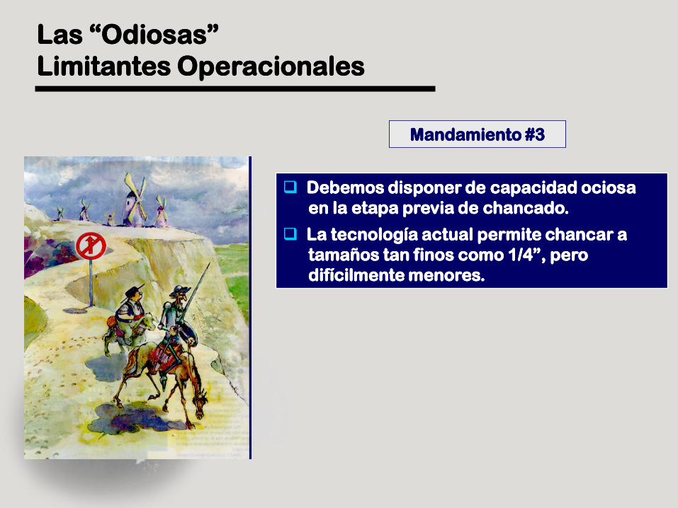
Las “Odiosas”Las “Odiosas”
Limitantes OperacionalesLimitantes Operacionales
Debemos disponer de capacidad ociosaDebemos disponer de capacidad ociosa
en la etapa previa de chancado.en la etapa previa de chancado.
La tecnología actual permite chancar aLa tecnología actual permite chancar a
tamaños tan finos como 1/4”, perotamaños tan finos como 1/4”, pero
difícilmente menores.difícilmente menores.
Mandamiento #3Mandamiento #3Mandamiento #3Mandamiento #3

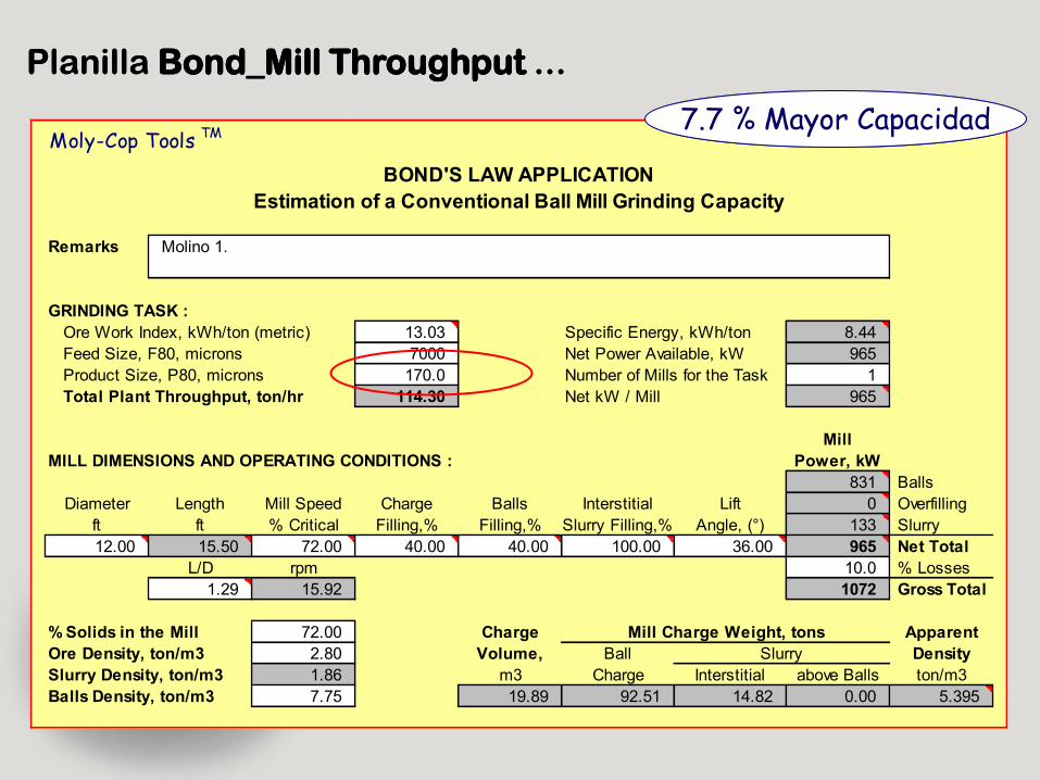
Moly-Cop Tools TM
Remarks Molino 1.
GRINDING TASK :
Ore Work Index, kWh/ton (metric) 13.03 Specific Energy, kWh/ton 8.44
Feed Size, F80, microns 7000 Net Power Available, kW 965
Product Size, P80, microns 170.0 Number of Mills for the Task 1
Total Plant Throughput, ton/hr 114.30 Net kW / Mill 965
Mill
MILL DIMENSIONS AND OPERATING CONDITIONS : Power, kW
831 Balls
Diameter Length Mill Speed Charge Balls Interstitial Lift 0 Overfilling
ft ft % Critical Filling,% Filling,% Slurry Filling,% Angle, (°) 133 Slurry
12.00 15.50 72.00 40.00 40.00 100.00 36.00 965 Net Total
L/D rpm 10.0 % Losses
1.29 15.92 1072 Gross Total
% Solids in the Mill 72.00 Charge Apparent
Ore Density, ton/m3 2.80 Volume, Ball Density
Slurry Density, ton/m3 1.86 m3 Charge Interstitial above Balls ton/m3
Balls Density, ton/m3 7.75 19.89 92.51 14.82 0.00 5.395
Mill Charge Weight, tons
BOND'S LAW APPLICATION
Slurry
Estimation of a Conventional Ball Mill Grinding Capacity
Planilla Planilla Bond_Mill ThroughputBond_Mill Throughput ......
7.7 % Mayor Capacidad7.7 % Mayor Capacidad
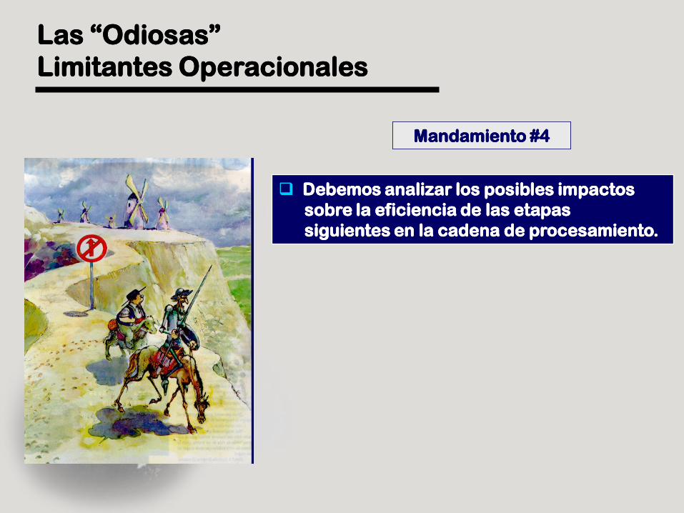
Las “Odiosas”Las “Odiosas”
Limitantes OperacionalesLimitantes Operacionales
Debemos analizar los posibles impactosDebemos analizar los posibles impactos
sobre la eficiencia de las etapassobre la eficiencia de las etapas
siguientes en la cadena de procesamiento.siguientes en la cadena de procesamiento.
Mandamiento #4Mandamiento #4Mandamiento #4Mandamiento #4

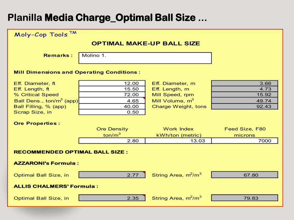
Planilla Planilla Media Charge_Optimal Ball SizeMedia Charge_Optimal Ball Size ......
Moly-Cop Tools TM
Remarks :
Mill Dimensions and Operating Conditions :
Eff. Diameter, ft 12.00 Eff. Diameter, m 3.66
Eff. Length, ft 15.50 Eff. Length, m 4.73
% Critical Speed 72.00 Mill Speed, rpm 15.92
Ball Dens., ton/m3 (app) 4.65 Mill Volume, m3 49.74
Ball Filling, % (app) 40.00 Charge Weight, tons 92.43
Scrap Size, in 0.50
Ore Properties :
Ore Density Work Index Feed Size, F80
ton/m3 kWh/ton (metric) microns
2.80 13.03 7000
RECOMMENDED OPTIMAL BALL SIZE :
AZZARONI's Formula :
Optimal Ball Size, in 2.77 String Area, m2/m3 67.80
ALLIS CHALMERS' Formula :
Optimal Ball Size, in 2.35 String Area, m2/m3 79.83
OPTIMAL MAKE-UP BALL SIZE
Molino 1.
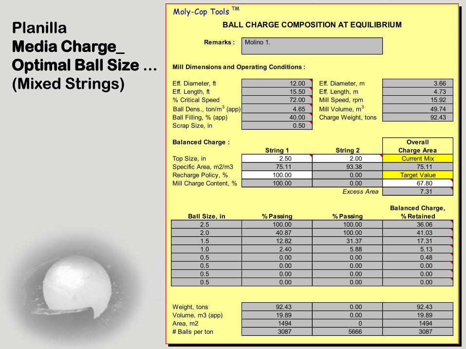
PlanillaPlanilla
Media Charge_Media Charge_
Optimal Ball SizeOptimal Ball Size ......
(Mixed Strings)(Mixed Strings)
Moly-Cop Tools TM
Remarks :
Mill Dimensions and Operating Conditions :
Eff. Diameter, ft 12.00 Eff. Diameter, m 3.66
Eff. Length, ft 15.50 Eff. Length, m 4.73
% Critical Speed 72.00 Mill Speed, rpm 15.92
Ball Dens., ton/m3 (app) 4.65 Mill Volume, m3 49.74
Ball Filling, % (app) 40.00 Charge Weight, tons 92.43
Scrap Size, in 0.50
Balanced Charge : Overall
String 1 String 2 Charge Area
Top Size, in 2.50 2.00 Current Mix
Specific Area, m2/m3 75.11 93.38 75.11
Recharge Policy, % 100.00 0.00 Target Value
Mill Charge Content, % 100.00 0.00 67.80
Excess Area 7.31
Balanced Charge,
Ball Size, in % Passing % Passing % Retained
2.5 100.00 100.00 36.06
2.0 40.87 100.00 41.03
1.5 12.82 31.37 17.31
1.0 2.40 5.88 5.13
0.5 0.00 0.00 0.48
0.5 0.00 0.00 0.00
0.5 0.00 0.00 0.00
0.5 0.00 0.00 0.00
Weight, tons 92.43 0.00 92.43
Volume, m3 (app) 19.89 0.00 19.89
Area, m2 1494 0 1494
# Balls per ton 3087 5666 3087
BALL CHARGE COMPOSITION AT EQUILIBRIUM
Molino 1.
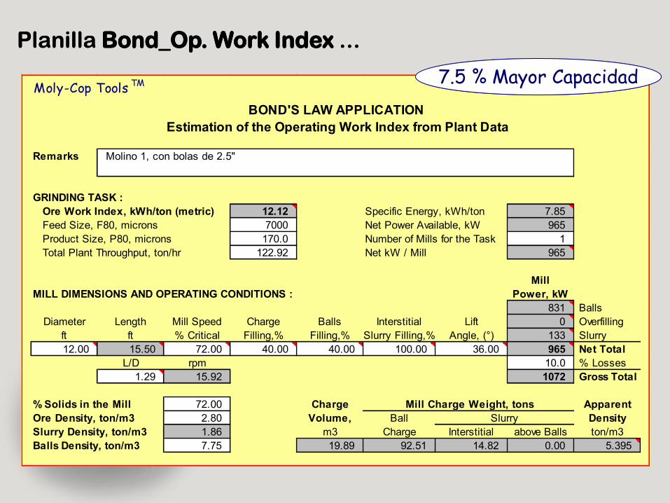
Planilla Planilla Bond_Op. Work IndexBond_Op. Work Index ......
Moly-Cop Tools TM
Remarks Molino 1, con bolas de 2.5"
GRINDING TASK :
Ore Work Index, kWh/ton (metric) 12.12 Specific Energy, kWh/ton 7.85
Feed Size, F80, microns 7000 Net Power Available, kW 965
Product Size, P80, microns 170.0 Number of Mills for the Task 1
Total Plant Throughput, ton/hr 122.92 Net kW / Mill 965
Mill
MILL DIMENSIONS AND OPERATING CONDITIONS : Power, kW
831 Balls
Diameter Length Mill Speed Charge Balls Interstitial Lift 0 Overfilling
ft ft % Critical Filling,% Filling,% Slurry Filling,% Angle, (°) 133 Slurry
12.00 15.50 72.00 40.00 40.00 100.00 36.00 965 Net Total
L/D rpm 10.0 % Losses
1.29 15.92 1072 Gross Total
% Solids in the Mill 72.00 Charge Apparent
Ore Density, ton/m3 2.80 Volume, Ball Density
Slurry Density, ton/m3 1.86 m3 Charge Interstitial above Balls ton/m3
Balls Density, ton/m3 7.75 19.89 92.51 14.82 0.00 5.395
Mill Charge Weight, tons
BOND'S LAW APPLICATION
Slurry
Estimation of the Operating Work Index from Plant Data
7.5 % Mayor Capacidad7.5 % Mayor Capacidad

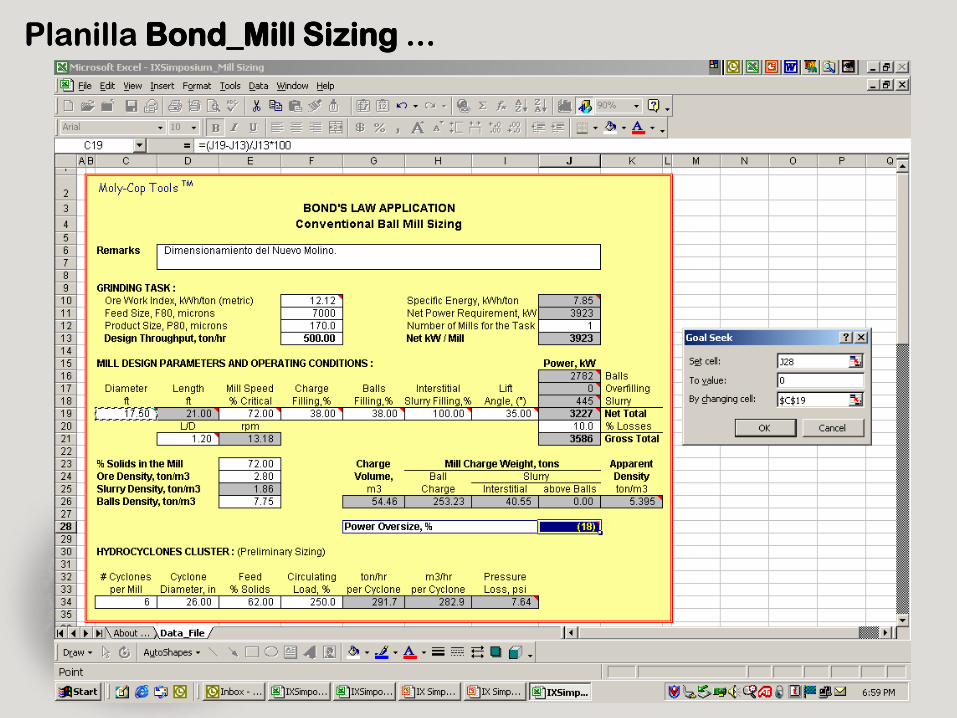
Planilla Planilla Bond_Mill SizingBond_Mill Sizing ......
Moly-Cop Tools TM
Remarks Dimensionamiento del Nuevo Molino.
GRINDING TASK :
Ore Work Index, kWh/ton (metric) 12.12 Specific Energy, kWh/ton 7.85
Feed Size, F80, microns 7000 Net Power Requirement, kW 3923
Product Size, P80, microns 170.0 Number of Mills for the Task 1
Design Throughput, ton/hr 500.00 Net kW / Mill 3923
MILL DESIGN PARAMETERS AND OPERATING CONDITIONS : Power, kW
2782 Balls
Diameter Length Mill Speed Charge Balls Interstitial Lift 0 Overfilling
ft ft % Critical Filling,% Filling,% Slurry Filling,% Angle, (°) 445 Slurry
17.50 21.00 72.00 38.00 38.00 100.00 35.00 3227 Net Total
L/D rpm 10.0 % Losses
1.20 13.18 3586 Gross Total
% Solids in the Mill 72.00 Charge Apparent
Ore Density, ton/m3 2.80 Volume, Ball Density
Slurry Density, ton/m3 1.86 m3 Charge Interstitial above Balls ton/m3
Balls Density, ton/m3 7.75 54.46 253.23 40.55 0.00 5.395
Power Oversize, % (18)
HYDROCYCLONES CLUSTER : (Preliminary Sizing)
# Cyclones Cyclone Feed Circulating ton/hr m3/hr Pressure
per Mill Diameter, in % Solids Load, % per Cyclone per Cyclone Loss, psi
4 26.00 62.00 250.0 437.5 424.4 17.93
Mill Charge Weight, tons
BOND'S LAW APPLICATION
Slurry
Conventional Ball Mill Sizing
May be set to any May be set to any May be set to any May be set to any
desired value, desired value,
using Tools / Goal using Tools / Goal
Seek, changing Seek, changing
Cell C19Cell C19 or or Cell Cell
D21D21..
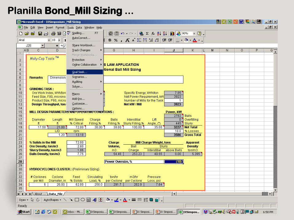
Planilla Planilla Bond_Mill SizingBond_Mill Sizing ......
Planilla Planilla Bond_Mill SizingBond_Mill Sizing ......
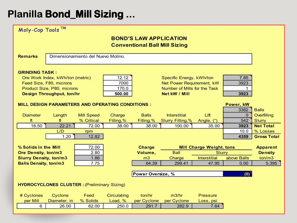
Planilla Planilla Bond_Mill SizingBond_Mill Sizing ......
Moly-Cop Tools TM
Remarks Dimensionamiento del Nuevo Molino.
GRINDING TASK :
Ore Work Index, kWh/ton (metric) 12.12 Specific Energy, kWh/ton 7.85
Feed Size, F80, microns 7000 Net Power Requirement, kW 3923
Product Size, P80, microns 170.0 Number of Mills for the Task 1
Design Throughput, ton/hr 500.00 Net kW / Mill 3923
MILL DESIGN PARAMETERS AND OPERATING CONDITIONS : Power, kW
3382 Balls
Diameter Length Mill Speed Charge Balls Interstitial Lift 0 Overfilling
ft ft % Critical Filling,% Filling,% Slurry Filling,% Angle, (°) 542 Slurry
18.50 22.21 72.00 38.00 38.00 100.00 35.00 3923 Net Total
L/D rpm 10.0 % Losses
1.20 12.82 4359 Gross Total
% Solids in the Mill 72.00 Charge Apparent
Ore Density, ton/m3 2.80 Volume, Ball Density
Slurry Density, ton/m3 1.86 m3 Charge Interstitial above Balls ton/m3
Balls Density, ton/m3 7.75 64.39 299.41 47.95 0.00 5.395
Power Oversize, % (0)
HYDROCYCLONES CLUSTER : (Preliminary Sizing)
# Cyclones Cyclone Feed Circulating ton/hr m3/hr Pressure
per Mill Diameter, in % Solids Load, % per Cyclone per Cyclone Loss, psi
6 26.00 62.00 250.0 291.7 282.9 7.64
Mill Charge Weight, tons
BOND'S LAW APPLICATION
Slurry
Conventional Ball Mill Sizing

Developed by Moly-Cop Grinding SystemsS
ett
ing
Ne
w S
tan
da
rd M
eth
od
olo
gie
s in
Se
ttin
g N
ew
Sta
nd
ard
Me
tho
do
log
ies
in
Gri
nd
ing
Pro
ce
ss
An
aly
sis
Gri
nd
ing
Pro
ce
ss
An
aly
sis

Water ?
La Ley de BondLa Ley de Bond
Es suficiente…??Es suficiente…??
170 tph
Apex ?
# of Cyclones ?
P80 = 150 mm
Vortex ?
CargaCirculante
1833 kW
F80 = 10500 mm
Distribución de producto
Moly-Cop Tools TM : Theoretical Framework
Water
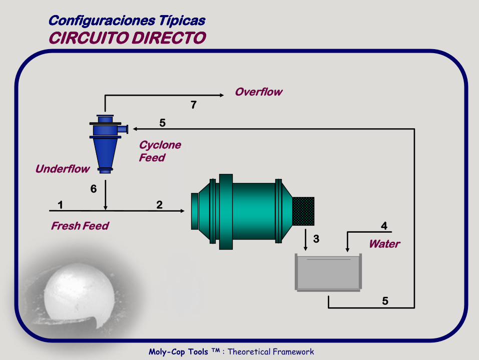
Configuraciones TípicasConfiguraciones Típicas
CIRCUITO DIRECTOCIRCUITO DIRECTO
Fresh Feed
Underflow
CycloneFeed
Overflow
4
3
2
5
7
6
1
5
Moly-Cop Tools TM : Theoretical Framework
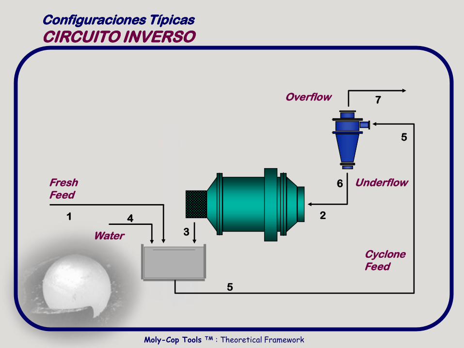
Water
FreshFeed
Underflow
CycloneFeed
Overflow
4
3
2
5
7
6
1
5
Configuraciones TípicasConfiguraciones Típicas
CIRCUITO INVERSOCIRCUITO INVERSO
Moly-Cop Tools TM : Theoretical Framework
Moly-Cop Tools TM : Theoretical Framework
El Proceso de Clasificación
Se denomina clasificación a la operación de separación de los
componentes de una mezcla de partículas en dos o mas fracciones
de acuerdo a su tamaño.
La clasificación en algunos casos es una operación primordial,
especialmente cuando se requieren especificaciones estrictas de
tamaño. En otros casos es una operación auxiliar de la molienda,
donde sus objetivos son asegurar el tamaño de partícula este bajo
un determinado tamaño.
El hidrociclón es sin lugar a dudas el tipo de clasificador mas
ampliamente usado en los circuitos industriales de molienda.

Moly-Cop Tools TM : Theoretical Framework
Modelos de Clasificación con Hidrociclones
Eficiencia de Clasificación,
se denomina como la
fracción de tamaño en la
alimentación que es
recuperada en la descarga.
Se espera que alcance su
mas alto valor para las
partículas gruesas en la
alimentación y que el
contenido de partículas
finas sea mínimo
Moly-Cop Tools TM : Theoretical Framework
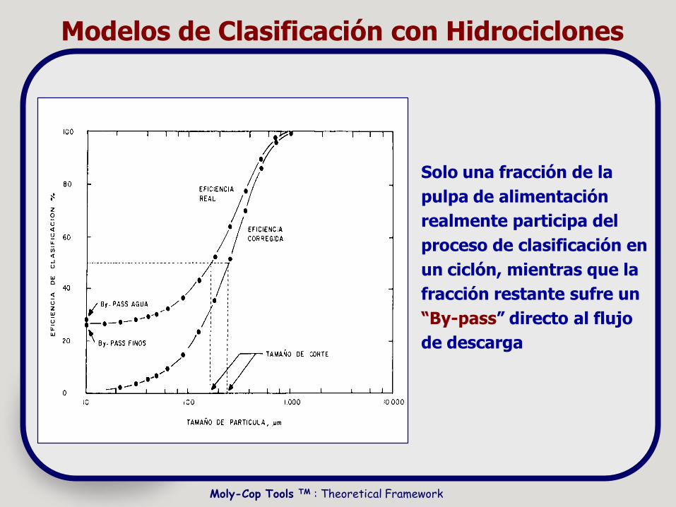
Modelos de Clasificación con Hidrociclones
Solo una fracción de la
pulpa de alimentación
realmente participa del
proceso de clasificación en
un ciclón, mientras que la
fracción restante sufre un
“By-pass” directo al flujo
de descarga
Moly-Cop Tools TM : Theoretical Framework
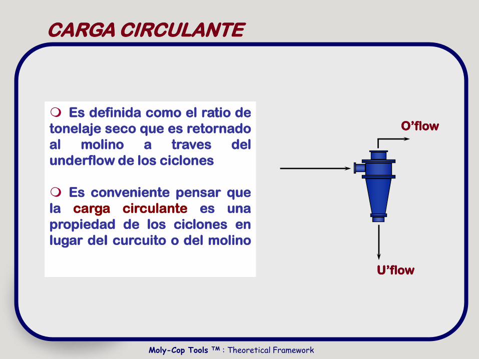
Es definida como el ratio de
tonelaje seco que es retornado
al molino a traves del
underflow de los ciclones
Es conveniente pensar que
la carga circulante es una
propiedad de los ciclones en
lugar deI curcuito o del molino
Es definida como el ratio de
tonelaje seco que es retornado
al molino a traves del
underflow de los ciclones
Es conveniente pensar que
la carga circulante es una
propiedad de los ciclones en
lugar deI curcuito o del molino
CARGA CIRCULANTECARGA CIRCULANTE
O‟flowO‟flow
U‟flowU‟flow
Moly-Cop Tools TM : Theoretical Framework
Modelos empíricos de clasificación
Hasta este momento, el desarrollo en el área de
modelaje matemático ha provenido fundamentalmente de
dos grupos de investigadores encabezados por Lynch y
Plitt y mas recientemente estudios llevados a cabo por J.
L. Bouso y el CIMM de Chile.
Por su parte el CIMM de Chile, desarrollo a partir del
modelo de Plitt ensayos adicionales (77 en total), que
permitieron obtener un modelo de clasificación muy
cercano en su forma al propuesto por Plitt, por lo cual se le
escogió como base para realizar las simulaciones en el
presente trabajo
Moly-Cop Tools TM : Theoretical Framework
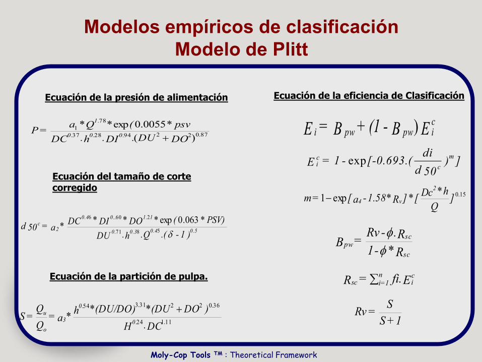
Modelos empíricos de clasificación
Modelo de Plitt
Ecuación de la presión de alimentación
87.022942837
78
1
)(
*0055.0exp**
DODU.DI.h.DC
psv(Qa=P
0.0.0.
1.
Ecuación del tamaño de corte corregido
)1-.(Q.h.DU
PSV)(DODIDC*a=50d
0.50.40.30.
11.0.0.4
2c
5871
260.6 *063.0exp***
Ecuación de la partición de pulpa.
DC.H
)DO(DU)(DU/DOh*a=
Q
Q=S
0.
0.
3
o
u
11.124
36.02231.354 **
EB-(1+B=Ecipwpwi )
ic
c
mE = 1 - [-0.693.(
di
d 50) ]exp
15.0***exp1 ]
Q
hDc[]R1.58-a[=m
2
v4
R-1
R.-Rv=B
sc
scpw
*
1+S
S=Rv
sc i=1n
ic
R = fi.E
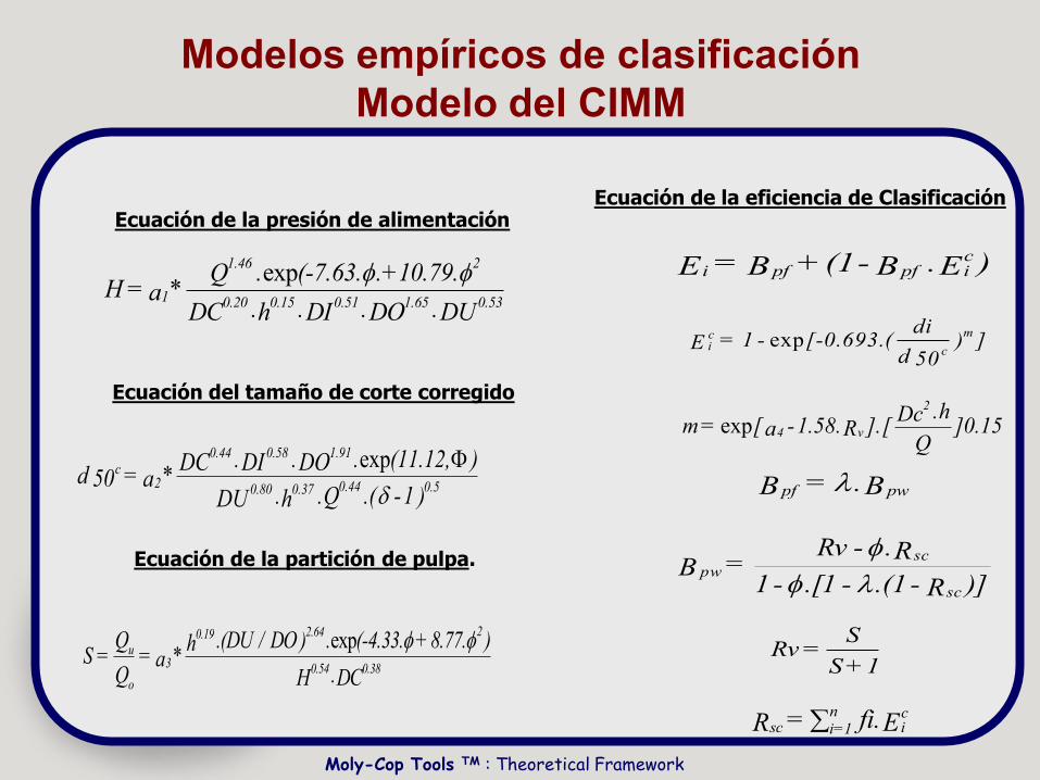
Ecuación de la eficiencia de Clasificación
Moly-Cop Tools TM : Theoretical Framework
Modelos empíricos de clasificación
Modelo del CIMM
i pf pf ic
E = B +(1- B .E )
ic
c
mE = 1 - [-0.693.(
di
d 50) ]exp
m= [a -1.58.R ].[Dc .h
Q]0.154 v
2
exp
pf pwB = .B
)]R-.(1-.[1-1
R.-Rv=B
sc
scpw
Rv=S
S+1
sc i=1n
ic
R = fi.E
Ecuación de la eficiencia de ClasificaciónEcuación de la presión de alimentación
H=a *Q . (-7.63. .+10.79.
DC .h .DI .DO .DU1
1.46 2
0.20 0.15 0.51 1.65 0.53
exp
Ecuación del tamaño de corte corregido
d 50 = a *DC .DI .DO . (11.12, )
DU .h .Q .( -1 )
c2
0.44 0.58 1.91
0.80 0.37 0.44 0.5
exp
S =Q
Q= a *
h .(DU / DO ) . (-4.33. +8.77. )
H .DC
u
o
3
0.19 2.64 2
0.54 0.38
exp
Ecuación de la partición de pulpa.
Moly-Cop Tools TM : Theoretical Framework
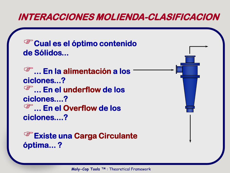
INTERACCIONES MOLIENDAINTERACCIONES MOLIENDA--CLASIFICACIONCLASIFICACION
Cual es el óptimo contenido
de Sólidos...
... En la alimentación a los
ciclones...?
... En el underflow de los
ciclones....?
... En el Overflow de los
ciclones....?
Existe una Carga Circulante
óptima... ?
Moly-Cop Tools TM : Theoretical Framework
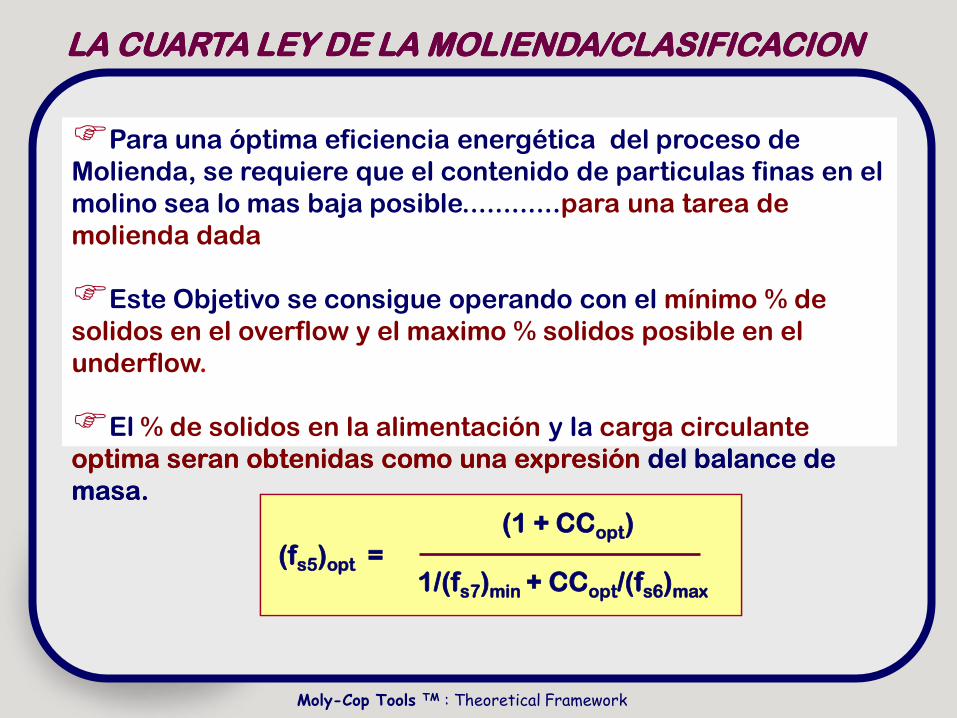
LA CUARTA LEY DE LA MOLIENDA/CLASIFICACIONLA CUARTA LEY DE LA MOLIENDA/CLASIFICACION
Para una óptima eficiencia energética del proceso de
Molienda, se requiere que el contenido de particulas finas en el
molino sea lo mas baja posible............para una tarea de
molienda dada
Este Objetivo se consigue operando con el mínimo % de
solidos en el overflow y el maximo % solidos posible en el
underflow.
El % de solidos en la alimentación y la carga circulante
optima seran obtenidas como una expresión del balance de
masa.
(fs5)opt =
(1 + CCopt)
1/(fs7)min + CCopt/(fs6)max
Moly-Cop Tools TM : Theoretical Framework
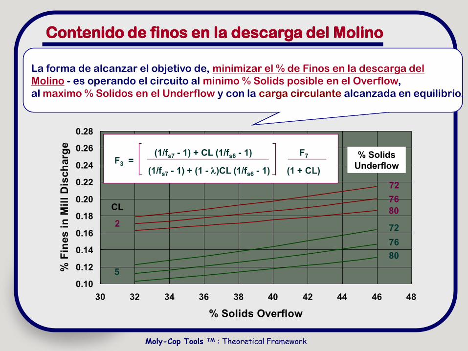
Contenido de finos en la descarga del MolinoContenido de finos en la descarga del Molino
0.10
0.12
0.14
0.16
0.18
0.20
0.22
0.24
0.26
0.28
30 32 34 36 38 40 42 44 46 48
% Solids Overflow
% F
ine
s i
n M
ill
Dis
ch
arg
e
F3 =(1/fs7 - 1) + CL (1/fs6 - 1)
(1/fs7 - 1) + (1 - )CL (1/fs6 - 1)
F7
(1 + CL)
% Solids
Underflow
72
76
80
72
76
80
CL
2
5
alcanzada en equilibrio.
La forma de alcanzar el objetivo de, minimizar el % de Finos en la descarga del
Molino - es operando el circuito al minimo % Solids posible en el Overflow,
al maximo % Solidos en el Underflow y con la carga circulante alcanzada en equilibrio.
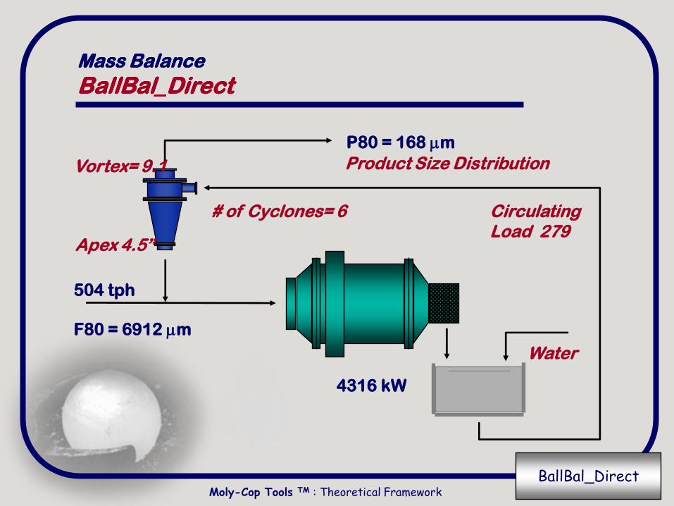
Water
Mass BalanceMass Balance
BallBal_DirectBallBal_Direct
504 tph
Apex 4.5”
# of Cyclones= 6
P80 = 168 mm
Vortex= 9.1
CirculatingLoad 279
4316 kW
F80 = 6912 mm
Product Size Distribution
Moly-Cop Tools TM : Theoretical FrameworkBallBal_Direct

Theoretical FrameworkTheoretical Framework
BATCH PROCEDUREBATCH PROCEDURE
Se
ttin
g N
ew
Sta
nd
ard
Me
tho
do
log
ies
in
Se
ttin
g N
ew
Sta
nd
ard
Me
tho
do
log
ies
in
Gri
nd
ing
Pro
ce
ss
An
aly
sis
Gri
nd
ing
Pro
ce
ss
An
aly
sis
Developed by Moly-Cop Grinding Systems

Moly-Cop Tools TM : Theoretical Framework
Descripción y Muestreos a Nivel Industrial
Condiciones Iniciales
• Molino 16’ x 20’• Nc : 38%• Vc : 73%• Hp : 2600• Bolas 3.5”:2,5” (75:25)• Ciclones D26 (5)•Tm/hr : 290• CC : 360%• D50 : 190 micrones•By pass : 23%
Moly-Cop Tools TM : Theoretical Framework
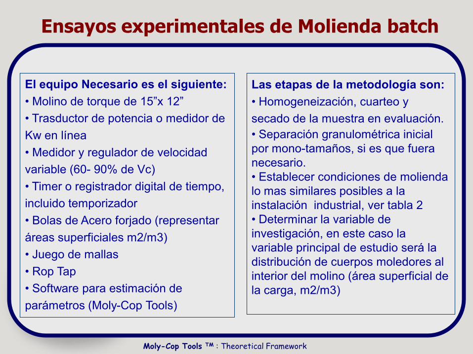
Ensayos experimentales de Molienda batch
El equipo Necesario es el siguiente:
• Molino de torque de 15”x 12”
• Trasductor de potencia o medidor de
Kw en línea
• Medidor y regulador de velocidad
variable (60- 90% de Vc)
• Timer o registrador digital de tiempo,
incluido temporizador
• Bolas de Acero forjado (representar
áreas superficiales m2/m3)
• Juego de mallas
• Rop Tap
• Software para estimación de
parámetros (Moly-Cop Tools)
Las etapas de la metodología son:
• Homogeneización, cuarteo y
secado de la muestra en evaluación.
• Separación granulométrica inicial
por mono-tamaños, si es que fuera
necesario.
• Establecer condiciones de molienda
lo mas similares posibles a la
instalación industrial, ver tabla 2
• Determinar la variable de
investigación, en este caso la
variable principal de estudio será la
distribución de cuerpos moledores al
interior del molino (área superficial de
la carga, m2/m3)

Moly-Cop Tools TM : Theoretical Framework
Metodología de experimentaciónCondiciones de Molienda
Variable Unidad Valor
Tamaño de Alimentación (% -1/2”) 83
% de sólidos % 75
Nivel de llenado de carga % 38
Llenado intersticial % 40
Velocidad del molino Rpm 50
Velocidad crítica % 73
Tiempos de molienda Min 2,4
Alimentación a molino Kg 7.5
Carga de bolas Kg 21.0

Moly-Cop Tools TM : Theoretical Framework
Metodología de experimentaciónCondiciones de Molienda
Monofracción Collar Evaluado Tiempo de Mol.
+ 3/8" 3.5", 3.0" 2 y 4 min
-3/8", + 6" 3.5", 3.0",2.5' "
-6, + 20 2.0", 2.5" "
Alimentación Collar Evaluado
Area
Superficial
m2/m3
Tiempo de
Molienda
Representativa 3.5" 49.0 2 y 4 min
" 3.0" 58.0 "
" 2.5" 70.0 "
" 2.0" 86.0 "

Theoretical FrameworkTheoretical Framework
MODELO GENERAL DE LA MOLIENDAMODELO GENERAL DE LA MOLIENDA
Se
ttin
g N
ew
Sta
nd
ard
Me
tho
do
log
ies
in
Se
ttin
g N
ew
Sta
nd
ard
Me
tho
do
log
ies
in
Gri
nd
ing
Pro
ce
ss
An
aly
sis
Gri
nd
ing
Pro
ce
ss
An
aly
sis
Developed by Moly-Cop Grinding Systems

Moly-Cop Tools TM : Theoretical Framework
(1-S1Dt) f1
S1Dt f1
b21S1Dt f1
bi1S1Dt f1
bn1S1Dt f1
(1-S2Dt) f2
S2Dt f2
bi2S2Dt f2
bn2S2Dt f2
t = t
f1
f2
fi
fn
2
3
i + 1
n + 1
t = t + Dt
2
3
i + 1
n + 1
Caracterización Cinetica de la MoliendaCaracterización Cinetica de la Molienda
Moly-Cop Tools TM : Theoretical Framework
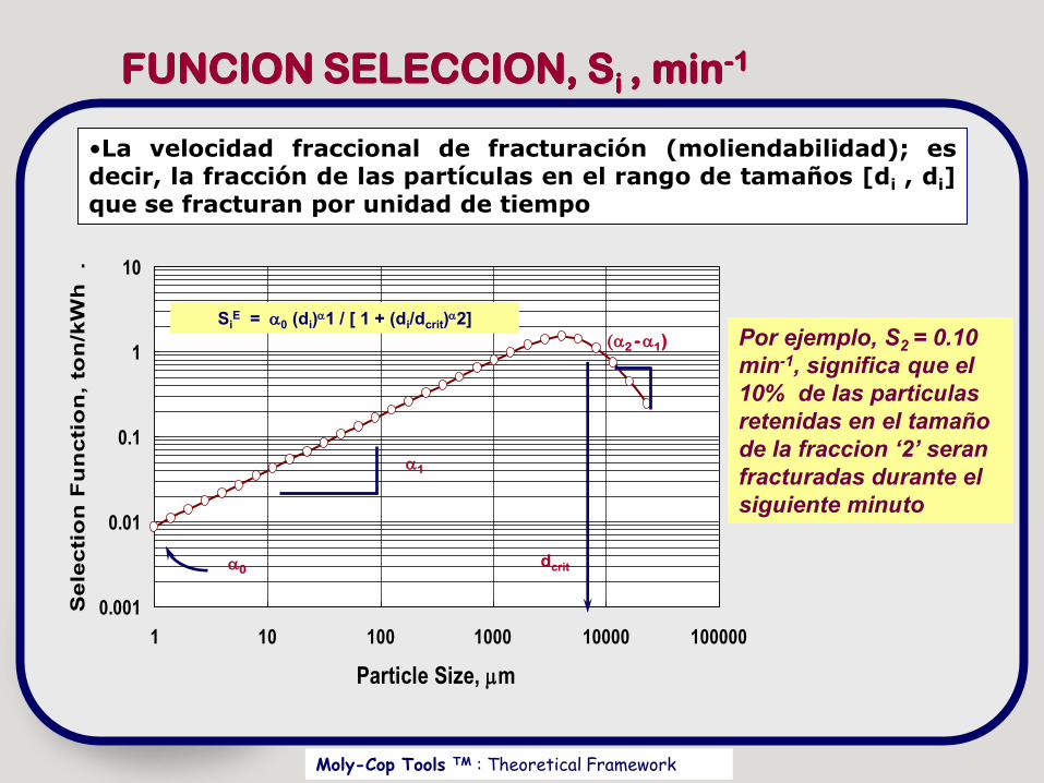
FUNCION SELECCION, SFUNCION SELECCION, Si i , min, min--11
Por ejemplo, S2 = 0.10
min-1, significa que el
10% de las particulas
retenidas en el tamaño
de la fraccion ‘2’ seran
fracturadas durante el
siguiente minuto
Por ejemplo, S2 = 0.10
min-1, significa que el
10% de las particulas
retenidas en el tamaño
de la fraccion ‘2’ seran
fracturadas durante el
siguiente minuto
•La velocidad fraccional de fracturación (moliendabilidad); esdecir, la fracción de las partículas en el rango de tamaños [di , di]que se fracturan por unidad de tiempo
0.001
0.01
0.1
1
10
1 10 100 1000 10000 100000
Particle Size, mm
Sele
cti
on
Fu
ncti
on
, to
n/k
Wh
.
SiE = 0 (di)
1 / [ 1 + (di/dcrit)2]Si
E = 0 (di)1 / [ 1 + (di/dcrit)
2]
0
1
dcrit
(2 -1)
Moly-Cop Tools TM : Theoretical Framework
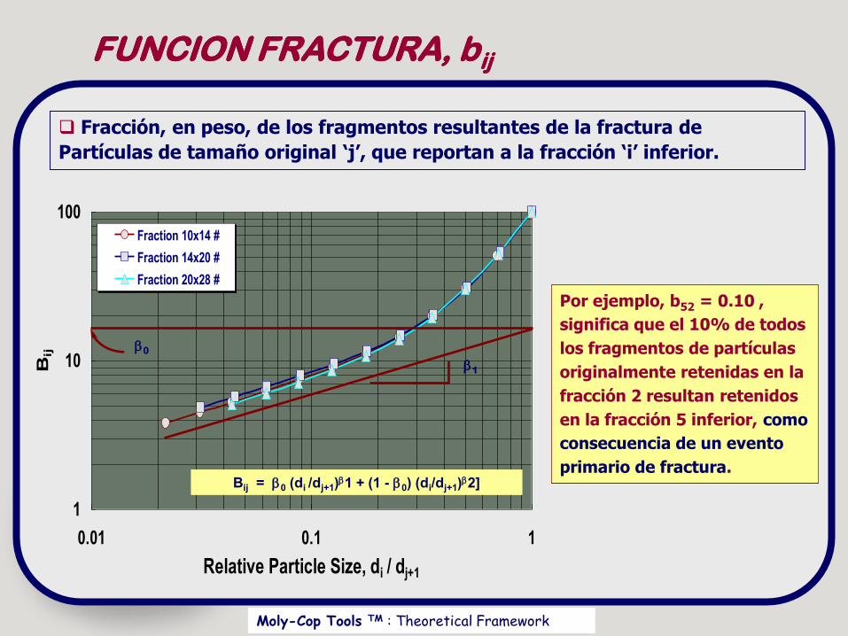
FUNCION FRACTURA, bFUNCION FRACTURA, bijij
Fracción, en peso, de los fragmentos resultantes de la fractura de
Partículas de tamaño original „j‟, que reportan a la fracción „i‟ inferior.
Por ejemplo, b
significa que el 10% de todos
los fragmentos de partículas
originalmente retenidas en la
fracción 2 resultan retenidos
en la fracción 5 inferior, como
consecuencia de un evento
primario de fractura
Por ejemplo, b52 = 0.10 ,
significa que el 10% de todos
los fragmentos de partículas
originalmente retenidas en la
fracción 2 resultan retenidos
en la fracción 5 inferior, como
consecuencia de un evento
primario de fractura.
1
10
100
0.01 0.1 1
Relative Particle Size, di / dj+1
Bij
Fraction 10x14 #
Fraction 14x20 #
Fraction 20x28 #
Bij = b0 (di /dj+1)b1 + (1 - b0) (di/dj+1)
b2]Bij = b0 (di /dj+1)b1 + (1 - b0) (di/dj+1)
b2]
b0
b1
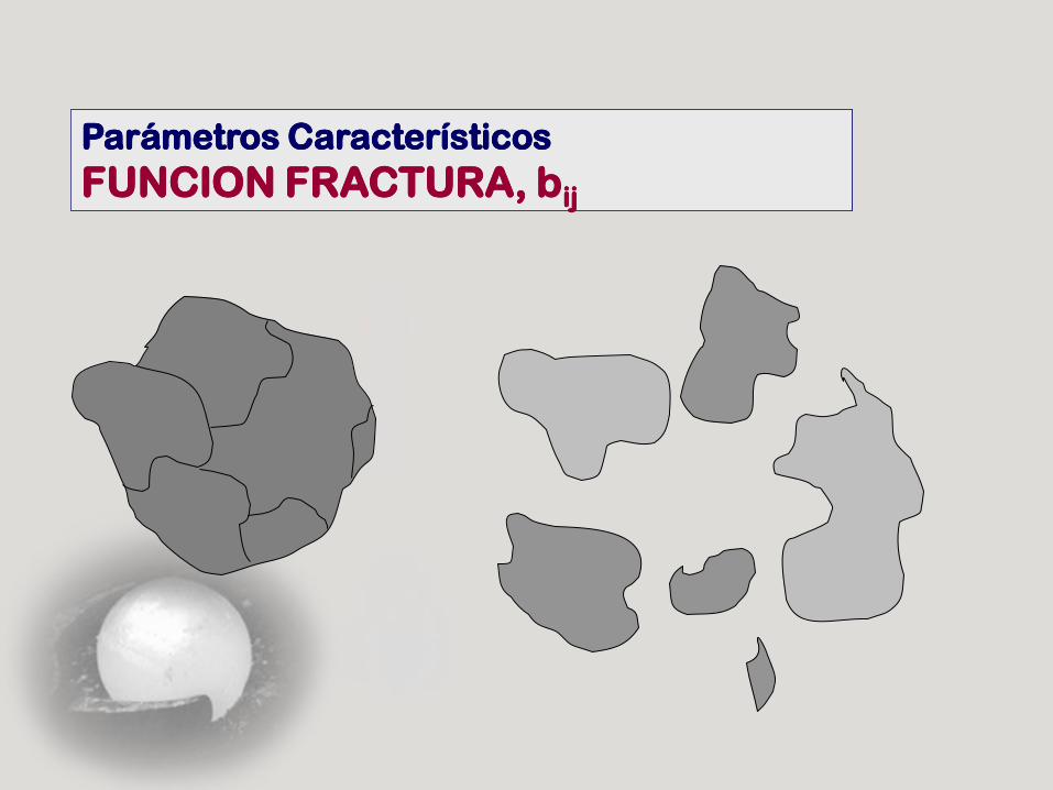
Parámetros CaracterísticosParámetros Característicos
FUNCION FRACTURA, bFUNCION FRACTURA, bParámetros CaracterísticosParámetros Característicos
FUNCION FRACTURA, bFUNCION FRACTURA, bijij
Moly-Cop Tools TM : Theoretical Framework
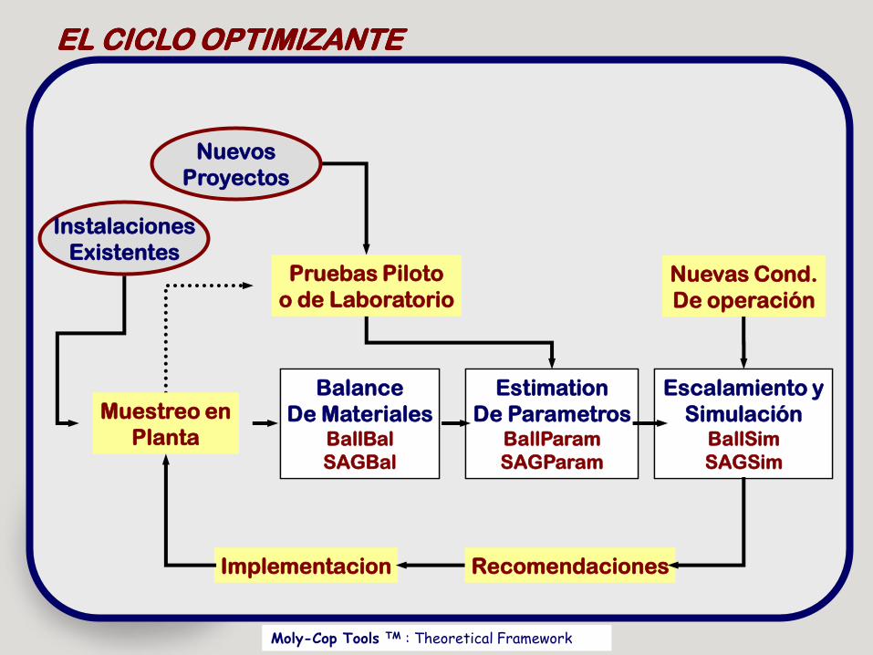
EL CICLO OPTIMIZANTEEL CICLO OPTIMIZANTE
Balance
De Materiales
Balance
De MaterialesBallBal
SAGBal
Estimation
De Parametros
Estimation
De ParametrosBallParam
SAGParam
Escalamiento yEscalamiento y
SimulaciónBallSim
SAGSim
Nuevas Cond.
De operación
Nuevas Cond.
De operación
Nuevos
Proyectos
Pruebas Piloto
o de Laboratorio
Pruebas Piloto
o de Laboratorio
Instalaciones
Existentes
Muestreo en
Planta
Muestreo en
Planta
ImplementacionImplementacion RecomendacionesRecomendaciones
Moly-Cop Tools TM : Theoretical Framework
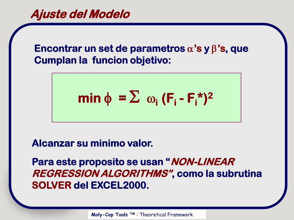
Ajuste del ModeloAjuste del Modelo
Alcanzar su minimo valor.
Para este proposito se usan “NON-LINEAR REGRESSION ALGORITHMS”, como la subrutina
SOLVER del EXCEL2000.
min =wi (Fi - Fi*)2
Encontrar un set de parametros ‟s y b‟s, que
Cumplan la funcion objetivo:
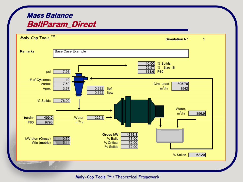
Mass BalanceMass Balance
BallParam_DirectBallParam_Direct
Moly-Cop Tools TM : Theoretical Framework
Moly-Cop Tools TMSimulation N° 1
Remarks
40.00 % Solids
59.97 % - Size 18
psi 7.98 151.0 P80
# of Cyclones 10
Vortex 7.50 Circ. Load 305.79
Apex 3.67 0.382 Bpf m3/hr 1542
0.392 Bpw
% Solids 76.00
Water,
m3/hr 356.9
ton/hr 400.0 Water, 222.1
F80 9795 m3/hr
Gross kW 4316.1
kWh/ton (Gross) 10.79 % Balls 38.00
Wio (metric) 15.14 % Critical 72.00
% Solids 72.00
% Solids 62.20
Base Case Example
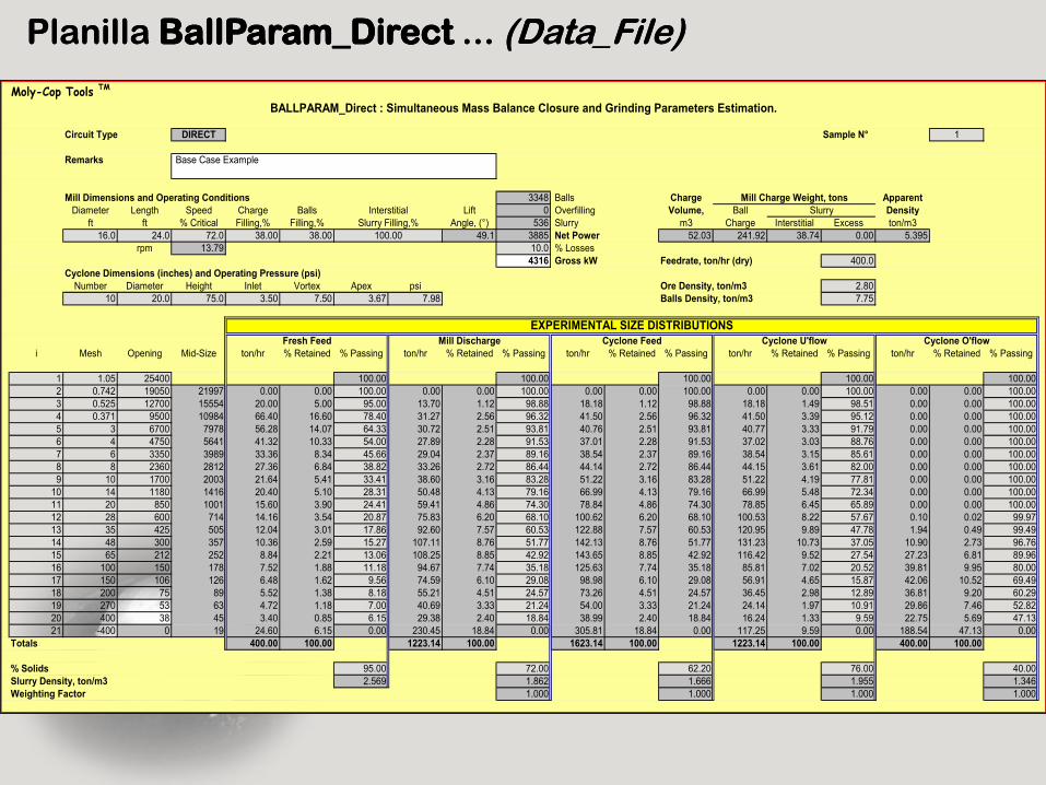
Planilla Planilla BallParam_DirectBallParam_Direct ... ... (Data_File)(Data_File)
Moly-Cop Tools TM
Circuit Type DIRECT Sample N° 1
Remarks
Mill Dimensions and Operating Conditions 3348 Balls Charge Apparent
Diameter Length Speed Charge Balls Lift 0 Overfilling Volume, Ball Density
ft ft % Critical Filling,% Filling,% Angle, (°) 536 Slurry m3 Charge Interstitial Excess ton/m3
16.0 24.0 72.0 38.00 38.00 49.1 3885 Net Power 52.03 241.92 38.74 0.00 5.395
rpm 13.79 10.0 % Losses
4316 Gross kW Feedrate, ton/hr (dry) 400.0
Cyclone Dimensions (inches) and Operating Pressure (psi)
Number Diameter Height Inlet Vortex Apex psi Ore Density, ton/m3 2.80
10 20.0 75.0 3.50 7.50 3.67 7.98 Balls Density, ton/m3 7.75
i Mesh Opening Mid-Size ton/hr % Retained % Passing ton/hr % Retained % Passing ton/hr % Retained % Passing ton/hr % Retained % Passing ton/hr % Retained % Passing
1 1.05 25400 100.00 100.00 100.00 100.00 100.00
2 0.742 19050 21997 0.00 0.00 100.00 0.00 0.00 100.00 0.00 0.00 100.00 0.00 0.00 100.00 0.00 0.00 100.00
3 0.525 12700 15554 20.00 5.00 95.00 13.70 1.12 98.88 18.18 1.12 98.88 18.18 1.49 98.51 0.00 0.00 100.00
4 0.371 9500 10984 66.40 16.60 78.40 31.27 2.56 96.32 41.50 2.56 96.32 41.50 3.39 95.12 0.00 0.00 100.00
5 3 6700 7978 56.28 14.07 64.33 30.72 2.51 93.81 40.76 2.51 93.81 40.77 3.33 91.79 0.00 0.00 100.00
6 4 4750 5641 41.32 10.33 54.00 27.89 2.28 91.53 37.01 2.28 91.53 37.02 3.03 88.76 0.00 0.00 100.00
7 6 3350 3989 33.36 8.34 45.66 29.04 2.37 89.16 38.54 2.37 89.16 38.54 3.15 85.61 0.00 0.00 100.00
8 8 2360 2812 27.36 6.84 38.82 33.26 2.72 86.44 44.14 2.72 86.44 44.15 3.61 82.00 0.00 0.00 100.00
9 10 1700 2003 21.64 5.41 33.41 38.60 3.16 83.28 51.22 3.16 83.28 51.22 4.19 77.81 0.00 0.00 100.00
10 14 1180 1416 20.40 5.10 28.31 50.48 4.13 79.16 66.99 4.13 79.16 66.99 5.48 72.34 0.00 0.00 100.00
11 20 850 1001 15.60 3.90 24.41 59.41 4.86 74.30 78.84 4.86 74.30 78.85 6.45 65.89 0.00 0.00 100.00
12 28 600 714 14.16 3.54 20.87 75.83 6.20 68.10 100.62 6.20 68.10 100.53 8.22 57.67 0.10 0.02 99.97
13 35 425 505 12.04 3.01 17.86 92.60 7.57 60.53 122.88 7.57 60.53 120.95 9.89 47.78 1.94 0.49 99.49
14 48 300 357 10.36 2.59 15.27 107.11 8.76 51.77 142.13 8.76 51.77 131.23 10.73 37.05 10.90 2.73 96.76
15 65 212 252 8.84 2.21 13.06 108.25 8.85 42.92 143.65 8.85 42.92 116.42 9.52 27.54 27.23 6.81 89.96
16 100 150 178 7.52 1.88 11.18 94.67 7.74 35.18 125.63 7.74 35.18 85.81 7.02 20.52 39.81 9.95 80.00
17 150 106 126 6.48 1.62 9.56 74.59 6.10 29.08 98.98 6.10 29.08 56.91 4.65 15.87 42.06 10.52 69.49
18 200 75 89 5.52 1.38 8.18 55.21 4.51 24.57 73.26 4.51 24.57 36.45 2.98 12.89 36.81 9.20 60.29
19 270 53 63 4.72 1.18 7.00 40.69 3.33 21.24 54.00 3.33 21.24 24.14 1.97 10.91 29.86 7.46 52.82
20 400 38 45 3.40 0.85 6.15 29.38 2.40 18.84 38.99 2.40 18.84 16.24 1.33 9.59 22.75 5.69 47.13
21 -400 0 19 24.60 6.15 0.00 230.45 18.84 0.00 305.81 18.84 0.00 117.25 9.59 0.00 188.54 47.13 0.00
Totals 400.00 100.00 1223.14 100.00 1623.14 100.00 1223.14 100.00 400.00 100.00
% Solids 95.00 72.00 62.20 76.00 40.00
Slurry Density, ton/m3 2.569 1.862 1.666 1.955 1.346
Weighting Factor 1.000 1.000 1.000 1.000
Fresh Feed Mill Discharge Cyclone U'flow Cyclone O'flowCyclone Feed
BALLPARAM_Direct : Simultaneous Mass Balance Closure and Grinding Parameters Estimation.
EXPERIMENTAL SIZE DISTRIBUTIONS
Base Case Example
Mill Charge Weight, tons
SlurryInterstitial
Slurry Filling,%
100.00
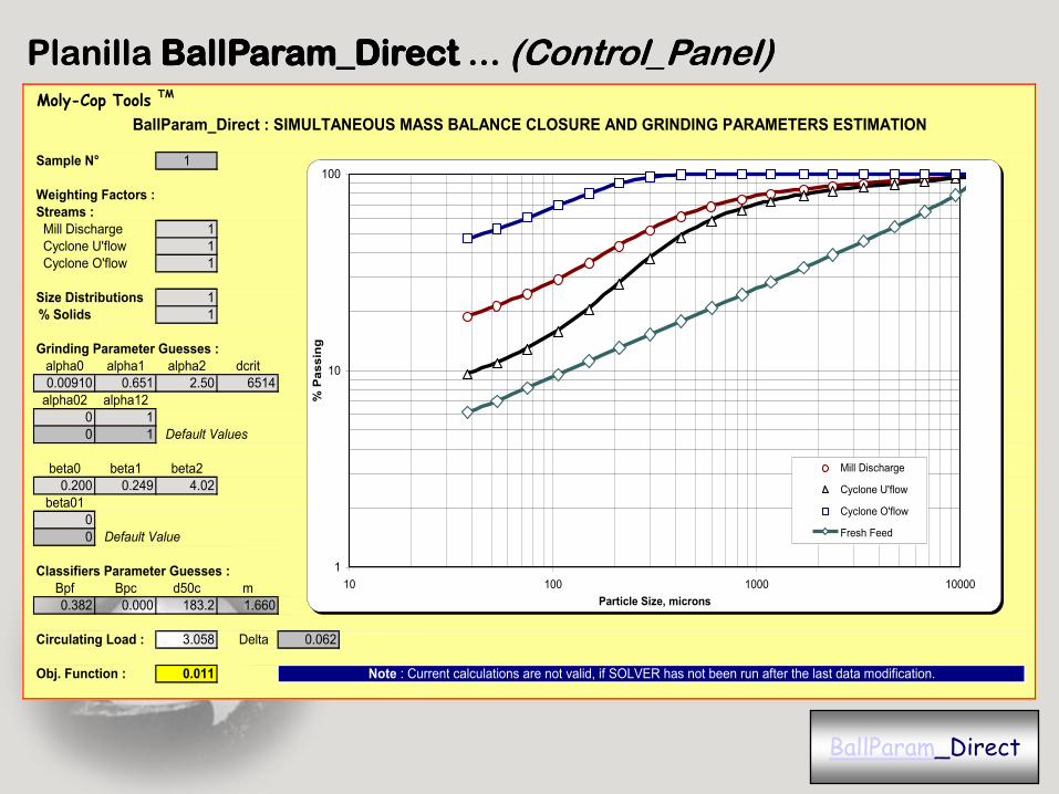
Planilla Planilla BallParam_DirectBallParam_Direct ... ... (Control_Panel)(Control_Panel)
BallParam_Direct
Moly-Cop Tools TM
Sample N° 1
Weighting Factors :
Streams :
Mill Discharge 1
Cyclone U'flow 1
Cyclone O'flow 1
Size Distributions 1
% Solids 1
Grinding Parameter Guesses :
alpha0 alpha1 alpha2 dcrit
0.00910 0.651 2.50 6514 4
alpha02 alpha12
0 1
0 1 Default Values
beta0 beta1 beta2
0.200 0.249 4.02
beta01
0
0 Default Value
Classifiers Parameter Guesses :
Bpf Bpc d50c m
0.382 0.000 183.2 1.660
Circulating Load : 3.058 Delta 0.062
Obj. Function : 0.011 Note : Current calculations are not valid, if SOLVER has not been run after the last data modification.
BallParam_Direct : SIMULTANEOUS MASS BALANCE CLOSURE AND GRINDING PARAMETERS ESTIMATION
1
10
100
10 100 1000 10000
Particle Size, microns
% P
as
sin
g
Mill Discharge
Cyclone U'flow
Cyclone O'flow
Fresh Feed
PlanillaPlanilla
BallParam_DirectBallParam_Direct
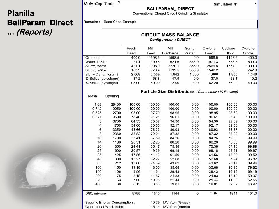
... ... (Reports)(Reports)
Moly-Cop Tools TMSimulation N° 1
Remarks : Base Case Example
Fresh Mill Mill Sump Cyclone Cyclone Cyclone
Feed Feed Discharge Water Feed U'flow O'flow
Ore, ton/hr 400.0 1598.5 1598.5 0.0 1598.5 1198.5 400.0
Water, m3/hr 21.1 399.6 621.6 356.9 971.3 378.5 600.0
Slurry, ton/hr 421.1 1998.0 2220.1 356.9 2569.8 1577.0 1000.0
Slurry, m3/hr 163.9 970.4 1192.5 356.9 1542.2 806.5 742.9
Slurry Dens., ton/m3 2.569 2.059 1.862 1.000 1.666 1.955 1.346
% Solids (by volume) 87.2 58.8 47.9 0.0 37.0 53.1 19.2
% Solids (by weight) 95.00 80.00 72.00 0.00 62.20 76.00 40.00
Mesh Opening
1.05 25400 100.00 100.00 100.00 0.00 100.00 100.00 100.00
0.742 19050 100.00 100.00 100.00 0.00 100.00 100.00 100.00
0.525 12700 95.00 97.70 98.95 0.00 98.95 98.60 100.00
0.371 9500 78.40 91.21 96.61 0.00 96.61 95.48 100.00
3 6700 64.33 85.37 94.30 0.00 94.30 92.39 100.00
4 4750 54.00 80.66 92.17 0.00 92.17 89.56 100.00
6 3350 45.66 76.33 89.93 0.00 89.93 86.57 100.00
8 2360 38.82 72.01 87.32 0.00 87.32 83.09 100.00
10 1700 33.41 67.59 84.26 0.00 84.26 79.00 99.99
14 1180 28.31 62.26 80.20 0.00 80.20 73.60 99.99
20 850 24.41 56.47 75.38 0.00 75.38 67.16 99.99
28 600 20.87 49.39 69.18 0.00 69.18 58.91 99.97
35 425 17.86 41.13 61.56 0.00 61.56 48.90 99.52
48 300 15.27 32.27 52.68 0.00 52.68 37.94 96.82
65 212 13.06 24.39 43.62 0.00 43.62 28.17 89.94
100 150 11.18 18.50 35.68 0.00 35.68 20.95 79.82
150 106 9.56 14.51 29.43 0.00 29.43 16.16 69.19
200 75 8.18 11.87 24.83 0.00 24.83 13.10 59.97
270 53 7.00 10.05 21.44 0.00 21.44 11.06 52.55
400 38 6.15 8.80 19.01 0.00 19.01 9.69 46.92
D80, microns 9795 4510 1164 0 1164 1844 151.0
Specific Energy Consumption : 10.79 kWh/ton (Gross)
Operational Work Index : 15.14 kWh/ton (metric)
BALLPARAM_ DIRECTConventional Closed Circuit Grinding Simulator
CIRCUIT MASS BALANCEConfiguration : DIRECT
Particle Size Distributions (Cummulative % Passing)
PlanillaPlanilla
BallParam_DirectBallParam_Direct
... ... (Reports)(Reports)
Moly-Cop Tools TMSimulation N° 1
Remarks : Base Case Example
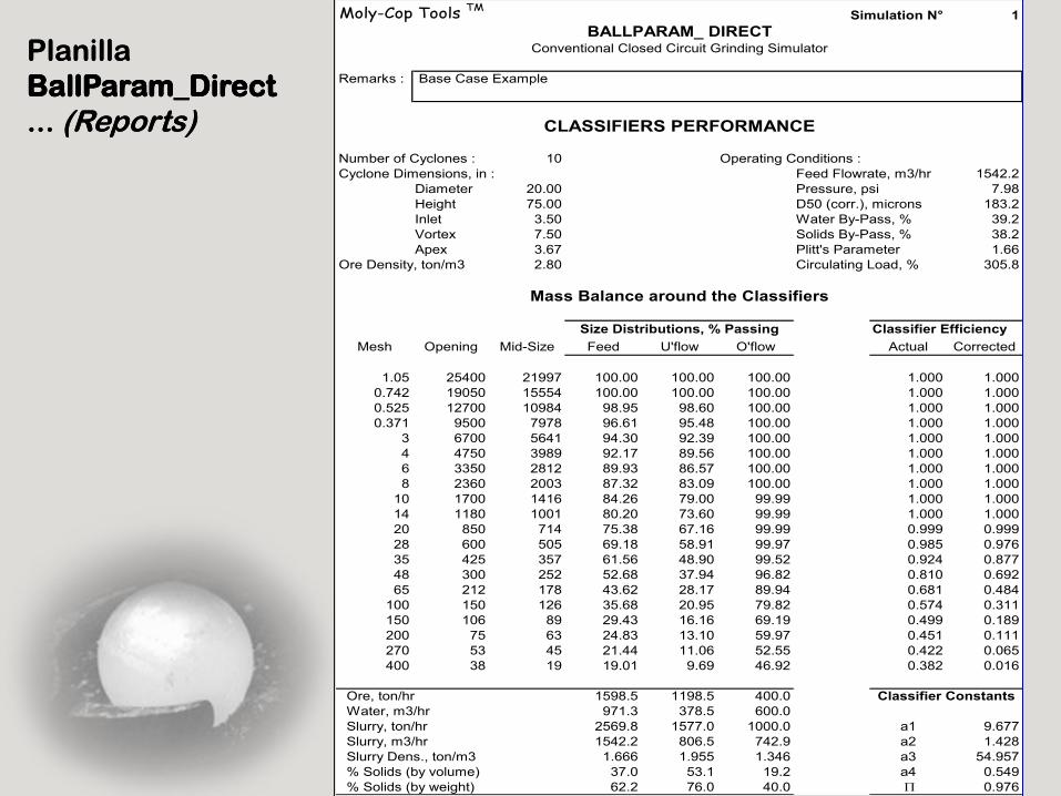
Number of Cyclones : 10 Operating Conditions :
Cyclone Dimensions, in : Feed Flowrate, m3/hr 1542.2
Diameter 20.00 Pressure, psi 7.98
Height 75.00 D50 (corr.), microns 183.2
Inlet 3.50 Water By-Pass, % 39.2
Vortex 7.50 Solids By-Pass, % 38.2
Apex 3.67 Plitt's Parameter 1.66
Ore Density, ton/m3 2.80 Circulating Load, % 305.8
Mesh Opening Mid-Size Feed U'flow O'flow Actual Corrected
1.05 25400 21997 100.00 100.00 100.00 1.000 1.000
0.742 19050 15554 100.00 100.00 100.00 1.000 1.000
0.525 12700 10984 98.95 98.60 100.00 1.000 1.000
0.371 9500 7978 96.61 95.48 100.00 1.000 1.000
3 6700 5641 94.30 92.39 100.00 1.000 1.000
4 4750 3989 92.17 89.56 100.00 1.000 1.000
6 3350 2812 89.93 86.57 100.00 1.000 1.000
8 2360 2003 87.32 83.09 100.00 1.000 1.000
10 1700 1416 84.26 79.00 99.99 1.000 1.000
14 1180 1001 80.20 73.60 99.99 1.000 1.000
20 850 714 75.38 67.16 99.99 0.999 0.999
28 600 505 69.18 58.91 99.97 0.985 0.976
35 425 357 61.56 48.90 99.52 0.924 0.877
48 300 252 52.68 37.94 96.82 0.810 0.692
65 212 178 43.62 28.17 89.94 0.681 0.484
100 150 126 35.68 20.95 79.82 0.574 0.311
150 106 89 29.43 16.16 69.19 0.499 0.189
200 75 63 24.83 13.10 59.97 0.451 0.111
270 53 45 21.44 11.06 52.55 0.422 0.065
400 38 19 19.01 9.69 46.92 0.382 0.016
Ore, ton/hr 1598.5 1198.5 400.0
Water, m3/hr 971.3 378.5 600.0
Slurry, ton/hr 2569.8 1577.0 1000.0 a1 9.677
Slurry, m3/hr 1542.2 806.5 742.9 a2 1.428
Slurry Dens., ton/m3 1.666 1.955 1.346 a3 54.957
% Solids (by volume) 37.0 53.1 19.2 a4 0.549
% Solids (by weight) 62.2 76.0 40.0 0.976
Size Distributions, % Passing
BALLPARAM_ DIRECTConventional Closed Circuit Grinding Simulator
CLASSIFIERS PERFORMANCE
Mass Balance around the Classifiers
Classifier Constants
Classifier Efficiency
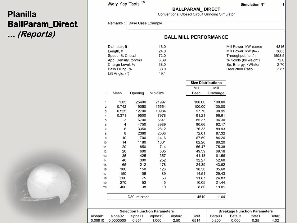
PlanillaPlanilla
BallParam_DirectBallParam_Direct
... ... (Reports)(Reports)
Moly-Cop Tools TMSimulation N° 1
Remarks : Base Case Example
Diameter, ft 16.0 Mill Power, kW (Gross) 4316
Length, ft 24.0 Mill Power, kW (Net) 3885
Speed, % Critical 72.0 Throughput, ton/hr 1598.5
App. Density, ton/m3 5.39 % Solids (by weight) 72.0
Charge Level, % 38.0 Sp. Energy, kWh/ton 2.70
Balls Filling, % 38.0 Reduction Ratio 3.87
Lift Angle, (°) 49.1
Mill Mill
i Mesh Opening Mid-Size Feed Discharge
1 1.05 25400 21997 100.00 100.00
2 0.742 19050 15554 100.00 100.00
3 0.525 12700 10984 97.70 98.95
4 0.371 9500 7978 91.21 96.61
5 3 6700 5641 85.37 94.30
6 4 4750 3989 80.66 92.17
7 6 3350 2812 76.33 89.93
8 8 2360 2003 72.01 87.32
9 10 1700 1416 67.59 84.26
10 14 1180 1001 62.26 80.20
11 20 850 714 56.47 75.38
12 28 600 505 49.39 69.18
13 35 425 357 41.13 61.56
14 48 300 252 32.27 52.68
15 65 212 178 24.39 43.62
16 100 150 126 18.50 35.68
17 150 106 89 14.51 29.43
18 200 75 63 11.87 24.83
19 270 53 45 10.05 21.44
20 400 38 19 8.80 19.01
D80, microns 4510 1164
alpha01 alpha02 alpha11 alpha12 alpha2 Dcrit Beta00 Beta01 Beta1 Beta2
0.00910 0.0000000 0.651 1.000 2.50 6514 0.200 0.000 0.25 4.02
Breakage Function ParametersSelection Function Parameters
Size Distributions
BALL MILL PERFORMANCE
BALLPARAM_ DIRECTConventional Closed Circuit Grinding Simulator
Theoretical FrameworkTheoretical Framework
SIMULACION DE CIRCUITOS DE SIMULACION DE CIRCUITOS DE
MOLIENDA / CLASIFICACIONMOLIENDA / CLASIFICACION
Se
ttin
g N
ew
Sta
nd
ard
Me
tho
do
log
ies
in
Se
ttin
g N
ew
Sta
nd
ard
Me
tho
do
log
ies
in
Gri
nd
ing
Pro
ce
ss
An
aly
sis
Gri
nd
ing
Pro
ce
ss
An
aly
sis
Developed by Moly-Cop Grinding Systems
Moly-Cop Tools TM : Theoretical Framework
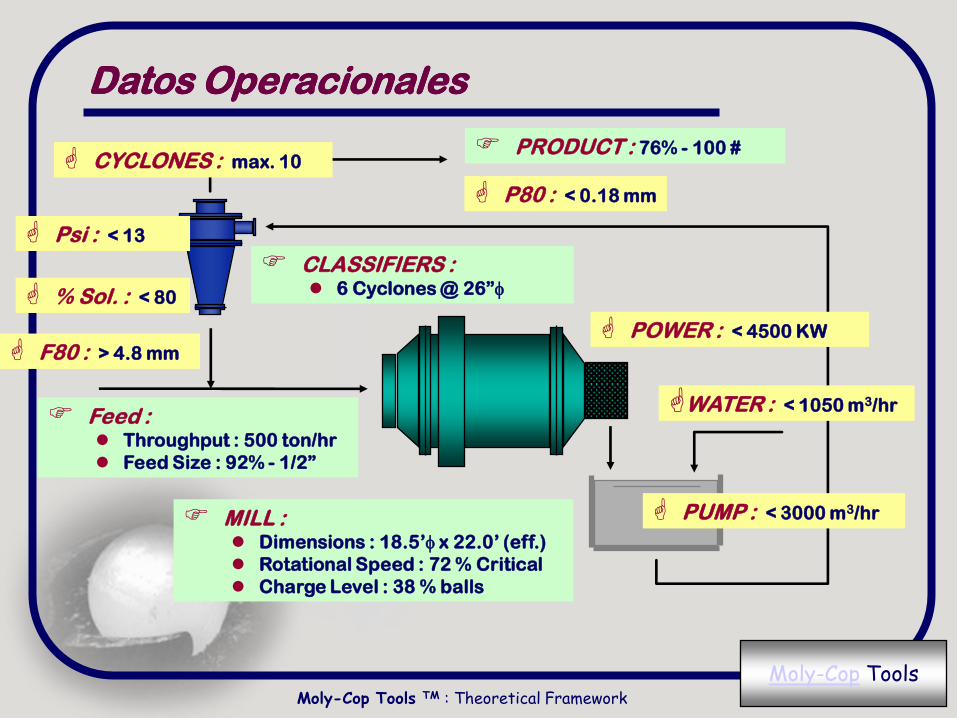
MILL : Dimensions : 18.5‟ x 22.0‟ (eff.)
Rotational Speed : 72 % Critical
Charge Level : 38 % balls
MILL : Dimensions : 18.5‟ x 22.0‟ (eff.)
Rotational Speed : 72 % Critical
Charge Level : 38 % balls
CLASSIFIERS : 6 Cyclones @ 26”
CLASSIFIERS : 6 Cyclones @ 26”
Feed : Throughput : 500 ton/hr
Feed Size : 92% - 1/2”
Feed : Throughput : 500 ton/hr
Feed Size : 92% - 1/2”
PRODUCT : 76% - 100 # PRODUCT : 76% - 100 #
Datos OperacionalesDatos Operacionales
POWER : < 4500 KW POWER : < 4500 KW
CYCLONES : max. 10 CYCLONES : max. 10
F80 : > 4.8 mm F80 : > 4.8 mm
P80 : < 0.18 mm P80 : < 0.18 mm
WATER : < 1050 m3/hrWATER : < 1050 m3/hr
PUMP : < 3000 m3/hr PUMP : < 3000 m3/hr
% Sol. : < 80 % Sol. : < 80
Psi : < 13 Psi : < 13
Moly-Cop Tools

Planilla Planilla BallSim_DirectBallSim_Direct ... ... (Data_File)(Data_File)
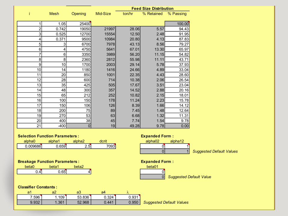
i Mesh Opening Mid-Size ton/hr % Retained % Passing
1 1.05 25400 100.00
2 0.742 19050 21997 28.06 5.57 94.43
3 0.525 12700 15554 12.50 2.48 91.95
4 0.371 9500 10984 20.80 4.13 87.83
5 3 6700 7978 43.13 8.56 79.27
6 4 4750 5641 67.01 13.30 65.97
7 6 3350 3989 56.20 11.15 54.82
8 8 2360 2812 55.98 11.11 43.71
9 10 1700 2003 29.14 5.78 37.93
10 14 1180 1416 24.66 4.89 33.04
11 20 850 1001 22.35 4.43 28.60
12 28 600 714 10.38 2.06 26.54
13 35 425 505 17.67 3.51 23.04
14 48 300 357 14.52 2.88 20.16
15 65 212 252 10.82 2.15 18.01
16 100 150 178 11.24 2.23 15.78
17 150 106 126 8.39 1.66 14.12
18 200 75 89 7.45 1.48 12.64
19 270 53 63 6.68 1.32 11.31
20 400 38 45 7.74 1.54 9.78
21 -400 0 19 49.28 9.78 0.00
Selection Function Parameters : Expanded Form :
alpha0 alpha1 alpha2 dcrit alpha02 alpha12
0.009686 0.659 2.5 7093 0 1
0 1 Suggested Default Values
Breakage Function Parameters : Expanded Form :
beta0 beta1 beta2 beta01
0.4 0.65 4 0
0 Suggested Default Value
Classifier Constants :
a1 a2 a3 a4
7.596 1.109 53.836 0.324 0.931
9.932 1.361 52.968 0.441 0.950 Suggested Default Values
Feed Size Distribution

Planilla Planilla BallSim_DirectBallSim_Direct ... ... (Data_File)(Data_File)
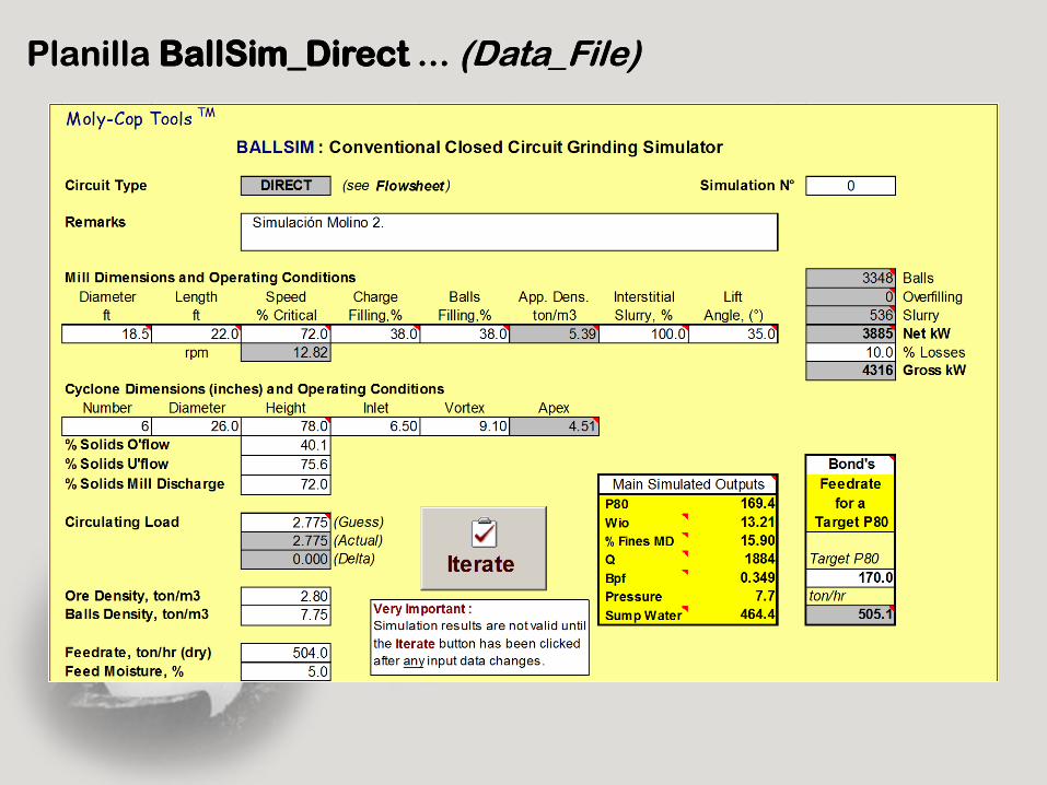
Planilla Planilla BallSim_DirectBallSim_Direct ... ... (Data_File)(Data_File)
PlanillaPlanilla
BallSim_DirectBallSim_Direct
... ... (Reports)(Reports)
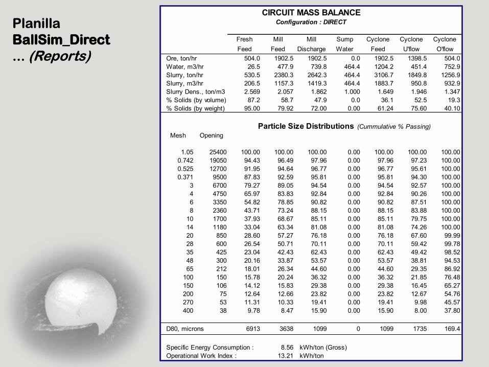
Fresh Mill Mill Sump Cyclone Cyclone Cyclone
Feed Feed Discharge Water Feed U'flow O'flow
Ore, ton/hr 504.0 1902.5 1902.5 0.0 1902.5 1398.5 504.0
Water, m3/hr 26.5 477.9 739.8 464.4 1204.2 451.4 752.9
Slurry, ton/hr 530.5 2380.3 2642.3 464.4 3106.7 1849.8 1256.9
Slurry, m3/hr 206.5 1157.3 1419.3 464.4 1883.7 950.8 932.9
Slurry Dens., ton/m3 2.569 2.057 1.862 1.000 1.649 1.946 1.347
% Solids (by volume) 87.2 58.7 47.9 0.0 36.1 52.5 19.3
% Solids (by weight) 95.00 79.92 72.00 0.00 61.24 75.60 40.10
Mesh Opening
1.05 25400 100.00 100.00 100.00 0.00 100.00 100.00 100.00
0.742 19050 94.43 96.49 97.96 0.00 97.96 97.23 100.00
0.525 12700 91.95 94.64 96.77 0.00 96.77 95.61 100.00
0.371 9500 87.83 92.59 95.81 0.00 95.81 94.30 100.00
3 6700 79.27 89.05 94.54 0.00 94.54 92.57 100.00
4 4750 65.97 83.83 92.84 0.00 92.84 90.26 100.00
6 3350 54.82 78.85 90.82 0.00 90.82 87.51 100.00
8 2360 43.71 73.24 88.15 0.00 88.15 83.88 100.00
10 1700 37.93 68.67 85.11 0.00 85.11 79.75 100.00
14 1180 33.04 63.34 81.08 0.00 81.08 74.26 100.00
20 850 28.60 57.27 76.18 0.00 76.18 67.60 99.99
28 600 26.54 50.71 70.11 0.00 70.11 59.42 99.78
35 425 23.04 42.43 62.43 0.00 62.43 49.42 98.52
48 300 20.16 33.87 53.57 0.00 53.57 38.81 94.53
65 212 18.01 26.34 44.60 0.00 44.60 29.35 86.92
100 150 15.78 20.24 36.32 0.00 36.32 21.85 76.48
150 106 14.12 15.83 29.38 0.00 29.38 16.45 65.27
200 75 12.64 12.66 23.82 0.00 23.82 12.67 54.76
270 53 11.31 10.33 19.41 0.00 19.41 9.98 45.57
400 38 9.78 8.47 15.90 0.00 15.90 8.00 37.80
D80, microns 6913 3638 1099 0 1099 1735 169.4
Specific Energy Consumption : 8.56 kWh/ton (Gross)
Operational Work Index : 13.21 kWh/ton
CIRCUIT MASS BALANCEConfiguration : DIRECT
Particle Size Distributions (Cummulative % Passing)

PlanillaPlanilla
BallSim_DirectBallSim_Direct
... ... (Reports)(Reports)
Number of Cyclones : 6 Operating Conditions :
Cyclone Dimensions, in : Feed Flowrate, m3/hr 1883.7
Diameter 26.00 Pressure, psi 7.7
Height 78.00 D50 (corr.), microns 183.3
Inlet 6.50 Water By-Pass, % 37.5
Vortex 9.10 Solids By-Pass, % 34.9
Apex 4.51 Plitt's Parameter 1.34
Ore Density, ton/m3 2.80 Circulating Load, % 277
Mesh Opening Mid-Size Feed U'flow O'flow Actual Corrected
1.05 25400 21997 100.00 100.00 100.00 1.000 1.000
0.742 19050 15554 97.96 97.23 100.00 1.000 1.000
0.525 12700 10984 96.77 95.61 100.00 1.000 1.000
0.371 9500 7978 95.81 94.30 100.00 1.000 1.000
3 6700 5641 94.54 92.57 100.00 1.000 1.000
4 4750 3989 92.84 90.26 100.00 1.000 1.000
6 3350 2812 90.82 87.51 100.00 1.000 1.000
8 2360 2003 88.15 83.88 100.00 1.000 1.000
10 1700 1416 85.11 79.75 100.00 1.000 1.000
14 1180 1001 81.08 74.26 100.00 0.999 0.999
20 850 714 76.18 67.60 99.99 0.991 0.986
28 600 505 70.11 59.42 99.78 0.956 0.933
35 425 357 62.43 49.42 98.52 0.881 0.817
48 300 252 53.57 38.81 94.53 0.775 0.655
65 212 178 44.60 29.35 86.92 0.666 0.487
100 150 126 36.32 21.85 76.48 0.572 0.342
150 106 89 29.38 16.45 65.27 0.500 0.231
200 75 63 23.82 12.67 54.76 0.448 0.152
270 53 45 19.41 9.98 45.57 0.414 0.099
400 38 19 15.90 8.00 37.80 0.370 0.032
Ore, ton/hr 1902.5 1398.5 504.0
Water, m3/hr 1204.2 451.4 752.9
Slurry, ton/hr 3106.7 1849.8 1256.9 a1 7.596
Slurry, m3/hr 1883.7 950.8 932.9 a2 1.109
Slurry Dens., ton/m3 1.649 1.946 1.347 a3 53.836
% Solids (by volume) 36.1 52.5 19.3 a4 0.324
% Solids (by weight) 61.2 75.6 40.1 0.931
CLASSIFIERS PERFORMANCE
Mass Balance around the Classifiers
Classifier Constants
Classifier EfficiencySize Distributions, % Passing
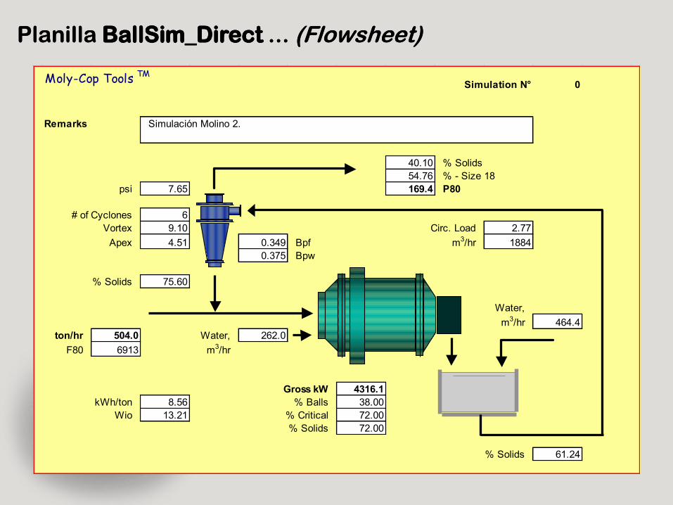
Planilla Planilla BallSim_DirectBallSim_Direct ... ... (Flowsheet)(Flowsheet)
Moly-Cop Tools TMSimulation N° 0
Remarks
40.10 % Solids
54.76 % - Size 18
psi 7.65 169.4 P80
# of Cyclones 6
Vortex 9.10 Circ. Load 2.77
Apex 4.51 0.349 Bpf m3/hr 1884
0.375 Bpw
% Solids 75.60
Water,
m3/hr 464.4
ton/hr 504.0 Water, 262.0
F80 6913 m3/hr
Gross kW 4316.1
kWh/ton 8.56 % Balls 38.00
Wio 13.21 % Critical 72.00
% Solids 72.00
% Solids 61.24
Simulación Molino 2.
Se
ttin
g N
ew
Sta
nd
ard
Me
tho
do
log
ies
in
Se
ttin
g N
ew
Sta
nd
ard
Me
tho
do
log
ies
in
Gri
nd
ing
Pro
ce
ss
An
aly
sis
Gri
nd
ing
Pro
ce
ss
An
aly
sis
Process OptimizationProcess Optimization
DETERMINACION DEL TAMAÑO DETERMINACION DEL TAMAÑO
OPTIMO DE MEDIOS DE MOLIENDAOPTIMO DE MEDIOS DE MOLIENDA
Developed by Moly-Cop Grinding Systems
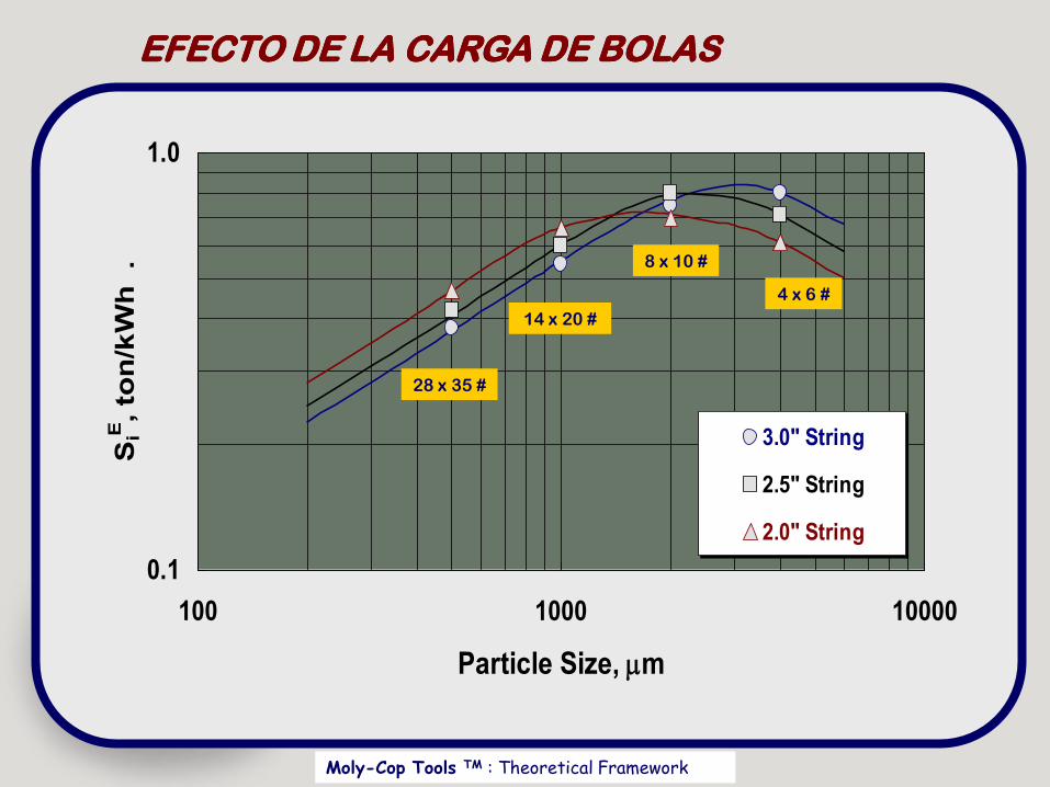
Moly-Cop Tools TM : Theoretical Framework
0.1
1.0
100 1000 10000
Particle Size, mm
SiE
, to
n/k
Wh
.
3.0" String
2.5" String
2.0" String
EFECTO DE LA CARGA DE BOLASEFECTO DE LA CARGA DE BOLAS
28 x 35 #
14 x 20 #
8 x 10 #
4 x 6 #
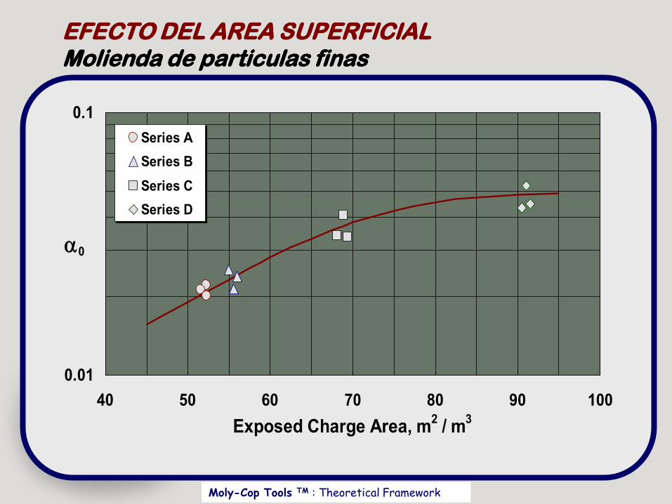
Moly-Cop Tools TM : Theoretical Framework
0.01
0.1
40 50 60 70 80 90 100
Exposed Charge Area, m2 / m
3
0
Series A
Series B
Series C
Series D
EFECTO DEL AREA SUPERFICIALEFECTO DEL AREA SUPERFICIALMolienda de particulas finasMolienda de particulas finas
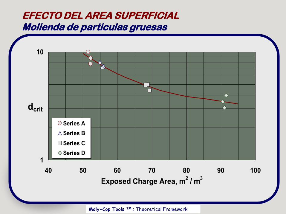
Moly-Cop Tools TM : Theoretical Framework
1
10
40 50 60 70 80 90 100
Exposed Charge Area, m2 / m
3
dcrit
Series A
Series B
Series C
Series D
EFECTO DEL AREA SUPERFICIALEFECTO DEL AREA SUPERFICIALMolienda de particulas gruesasMolienda de particulas gruesas
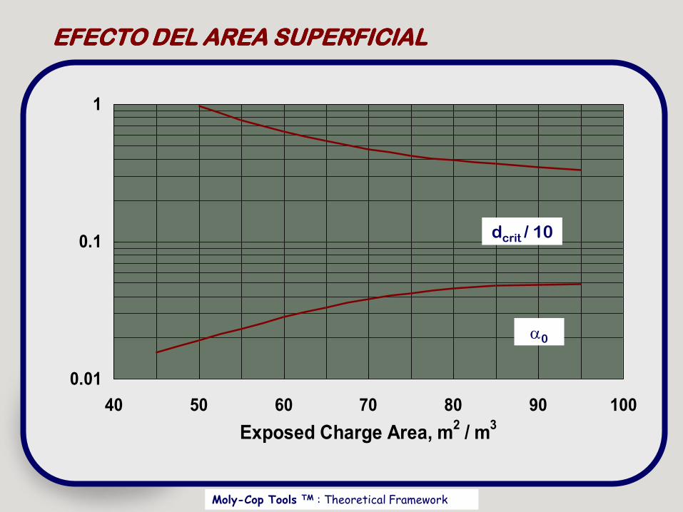
Moly-Cop Tools TM : Theoretical Framework
0.01
0.1
1
40 50 60 70 80 90 100
Exposed Charge Area, m2 / m
3
EFECTO DEL AREA SUPERFICIALEFECTO DEL AREA SUPERFICIAL
dcrit / 10
0
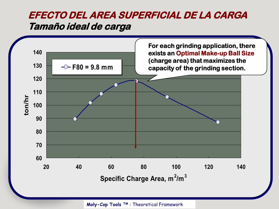
Moly-Cop Tools TM : Theoretical Framework
60
70
80
90
100
110
120
130
140
20 40 60 80 100 120 140
Specific Charge Area, m2/m
3
ton
/hr
F80 = 9.8 mm
For each grinding application, there
exists an Optimal Make-up Ball Size
(charge area) that maximizes the
capacity of the grinding section.
EFECTO DEL AREA SUPERFICIAL DE LA CARGAEFECTO DEL AREA SUPERFICIAL DE LA CARGATamaño ideal de cargaTamaño ideal de carga
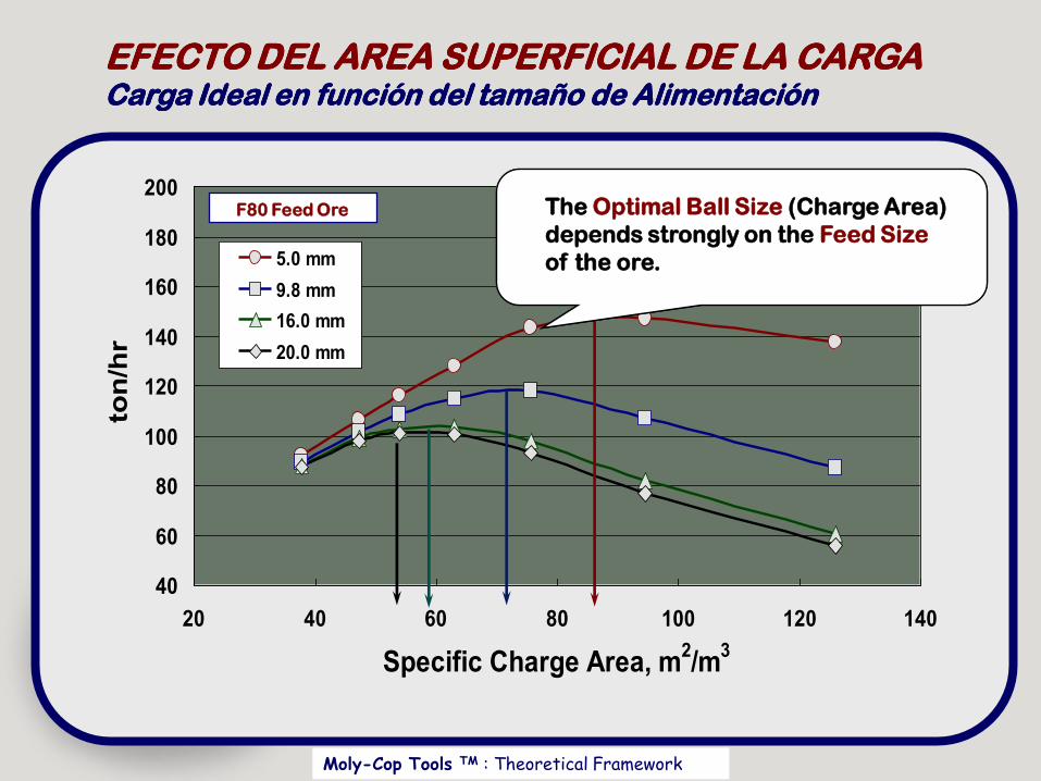
Moly-Cop Tools TM : Theoretical Framework
40
60
80
100
120
140
160
180
200
20 40 60 80 100 120 140
Specific Charge Area, m2/m
3
to
n/h
r
5.0 mm
9.8 mm
16.0 mm
20.0 mm
F80 Feed Ore The Optimal Ball Size (Charge Area)
depends strongly on the Feed Size
of the ore.
EFECTO DEL AREA SUPERFICIAL DE LA CARGAEFECTO DEL AREA SUPERFICIAL DE LA CARGACarga Ideal en función del tamaño de AlimentaciónCarga Ideal en función del tamaño de Alimentación
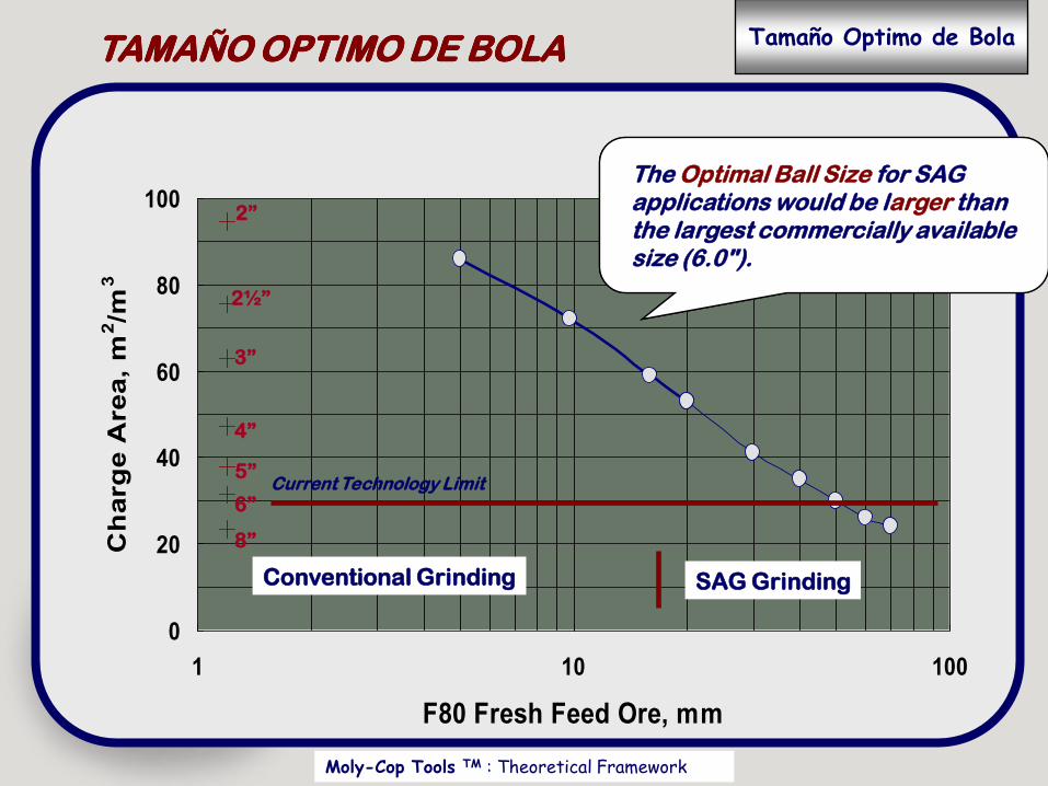
Moly-Cop Tools TM : Theoretical Framework
TAMAÑO OPTIMO DE BOLATAMAÑO OPTIMO DE BOLA
0
20
40
60
80
100
1 10 100
F80 Fresh Feed Ore, mm
Ch
arg
e A
rea,
m2/m
3
Conventional Grinding SAG Grinding
Current Technology Limit
2”
2½”
3”
4”
5”
6”
8”
The Optimal Ball Size for SAGapplications would be larger thanthe largest commercially availablesize (6.0").
Tamaño Optimo de Bola

Podrian imaginar que sienteuna pobre partícula cuando
Es atacada por una bola de 6.0”...?
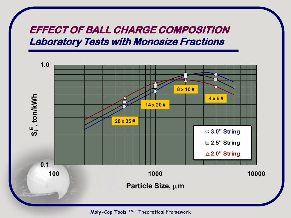
0.1
1.0
100 1000 10000
Particle Size, mm
SiE
, to
n/k
Wh
3.0" String
2.5" String
2.0" String
EFFECT OF BALL CHARGE COMPOSITIONEFFECT OF BALL CHARGE COMPOSITIONLaboratory Tests with Monosize FractionsLaboratory Tests with Monosize Fractions
28 x 35 #
14 x 20 #
8 x 10 #
4 x 6 #
Moly-Cop Tools TM : Theoretical Framework
Moly-Cop Tools TM : Theoretical Framework
Existe una natural creencia de que al recargar una
combinación de bolas de distintos diámetros, se lograríauna mejor eficiencia de la molienda de las partículasgruesas (por la acción de las bolas más grandes) y a lavez, una mejor eficiencia para las partículas finas (por laacción de las bolas más pequeñas).
Sin embargo, así como las bolas de mayor diámetro seríaneficientes para fracturar las partículas más gruesas, almismo tiempo, serían relativamente ineficientes parafracturar las partículas más finas ... mientras lo contrarioaplicaría para las bolas más pequeñas.
El resultado combinado de ambos collares de bolas seríaequivalente al de un collar de recarga única con bolas deun tamaño tal que exponga igual área específica enm2/m3.
DIAMETROS MULTIPLES DE RECARGADIAMETROS MULTIPLES DE RECARGADIAMETROS MULTIPLES DE RECARGADIAMETROS MULTIPLES DE RECARGA
Recarga Multiple
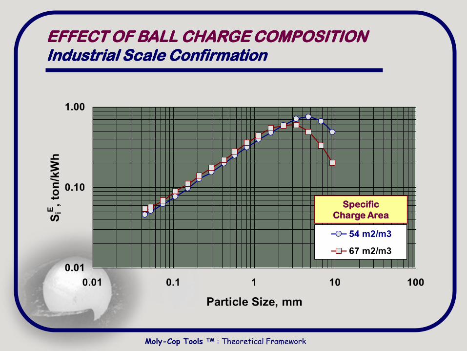
0.01
0.10
1.00
0.01 0.1 1 10 100
Particle Size, mm
SiE
, to
n/k
Wh
54 m2/m3
67 m2/m3
EFFECT OF BALL CHARGE COMPOSITIONEFFECT OF BALL CHARGE COMPOSITIONIndustrial Scale ConfirmationIndustrial Scale Confirmation
Specific
Charge Area
Moly-Cop Tools TM : Theoretical Framework
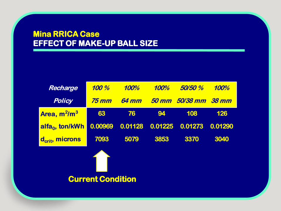
Mina RRICA CaseMina RRICA Case
EFFECT OF MAKEEFFECT OF MAKE--UP BALL SIZEUP BALL SIZE
Recharge 100 % 100% 100% 50/50 % 100%
Policy 75 mm 64 mm 50 mm 50/38 mm 38 mm
Area, m2/m3 63 76 94 108 126
alfa0, ton/kWh 0.00969 0.01128 0.01225 0.01273 0.01290
dcrit, microns 7093 5079 3853 3370 3040
Current ConditionCurrent Condition
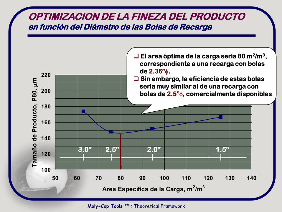
Moly-Cop Tools TM : Theoretical Framework
100
120
140
160
180
200
220
50 60 70 80 90 100 110 120 130 140
Area Específica de la Carga, m2/m
3
Ta
ma
ño
de
Pro
du
cto
, P
80
, m
m
El area óptima de la carga sería 80 m2/m3,
correspondiente a una recarga con bolas
de 2.36”.
Sin embargo, la eficiencia de estas bolas
sería muy similar al de una recarga con
bolas de 2.5”, comercialmente disponibles
OPTIMIZACION DE LA FINEZA DEL PRODUCTOOPTIMIZACION DE LA FINEZA DEL PRODUCTOen función del Diámetro de las Bolas de Recargaen función del Diámetro de las Bolas de Recarga
3.0”3.0” 2.5”2.5” 2.0”2.0” 1.5”1.5”
Se
ttin
g N
ew
Sta
nd
ard
Me
tho
do
log
ies
in
Se
ttin
g N
ew
Sta
nd
ard
Me
tho
do
log
ies
in
Gri
nd
ing
Pro
ce
ss
An
aly
sis
Gri
nd
ing
Pro
ce
ss
An
aly
sis
GRACIASGRACIAS
Developed by Moly-Cop Grinding Systems