Molecular valves for controlling gas phase transport made

1

Molecular Valves for Controlling Gas Phase Transport Made from Discrete Angstrom-Sized Pores in Graphene

Luda Wang1,7, Lee W. Drahushuk2, Lauren Cantley3, Steven P. Koenig4,5, Xinghui Liu1,

John Pellegrino1, Michael S. Strano2, and J. Scott Bunch3,6*

*e-mail: [email protected]

Supplementary Information:

1. Leak rate through the silicon oxide substrate

The leak rate can be derived from the ideal gas law and Hencky’s solution for a clamped circular membrane and follows closely reference1:

2 3 204 4

1 [3 ]b atmdn Et Et dK V V P K C adt RT a a dt

(S1)

where R is the gas constant, T is the temperature, E = 1 TPa is the Young’s modulus, t = 0.335 nm is the thickness of the membrane, a is the radius of the membrane, V0 is the microcavity volume at zero deflection, Vb is the bulged up volume, Patm is the ambient pressure, δ is the maximum deflection of the membrane, K(ν = 0.16) = 3.09, and C(ν = 0.16) = 0.52 are constants determined by the Hencky’s solution.

The maximum deflection versus time was measured for pristine unetched graphene (Supplementary Fig. 1). The samples were inserted into the high pressure chamber with ~300 kPa charging H2. After a few weeks, the internal pressure of the microcavity reached equilibrium with the charging pressure. Continuous AFM scanning was taken during the first 100 min of removal from the pressure chamber, and the deflection decreased by a few nanometres. From the slope of the deflection vs. time and equation S1, we determine that the permeance is ~6 x 10-25mol s-1Pa-1, which is at least one order of magnitude lower than the H2 permeance of the porous graphene.

Molecular valves for controlling gas phase transport made from discrete ångström-sized

pores in graphene

SUPPLEMENTARY INFORMATIONDOI: 10.1038/NNANO.2015.158

NATURE NANOTECHNOLOGY | www.nature.com/naturenanotechnology 1

© 2015 Macmillan Publishers Limited. All rights reserved

http://dx.doi.org/10.1038/nnano.2015.158

2

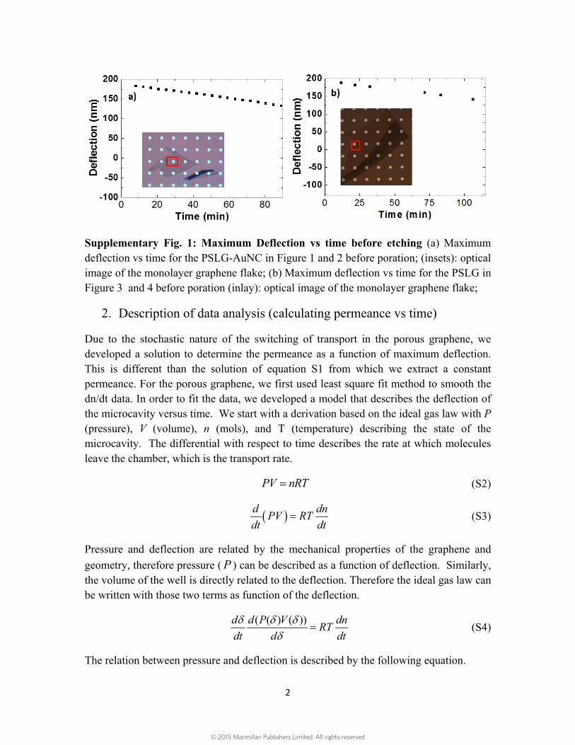
Supplementary Fig. 1: Maximum Deflection vs time before etching (a) Maximum deflection vs time for the PSLG-AuNC in Figure 1 and 2 before poration; (insets): optical image of the monolayer graphene flake; (b) Maximum deflection vs time for the PSLG in Figure 3 and 4 before poration (inlay): optical image of the monolayer graphene flake;

2. Description of data analysis (calculating permeance vs time)

Due to the stochastic nature of the switching of transport in the porous graphene, we developed a solution to determine the permeance as a function of maximum deflection. This is different than the solution of equation S1 from which we extract a constant permeance. For the porous graphene, we first used least square fit method to smooth the dn/dt data. In order to fit the data, we developed a model that describes the deflection of the microcavity versus time. We start with a derivation based on the ideal gas law with P (pressure), V (volume), n (mols), and T (temperature) describing the state of the microcavity. The differential with respect to time describes the rate at which molecules leave the chamber, which is the transport rate.

PV nRT (S2)

d dnPV RT

dt dt (S3)

Pressure and deflection are related by the mechanical properties of the graphene and

geometry, therefore pressure ( P ) can be described as a function of deflection. Similarly, the volume of the well is directly related to the deflection. Therefore the ideal gas law can be written with those two terms as function of the deflection.

( ( ) ( ))d d P V dnRT

dt d dt

(S4)

The relation between pressure and deflection is described by the following equation.


3

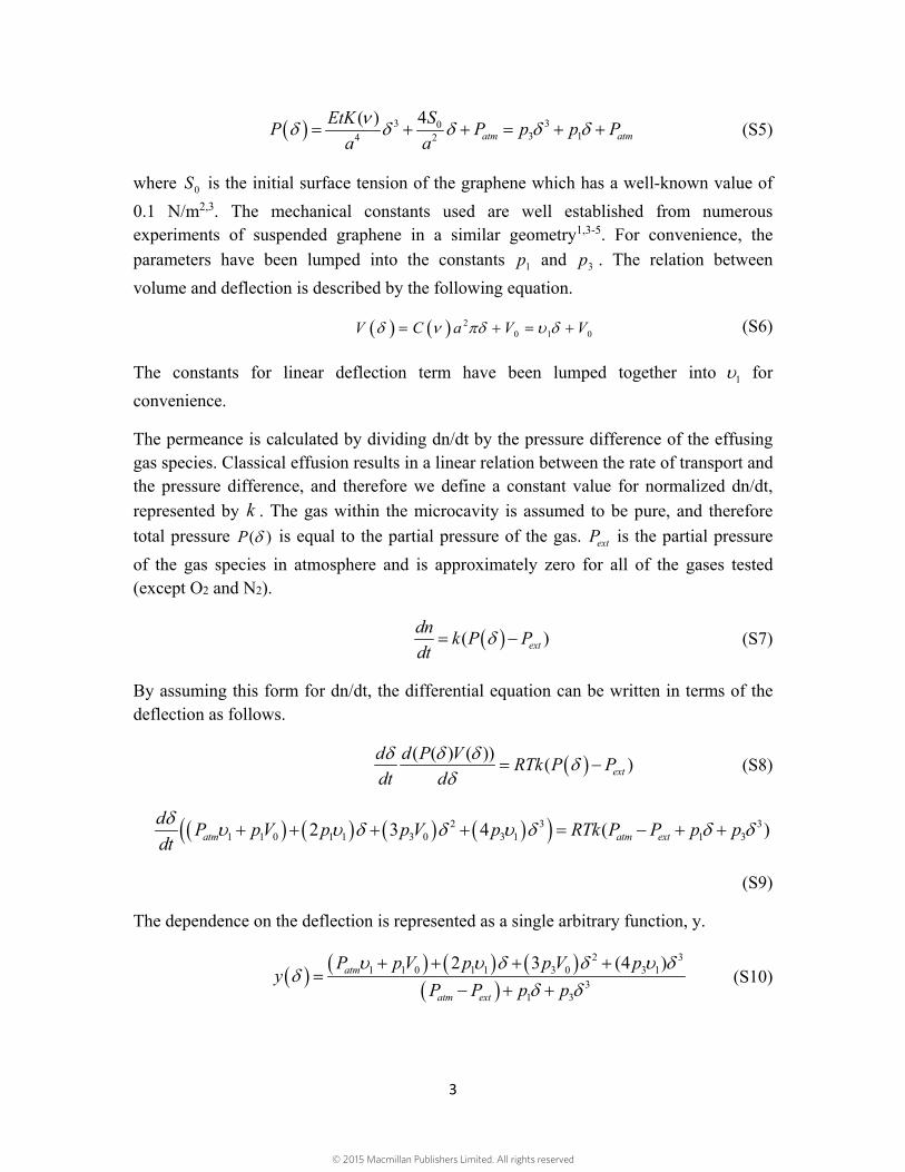
3 303 14 2

4( )atm atm

SEtKP P p p P

a a

(S5)

where 0S is the initial surface tension of the graphene which has a well-known value of

0.1 N/m2,3. The mechanical constants used are well established from numerous experiments of suspended graphene in a similar geometry1,3-5. For convenience, the

parameters have been lumped into the constants 1p and 3p . The relation between

volume and deflection is described by the following equation.

20 1 0V C a V V (S6)

The constants for linear deflection term have been lumped together into 1 for

convenience.

The permeance is calculated by dividing dn/dt by the pressure difference of the effusing gas species. Classical effusion results in a linear relation between the rate of transport and the pressure difference, and therefore we define a constant value for normalized dn/dt,

represented by k . The gas within the microcavity is assumed to be pure, and therefore

total pressure ( )P is equal to the partial pressure of the gas. extP is the partial pressure

of the gas species in atmosphere and is approximately zero for all of the gases tested (except O2 and N2).

( )ext

dnk P P

dt (S7)

By assuming this form for dn/dt, the differential equation can be written in terms of the deflection as follows.

( ( ) ( ))( )ext

d d P VRTk P P

dt d

(S8)

2 3 31 1 0 1 1 3 0 3 1 1 32 3 4 ( )atm atm ext

dP pV p p V p RTk P P p p

dt

(S9)

The dependence on the deflection is represented as a single arbitrary function, y.

2 31 1 0 1 1 3 0 3 1

31 3

2 3 (4 )atm

atm ext

P pV p p V py

P P p p

(S10)


4

dy RTk

dt

(S11)

The differential equation is separable and can be solved.

0 0

ty d RTk dt

(S12)

0Y Y RTkt (S13)

The resulting form is a line. The values of the integral, ( )Y , can be calculated

numerically for each experimental deflection point. A segment of these values is fit using

the analytical least squares line fit, and gives results for 0( )Y and k when temperature

is known.

For the results of permeance or flux in the main paper, the fitting method is applied to a segment of 5 data points, and the resulting values are assigned to the centre data point. A value of k, the permeance, is calculated at each point by proceeding through the data set in this manner. Permeance values in the main text only include points with deflection above 50 nm. Points below 50 nm were excluded because small errors in the pressure correlation, and small amounts of air in the microcavity in some runs results in large errors in the permeance calculation at points lower than 50 nm deflection. When a full five points aren’t available for the points at the beginning and end of the deflection data set, only the three or four nearest points are used to fit a value of permeation.

3. Deflection fitting (Fig.1s)

Figure 1s of the main paper plots an extrapolated fit of the deflection data before the sudden drop in deflection. This extrapolation represents the expected trajectory if the pore had continued in the state (blocked) at the start of the measurement. It was calculated by numerically linearizing the deflection data prior to the sudden drop (0 to 12 min) via S12 to the form of S13. From the analytical least squares fit, values for the two

parameters, 0( )Y and k , can be determined based on all the points in the range of 0 to

12 min.

To create a fit and extrapolation for the deflection, a set of arbitrary, evenly spaced deflection values between the maximum and minimum deflections are put in the form of S13. The fitted values of the two parameters, Y(δ0) and k, are used to solve for time at each of the arbitrary deflection points. Then the arbitrary deflection points are plotted against the calculated times as the fit and extrapolation.

4. Reversible switching of permeance from laser heating


5

Figure 2 of the main text shows switching of the permeance by laser induced heating which moves the AuNCs towards the pore site. This process is reversible. Further experiments on the same PSLG-AuNCs as in Figure 2 continue to show a slow permeance (gray coloured bar). Additional laser induced heating of the graphene resulted in a faster permeance shown by the magenta coloured bars in Supplementary Fig. 2.

Supplementary Fig. 2 Reversible switching of permeance from laser heating Histogram of the permeance from (data in gray) to (data in magenta) by a second laser induced heating event.

5. Comparison to Classical Effusion

Supplementary Fig. 3 is used to compare selectivities predicted by the classical effusion model. Classical effusion requires the pore size to be smaller than the mean free path of the gas molecules which is around 60 nm at room temperature. However, we are in a regime where the angstrom-sized pore is much smaller than the mean free path and comparable to the size of the gas molecules. In this case, the molecular size, geometry, and chemistry should be considered.

In simple classical effusion, the permeance through a pore would be inversely proportional to the square root of the molecular mass (Mw

1/2), and the selectivity is the ratio of the Mw

1/2. This is 1.4, 3.2, 3.7, 4, 4.5, 4.7, 4.7 for H2 to He, Ne, N2, O2, Ar, N2O, CO2, respectively. However, the selectivity from our experiment is dramatically different as predicted from classical effusion (Table 1). This is most clearly seen when comparing O2 and N2. The permeance of O2 is 2.6x the permeance of N2 despite O2 having a larger Mw suggesting that our experiment is not in the classical effusion regime and we must consider the kinetic diameter. O2 has a slightly smaller kinetic diameter compared to N2. Supplementary Fig. 3d which plots the permeance of the Noble gases measured show strong deviations from classical effusion. The permeance of Ar is significantly lower than expected for classical effusion suggesting that molecular sieving is taking place based on the kinetic diameter.


6

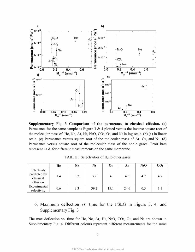
Supplementary Fig. 3 Comparison of the permeance to classical effusion. (a) Permeance for the same sample as Figure 3 & 4 plotted versus the inverse square root of the molecular mass of He, Ne, Ar, H2, N2O, CO2, O2, and N2 in log scale. (b) (a) in linear scale. (c) Permeance versus square root of the molecular mass of Ar, O2, and N2. (d) Permeance versus square root of the molecular mass of the noble gases. Error bars represent ±s.d. for different measurements on the same membrane.

TABLE 1 Selectivities of H2 to other gases

He Ne N2 O2 Ar N2O CO2 Selectivity

predicted by classical effusion

1.4 3.2 3.7 4 4.5 4.7 4.7

Experimental selectivity

0.6 3.3 39.2 15.1 24.6 0.5 1.1

6. Maximum deflection vs. time for the PSLG in Figure 3, 4, and Supplementary Fig. 3

The max deflection vs. time for He, Ne, Ar, H2, N2O, CO2, O2, and N2 are shown in Supplementary Fig. 4. Different colours represent different measurements for the same


7

PSLG. From this data, we extracted the leak rate dn/dt vs. pressure difference Δp and the corresponding permeance. The permeance after etching for O2 is 5.5 x 10-25 mol-s-1-Pa-1, and the permeance for N2 is 2.1 x 10-25 mol-s-1-Pa-1.

Supplementary Fig. 4 Additional gas permeation data. Maximum deflection vs time of multiple gases for the PSLG in Fig. 3, 4, and Supplementary Fig. 3.

7. Hidden Markov model

For fitting permeance versus time to discrete states, we applied a hidden Markov model (HMM). HMM describes a system that can switch between various states, however the states are not directly observable and must be inferred from changes in output. This type of modelling has been applied in fluorescence and sensing applications to model the changes in observed fluorescence from interactions with an analyte6. The states and fit were calculated using the program HaMMy, which was originally developed for HMM analysis of FRET systems7.

The data from multiple runs was analysed together by concatenating all data sets so that they have a shared time axis, called "observed time". This represents the time in which data was being measured. The experiments for Ne were done over the course of five days, and the time between experiments is excluded for the fitting but noted by dashed lines in Figure 4. For estimating the frequency of transitions between states, the transitions that occurred between the end of the previous experiment and the start of the next are excluded. Only points and time when the deflection is above 50 nm are included. The fitting algorithm fits the data to states that are distinct from each other and treats the transitions between states as instantaneous. The program was used to fit up to ten states, but it can also return empty states if the number of recognizable states is lower than ten.

8. Markov network for multiple two-state pores


8

We investigated how well the observed data fit to the expected Markov network for multiple two-state pores as compared to a single pore with many states. In the case of multiple two-state pores, the properties of each observed state are constrained and set by the individual properties of isolated, independent pores. In comparison, a system with one pore having many states does not inherently require there to be any relation amongst the observed states. We examine how well the permeance values of the observed states fit to a 3-pore system by applying least squares to fit the data to eight total states with four variable parameters. The values of these eight states are set by the combinations of the two states, high and low, of each of the three pores, given by equation S14; x is the combined permeance of the low states for all three pores; ya, yb, and yc are the difference between the high and low states for the first, second, and third pores respectively; and Πi is the permeance value for the ith observable state. Note that the states are not necessarily ordered in terms of increasing permeance value.

1

2

3

4

5

6

7

8

0 0 0

0 1 0

0 0 1

0 1 1

1 0 0

1 1 0

1 0 1

1 1 1

a

b

c

y

y x

y

(S14)

Using equation S14 to calculate states based on the four parameters from the three two-state pores, we used least squares to fit the experimental data points to discrete states. For the data set collected using Ne gas, this yielded {x, ya, yb, yc} = {1.09, 0.83, 1.81, 4.04} *10-24 mol m-2 Pa. The fit to the data set and comparison of the state values to the fit generated with the HaMMy program are plotted in Supplementary Fig. 5; this figure is nearly identical to Fig. 4 in the main manuscript, with the difference that the applied fit is the least squares (LS) fit constrained by the relations of the three pore Markov network rather than the fit using the HaMMy program.


9

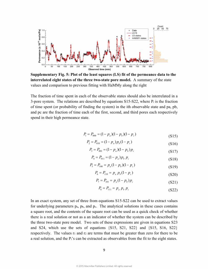
Supplementary Fig. 5: Plot of the least squares (LS) fit of the permeance data to the interrelated eight states of the three two-state pore model. A summary of the state values and comparison to previous fitting with HaMMy along the right The fraction of time spent in each of the observable states should also be interrelated in a 3-pore system. The relations are described by equations S15-S22, where Pi is the fraction of time spent (or probability of finding the system) in the ith observable state and pa, pb, and pc are the fraction of time each of the first, second, and third pores each respectively spend in their high permeance state.

1 000 (1 )(1 )(1 )a b cP P p p p (S15)

2 010 (1 ) (1 )a b cP P p p p (S16)

3 001 (1 )(1 )a b cP P p p p (S17)

4 011 (1 )a b cP P p p p (S18)

5 100 (1 )(1 )a b cP P p p p (S19)

6 110 (1 )a b cP P p p p (S20)

7 101 (1 )a b cP P p p p (S21)

8 111 a b cP P p p p (S22) In an exact system, any set of three from equations S15-S22 can be used to extract values for underlying parameters pa, pb, and pc. The analytical solutions in these cases contains a square root, and the contents of the square root can be used as a quick check of whether there is a real solution or not as a an indicator of whether the system can be described by the three two-state pore model. Two sets of these expressions are given in equations S23 and S24, which use the sets of equations {S15, S21, S22} and {S15, S16, S22} respectively. The values r1 and r2 are terms that must be greater than zero for there to be a real solution, and the Pi’s can be extracted as observables from the fit to the eight states.


10

27 1

2 21 7 8 7 8 7184 ( ) ( (1 ) )r P P P P PP PP P (S23)

22 2 8 2 2 21 2 81 14 ( ) ( ( 1) ( ) )r P P P PP P PP P P (S24)

Calculation of these values with the data set collected using Ne gas yields r1=2*10-5 and r2=3*10-3; the positive values show that a real solution is possible based on those observed values. The two sets of equations, equation S14 and equations S15-S22, describe a result in an over specified system where the number of observable values and their equations is greater than the variables. Hence the fidelity of the observed data to the model of three two-state pores is best described in terms of a fit of the equations to their observed values in the experimental data. Rather than selecting a subset of the equations, the three underlying values of pa, pb, and pc were fit with least squares between the calculated Pi based on equations S15-S22 and the observed state times. The fitted values of pa, pb, and pc were found to be 0.381, 0.376, and 0.110 in order of increasing yi value. The comparison of the eight Pi values calculated with those fitted parameters to the observed values is represented in Supplementary Fig. 6.

Supplementary Fig. 6 Comparison of the values for fraction time spent, Pi, between the observed values from the experimental results and the values calculated from the three fitted parameters of the three two-state pore model.


11

The observed dwell times and corresponding fraction of time spent being fit well shows that the experimental membrane is consistent with a three pore model. Furthermore, we confirmed that similar simulated data with eight states, unconstrained by the three pore model, could not be fit as well as the experimental results.

9. Transition activation energy estimation

The frequency of transitions between states can be used to estimate the activation energy of the pore transitions. For Ne, the hidden Markov modelling identified 54 transitions that did not occur during the time between experimental runs. The total observed time was 785 minutes. Therefore, the frequency is about 1 transition per 15 min, or 1.1 x 10-3 1/s; with the assumption there are three active pores contributing to the fluctuations, the average frequency for an individual pore should be a factor of three less, 3.7x10-4 1/s. The kinetic rate constant is approximately equivalent to the frequency. For an elementary process, the kinetic rate constant consists of an attempt frequency, A, and an exponential dependence on activation energy.

4 13.7 10aE

RTk Ae s

(S25)

Molecular vibrations typically occur within a few orders of magnitude of 1013 1/s8.

Assuming a temperature of 298 K, the average activation energy for a transition, aE , can

be estimated as 1.0 eV.

10. Estimation of change in permeance due to pore rearrangement

We attribute the stochastic switching in permeance to small fluctuations at the pore site which affects the transmission probability. One possible source of fluctuations is reaction of the pore edge functionalization with atmospheric species while another is pore isomerization, in which the pore's bonds transition between stable chemical states through rearrangement, but no gain or loss of the atoms around the pore. Supplementary Fig. 7a illustrates a simple possible rearrangement: moving a single carbon atom in a model pore which excludes functionalization. The effective size is approximately the expected pore size based on the observed molecular sieving. Even for this simplified model, the small rearrangement results in a relatively significant change in the energy barrier, as shown in Supplementary Fig. 7b. That change in the model pore’s estimated energy barrier gives an expected change in the permeance of around a factor of two or three, which is consistent with the magnitude of the experimentally observed changes in Fig. 4. The sensitivity of the permeance to small rearrangements at a single pore further supports the hypothesis that a single pore (or a very small number of pores) is responsible for the observed gas transport in our measured porous graphene.


12

Supplementary Fig. 7 Atom rearrangement at pore mouth. (a) Representation of a simple model pore rearrangement. (b) Estimation of barrier energy for two pores depicted in (a) and the expected ratio of permeance between the two.

In Supplementary Fig. 7b, it is shown that a small rearrangement in the pore could result in a meaningful change in the barrier energy and the expected permeance. The ratio is derived from an alternate form of equation 2 in the main text rearranged in terms of permeance, θ. The transmission coefficient, γ, is expanded into a geometric area term, ag, and a barrier energy, Ea, term.

1 dn

dt 2π R 2π R

aERT

g

w w

a e

p M T M T

(S26)

When there is a pore rearrangement, both component terms of the effective pore area can change. However, as a first order approximation, we will assume that the geometric area term remains approximately constant. Therefore, the ratio of the permeances reported in Supplementary Fig. 4b is simply the following:

,2 ,2

,1 ,1

,22

1,1

~

a a

a a

E ERT RT

g

E ERT RT

g

a e e

a e e

(S27)

The energy barriers for pore configuration 1, ,1aE , and pore configuration 2, ,2aE , are

calculated using a single-centre Lennard-Jones potential with the following parameters.

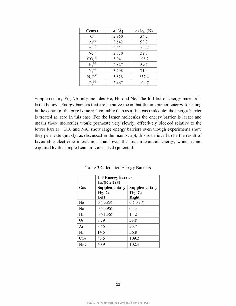
TABLE 2 Parameters for Lennard-Jones potential calculation


13

Center σ (Å) ϵ / kB (K) C9 2.960 34.2

Ar10 3.542 93.3 He10 2.551 10.22 Ne10 2.820 32.8

CO210 3.941 195.2

H210 2.827 59.7

N210 3.798 71.4

N2O10 3.828 232.4

O210 3.467 106.7

Supplementary Fig. 7b only includes He, H2, and Ne. The full list of energy barriers is listed below. Energy barriers that are negative mean that the interaction energy for being in the centre of the pore is more favourable than as a free gas molecule; the energy barrier is treated as zero in this case. For the larger molecules the energy barrier is larger and means those molecules would permeate very slowly, effectively blocked relative to the lower barrier. CO2 and N2O show large energy barriers even though experiments show they permeate quickly; as discussed in the manuscript, this is believed to be the result of favourable electronic interactions that lower the total interaction energy, which is not captured by the simple Lennard-Jones (L-J) potential.

Table 3 Calculated Energy Barriers

L-J Energy barrier Ea/(R x 298)

Gas Supplementary Fig. 7a Left

Supplementary Fig. 7a Right

He 0 (-0.83) 0 (-0.37)

Ne 0 (-0.96) 0.73

H2 0 (-1.36) 1.12

O2 7.29 23.8

Ar 8.55 25.7

N2 14.5 36.8

CO2 45.5 109.2

N2O 40.9 102.4


14

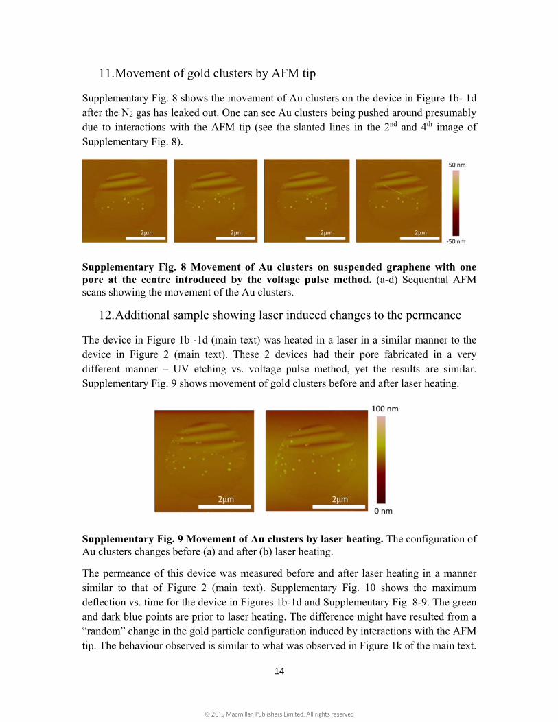
11. Movement of gold clusters by AFM tip

Supplementary Fig. 8 shows the movement of Au clusters on the device in Figure 1b- 1d after the N2 gas has leaked out. One can see Au clusters being pushed around presumably due to interactions with the AFM tip (see the slanted lines in the 2nd and 4th image of Supplementary Fig. 8).

Supplementary Fig. 8 Movement of Au clusters on suspended graphene with one pore at the centre introduced by the voltage pulse method. (a-d) Sequential AFM scans showing the movement of the Au clusters.

12. Additional sample showing laser induced changes to the permeance

The device in Figure 1b -1d (main text) was heated in a laser in a similar manner to the device in Figure 2 (main text). These 2 devices had their pore fabricated in a very different manner – UV etching vs. voltage pulse method, yet the results are similar. Supplementary Fig. 9 shows movement of gold clusters before and after laser heating.

Supplementary Fig. 9 Movement of Au clusters by laser heating. The configuration of Au clusters changes before (a) and after (b) laser heating.

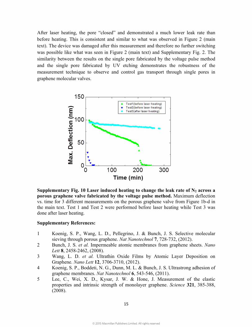
The permeance of this device was measured before and after laser heating in a manner similar to that of Figure 2 (main text). Supplementary Fig. 10 shows the maximum deflection vs. time for the device in Figures 1b-1d and Supplementary Fig. 8-9. The green and dark blue points are prior to laser heating. The difference might have resulted from a “random” change in the gold particle configuration induced by interactions with the AFM tip. The behaviour observed is similar to what was observed in Figure 1k of the main text.


15

After laser heating, the pore “closed” and demonstrated a much lower leak rate than before heating. This is consistent and similar to what was observed in Figure 2 (main text). The device was damaged after this measurement and therefore no further switching was possible like what was seen in Figure 2 (main text) and Supplementary Fig. 2. The similarity between the results on the single pore fabricated by the voltage pulse method and the single pore fabricated by UV etching demonstrates the robustness of the measurement technique to observe and control gas transport through single pores in graphene molecular valves.

Supplementary Fig. 10 Laser induced heating to change the leak rate of N2 across a porous graphene valve fabricated by the voltage pulse method. Maximum deflection vs. time for 3 different measurements on the porous graphene valve from Figure 1b-d in the main text. Test 1 and Test 2 were performed before laser heating while Test 3 was done after laser heating.

Supplementary References:

1 Koenig, S. P., Wang, L. D., Pellegrino, J. & Bunch, J. S. Selective molecular sieving through porous graphene. Nat Nanotechnol 7, 728-732, (2012).

2 Bunch, J. S. et al. Impermeable atomic membranes from graphene sheets. Nano Lett 8, 2458-2462, (2008).

3 Wang, L. D. et al. Ultrathin Oxide Films by Atomic Layer Deposition on Graphene. Nano Lett 12, 3706-3710, (2012).

4 Koenig, S. P., Boddeti, N. G., Dunn, M. L. & Bunch, J. S. Ultrastrong adhesion of graphene membranes. Nat Nanotechnol 6, 543-546, (2011).

5 Lee, C., Wei, X. D., Kysar, J. W. & Hone, J. Measurement of the elastic properties and intrinsic strength of monolayer graphene. Science 321, 385-388, (2008).


16

6 Jin, H., Heller, D. A., Kim, J. -H. & Strano, M. S. Stochastic Analysis of Stepwise Fluorescence Quenching Reactions on Single-Walled Carbon Nanotubes: Single Molecule Sensors. Nano letters 8, 4299-4304, (2008).

7 McKinney, S. A., Joo, C. & Ha, T. Analysis of single-molecule FRET trajectories using hidden Markov modeling. Biophys J 91, 1941-1951, (2006).

8 Kolasinski, K. W. Surface Science: Foundations of Catalysis and Nanoscience. (Wiley, 2008).

9 Steele, W. A. The Interaction of Gases with Solid Surfaces. (Pergamon Press, 1974).

10 Reid, R. C., Prausnitz, J. M. & Poling, B. E. The Properties of Gases and Liquids. (McGraw-Hill, 1987).


Documents

Molecular valves for controlling gas phase transport made