Molecular dynamics meets the physical world:Thermostats and barostats

Justin Finnertyj.finnerty@grs-sim.de, 2011

Scientific theories of physical world

•Energy is invariant

•Real world has quantum selection rules

•E = PV/nRT

•With constant energy we have PV = nRT

Molecular dynamics reviewPhase-space and trajectories

• State of classical system (canonical): described by position and momenta of all particles (notation q is position and p is momentum).

• Phase space point X = (q,p) gives 6N degrees of freedom

• Extract property from ensemble

• Intractable to evaluate over phase space

• N = 100; q, p assume +1,-1 in each coordinate; 26N ≅ 4x10180 calc of A and E

�A� =

� �A(q,p)P (q,p)dqdp

P (q,p) = Q−1e−E(q,p)/kBT

Q =

� �e−E(q,p)/kBT dqdp

Molecular dynamics reviewProperties of ensemble average

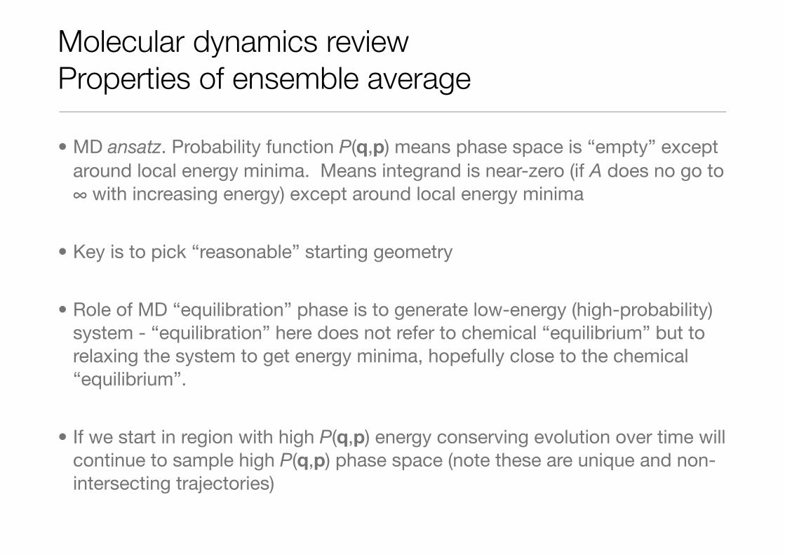
• MD ansatz. Probability function P(q,p) means phase space is “empty” except around local energy minima. Means integrand is near-zero (if A does no go to ∞ with increasing energy) except around local energy minima

• Key is to pick “reasonable” starting geometry

• Role of MD “equilibration” phase is to generate low-energy (high-probability) system - “equilibration” here does not refer to chemical “equilibrium” but to relaxing the system to get energy minima, hopefully close to the chemical “equilibrium”.

• If we start in region with high P(q,p) energy conserving evolution over time will continue to sample high P(q,p) phase space (note these are unique and non-intersecting trajectories)

Molecular dynamics reviewTime average of trajectories

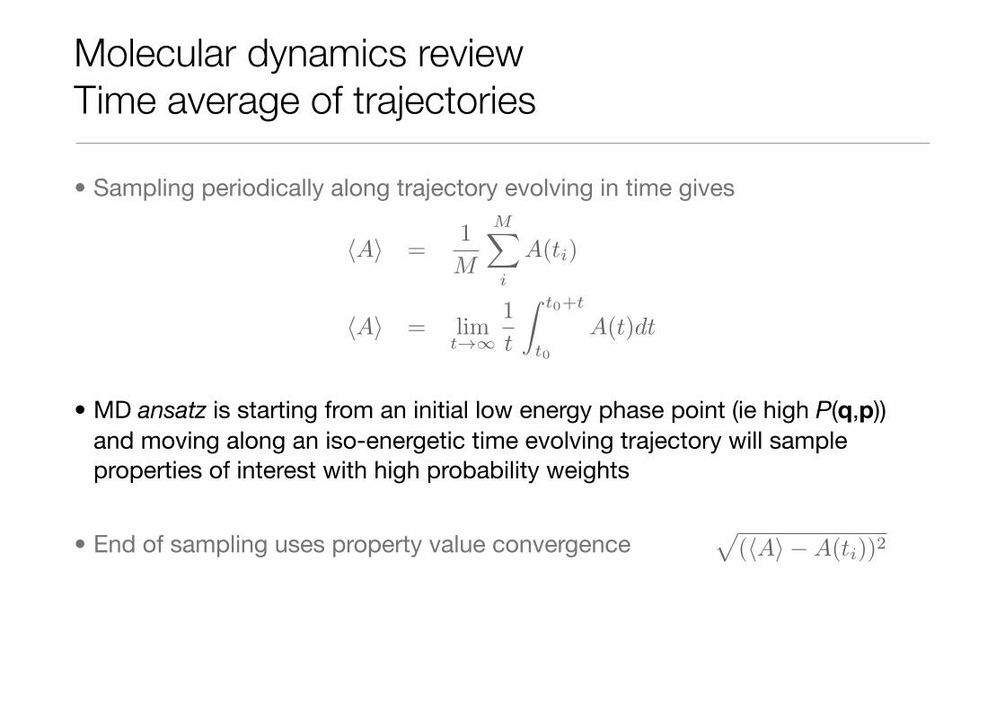
• Sampling periodically along trajectory evolving in time gives

• MD ansatz is starting from an initial low energy phase point (ie high P(q,p)) and moving along an iso-energetic time evolving trajectory will sample properties of interest with high probability weights

• End of sampling uses property value convergence

�A� =1

M

M�

i

A(ti)

�A� = limt→∞

1

t

� t0+t

t0

A(t)dt

�(�A� −A(ti))2

• Pressure (F is pairwise potential function):

•

• Temperature:

•

• Volume:

• parameters of the unit cell

Molecular dynamics reviewpressure, temperature, volume

T =1

3NkB

N�

i=1

|pi|2

mi

P =1

V

1

3

N�

i

N�

j>i

Fij |qi − qj |+|pi|mi

Physically important conditions

• Basic MD is constant energy: micro-canonical nVE

• Constant temperature (volume and/or pressure vary) : nVT

• Biological reactions

• Constant pressure (volume and/or temperature vary) : nPT

• Chemical reaction occurring open to the atmosphere

Control of system variables to maintain temperature or pressure

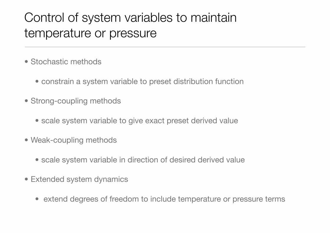
• Stochastic methods

• constrain a system variable to preset distribution function

• Strong-coupling methods

• scale system variable to give exact preset derived value

• Weak-coupling methods

• scale system variable in direction of desired derived value

• Extended system dynamics

• extend degrees of freedom to include temperature or pressure terms

Thermostat

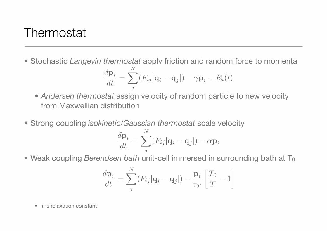
• Stochastic Langevin thermostat apply friction and random force to momenta

• Andersen thermostat assign velocity of random particle to new velocity from Maxwellian distribution

• Strong coupling isokinetic/Gaussian thermostat scale velocity

• Weak coupling Berendsen bath unit-cell immersed in surrounding bath at T0

• τ is relaxation constant

dpi

dt=

N�

j

(Fij |qi − qj |)− γpi +Ri(t)

dpi

dt=

N�

j

(Fij |qi − qj |)− αpi

dpi

dt=

N�

j

(Fij |qi − qj |)−pi

τT

�T0

T− 1

�

Nosé-Hoover thermostat

• Hoover, Phys. Rev. A 31 (1985) 1695; S. Nosé, J. Chem. Phys. 81 (1984) 511; S. Nosé, Mol. Phys. 52 (1984) 255

• add extra term η to the equations of motion

• The Q can be considered to be some fictional “heat bath mass”. Large Q gives weak coupling, Nosé suggested Q ~ 6nkBT

• temperature is second-order differential

dp

dt=

N�

i

N�

j>i

Fij |qi − qj |−pη

Qp

dpη

dt=

N�

i

|pi|2

2mi− 3

2nkBT

Example temperature control6.5 Controlling the system 203

0 1 2 3 4 5t*

1

1.1

1.2

1.3

1.4

T (!

/kB)

LDBerendsenNoséHoover

Figure 6.12 The temperature response of a Lennard–Jones fluid under control ofthree thermostats (solid line: Langevin; dotted line: weak-coupling; dashed line:Nose–Hoover) after a step change in the reference temperature (Hess, 2002a, andby permission from van der Spoel et al., 2005.)

p!M =p2

!M!1

QM!1! kBT. (6.135)

6.5.5 Comparison of thermostats

A comparison of the behavior in their approach to equilibrium of the Lange-vin, weak-coupling and Nose–Hoover thermostats has been made by Hess(2002a). Figure 6.12 shows that – as expected – the Nose–Hoover thermo-stat shows oscillatory behavior, while both the Langevin and weak-couplingthermostats proceed with a smooth exponential decay. The Nose–Hooverthermostat is therefore much less suitable to approach equilibrium, but it ismore reliable to produce a canonical ensemble, once equilibrium has beenreached.

D’Alessandro et al. (2002) compared the Nose–Hoover, weak-couplingand Gaussian isokinetic thermostats for a system of butane molecules, cov-ering a wide temperature range. They conclude that at low temperaturesthe Nose–Hoover thermostat cannot reproduce expected values of thermo-dynamic variables as internal energy and specific heat, while the isokineticthermostat does. The weak-coupling thermostat reproduces averages quitewell, but has no predictive power from its fluctuations. These authors alsomonitored the Lyapunov exponent that is a measure of the rate at whichtrajectories deviate exponentially from each other; it is therefore an indica-

Nosé-Hoover thermostat

• Energy (Hamiltonian H) of the simulated (physical) system fluctuates. However, the energy of the system + heat bath (Hamiltonian H’) is conserved

• If the system is ergodic the stationary state can then be shown to be a canonical distribution

H� = H +

Q

2p2η + 3nkBTf(pη)

exp

�−β

�V +

p2

2m+

Q

2p2η

��

Barostats

• Weak coupling Berendsen bath

• scale each dimension by μ: where β is isothermal compressibility - don’t need to know exactly as it appears as ratio with τ (a relaxation constant)

• This is similar to the Berendsen thermostat where we scale velocities by λ.

• Together give realistic fluctuations in T and P (J. Chem. Phys. 81 (1984) 3684)

• Note: pressure scale dimension, temperature scale velocity

µ =

�1− β∂t

τ(P0 − P )

�1/3P =

1

V

1

3

N�

i

N�

j>i

Fij |qi − qj |+|pi|mi

λ =

�1 +

∂t

τ

�T0

T− 1

��1/2

Berendson barostat

Instantaneous pressure vs time and instantaneous temperature vs time in an MD simulation of 256 particles at a density of 0.8442, using the Berendsen barostat to impose an instantaneous pressure jump from 1.0 to 6.0. Each

curve corresponds to a different value of the rise time constant τ

Parrinello-Rahman Barostat

• The extended dimension of Nosé-Hoover thermostat can be applied to pressure to give a Nosé-Hoover barostat

• The Parrinello-Rahman barostat (J. Appl. Phys. 52 (1981) 7182) extended this further by making each unit vector of the unit-cell independent so that

• as with Nosé-Hoover the volume is a variable in the simulation.

• additionally allows dynamic shape change (gives control of stress as well as pressure)

• The additional terms in the equations of motion are of similar type to that shown for the Nosé-Hoover thermostat (though somewhat more complex!)

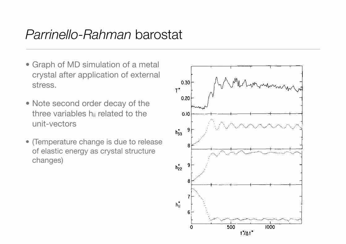
Parrinello-Rahman barostat

• Graph of MD simulation of a metal crystal after application of external stress.

• Note second order decay of the three variables hii related to the unit-vectors

• (Temperature change is due to release of elastic energy as crystal structure changes)

state was easy to demonstrate. Using the end of the above .xTI = 15, T* = 0.14 equilibrium run as the initial condi-tion, the load was reduced to.x TI = 0 in several short runs with successively smaller values of.x TI , the temperature in the final.x TI = 0 run being T * = 0.14. Finally, on reaching a no load condition, the system was quenched to a very low temperature to observe the pair correlation with the effects of thermal motion removed. 12 This is shown in Fig. 2(b) leav-ing no doubt that one has regained the original perfect fcc structure. Of course, all other indicators, namely the compo-nents of h*, pointed to the same conclusion.

c. Structure transformation under further compression

After completing the .x TI = 15 study the load was raised to.x Tl = 20 and the dynamics was allowed to take its course according to the dictates of the equations of motion [Eqs. (2.9) and (2.25)].

The behavior of the system was remarkably different as might have been guessed by the title given to this subsection. Figure 3 shows the details of the changes with the passage of time. The MD cell, i.e., the h matrix, undergoes large and swift changes which cannot possibly be described as elastic deformations. In fact, as Fig. 3 shows, when equilibrium was reached the average values of the components of h* were (h Tl) = 5.54 ± 0.03, (h!2) = 9.76 ± 0.06,

................. , ............................. "' ...... .

8

7

6 ...................... ........... .......... ''' ............. " ... ...... . ........... .

o 500 1000

FIG. 3. Behavior of the MD cell parameters and the temperature of the system as it evolves in time when the compressive [100] load is increased fromIf. = + 15 to + 20 (the latter value shown in Fig. I). After a rapid change h settle down to values at which an hcp structure can be accommodated in the MD cell (Fig. 2(c) shows the gIrl at the end of the above time elapse). The rise in temperature is due to the release of elastic energy as the transformation occurs. See Sec. C for details.

7187 J. Appl. Phys., Vol. 52. No. 12, December 1981

(h f3) = 9.18 ± 0.09. The average of the nondiagonal ele-ments was essentially zero. We note here that the tetragonal symmetry of the initially stressed state is destroyed as a re-sult of this transformation; one gets instead an orthorhombic system, still under [100] compression. (See below for the de-scription of this orthorhombic system under zero load.)

As seen in Fig. 3, contemporaneously with the rapid changes in h*, the temperature T * increased from - 0.15 to -0.30, finally settling down to -0.25 or perhaps somewhat less. This is obviously a manifestation of an abrupt release of elastic energy in the relatively short time interval of -100.at * (or -0.4 psI. Of course we recall that the .x Tl = 15 to 20 change was made in one L1 t *.

The pair correlation at the end of the .x Tl = 20 run is shown in Fig. 2(c). In spite of the large deformations in h mentioned above, theg(r) in Fig. 2(c) is very similar to the one in Fig. 2(a) and does not show clear evidence of a new ar-rangement of particles. However, the quenching technique does indicate that a new structure has been formed. The gIrl after quenching is shown in Fig. 2(d). This figure displays not only the shell structure of a hexagonal close packed system but it also shows that under this loaded state otherwise single shells show up as split into two. Visual examination of part i-cle positions suitably displayed showed that stacking faults were present in the hcp arrangement. It is interesting to note here that the direction of the compressive stress is normal to the c axis of the new, close-packed structure.

Having obtained the above-described transformation under a compressive load we reduced the load from .x TI = 20 to .x Tl = 0 using several intermediate steps. The temperature in the final.x Tl = 0 run was T * = 0.21. There was no structural change evident during this process. To re-veal the structure clearly at the end of this process (of reduc-ing the load from a high value to zero) we used the usual quench technique. The gIrl is shown in Fig. 2(e). The shell

• 0 • 0 0 o

0 • 0

• •

6 0

ffi • 0 o

(a) (h) (e)

[010] L [100]

FIG. 4. Two planes of an fcc structure perpendicular to [00 I] are shown by o and. respectively. (a)-(b) shows how the face-centered square structure changes to a triangular lattice on suitable compression in the [100] direc-tion. (b)-(c) shows the necessary translation of the. planes to achieve hcp ordering. At the same time spacing between 0 and. planes has to corre-spond to the "c/a" value of an hcp arrangement. namely v8/3.

M. Parrinello and A. Rahman 7187

Downloaded 20 Jan 2011 to 134.94.14.60. Redistribution subject to AIP license or copyright; see http://jap.aip.org/about/rights_and_permissions

Consequences of control method

method pro con

stochastic canonical disturb dynamics

strong coupling canonical in phase spacenon-Hamiltoniandisturb dynamic

accuracy

weak couplingno well-defined ensemblegood for non-equilibrium

ensemble average okperturbation not ok

extended dynamicscanonical in configuration

spacemore computationdisturb dynamics

Consequences of control method

method pro con

Berendsen thermostat and barostat

fast, smooth first-order approach to equilibrium

now considered less reliable for simulation at

equilibrium

Nosé-Hoover thermostat and Parinello-Rahman

barostat

maintain canonical ensemble.

considered most reliable for simulation at

equilibrium and for predicting thermo-dynamic properties

slow, second-order approach to equilibrium

• What impacts will the different control methods have on parallel MD code? (steps in right square not necessarily shown in actual order)

• Pressure and temperature are global properties calculated as ensemble averages

Group discussion: MD calculation process

equilibrate

pass end condition

experiment

pass start condition

solve equations of motion

propagate ensemble

sample

apply control