Embed Size (px)
Citation preview
Molecular Dynamics Simulationsin GROMACS
presented by
Jan Schulze
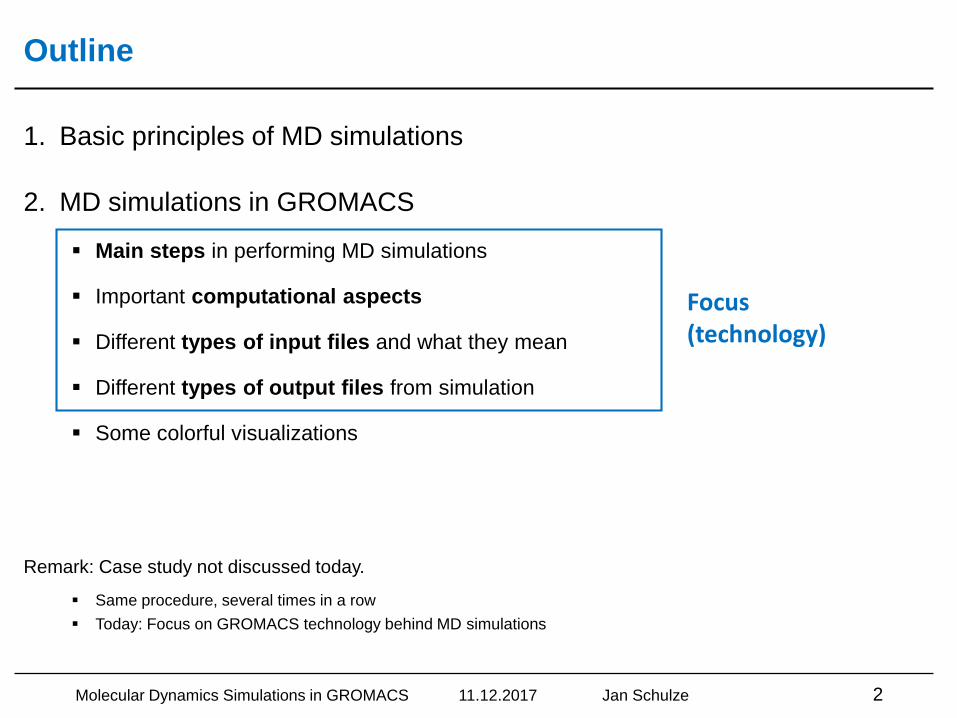
Outline
1. Basic principles of MD simulations
2. MD simulations in GROMACS
▪ Main steps in performing MD simulations
▪ Important computational aspects
▪ Different types of input files and what they mean
▪ Different types of output files from simulation
▪ Some colorful visualizations
Remark: Case study not discussed today.
▪ Same procedure, several times in a row
▪ Today: Focus on GROMACS technology behind MD simulations
Molecular Dynamics Simulations in GROMACS 11.12.2017 Jan Schulze 2
Focus(technology)
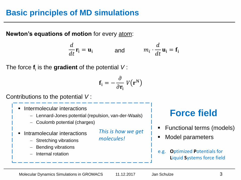
Basic principles of MD simulations
Newton’s equations of motion for every atom:
The force fi is the gradient of the potential V :
Contributions to the potential V :
▪ Intermolecular interactions
Lennard-Jones potential (repulsion, van-der-Waals)
Coulomb potential (charges)
▪ Intramolecular interactions
Stretching vibrations
Bending vibrations
Internal rotation
Molecular Dynamics Simulations in GROMACS 11.12.2017 Jan Schulze 3
𝑑
𝑑𝑡𝐫i = 𝐮i 𝑚𝑖 ⋅
𝑑
𝑑𝑡𝐮i = 𝐟iand
𝐟i = −𝜕
𝜕𝐫i𝑉 𝐫N
▪ Functional terms (models)
▪ Model parameters
Force field
This is how we get molecules!
e.g. Optimized Potentials for Liquid Systems force field
t1
Δ𝐫1Δ𝐫2
Δ𝐫3Δ𝐫𝑁
Δ𝐫1Δ𝐫2
Δ𝐫3Δ𝐫𝑁
t2 t3
V(r1,…,rN) V(r1,…,rN)
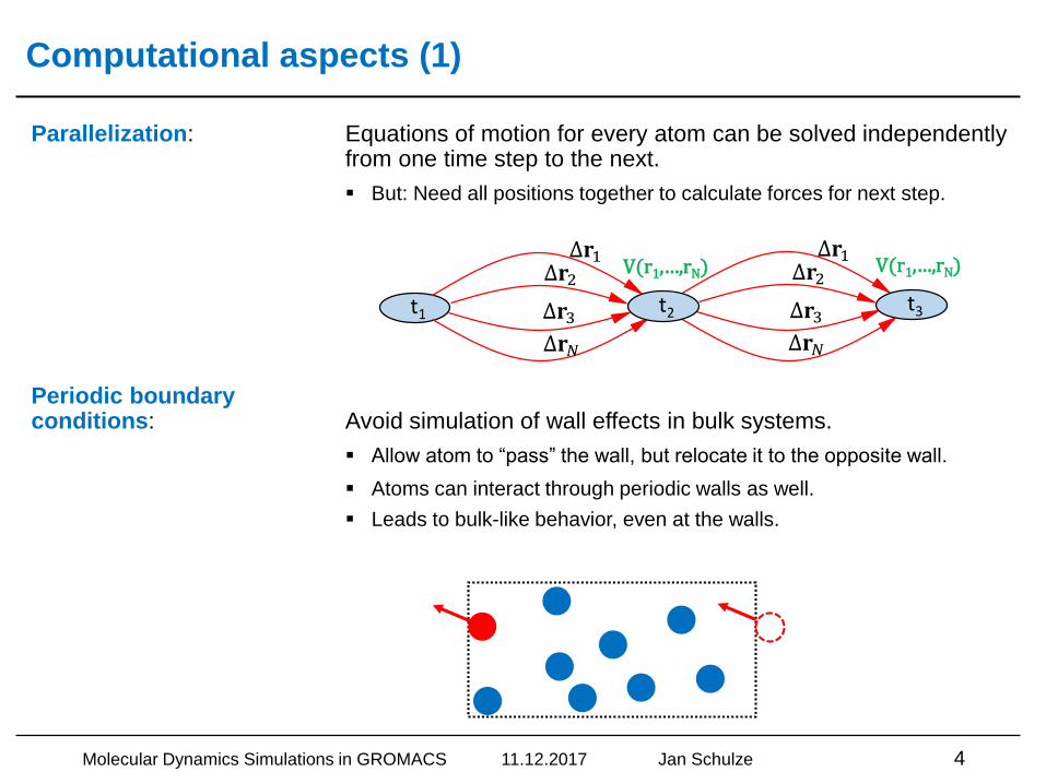
Parallelization: Equations of motion for every atom can be solved independently from one time step to the next.
▪ But: Need all positions together to calculate forces for next step.
Periodic boundaryconditions: Avoid simulation of wall effects in bulk systems.
▪ Allow atom to “pass” the wall, but relocate it to the opposite wall.
▪ Atoms can interact through periodic walls as well.
▪ Leads to bulk-like behavior, even at the walls.
Computational aspects (1)
Molecular Dynamics Simulations in GROMACS 11.12.2017 Jan Schulze 4
Computational aspects (2)
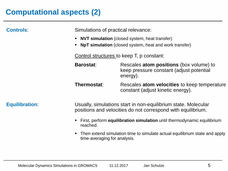
Controls: Simulations of practical relevance:
▪ NVT simulation (closed system, heat transfer)
▪ NpT simulation (closed system, heat and work transfer)
Control structures to keep T, p constant:
Barostat: Rescales atom positions (box volume) to keep pressure constant (adjust potential energy).
Thermostat: Rescales atom velocities to keep temperature constant (adjust kinetic energy).
Equilibration: Usually, simulations start in non-equilibrium state. Molecular positions and velocities do not correspond with equilibrium.
▪ First, perform equilibration simulation until thermodynamic equilibrium reached.
▪ Then extend simulation time to simulate actual equilibrium state and apply time-averaging for analysis.
Molecular Dynamics Simulations in GROMACS 11.12.2017 Jan Schulze 5
Computational aspects (3)
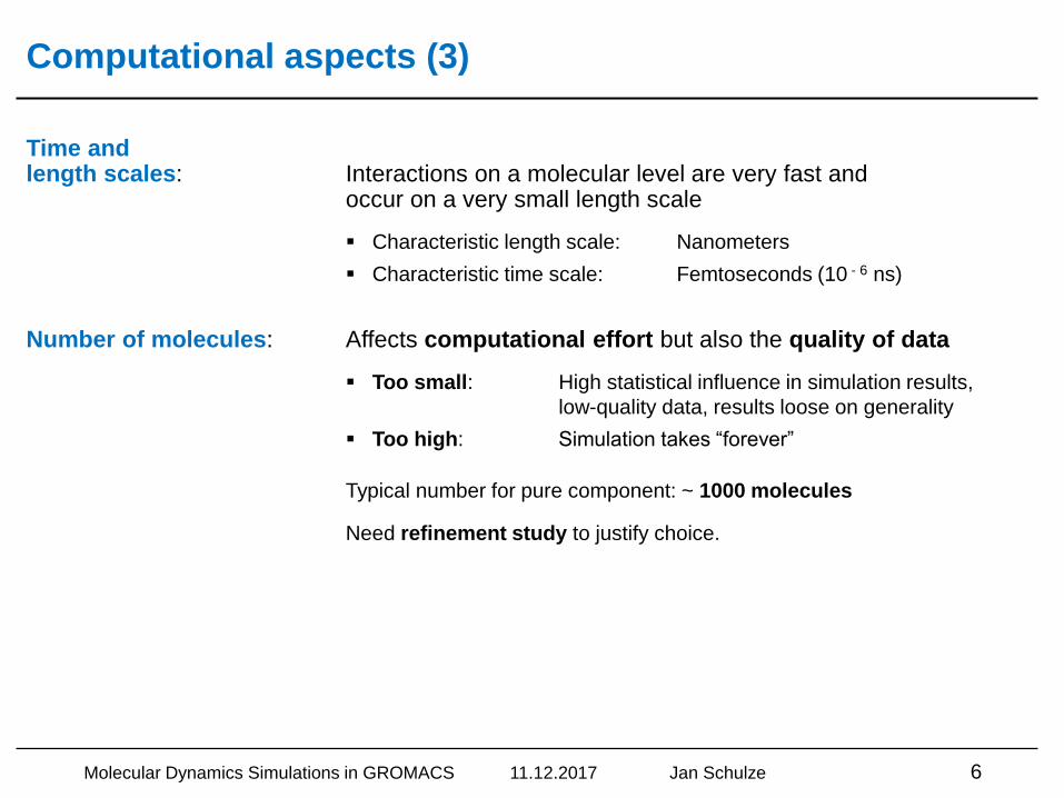
Time and length scales: Interactions on a molecular level are very fast and
occur on a very small length scale
▪ Characteristic length scale: Nanometers
▪ Characteristic time scale: Femtoseconds (10 - 6 ns)
Number of molecules: Affects computational effort but also the quality of data
▪ Too small: High statistical influence in simulation results,
low-quality data, results loose on generality
▪ Too high: Simulation takes “forever”
Typical number for pure component: ~ 1000 molecules
Need refinement study to justify choice.
Molecular Dynamics Simulations in GROMACS 11.12.2017 Jan Schulze 6
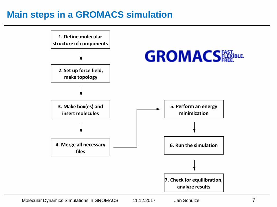
Main steps in a GROMACS simulation
Molecular Dynamics Simulations in GROMACS 11.12.2017 Jan Schulze 7
6. Run the simulation
7. Check for equilibration,
analyze results
1. Define molecular
structure of components
2. Set up force field,make topology
3. Make box(es) and
insert molecules
4. Merge all necessary
files
5. Perform an energy
minimization
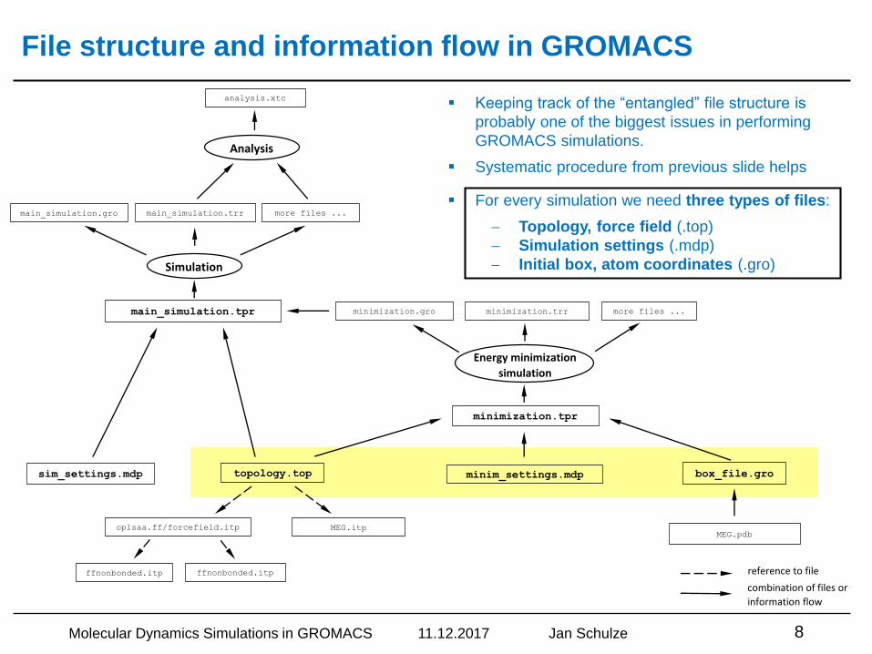
File structure and information flow in GROMACS
Molecular Dynamics Simulations in GROMACS 11.12.2017 Jan Schulze 8
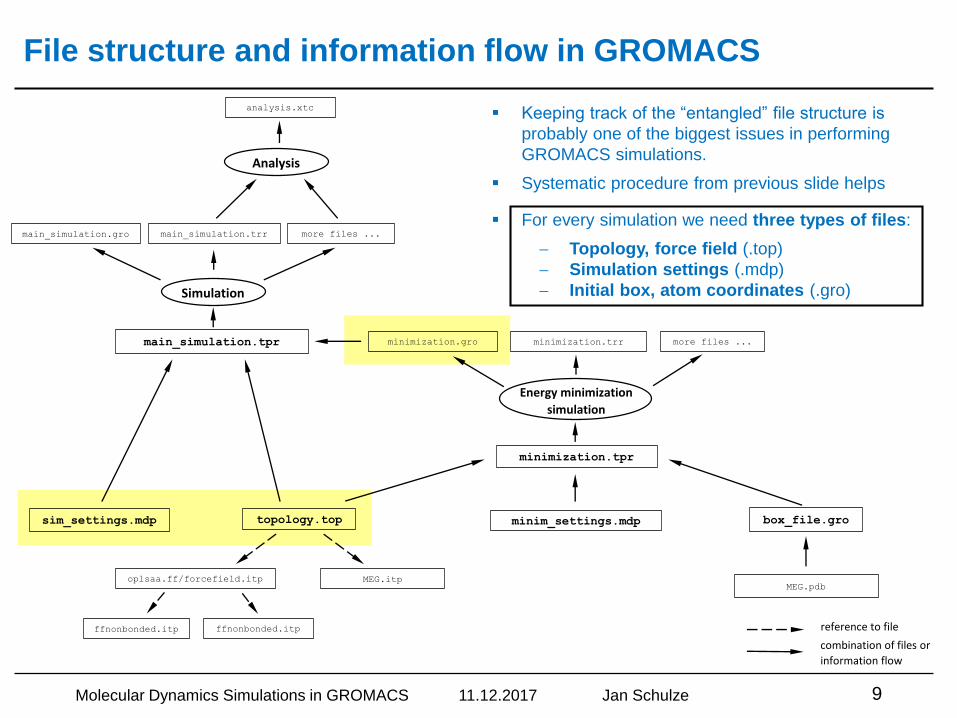
▪ Keeping track of the “entangled” file structure is
probably one of the biggest issues in performing
GROMACS simulations.
▪ Systematic procedure from previous slide helps
▪ For every simulation we need three types of files:
Topology, force field (.top)
Simulation settings (.mdp)
Initial box, atom coordinates (.gro)
topology.top
MEG.itpoplsaa.ff/forcefield.itp
ffnonbonded.itp ffnonbonded.itp reference to file
combination of files or
information flow
MEG.pdb
box_file.grominim_settings.mdp
minimization.tpr
Energy minimization
simulation
minimization.gro minimization.trr more files ...
Simulation
main_simulation.gro main_simulation.trr more files ...
main_simulation.tpr
sim_settings.mdp
Analysis
analysis.xtc
File structure and information flow in GROMACS
Molecular Dynamics Simulations in GROMACS 11.12.2017 Jan Schulze 9
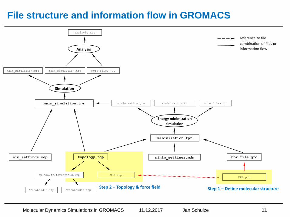
▪ Keeping track of the “entangled” file structure is
probably one of the biggest issues in performing
GROMACS simulations.
▪ Systematic procedure from previous slide helps
▪ For every simulation we need three types of files:
Topology, force field (.top)
Simulation settings (.mdp)
Initial box, atom coordinates (.gro)
topology.top
MEG.itpoplsaa.ff/forcefield.itp
ffnonbonded.itp ffnonbonded.itp reference to file
combination of files or
information flow
MEG.pdb
box_file.grominim_settings.mdp
minimization.tpr
Energy minimization
simulation
minimization.gro minimization.trr more files ...
Simulation
main_simulation.gro main_simulation.trr more files ...
main_simulation.tpr
sim_settings.mdp
Analysis
analysis.xtc
Step 1 – Define molecular structure of components
Molecular Dynamics Simulations in GROMACS 11.12.2017 Jan Schulze 10
1. Define molecular
structure of components
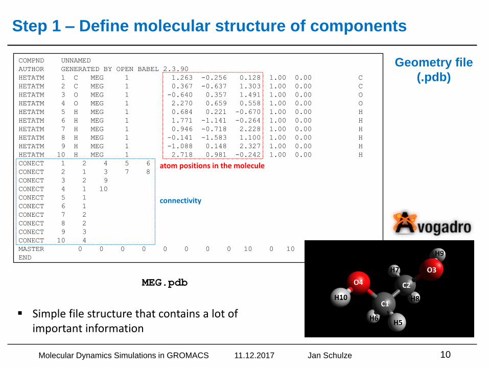
COMPND UNNAMED
AUTHOR GENERATED BY OPEN BABEL 2.3.90
HETATM 1 C MEG 1 1.263 -0.256 0.128 1.00 0.00 C
HETATM 2 C MEG 1 0.367 -0.637 1.303 1.00 0.00 C
HETATM 3 O MEG 1 -0.640 0.357 1.491 1.00 0.00 O
HETATM 4 O MEG 1 2.270 0.659 0.558 1.00 0.00 O
HETATM 5 H MEG 1 0.684 0.221 -0.670 1.00 0.00 H
HETATM 6 H MEG 1 1.771 -1.141 -0.264 1.00 0.00 H
HETATM 7 H MEG 1 0.946 -0.718 2.228 1.00 0.00 H
HETATM 8 H MEG 1 -0.141 -1.583 1.100 1.00 0.00 H
HETATM 9 H MEG 1 -1.088 0.148 2.327 1.00 0.00 H
HETATM 10 H MEG 1 2.718 0.981 -0.242 1.00 0.00 H
CONECT 1 2 4 5 6
CONECT 2 1 3 7 8
CONECT 3 2 9
CONECT 4 1 10
CONECT 5 1
CONECT 6 1
CONECT 7 2
CONECT 8 2
CONECT 9 3
CONECT 10 4
MASTER 0 0 0 0 0 0 0 0 10 0 10 0
END
MEG.pdb
atom positions in the molecule
connectivity
▪ Simple file structure that contains a lot of important information
Geometry file
(.pdb)
File structure and information flow in GROMACS
Molecular Dynamics Simulations in GROMACS 11.12.2017 Jan Schulze 11
Step 1 – Define molecular structureStep 2 – Topology & force field
topology.top
MEG.itpoplsaa.ff/forcefield.itp
ffnonbonded.itp ffnonbonded.itp
reference to file
combination of files or
information flow
MEG.pdb
box_file.grominim_settings.mdp
minimization.tpr
Energy minimization
simulation
minimization.gro minimization.trr more files ...
Simulation
main_simulation.gro main_simulation.trr more files ...
main_simulation.tpr
sim_settings.mdp
Analysis
analysis.xtc
Step 2 – Make topology
Molecular Dynamics Simulations in GROMACS 11.12.2017 Jan Schulze 12
1. Define molecular
structure of components
2. Set up force field,make topology
topology.top
oplsaa.ff/forcefield.itp
ffnonbonded.itp ffnonbonded.itp
Component_1.itp
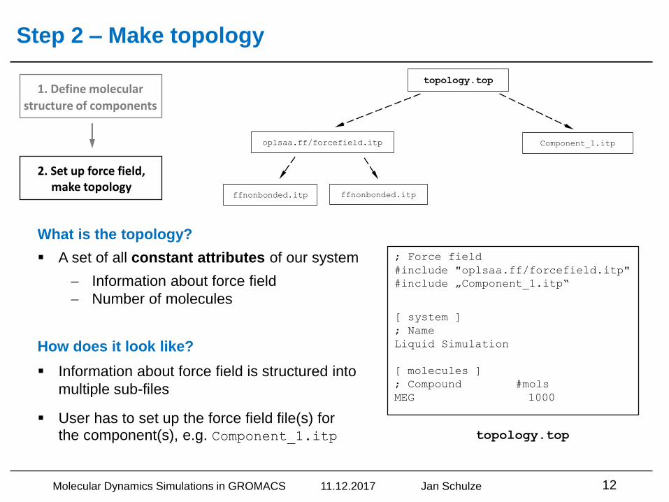
▪ Information about force field is structured into
multiple sub-files
▪ User has to set up the force field file(s) for the component(s), e.g. Component_1.itp
; Force field
#include "oplsaa.ff/forcefield.itp"
#include „Component_1.itp“
[ system ]
; Name
Liquid Simulation
[ molecules ]
; Compound #mols
MEG 1000
topology.top
What is the topology?
▪ A set of all constant attributes of our system
Information about force field
Number of molecules
How does it look like?
Step 2 – Set up force field
Molecular Dynamics Simulations in GROMACS 11.12.2017 Jan Schulze 13
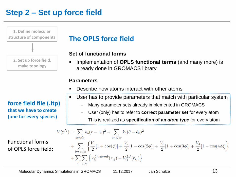
Set of functional forms
▪ Implementation of OPLS functional terms (and many more) is
already done in GROMACS library
Parameters
▪ Describe how atoms interact with other atoms
▪ User has to provide parameters that match with particular system
Many parameter sets already implemented in GROMACS
User (only) has to refer to correct parameter set for every atom
This is realized as specification of an atom type for every atom
The OPLS force field
force field file (.itp)that we have to create(one for every species)
Functional forms of OPLS force field:
1. Define molecular
structure of components
2. Set up force field,make topology
Step 2 – Set up force field
Molecular Dynamics Simulations in GROMACS 11.12.2017 Jan Schulze 14
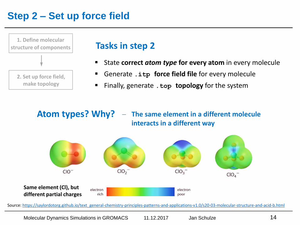
Source: https://saylordotorg.github.io/text_general-chemistry-principles-patterns-and-applications-v1.0/s20-03-molecular-structure-and-acid-b.html
▪ State correct atom type for every atom in every molecule
▪ Generate .itp force field file for every molecule
▪ Finally, generate .top topology for the system
Atom types? Why? The same element in a different molecule interacts in a different way
1. Define molecular
structure of components
2. Set up force field,make topology
Tasks in step 2
𝑉 𝑟12 = 𝑓 ⋅𝑞1 ⋅ 𝑞2𝑟12
Coulomb potential:
force field parameter(charge) of atom 2
force field parameter(charge) of atom 1
Same element (Cl), but different partial charges
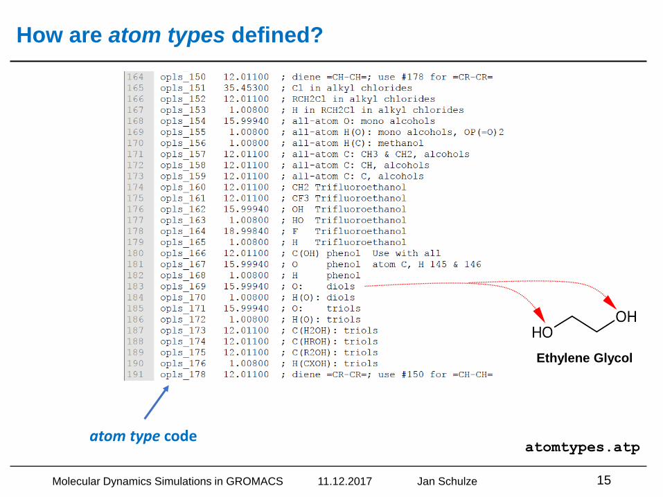
How are atom types defined?
Molecular Dynamics Simulations in GROMACS 11.12.2017 Jan Schulze 15
atom type codeatomtypes.atp
Ethylene Glycol
Molecular Dynamics Simulations in GROMACS 11.12.2017 Jan Schulze
[ moleculetype ]
; Name nrexcl
UNK 3
[ atoms ]
; nr type resnr residue atom cgnr charge mass
1 opls_800 1 UNK C00 1 -0.0329 12.0110
2 opls_801 1 UNK C01 1 -0.0330 12.0110
3 opls_802 1 UNK O02 1 -0.5898 15.9990
4 opls_803 1 UNK O03 1 -0.5898 15.9990
5 opls_804 1 UNK H04 1 0.1066 1.0080
6 opls_805 1 UNK H05 1 0.1066 1.0080
7 opls_806 1 UNK H06 1 0.1065 1.0080
8 opls_807 1 UNK H07 1 0.1065 1.0080
9 opls_808 1 UNK H08 1 0.4097 1.0080
10 opls_809 1 UNK H09 1 0.4097 1.0080
[ bonds ]
; i j funct
2 1 1 0.1529 224262.400
3 2 1 0.1410 267776.000
4 1 1 0.1410 267776.000
5 1 1 0.1090 284512.000
6 1 1 0.1090 284512.000
7 2 1 0.1090 284512.000
8 2 1 0.1090 284512.000
9 3 1 0.0945 462750.400
10 4 1 0.0945 462750.400
[ angles ]
; i j k funct c0
1 2 3 1 109.500 418.400
2 1 4 1 109.500 418.400
2 1 5 1 110.700 313.800
2 1 6 1 110.700 313.800
1 2 7 1 110.700 313.800
1 2 8 1 110.700 313.800
2 3 9 1 108.500 460.240
1 4 10 1 108.500 460.240
4 1 5 1 109.500 292.880
5 1 6 1 107.800 276.144
3 2 7 1 109.500 292.880
MEG
MEG
MEG
MEG
MEG
MEG
MEG
MEG
MEG
MEG
MEG
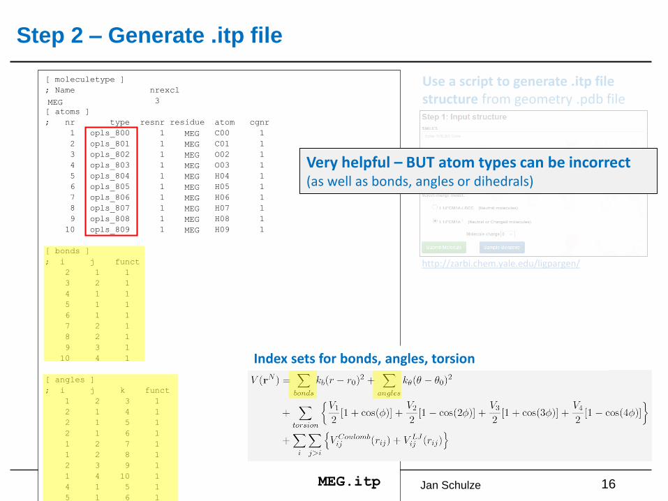
Step 2 – Generate .itp file
16MEG.itp
Index sets for bonds, angles, torsion
Use a script to generate .itp file structure from geometry .pdb file
http://zarbi.chem.yale.edu/ligpargen/
Browse…Very helpful – BUT atom types can be incorrect (as well as bonds, angles or dihedrals)
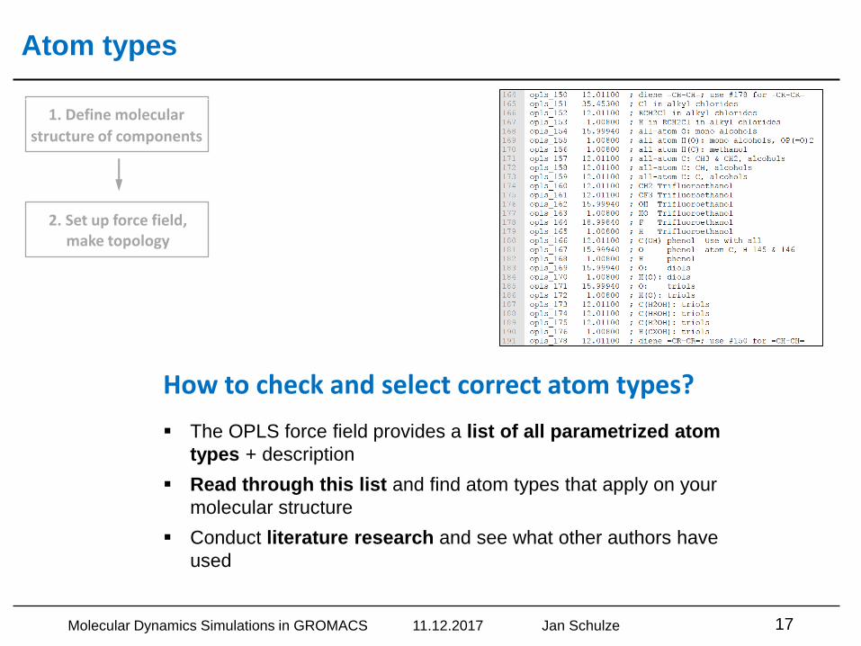
Atom types
Molecular Dynamics Simulations in GROMACS 11.12.2017 Jan Schulze 17
▪ The OPLS force field provides a list of all parametrized atom
types + description
▪ Read through this list and find atom types that apply on your
molecular structure
▪ Conduct literature research and see what other authors have
used
How to check and select correct atom types?
1. Define molecular
structure of components
2. Set up force field,make topology
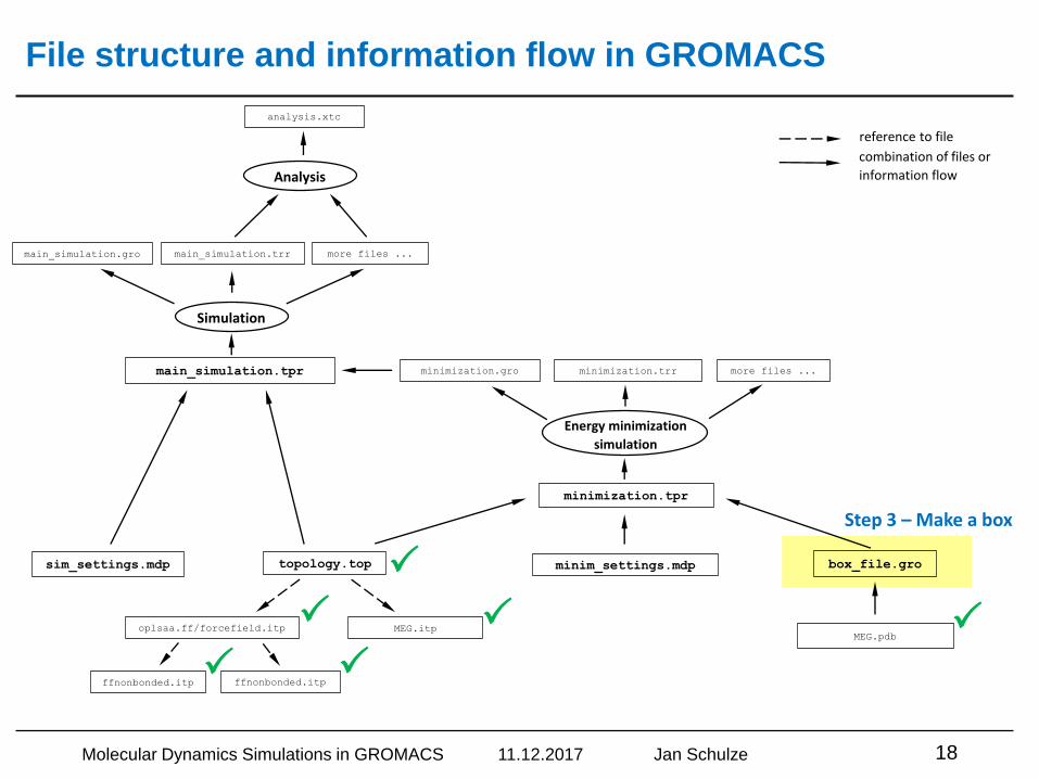
File structure and information flow in GROMACS
Molecular Dynamics Simulations in GROMACS 11.12.2017 Jan Schulze 18
topology.top
MEG.itpoplsaa.ff/forcefield.itp
ffnonbonded.itp ffnonbonded.itp
reference to file
combination of files or
information flow
MEG.pdb
box_file.grominim_settings.mdp
minimization.tpr
Energy minimization
simulation
minimization.gro minimization.trr more files ...
Simulation
main_simulation.gro main_simulation.trr more files ...
main_simulation.tpr
sim_settings.mdp
Analysis
analysis.xtc
PP
P
P
PP
Step 3 – Make a box
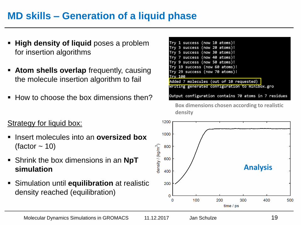
MD skills – Generation of a liquid phase
▪ High density of liquid poses a problem
for insertion algorithms
▪ Atom shells overlap frequently, causing
the molecule insertion algorithm to fail
▪ How to choose the box dimensions then?
Strategy for liquid box:
▪ Insert molecules into an oversized box
(factor ~ 10)
▪ Shrink the box dimensions in an NpT
simulation
▪ Simulation until equilibration at realistic
density reached (equilibration)
Molecular Dynamics Simulations in GROMACS 11.12.2017 Jan Schulze 19
Analysis
Box dimensions chosen according to realistic density
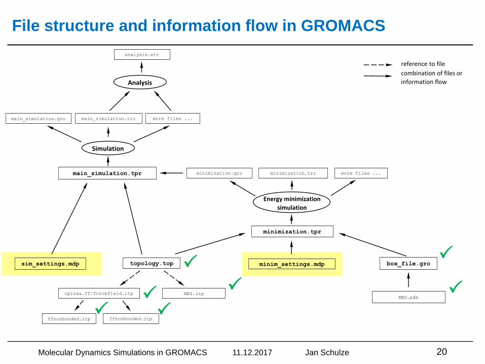
File structure and information flow in GROMACS
Molecular Dynamics Simulations in GROMACS 11.12.2017 Jan Schulze 20
topology.top
MEG.itpoplsaa.ff/forcefield.itp
ffnonbonded.itp ffnonbonded.itp
reference to file
combination of files or
information flow
MEG.pdb
box_file.grominim_settings.mdp
minimization.tpr
Energy minimization
simulation
minimization.gro minimization.trr more files ...
Simulation
main_simulation.gro main_simulation.trr more files ...
main_simulation.tpr
sim_settings.mdp
Analysis
analysis.xtc
P
P
P
P
P
PP
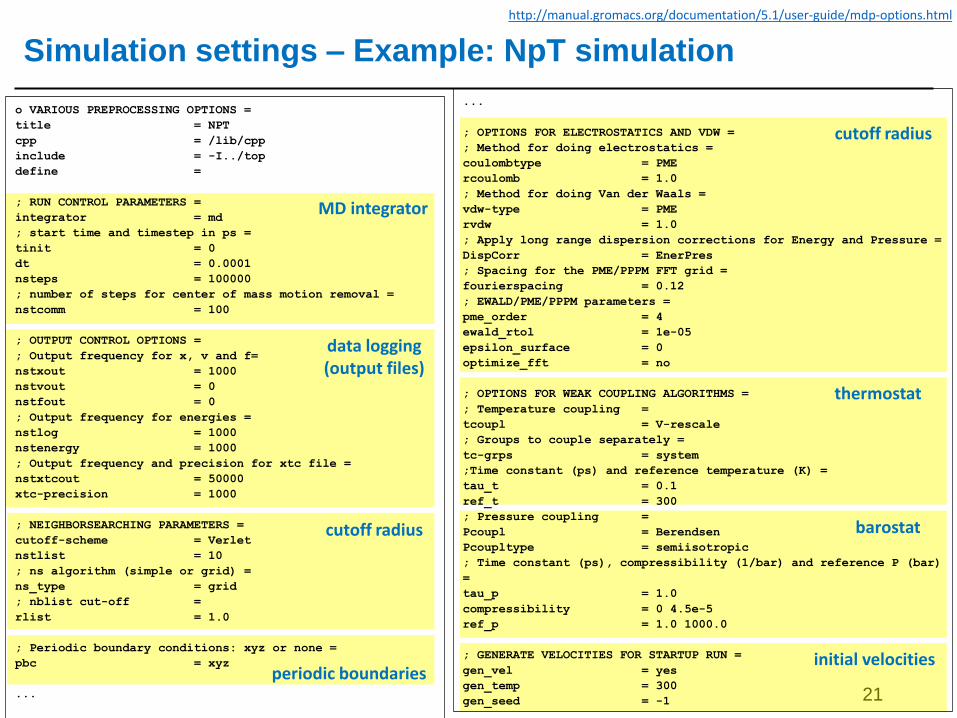
Simulation settings – Example: NpT simulation
21
MD integrator
data logging (output files)
cutoff radius
cutoff radius
periodic boundaries
thermostat
barostat
initial velocities
o VARIOUS PREPROCESSING OPTIONS =
title = NPT
cpp = /lib/cpp
include = -I../top
define =
; RUN CONTROL PARAMETERS =
integrator = md
; start time and timestep in ps =
tinit = 0
dt = 0.0001
nsteps = 100000
; number of steps for center of mass motion removal =
nstcomm = 100
; OUTPUT CONTROL OPTIONS =
; Output frequency for x, v and f=
nstxout = 1000
nstvout = 0
nstfout = 0
; Output frequency for energies =
nstlog = 1000
nstenergy = 1000
; Output frequency and precision for xtc file =
nstxtcout = 50000
xtc-precision = 1000
; NEIGHBORSEARCHING PARAMETERS =
cutoff-scheme = Verlet
nstlist = 10
; ns algorithm (simple or grid) =
ns_type = grid
; nblist cut-off =
rlist = 1.0
; Periodic boundary conditions: xyz or none =
pbc = xyz
...
...
; OPTIONS FOR ELECTROSTATICS AND VDW =
; Method for doing electrostatics =
coulombtype = PME
rcoulomb = 1.0
; Method for doing Van der Waals =
vdw-type = PME
rvdw = 1.0
; Apply long range dispersion corrections for Energy and Pressure =
DispCorr = EnerPres
; Spacing for the PME/PPPM FFT grid =
fourierspacing = 0.12
; EWALD/PME/PPPM parameters =
pme_order = 4
ewald_rtol = 1e-05
epsilon_surface = 0
optimize_fft = no
; OPTIONS FOR WEAK COUPLING ALGORITHMS =
; Temperature coupling =
tcoupl = V-rescale
; Groups to couple separately =
tc-grps = system
;Time constant (ps) and reference temperature (K) =
tau_t = 0.1
ref_t = 300
; Pressure coupling =
Pcoupl = Berendsen
Pcoupltype = semiisotropic
; Time constant (ps), compressibility (1/bar) and reference P (bar)
=
tau_p = 1.0
compressibility = 0 4.5e-5
ref_p = 1.0 1000.0
; GENERATE VELOCITIES FOR STARTUP RUN =
gen_vel = yes
gen_temp = 300
gen_seed = -1
http://manual.gromacs.org/documentation/5.1/user-guide/mdp-options.html
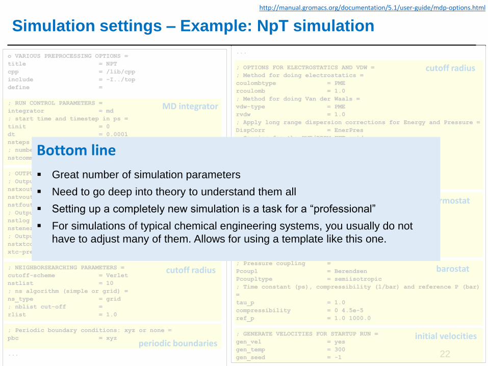
Simulation settings – Example: NpT simulation
22
MD integrator
data logging (output files)
cutoff radius
cutoff radius
periodic boundaries
thermostat
barostat
initial velocities
o VARIOUS PREPROCESSING OPTIONS =
title = NPT
cpp = /lib/cpp
include = -I../top
define =
; RUN CONTROL PARAMETERS =
integrator = md
; start time and timestep in ps =
tinit = 0
dt = 0.0001
nsteps = 100000
; number of steps for center of mass motion removal =
nstcomm = 100
; OUTPUT CONTROL OPTIONS =
; Output frequency for x, v and f=
nstxout = 1000
nstvout = 0
nstfout = 0
; Output frequency for energies =
nstlog = 1000
nstenergy = 1000
; Output frequency and precision for xtc file =
nstxtcout = 50000
xtc-precision = 1000
; NEIGHBORSEARCHING PARAMETERS =
cutoff-scheme = Verlet
nstlist = 10
; ns algorithm (simple or grid) =
ns_type = grid
; nblist cut-off =
rlist = 1.0
; Periodic boundary conditions: xyz or none =
pbc = xyz
...
...
; OPTIONS FOR ELECTROSTATICS AND VDW =
; Method for doing electrostatics =
coulombtype = PME
rcoulomb = 1.0
; Method for doing Van der Waals =
vdw-type = PME
rvdw = 1.0
; Apply long range dispersion corrections for Energy and Pressure =
DispCorr = EnerPres
; Spacing for the PME/PPPM FFT grid =
fourierspacing = 0.12
; EWALD/PME/PPPM parameters =
pme_order = 4
ewald_rtol = 1e-05
epsilon_surface = 0
optimize_fft = no
; OPTIONS FOR WEAK COUPLING ALGORITHMS =
; Temperature coupling =
tcoupl = V-rescale
; Groups to couple separately =
tc-grps = system
;Time constant (ps) and reference temperature (K) =
tau_t = 0.1
ref_t = 300
; Pressure coupling =
Pcoupl = Berendsen
Pcoupltype = semiisotropic
; Time constant (ps), compressibility (1/bar) and reference P (bar)
=
tau_p = 1.0
compressibility = 0 4.5e-5
ref_p = 1.0 1000.0
; GENERATE VELOCITIES FOR STARTUP RUN =
gen_vel = yes
gen_temp = 300
gen_seed = -1
Bottom line
▪ Great number of simulation parameters
▪ Need to go deep into theory to understand them all
▪ Setting up a completely new simulation is a task for a “professional”
▪ For simulations of typical chemical engineering systems, you usually do not
have to adjust many of them. Allows for using a template like this one.
http://manual.gromacs.org/documentation/5.1/user-guide/mdp-options.html
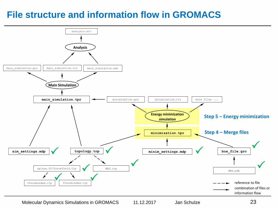
Step 4 – Merge files
Step 5 – Energy minimization
File structure and information flow in GROMACS
Molecular Dynamics Simulations in GROMACS 11.12.2017 Jan Schulze 23
topology.top
MEG.itpoplsaa.ff/forcefield.itp
ffnonbonded.itp ffnonbonded.itp reference to file
combination of files or
information flow
MEG.pdb
box_file.grominim_settings.mdp
minimization.tpr
Energy minimization
simulation
minimization.gro minimization.trr more files ...
Main Simulation
main_simulation.gro main_simulation.trr main_simulation.edr
main_simulation.tpr
sim_settings.mdp
Analysis
analysis.xtc
P
P
P
P
P
PP
P P
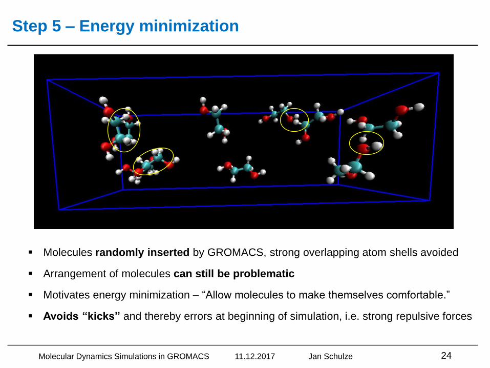
Step 5 – Energy minimization
Molecular Dynamics Simulations in GROMACS 11.12.2017 Jan Schulze 24
▪ Molecules randomly inserted by GROMACS, strong overlapping atom shells avoided
▪ Arrangement of molecules can still be problematic
▪ Motivates energy minimization – “Allow molecules to make themselves comfortable.”
▪ Avoids “kicks” and thereby errors at beginning of simulation, i.e. strong repulsive forces
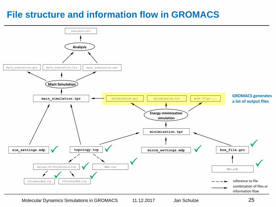
GROMACS generates a lot of output files
File structure and information flow in GROMACS
Molecular Dynamics Simulations in GROMACS 11.12.2017 Jan Schulze 25
topology.top
MEG.itpoplsaa.ff/forcefield.itp
ffnonbonded.itp ffnonbonded.itp reference to file
combination of files or
information flow
MEG.pdb
box_file.grominim_settings.mdp
minimization.tpr
Energy minimization
simulation
minimization.gro minimization.trr more files ...
Main Simulation
main_simulation.gro main_simulation.trr main_simulation.edr
main_simulation.tpr
sim_settings.mdp
Analysis
analysis.xtc
P
P
P
P
P
PP
P P
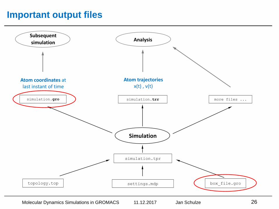
Important output files
Molecular Dynamics Simulations in GROMACS 11.12.2017 Jan Schulze 26
topology.top box_file.grosettings.mdp
simulation.tpr
Simulation
simulation.gro simulation.trr more files ...
Atom coordinates at last instant of time
Atom trajectoriesx(t) , v(t)
Subsequent
simulationAnalysis
File structure and information flow in GROMACS
Molecular Dynamics Simulations in GROMACS 11.12.2017 Jan Schulze 27
topology.top
MEG.itpoplsaa.ff/forcefield.itp
ffnonbonded.itp ffnonbonded.itp reference to file
combination of files or
information flow
MEG.pdb
box_file.grominim_settings.mdp
minimization.tpr
Energy minimization
simulation
minimization.gro minimization.trr more files ...
Main simulation
main_simulation.gro main_simulation.trr more files ...
main_simulation.tpr
sim_settings.mdp
Analysis
analysis.xtc
P
P
P
P
P
PP
P P
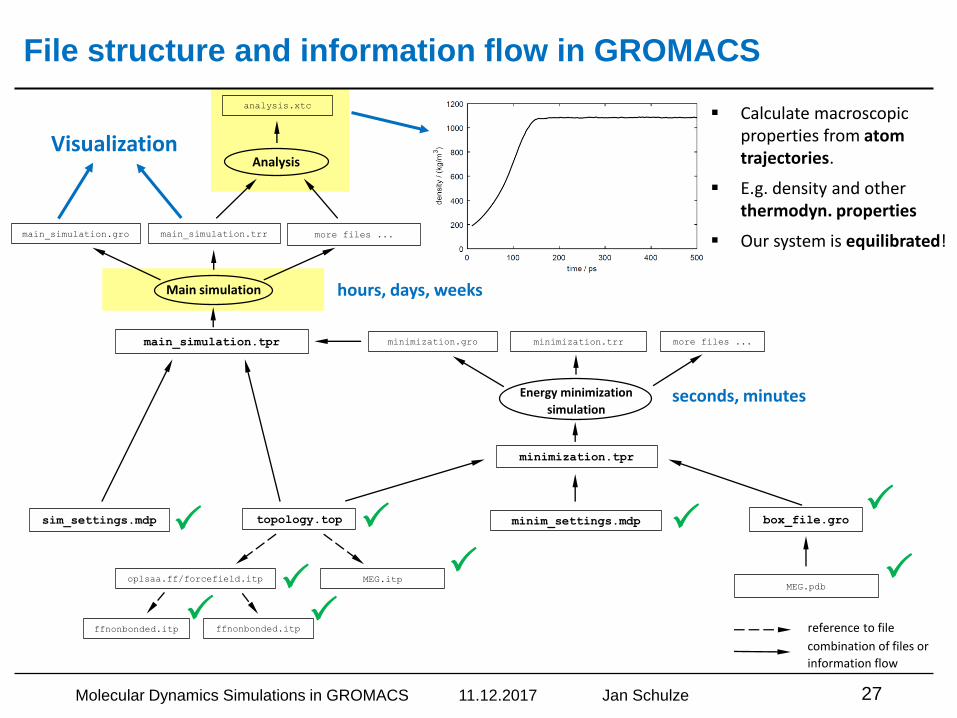
▪ Calculate macroscopic properties from atom trajectories.
▪ E.g. density and other thermodyn. properties
▪ Our system is equilibrated!
seconds, minutes
hours, days, weeks
Visualization
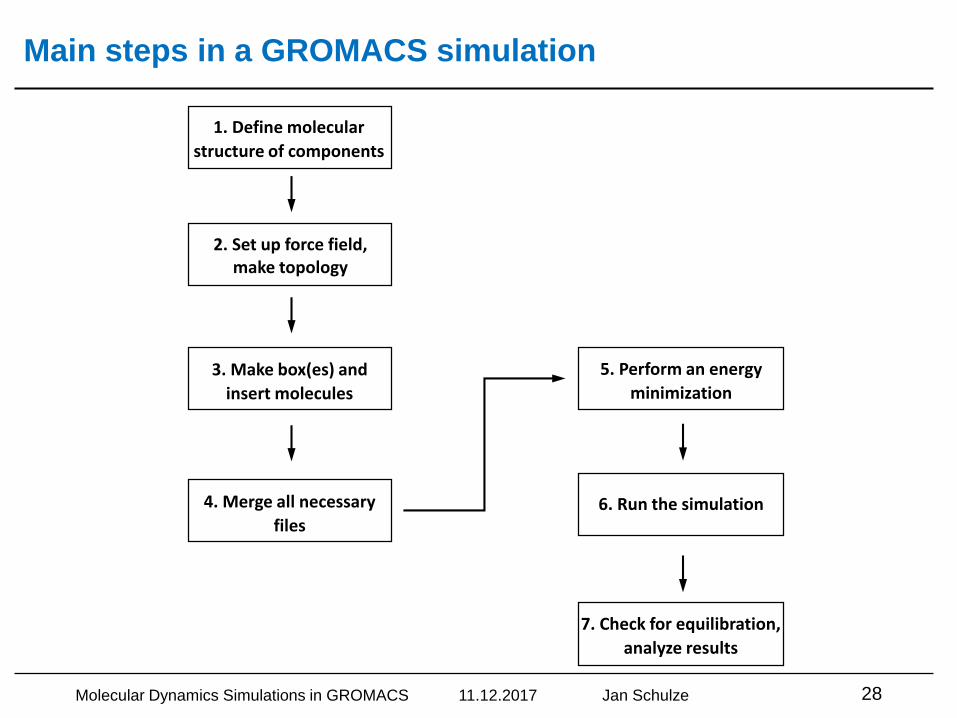
Main steps in a GROMACS simulation
Molecular Dynamics Simulations in GROMACS 11.12.2017 Jan Schulze 28
6. Run the simulation
7. Check for equilibration,
analyze results
1. Define molecular
structure of components
2. Set up force field,make topology
3. Make box(es) and
insert molecules
4. Merge all necessary
files
5. Perform an energy
minimization
End
Thanks for your attention!
Questions?
Molecular Dynamics Simulations in GROMACS 11.12.2017 Jan Schulze 29
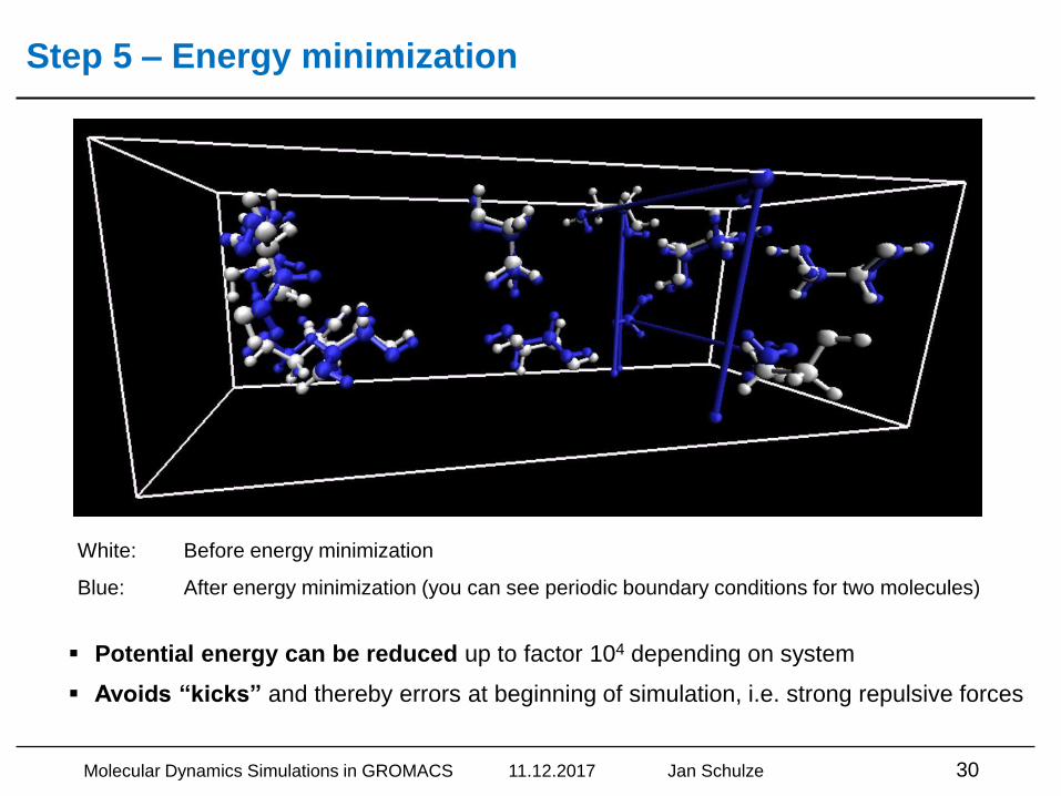
Step 5 – Energy minimization
White: Before energy minimization
Blue: After energy minimization (you can see periodic boundary conditions for two molecules)
Molecular Dynamics Simulations in GROMACS 11.12.2017 Jan Schulze 30
▪ Potential energy can be reduced up to factor 104 depending on system
▪ Avoids “kicks” and thereby errors at beginning of simulation, i.e. strong repulsive forces
Thermostat: Berendsen coupling
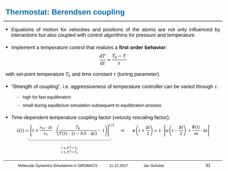
▪ Equations of motion for velocities and positions of the atoms are not only influenced byinteractions but also coupled with control algorithms for pressure and temperature.
▪ Implement a temperature control that realizes a first order behavior:
𝑑𝑇
𝑑𝑡=𝑇0 − 𝑇
𝜏
with set-point temperature 𝑇0 and time constant 𝜏 (tuning parameter).
▪ “Strength of coupling”, i.e. aggressiveness of temperature controller can be varied through 𝜏.
high for fast equilibration
small during equilibrium simulation subsequent to equilibration process
▪ Time-dependent temperature coupling factor (velocity rescaling factor):
𝜆 𝑡 = 1 +𝑛𝑇𝐶 ⋅ Δ𝑡
𝜏𝑇⋅
𝑇0𝑇 𝑡 ⋅ 𝑡 − 0.5 ⋅ Δ𝑡
− 1
1/2
⇒ 𝒗 𝑡 +Δ𝑡
2= 𝜆 ⋅ 𝒗 𝑡 −
Δ𝑡
2+𝐅 t
m⋅ Δ𝑡
Molecular Dynamics Simulations in GROMACS 11.12.2017 Jan Schulze 31
> 1, if T < T0
< 1, if T > T0


![FEFLOW Hydromechanical Coupling Plugin...5 2.2 Parametricmodel for single fractures The effective-stressmodel for fractured regions after Preisig et al. [2012] applied to sets of discrete](https://img.pdfslide.us/doc/110x75/6135ea0c0ad5d2067647ae5c/feflow-hydromechanical-coupling-plugin-5-22-parametricmodel-for-single-fractures.jpg)


![TensorFlow - NTNUfolk.ntnu.no/preisig/HAP_Specials... · using more complicated neural networks, automatic generation of email responses can be made [2]. Google search has also started](https://img.pdfslide.us/doc/110x75/5ec471647de7b60a1b6d7896/tensorflow-using-more-complicated-neural-networks-automatic-generation-of-email.jpg)