Embed Size (px)
Citation preview
MOLECULAR DYNAMICS SIMULATION OF A NANOSCALE DEVICE FOR FAST
SEQUENCING OF DNA
By
Christina M. Payne
Dissertation
Submitted to the Faculty of the
Graduate School of Vanderbilt University
in partial fulfillment of the requirements
for the degree of
DOCTOR OF PHILOSOPHY
in
Chemical Engineering
December 2007
Nashville, Tennessee
Approved:
Peter T. Cummings
M. Douglas LeVan
G. Kane Jennings
Clare McCabe
Jens Meiler

ii
To my mother, Janice, for her unconditional love and support
and
To my friends, for their endless encouragement

iii
ACKNOWLEDGEMENTS
This work has been made possible through the financial support of the
Department of Energy Computational Science Graduate Fellowship under grant number
DE-FG02-97ER25308. I am extraordinarily grateful to have been a part of such an
incredibly gifted and unique group of individuals comprising the CSGF fellows.
Additional financial support for related research performed at Oak Ridge National
Laboratory was provided by the National Institutes of Health under grant number
1R21HG003578-01.
I am grateful for all of the support and guidance I have received during my
research from my advisor, Professor Peter T. Cummings. I would also like to thank the
members of my Dissertation Committee for offering valuable insight and suggestions as
well as Dr. Paul Crozier at Sandia National Laboratory for his exceptional mentorship
and assistance.
I would like to thank Dr. James W. Lee of the Chemical Sciences Division of Oak
Ridge National Laboratory for introducing the proposed nanoscale sequencing device and
for helpful discussions. Dr. Lukas Vlcek is due special thanks for his help implementing
electrode charge dynamics in LAMMPS.
Finally, I would like to thank my family and friends for their unconditional love
and support in all my endeavors. Without them, I would not be the woman I am today.
iv
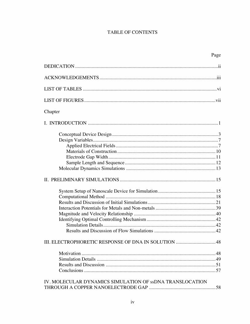
TABLE OF CONTENTS
Page
DEDICATION................................................................................................................ii
ACKNOWLEDGEMENTS............................................................................................iii
LIST OF TABLES .........................................................................................................vi
LIST OF FIGURES.......................................................................................................vii
Chapter
I. INTRODUCTION ......................................................................................................1
Conceptual Device Design...................................................................................3Design Variables..................................................................................................7
Applied Electrical Fields ................................................................................7Materials of Construction............................................................................. 10Electrode Gap Width.................................................................................... 11Sample Length and Sequence....................................................................... 12
Molecular Dynamics Simulations ...................................................................... 13
II. PRELIMINARY SIMULATIONS........................................................................... 15
System Setup of Nanoscale Device for Simulation............................................. 15Computational Method ...................................................................................... 18Results and Discussion of Initial Simulations..................................................... 21Interaction Potentials for Metals and Non-metals ............................................... 39Magnitude and Velocity Relationship ................................................................ 40Identifying Optimal Controlling Mechanism...................................................... 42
Simulation Details........................................................................................ 42Results and Discussion of Flow Simulations ................................................ 42
III. ELECTROPHORETIC RESPONSE OF DNA IN SOLUTION ............................... 48
Motivation ......................................................................................................... 48Simulation Details ............................................................................................. 49Results and Discussion ...................................................................................... 51Conclusions ....................................................................................................... 57
IV. MOLECULAR DYNAMICS SIMULATION OF ssDNA TRANSLOCATIONTHROUGH A COPPER NANOELECTRODE GAP .................................................... 58
v
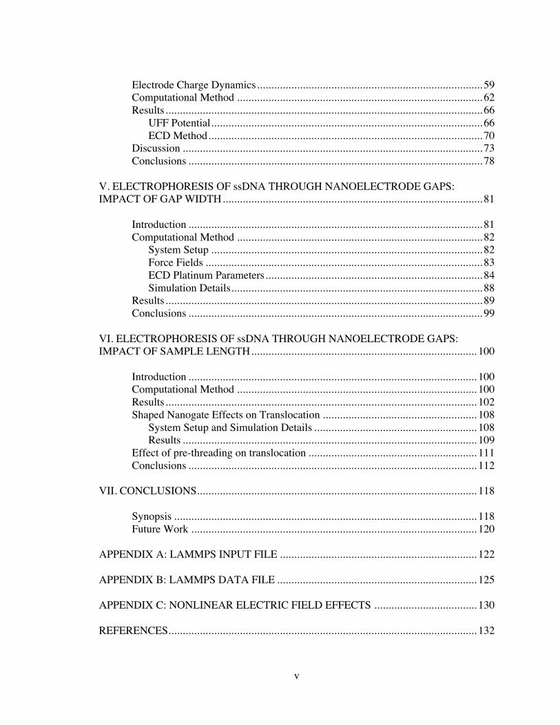
Electrode Charge Dynamics............................................................................... 59Computational Method ...................................................................................... 62Results............................................................................................................... 66
UFF Potential............................................................................................... 66ECD Method................................................................................................ 70
Discussion ......................................................................................................... 73Conclusions ....................................................................................................... 78
V. ELECTROPHORESIS OF ssDNA THROUGH NANOELECTRODE GAPS:IMPACT OF GAP WIDTH........................................................................................... 81
Introduction ....................................................................................................... 81Computational Method ...................................................................................... 82
System Setup ............................................................................................... 82Force Fields ................................................................................................. 83ECD Platinum Parameters............................................................................ 84Simulation Details........................................................................................ 88
Results............................................................................................................... 89Conclusions ....................................................................................................... 99
VI. ELECTROPHORESIS OF ssDNA THROUGH NANOELECTRODE GAPS:IMPACT OF SAMPLE LENGTH............................................................................... 100
Introduction ..................................................................................................... 100Computational Method .................................................................................... 100Results............................................................................................................. 102Shaped Nanogate Effects on Translocation ...................................................... 108
System Setup and Simulation Details ......................................................... 108Results ....................................................................................................... 109
Effect of pre-threading on translocation ........................................................... 111Conclusions ..................................................................................................... 112
VII. CONCLUSIONS.................................................................................................. 118
Synopsis .......................................................................................................... 118Future Work .................................................................................................... 120
APPENDIX A: LAMMPS INPUT FILE ..................................................................... 122
APPENDIX B: LAMMPS DATA FILE ...................................................................... 125
APPENDIX C: NONLINEAR ELECTRIC FIELD EFFECTS .................................... 130
REFERENCES............................................................................................................ 132
vi
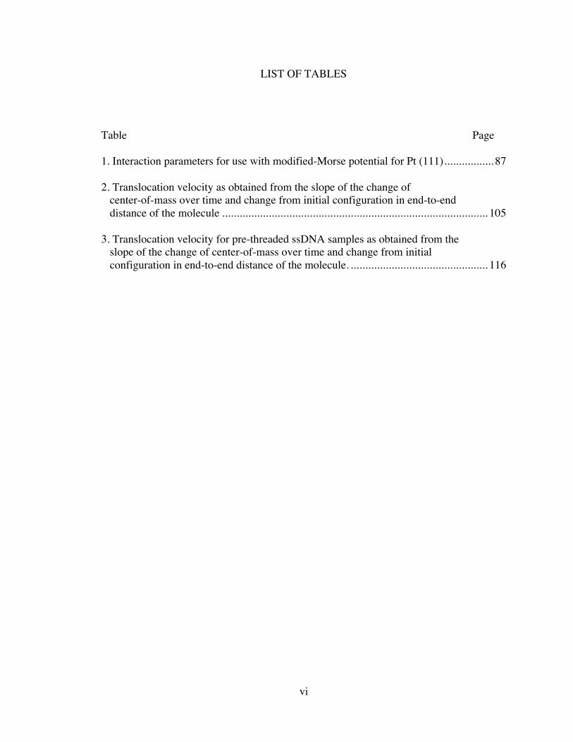
LIST OF TABLES
Table Page
1. Interaction parameters for use with modified-Morse potential for Pt (111)................. 87
2. Translocation velocity as obtained from the slope of the change ofcenter-of-mass over time and change from initial configuration in end-to-enddistance of the molecule ........................................................................................... 105
3. Translocation velocity for pre-threaded ssDNA samples as obtained from theslope of the change of center-of-mass over time and change from initialconfiguration in end-to-end distance of the molecule. ............................................... 116
vii
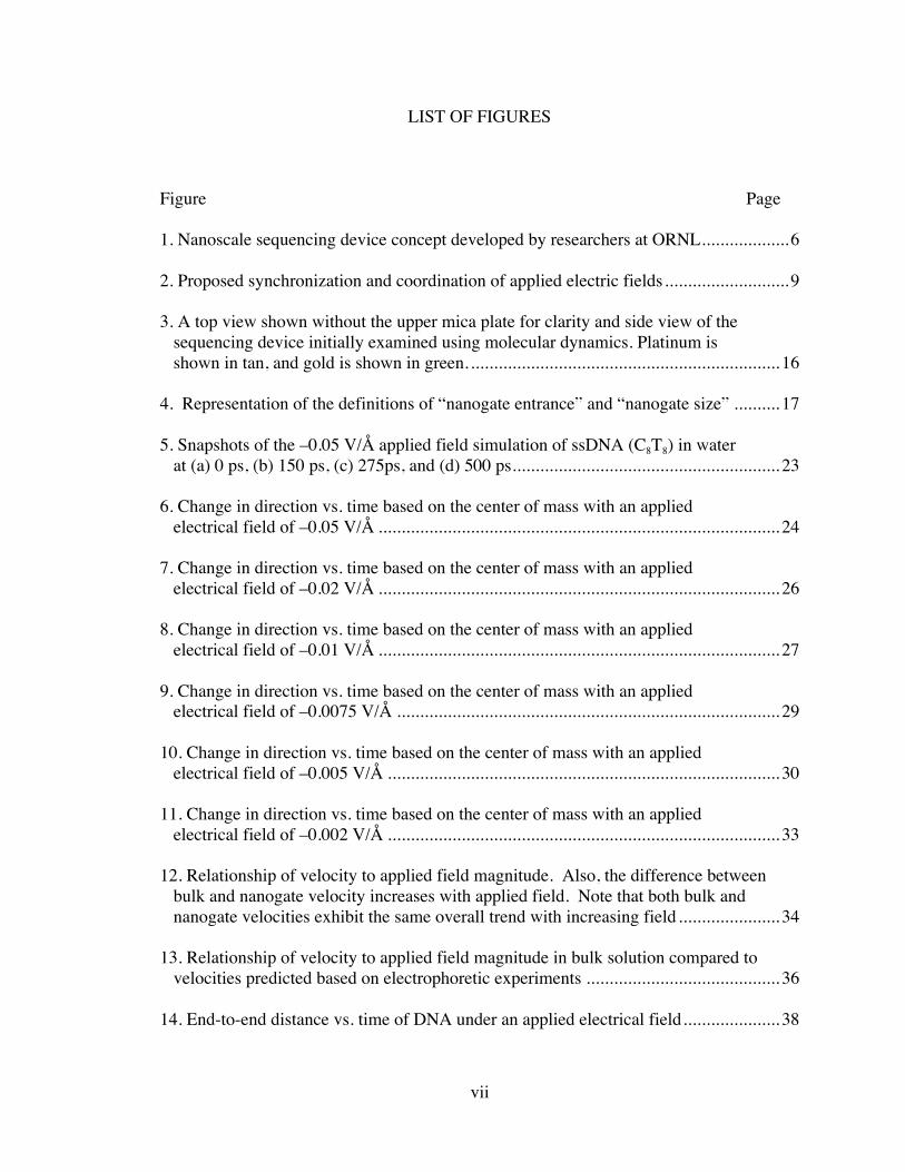
LIST OF FIGURES
Figure Page
1. Nanoscale sequencing device concept developed by researchers at ORNL...................6
2. Proposed synchronization and coordination of applied electric fields...........................9
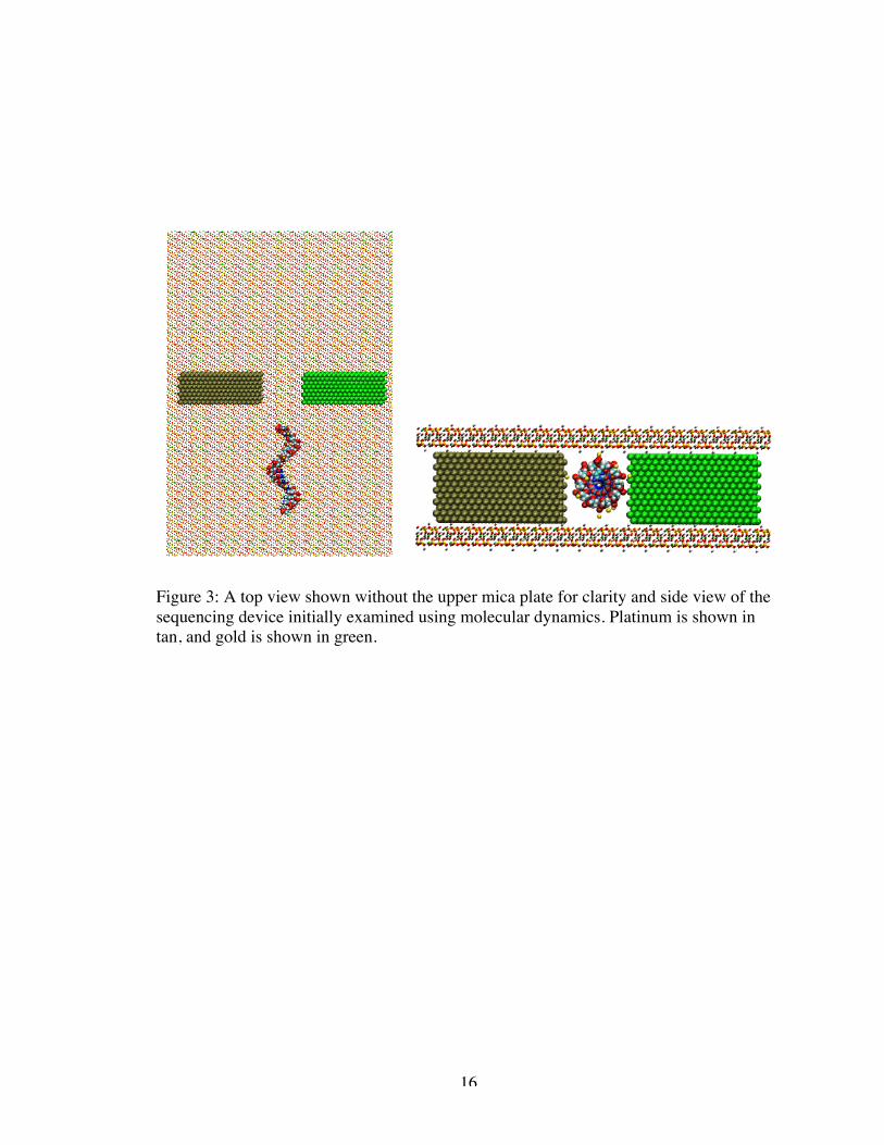
3. A top view shown without the upper mica plate for clarity and side view of thesequencing device initially examined using molecular dynamics. Platinum isshown in tan, and gold is shown in green. ................................................................... 16
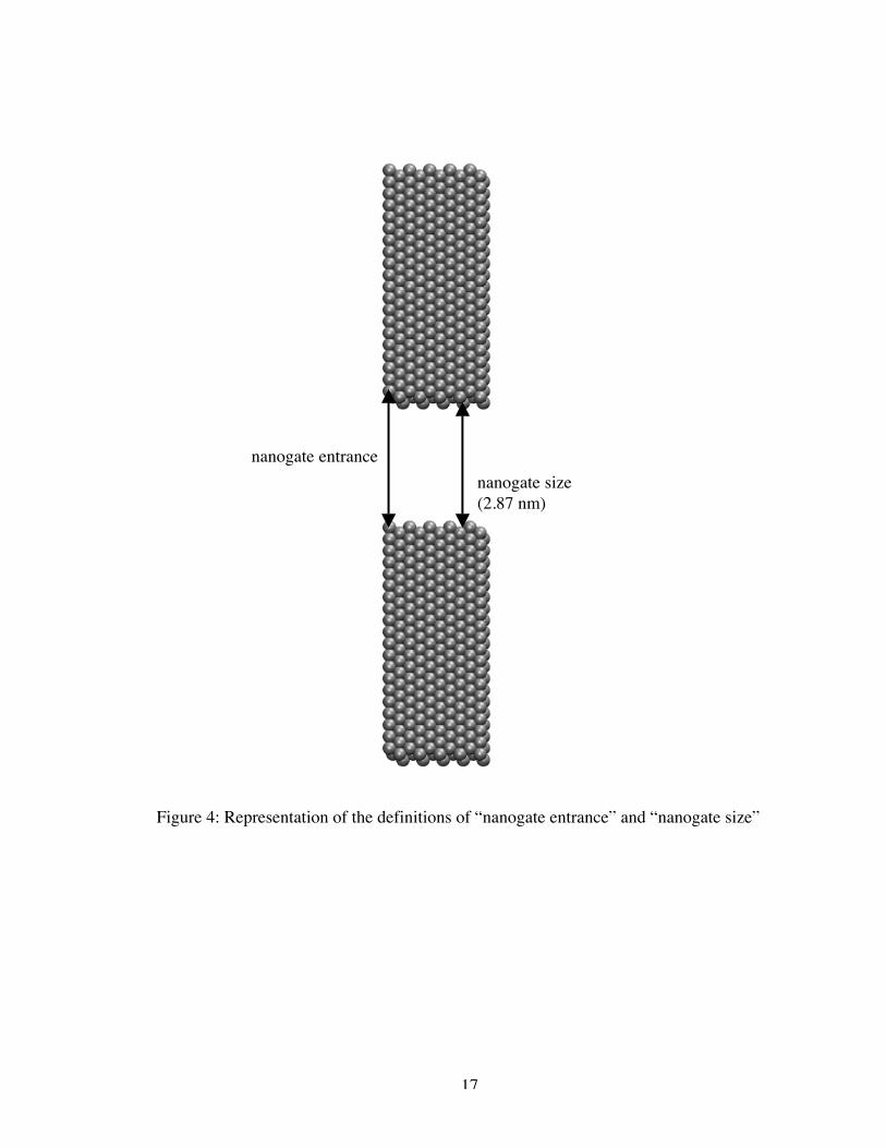
4. Representation of the definitions of “nanogate entrance” and “nanogate size” .......... 17
5. Snapshots of the –0.05 V/Å applied field simulation of ssDNA (C8T8) in waterat (a) 0 ps, (b) 150 ps, (c) 275ps, and (d) 500 ps.......................................................... 23
6. Change in direction vs. time based on the center of mass with an appliedelectrical field of –0.05 V/Å ....................................................................................... 24
7. Change in direction vs. time based on the center of mass with an appliedelectrical field of –0.02 V/Å ....................................................................................... 26
8. Change in direction vs. time based on the center of mass with an appliedelectrical field of –0.01 V/Å ....................................................................................... 27
9. Change in direction vs. time based on the center of mass with an appliedelectrical field of –0.0075 V/Å ................................................................................... 29
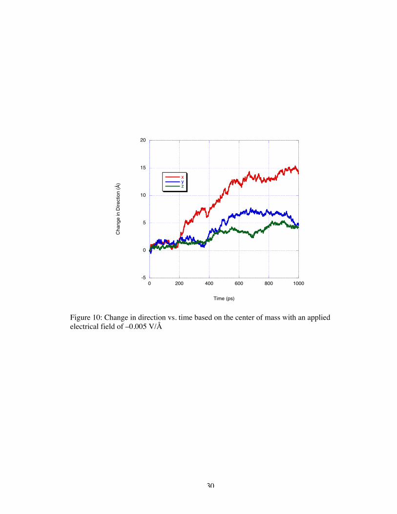
10. Change in direction vs. time based on the center of mass with an appliedelectrical field of –0.005 V/Å ..................................................................................... 30
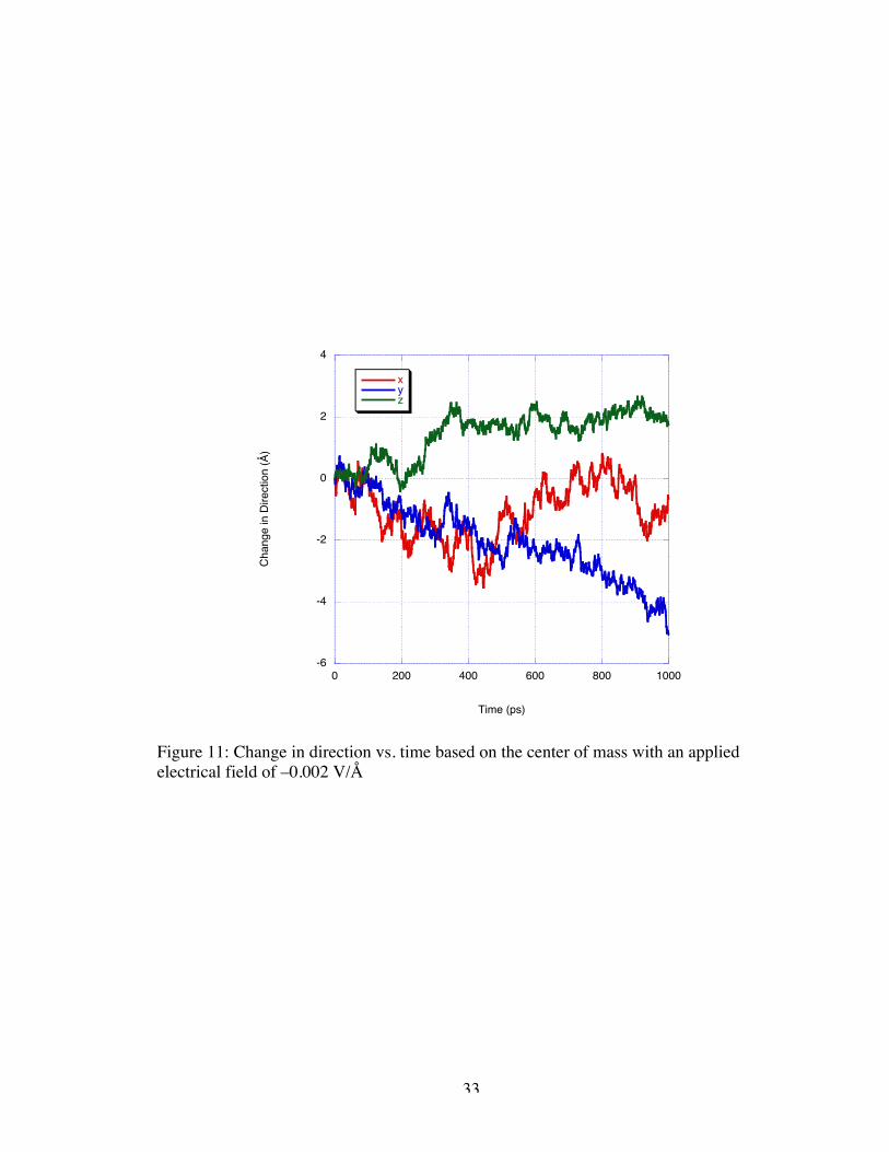
11. Change in direction vs. time based on the center of mass with an appliedelectrical field of –0.002 V/Å ..................................................................................... 33
12. Relationship of velocity to applied field magnitude. Also, the difference betweenbulk and nanogate velocity increases with applied field. Note that both bulk andnanogate velocities exhibit the same overall trend with increasing field ...................... 34
13. Relationship of velocity to applied field magnitude in bulk solution compared tovelocities predicted based on electrophoretic experiments .......................................... 36
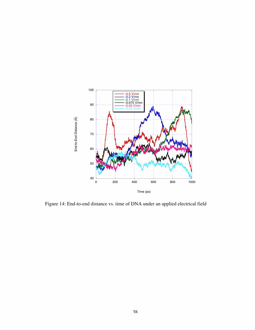
14. End-to-end distance vs. time of DNA under an applied electrical field..................... 38
viii
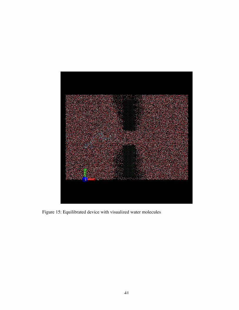
15. Equilibrated device with visualized water molecules................................................ 41
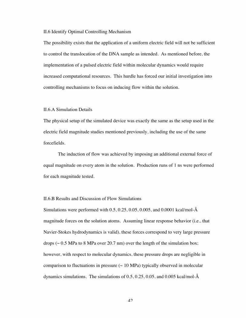
16. Snapshots of the 0.05 kcal/mol-Å magnitude force simulation of ssDNA (C8T8)in water at (a) 0 ps and (b) 1000 ps ............................................................................. 44
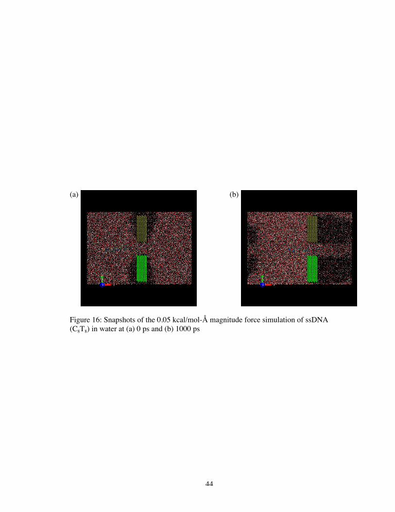
17. Change in direction vs. time based on the center of mass with an applied force of0.0001 kcal/mol-Å...................................................................................................... 46
18. End-to-end distance vs. time of DNA under an applied force of0.0001 kcal/mol-Å...................................................................................................... 47
19. Center of mass motion in the z-direction for the ssA5 molecule versus time forapplied fields 0.003, 0.03, 0.04, and 0.05 V/Å. The open triangles, circles,squares, and filled squares are not representative of data points but merely amethod of differentiating lines.................................................................................... 52
20. Center of mass motion in the z-direction for the dsA5 molecule versus time forapplied fields 0.003, 0.03, 0.04, and 0.05 V/Å. The open triangles, circles,squares, and filled squares are not representative of data points but merely amethod of differentiating lines.................................................................................... 53
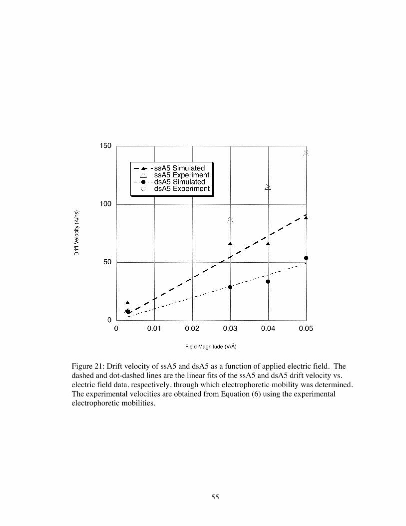
21. Drift velocity of ssA5 and dsA5 as a function of applied electric field. The dashedand dot-dashed lines are the linear fits of the ssA5 and dsA5 drift velocity vs. electricfield data, respectively, through which electrophoretic mobility was determined. Theexperimental velocities are obtained from Equation (6) using the experimentalelectrophoretic mobilities. .......................................................................................... 55
22. Change in position in x-direction vs. time based upon the center of mass resultingfrom the application of an external electric field (UFF potential simulations).Figure a shows the four lowest magnitude applied fields. Note that the origin ofeach curve is shifted upwards by 10Å for clarity. Figure b shows the four highestmagnitude applied fields............................................................................................. 68
23. Snapshot of the 0.01 V/Å simulation at 1 ns utilizing (a) UFF and (b) ECD............. 69
24. Change in position in x-direction vs. time based upon the center of mass resultingfrom the application of an external electric field (ECD potential simulations).Figure a shows the four lowest magnitude applied fields. Note that the origin ofeach curve is shifted upwards by 10Å for clarity. Figure b shows the four highestmagnitude applied fields............................................................................................. 72
25. Translocation velocity vs. electric field magnitude for UFF and ECDsimulation sets............................................................................................................ 74
ix
26. Density profile across the nanogate utilizing the UFF and ECD potential.Note that the distance between the peaks at each surface is approximately 2.5 nmfor the ECD method ................................................................................................... 79
27. (a) Density profile across mica surfaces utilizing the UFF and ECD potential.(b) Bulk area from which density profile in (a) was obtained is marked by thesquare in the upper left of the device picture............................................................... 80
28. Modified-Morse potential fit for Pt(111) ECD parameters. (a) Energy as watermolecule is moved vertically from the surface and (b) energy as water moleculeis tilted from the surface holding the oxygen atom 2.43 Å above the platinumtop-site. ...................................................................................................................... 86
29. Change in position in x-direction vs. time based on the center of mass resultingfrom the application of an external electric field ......................................................... 90
30. Snapshot of 1.75 nm gate width simulation after 1 ns production run (water notshown for clarity). ...................................................................................................... 92
31. Snapshot of 3.25 nm gate width simulation after 1 ns production run (water notshown for clarity). ...................................................................................................... 94
32. End-to-End distance vs. time measured between the carbon atoms of the first andsixteenth residues ....................................................................................................... 95
33. Snapshots of the 0.02 V/Å applied field simulation of ssDNA (C8T8) in water throughthe 3.25 nm gate at (a) 0 ps, (b) 250 ps, (c) 500ps, and (d) 1000 ps. Red indicatespositive charge, and blue indicates negative charge. White is the mid-point of thecharge gradient. .......................................................................................................... 98
34. Change in position in x-direction vs. time based on the center of mass resultingfrom the application of an external electric field ....................................................... 104
35. Snapshots of the –0.02 V/Å applied field simulation of 4CTAG in water througha 3.0 nm gate at (a) 0 ps, (b) 250 ps, (c) 500ps, and (d) 1000 ps ................................ 106
36. Snapshots of the –0.02 V/Å applied field simulation of 4CTAG in water throughthe shaped nanogate at (a) 0 ps, (b) 250 ps, (c) 500ps, and (d) 1000 ps...................... 110
37. Snapshots of the –0.02 V/Å applied field simulation of 4CTAG in waterpre-threaded 1 nm inside the nanogate (a) unequilibrated and (b) at 1000 ps............. 114
38. Change in position in x-direction vs. time of the pre-threaded ssDNA samplesbased upon the center of mass resulting from the application of an external electricfield.......................................................................................................................... 115

x
39. Summary of translocation velocities for different length ssDNA segments.The results shown consist of the simulations exhibiting translocation in Table 2(CTAG, 2CTAG, 6CTAG, 12CTAG) and the results reported in Table 3 in whichthe molecules were placed 1 nm inside the nanogap. The average translocationvelocity is 43±8 A/ns. If the outlying result (4CTAG) is removed, the averagetranslocation velocity is 46±4 A/ns. .......................................................................... 117
1
CHAPTER I
INTRODUCTION
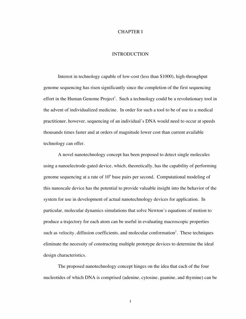
Interest in technology capable of low-cost (less than $1000), high-throughput
genome sequencing has risen significantly since the completion of the first sequencing
effort in the Human Genome Project1. Such a technology could be a revolutionary tool in
the advent of individualized medicine. In order for such a tool to be of use to a medical
practitioner, however, sequencing of an individual’s DNA would need to occur at speeds
thousands times faster and at orders of magnitude lower cost than current available
technology can offer.
A novel nanotechnology concept has been proposed to detect single molecules
using a nanoelectrode-gated device, which, theoretically, has the capability of performing
genome sequencing at a rate of 106 base pairs per second. Computational modeling of
this nanoscale device has the potential to provide valuable insight into the behavior of the
system for use in development of actual nanotechnology devices for application. In
particular, molecular dynamics simulations that solve Newton’s equations of motion to
produce a trajectory for each atom can be useful in evaluating macroscopic properties
such as velocity, diffusion coefficients, and molecular conformation2. These techniques
eliminate the necessity of constructing multiple prototype devices to determine the ideal
design characteristics.
The proposed nanotechnology concept hinges on the idea that each of the four
nucleotides of which DNA is comprised (adenine, cytosine, guanine, and thymine) can be
2
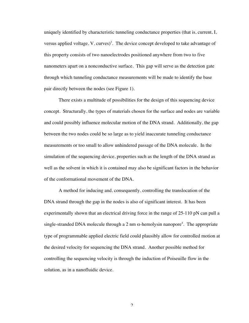
uniquely identified by characteristic tunneling conductance properties (that is, current, I,
versus applied voltage, V, curves)3. The device concept developed to take advantage of
this property consists of two nanoelectrodes positioned anywhere from two to five
nanometers apart on a nonconductive surface. This gap will serve as the detection gate
through which tunneling conductance measurements will be made to identify the base
pair directly between the nodes (see Figure 1).
There exists a multitude of possibilities for the design of this sequencing device
concept. Structurally, the types of materials chosen for the surface and nodes are variable
and could possibly influence molecular motion of the DNA strand. Additionally, the gap
between the two nodes could be so large as to yield inaccurate tunneling conductance
measurements or too small to allow unhindered passage of the DNA molecule. In the
simulation of the sequencing device, properties such as the length of the DNA strand as
well as the solvent in which it is contained may also be significant factors in the behavior
of the conformational movement of the DNA.
A method for inducing and, consequently, controlling the translocation of the
DNA strand through the gap in the nodes is also of significant interest. It has been
experimentally shown that an electrical driving force in the range of 25-110 pN can pull a
single-stranded DNA molecule through a 2 nm α-hemolysin nanopore4. The appropriate
type of programmable applied electric field could plausibly allow for controlled motion at
the desired velocity for sequencing the DNA strand. Another possible method for
controlling the sequencing velocity is through the induction of Poiseuille flow in the
solution, as in a nanofluidic device.
3
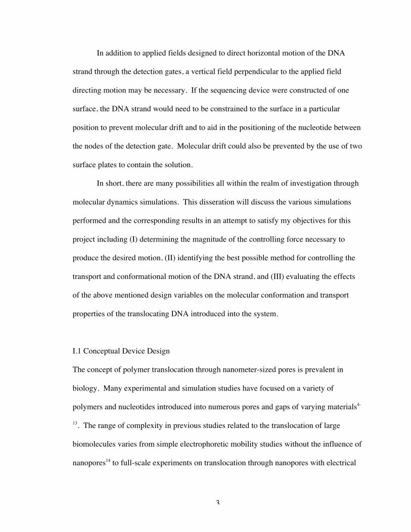
In addition to applied fields designed to direct horizontal motion of the DNA
strand through the detection gates, a vertical field perpendicular to the applied field
directing motion may be necessary. If the sequencing device were constructed of one
surface, the DNA strand would need to be constrained to the surface in a particular
position to prevent molecular drift and to aid in the positioning of the nucleotide between
the nodes of the detection gate. Molecular drift could also be prevented by the use of two
surface plates to contain the solution.
In short, there are many possibilities all within the realm of investigation through
molecular dynamics simulations. This disseration will discuss the various simulations
performed and the corresponding results in an attempt to satisfy my objectives for this
project including (I) determining the magnitude of the controlling force necessary to
produce the desired motion, (II) identifying the best possible method for controlling the
transport and conformational motion of the DNA strand, and (III) evaluating the effects
of the above mentioned design variables on the molecular conformation and transport
properties of the translocating DNA introduced into the system.
I.1 Conceptual Device Design
The concept of polymer translocation through nanometer-sized pores is prevalent in
biology. Many experimental and simulation studies have focused on a variety of
polymers and nucleotides introduced into numerous pores and gaps of varying materials4-
13. The range of complexity in previous studies related to the translocation of large
biomolecules varies from simple electrophoretic mobility studies without the influence of
nanopores14 to full-scale experiments on translocation through nanopores with electrical
4
driving forces4-9. For the most part, the research relevant to the aims of this project has
occurred within the past ten years, and only recently has research on similarly structured
nanoscale systems become the focus of genomic sequencing efforts.
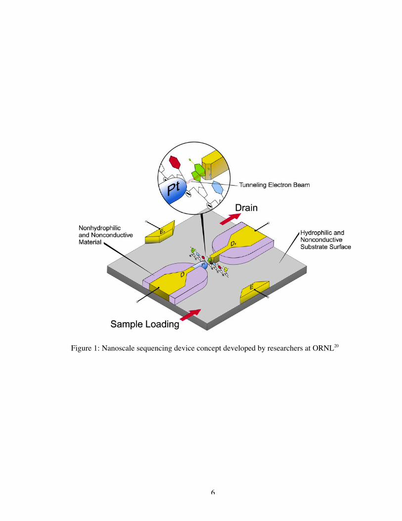
In conjunction with the experimental development of this project at Oak Ridge
National Laboratories (ORNL), a basic device concept has been developed as shown in
Figure 1. This conceptual device design is based on the precision electrolytic
nanofabrication technique patented by Lee and Greenbaum at ORNL15, 16 by which
metallic atoms can be precisely deposited on the nonconductive and hydrophilic surface
with an extremely small distance (1-10 nm) between the nanoelectrode tips. A pair of
macroelectrodes will provide the electrophoretic field required to induce translocation of
the DNA strand through the nanogap in the detection electrodes. The DNA sample
molecules will be loaded into the device using micropipetting and/or microfluidic
techniques.
The sequencing of the individual nucleotides as the DNA sample travels through
the electrodes will be accomplished through the application of a tunneling electron beam
across the metal electrodes. In theory, each of the four nucleotides has a unique
corresponding conductance measurement. Measurement of this conductance will
ultimately yield the sample sequence. In practice, this characteristic has yet to be proven
either theoretically or in experiment. Additionally, theoretical studies of nucleotide
conductance have been inconclusive. The most positive results indicating conductance
sequencing techniques are a possibility have been published by Lagerqvist, et al.17, 18.
They concluded through a combination of quantum-mechanical calculations of current
and molecular dynamics simulations of DNA translocation that, in the absence of
5
structural fluctions, ions, and water, it is very likely DNA can be sequenced through a
nanopore should dynamics be controllable. A second study of the feasibility of
transversal DNA conductance measurement was reported by Zhang, et al.19. This study
used first-principles calculation to determine transverse conductance across DNA
fragments between gold nanoelectrodes. The conclusion presented here is that the
conductance measurements of the four nucleotides differ only as a result of geometrical
size (i.e. the space remaining between the sample and the electrodes). As this would be
extraordinarily difficult to control in an on-the-fly sequencing device, they suggest this
method of sequencing is not viable as a matter of convenience. The drawback to both of
the theoretical studies of tunneling conductance measurements is their highly idealized
simulation setups. Both examine DNA in the absence of realistic environments, such as
the presence of solvent and counterions. Additionally, the first-principles study presented
by Zhang does not represent the behavior of DNA at finite temperatures. Lacking a
decisive conclusion on the feasibility of tunneling conductance sequencing techniques,
we have continued the molecular dynamics study of transport behavior of such a device
as presented here.
6
Figure 1: Nanoscale sequencing device concept developed by researchers at ORNL20
7
I.2 Design Variables
I.2.A Applied Electrical Fields
As mentioned before, there exist several variables in the conceptual design that may have
significant effects on the functional operation of the nanoscale device. The variable at
the forefront of this investigation is the use of an electrophoretic field to control
translocation of the DNA strand. The importance of this applied electric field lies in the
necessity of providing sufficient residence time between the nanogap and maintaining
vertical stability of the molecule. Without an external driving force, the DNA strand
likely will not move between the nanogap or maintain a velocity suitable for the purpose
of base pair detection.
DNA is a negatively charged molecule having a charge of –1 per base pair.
Positively charged counterions exist in solution around the DNA molecule to maintain a
charge-neutral system and the proper conformation of the molecule. When an electric
field is applied to the DNA in solution, the entire strand should move toward the anode
while the counterions will move in the opposite direction. Many experimental studies
have been performed using a voltage bias to induce movement of DNA in solution. In
particular, Meller et al.4 used an electrophoretic driving force to force single-stranded
DNA through a 2 nm diameter α-hemolysin nanopore.
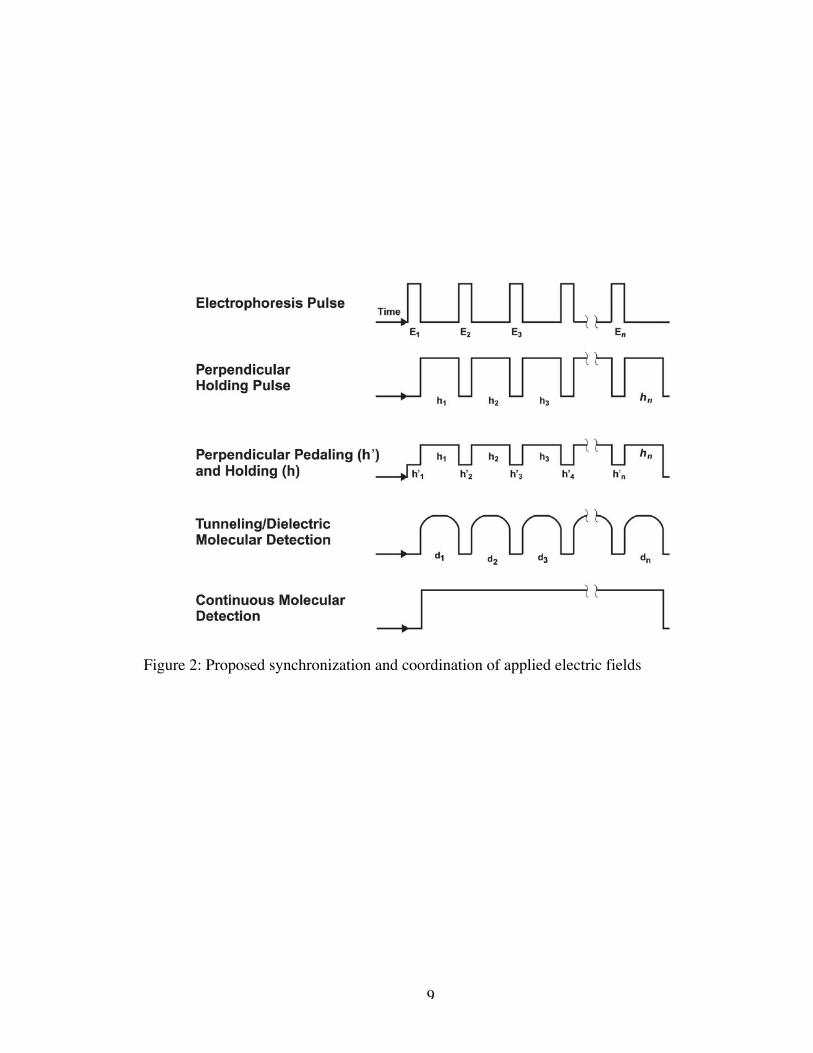
Controlling the transduction of the DNA strand may not be as simple as the
application of a uniform electrical field, however. The required detection period may
necessitate the use of an electrophoretic pulse as shown in Figure 2. While this is an
experimentally feasible solution to the problem of controlling motion, implementation of
8
a pulsing field in a molecular dynamics simulation presents a problem due to the
timescale relation to reality. Experimental pulsing of a field includes a ramp-up period of
approximately 10 ns and, likewise, a ramp-down period of 10 ns in addition to the pulse
period. Thus, modeling a realistic electrical pulse would require simulation times of at
least 20 ns. These timescales are not completely unattainable; however, the
computational cost of such simulations strongly suggests studying a uniform electric field
initially. Investigation of the electrical driving force is primarily for determining an
appropriate magnitude.
In the experimental design, there is also a need for a perpendicular holding field
to properly align the DNA strand between the detection electrodes and retain it on the
surface of the sample plate. The negatively charged phosphate groups along the
backbone of the DNA will serve to align the DNA strand with the application of a
perpendicular field as seen in the inset of Figure 1. An additional applied field across the
detection nodes is necessary to perform the tunneling conductance measurements by
which nucleotide sequence will be determined.
9
Figure 2: Proposed synchronization and coordination of applied electric fields
10
I.2.B Materials of Construction
The material chosen for the prototype design of the nanoscale-sequencing device has
been determined to suit both experimental and simulation needs. The surface of the
sample plates must be constructed out of a nonconductive and hydrophilic material. The
sample plates must be nonconductive as to not interfere with the tunneling conductance
measurements and hydrophilic so that the solvent will wet the surface and not create any
adverse interactions that may affect the movement of the DNA strand. The device must
also be designed to minimize leakage current to potentially improve the detection
sensitivity. Initially, the surface material of interest was silicon dioxide; however, this
material proved to be too rough at 1 nm, approximately the size of the molecules of
interest in simulations. A paper by Leng and Cummings21 presents results of the
molecular dynamics simulations of water confined between two mica surfaces indicating
that water confined between mica surfaces of the separation distance needed for the
nanoscale device (~ 3 nm) does not exhibit abnormal fluidic behavior. Thus, mica
surfaces have been used in simulations.
The electrodes must be conductive to achieve the intended purpose as tunneling
current detection nodes. The electrolytic nanofabrication technique mentioned previously
has been developed to precisely fabricate (approximately 100 atoms per step) a gap as
narrow as 1 to 10 nm by deposition or depletion of metal. Consequently, metal nodes are
ideal for the purpose of molecular detection nodes in the proposed sequencing device.
Currently, the experimental plans call for platinum and/or gold nodes though, as will be
shown, we have also made use of copper electrodes in many of our simulations. Again,
the issue of current leakage is a factor in the sensitivity of the nanoelectrode-gated
11
detection system. It is only possible to use charge transport through the molecule as a
means of detection when the leakage current is less than the tunneling current. This can
be controlled by the addition of insulating shields around the sides of the detection
electrodes, which should be constructed of a hydrophilic, nonconductive substrate such as
silicon nitride (SiN). This is not reflected directly in simulations, however, because of
the discrepancy in scale.
A final element in construction of the sequencing device is the choice of solvent
in which the DNA sample is contained. The device has been developed under the
assumption that the solvent will be water. For now, the simulations are being carried out
in an aqueous environment, but it may be necessary to incorporate a more viscous solvent
to achieve the desired control over the motion of the DNA sample.
I.2.C Electrode Gap Width
Experimentally, the gap distance between the electrodes can be fabricated as small as 1
nm creating a natural lower bound to the gap distance. Additionally, the electrodes must
be within a few nanometers to observe a large tunneling current for detection purposes,
resulting in an upper bound. The diameter of the DNA helix, 2 nm22, gives a good
estimate as to the actual value to choose.
While some stretching of bonds during translocation is acceptable, significant
denaturation of the strand may adversely affect the detection process, so the gap must not
be so small as to prevent reasonable conformational motion. In the paper by Heng, el.
al.5, the electrophoretically-driven DNA strand forced through a 1.2 nm pore in a Si3N4
membrane exhibited rupture of hydrogen bonds connecting three terminal base pairs.
12
However, the experimental studies performed by Meller, et al.4 utilized a 2 nm diameter
α-hemolysin pore in effectively allowing passage of a single-stranded DNA sample with
clear evidence of elongation but no bond breakage.
Furthermore, large gap distances allow for folding of the sample as it passes
through the detection gate. Studies by Storm, et al.7 indicate that a pore diameter of 10
nm allows for the passage of DNA in a folded conformation. For proper nucleotide
detection, the DNA must pass through the gap a single base pair at a time. Thus, the gap
must be much smaller than 10 nm, most likely, closer to the lower distance constraint.
I.2.D Sample Length and Sequence
In 2001, Meller, et al.4 performed experiments in which single-stranded DNA polymers
were driven through a single α-hemolysin pore (2 nm in diameter and 5.2 nm depth) by
an applied electrical field with the purpose of measuring current blockage across the
length of the pore as the DNA strand is in residence as well as time distribution as it is
related to length of the strand. Using the current blockade measurement to estimate
residence time, and thus velocity, the authors conclude that strands longer than the length
of the pore travel at a constant velocity while the velocity of shorter strands increases
with decreasing length.
Storm, et al.7 experimentally investigated the relationship of translocation time
and length of double-stranded DNA electrophoretically driven through a 10 nm diameter
silicon oxide pore of approximately 20 nm in depth. They observed a power-law scaling
of translocation time with length. Though this likely will not hold true for smaller
diameter pores, these studies indicate the importance of sample length with regard to pore
13
length. The majority of the simulations presented here use a single-stranded DNA
sample of 16 nucleotides, which is approximately 5.5 nm in length. We also present a
sample length simulation study in which the largest sample molecule is 48 nucleotides
long. We are limited in sample length by simulation device design. The length of the
pore, or gate, of the current design in this dissertation is approximately 2 nm. Hence, in
our cased, the DNA length is longer than the pore length. On the basis of the Meller, et
al.4 experiment, we should expect to see constant translocation speed through the “pore”
created by the nanoelectrodes.
I.3 Molecular Dynamics Simulation
In this work, the simulations being performed are known as classical molecular dynamics
simulations. This method of simulation determines atomic trajectory by using an
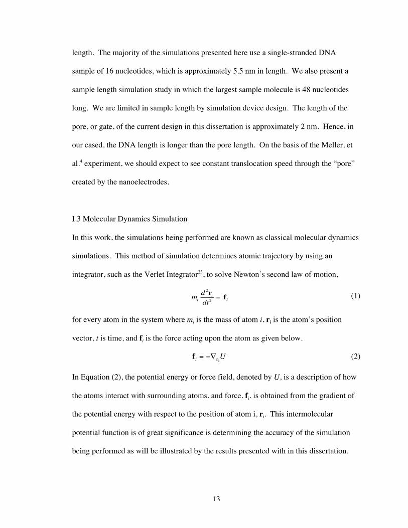
integrator, such as the Verlet Integrator23, to solve Newton’s second law of motion,
€
mid2ridt2
= fi (1)
for every atom in the system where mi is the mass of atom i, ri is the atom’s position
vector, t is time, and fi is the force acting upon the atom as given below.
€
fi = −∇riU (2)
In Equation (2), the potential energy or force field, denoted by U, is a description of how
the atoms interact with surrounding atoms, and force, fi, is obtained from the gradient of
the potential energy with respect to the position of atom i, ri. This intermolecular
potential function is of great significance is determining the accuracy of the simulation
being performed as will be illustrated by the results presented with in this dissertation.

14
Other technical issues associated with simulation methodology are discussed in the
computational methods section of each chapter.
15
CHAPTER II
PRELIMINARY SIMULATIONS
II.1 System Setup of Nanoscale Device for Simulation
Using the device concept developed for experimental studies, a simulation prototype was
developed. Figure 3 illustrates the actual device as used in the initial simulations. The
initial device under examination consisted of two mica plates separated by approximately
3 nm. Each plate measured 20.7 nm x 14.4 nm. The detection nodes were constructed of
a single gold node and a single platinum node each measuring 2 nm x 5 nm x 3 nm and
separated by a 2.87 nm gap (as measured from center-to-center of the outermost atoms,
shown in Figure 4). The DNA strand consisted of a single-strand of 16 base pairs, eight
consecutive cytosines followed by eight consecutive thymines, which was solvated in
water of 1 g/cc density. The ssDNA strand is surrounded by 15 sodium ions to make the
total system charge neutral. The first residue of the ssDNA was placed approximately 1
nm from the entrance to the nanogate. The entrance of the nanogate is defined as the
center of the external metal atoms closest to the ssDNA. The total dimension of the
simulation box was 20.7 nm x 14.4 nm x 5 nm.
16
Figure 3: A top view shown without the upper mica plate for clarity and side view of thesequencing device initially examined using molecular dynamics. Platinum is shown intan, and gold is shown in green.
17
Figure 4: Representation of the definitions of “nanogate entrance” and “nanogate size”
nanogate entrancenanogate size(2.87 nm)
18
II.2 Computational Methods
The software package known as LAMMPS (Large-scale Atomic/Molecular Massively
Parallel Simulator) was used to carry out the molecular dynamics simulations in this
proposal24, 25. The interaction potentials varied based on the atom type. The DNA
molecules were described using the CHARMM27 all-hydrogen potential26, 27 which
means that all hydrogens are explicitly taken into account as opposed to united atom
models which do not have explicit hydrogens (e.g., CH3 groups represented as a single
interaction sphere). In the CHARMM27 potential, bond stretching interactions are
described a harmonic potential. Angle bending is represented by a harmonic potential on
the angle, and dihedral angles are represented with a cosine series. Improper torsions are
occasionally enforced with a harmonic term. Non-bonded atoms are described with a 12-
6 Lennard-Jones plus Coulombic interaction
€
Uij r( ) =qiqjr
+ 4ε ijσ ij
r
12
−σ ij
r
6
(3)
where Uij is the non-bonded potential energy, r is the distance of separation, q is point
charge, ε is an energy parameter, and σ is a distance parameter. The sodium ions were
represented by a potential developed by Beglov and Roux28. The water was described by
the rigid water model known as TIP3P29 that describes the oxygen by a Lennard-Jones
site and the hydrogens as bare charge sites. This particular water model is somewhat
crude compared to newer models; however, because the CHARMM27 potential was
parameterized to be used with the TIP3P potential, and a detailed description of the
solvent in these simulations is unnecessary, the computationally efficient TIP3P model
was chosen to represent water. TIP3P has three rigid interaction sites described by
19
Lennard-Jones and Coulombic terms. The mica surface potential was represented by the
CLAYFF force field which was developed for hydrated crystalline compounds and their
interfaces with fluid phases30 which reduces to a Lennard-Jones term plus Coulombic
interaction with the mica surfaces being held fixed as we have in all our simulations.
Lastly, the force field temporarily being used to describe the platinum and gold electrodes
is called UFF (Universal force field)31. The use of the UFF potential for metals is
expected to be somewhat inaccurate since it does not take into account the response of
valence electrons in the metal to the motion of charges in solution (commonly referred to
as image charges when the metal surface is infinitely large and molecularly smooth).
Thus, the search for a more realistic force field to model metal-charge interactions was
necessary as will be discussed in the preliminary results. When two species described by
different potentials interact, the interaction is typically estimated by a Lennard-Jones
potential with parameters determined by using the Lorentz-Berthelot mixing rules shown
in Equation (4) to combine individual parameters.
€
σ ij =12σ i +σ j( )
ε ij = ε iε j
(4)
Long-range Coulombic interactions were computed using a particle-particle particle-
mesh (PPPM) solver32.
The simulations were setup to have periodic boundary conditions in the x and y
direction with motion in the z direction limited by the presence of the mica sheets. The z
direction was modeled by a slab geometry, which inserts empty volume between the mica
sheets and removes the dipole inter-slab interactions to effectively “turn off” slab-slab
interactions. These boundary conditions allow the DNA strand to continue movement

20
across boundaries in the x and y direction and reduces computational expenditure, since
the 3-D slab geometry technique is less computationally demanding than using a 2-D
Ewald method33.
All simulations were equilibrated for 1 ns using the NVT ensemble at 300 K with
a Nosé-Hoover thermostat34-36. The hydrogen bonds being simulated were constrained
through the use of the SHAKE algorithm. Because we are not interested in the dynamical
behavior of the mica sheets or the electrodes, these atoms were excluded from the
integration performed using the Velocity Verlet algorithm. This left the total mobile
atoms in the simulations at 80,448 from a total of 134,208 atoms. The initial
equilibration timestep was 0.0005 fs to allow for the extremely non-ideal atomic
positions to relax to more energetically favorable positions. The remainder of the
integration was carried out with a 2 fs timestep.
After the 1 ns equilibration, the simulations were restarted with the addition of an
applied uniform external electrical field of varying magnitude. This was originally not
part of the functionality of LAMMPS, so we developed a modular addition to the original
code that implements an additional force to chosen atoms based on the equation below.
€
F = qE (5)
This addition has been included in the latest version of the LAMMPS software package.
The simulations run with the addition of an external field were run under the exact same
conditions as the equilibration simulation for 1 ns.
Upon applying the electric field to the system, this force became the primary
contribution to DNA drift dynamics. Diffusion and conformational dynamics contributed
21
little to the forward motion of the molecules due to the magnitudes of the applied fields
except for the case of very weak applied fields.
II.3 Results and Discussion of Initial Simulations
The first in a series of simulations designed to develop a relationship between the
velocity of the DNA sample and the applied field magnitude was the simulation of an
applied field of magnitude –0.05 V/Å in the x direction. This magnitude is considerably
larger than the experimentally suggested magnitude of –0.01 to –0.02 V/Å. The purpose
behind simulating an applied field much larger than necessary was to insure that motion
was indeed induced as well as to provide insight into the range of velocities produced
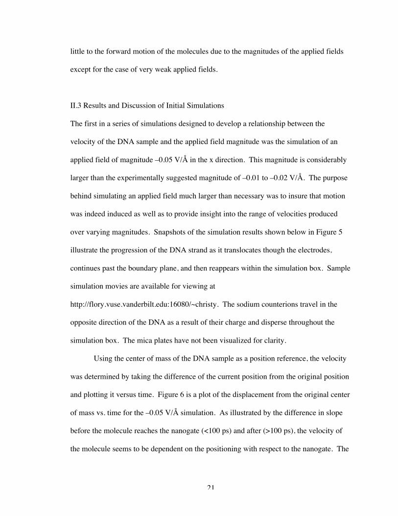
over varying magnitudes. Snapshots of the simulation results shown below in Figure 5
illustrate the progression of the DNA strand as it translocates though the electrodes,
continues past the boundary plane, and then reappears within the simulation box. Sample
simulation movies are available for viewing at
http://flory.vuse.vanderbilt.edu:16080/~christy. The sodium counterions travel in the
opposite direction of the DNA as a result of their charge and disperse throughout the
simulation box. The mica plates have not been visualized for clarity.
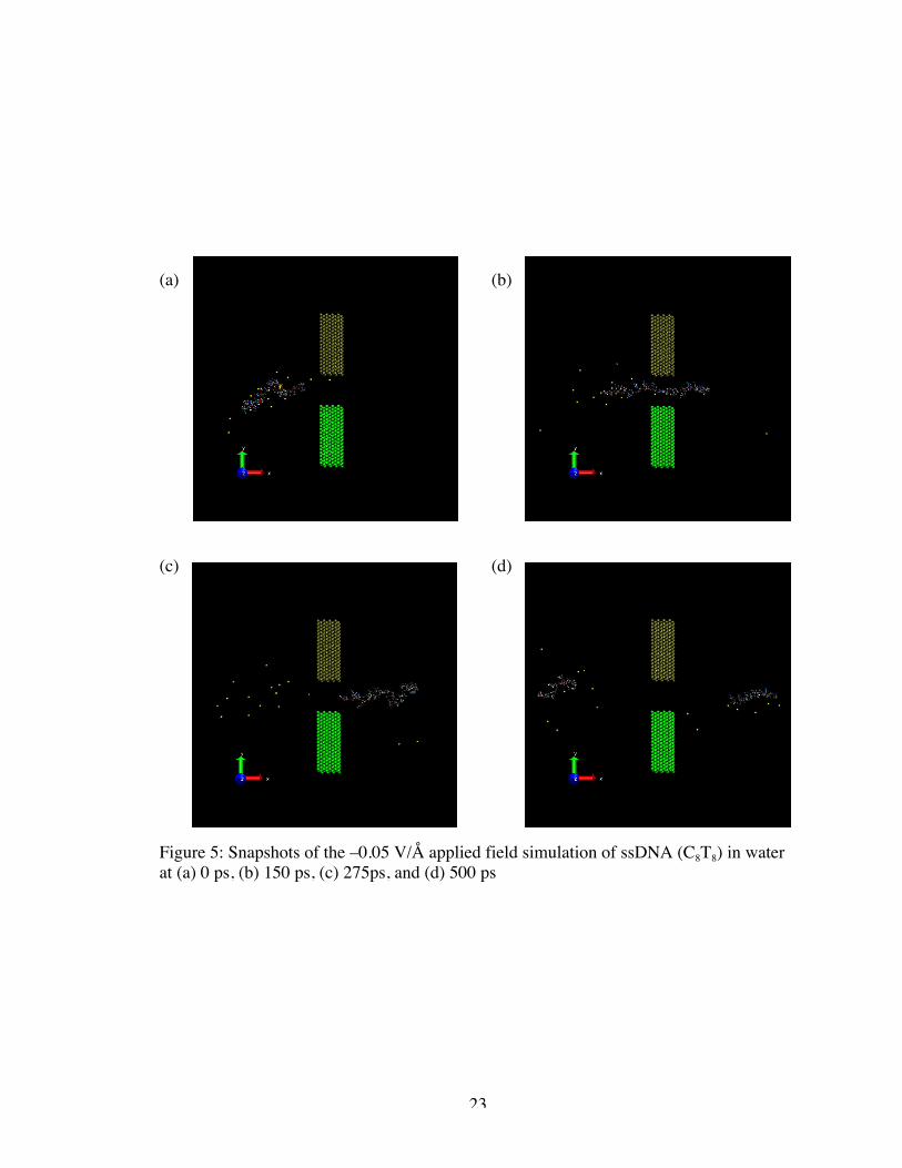
Using the center of mass of the DNA sample as a position reference, the velocity
was determined by taking the difference of the current position from the original position
and plotting it versus time. Figure 6 is a plot of the displacement from the original center
of mass vs. time for the –0.05 V/Å simulation. As illustrated by the difference in slope
before the molecule reaches the nanogate (<100 ps) and after (>100 ps), the velocity of
the molecule seems to be dependent on the positioning with respect to the nanogate. The

22
molecule appears to be traveling at a velocity of approximately 200 Å/ns before it
reaches the nanogate and increases velocity in the vicinity of the nanogate to 415 Å/ns.
These values are substantial departures from the desired value of 1 to 2 Å/ ns to µs. As
expected, there is little motion in y and z-directions of the simulation because the field
was applied in x-direction.
23
(a) (b)
(c) (d)
Figure 5: Snapshots of the –0.05 V/Å applied field simulation of ssDNA (C8T8) in waterat (a) 0 ps, (b) 150 ps, (c) 275ps, and (d) 500 ps
24
0
50
100
150
200
250
300
350
400
0 200 400 600 800 1000
xyz
Chan
ge in
Dire
ctio
n (Å
)
Time (ps)
Figure 6: Change in direction vs. time based on the center of mass with an appliedelectrical field of –0.05 V/Å.
25
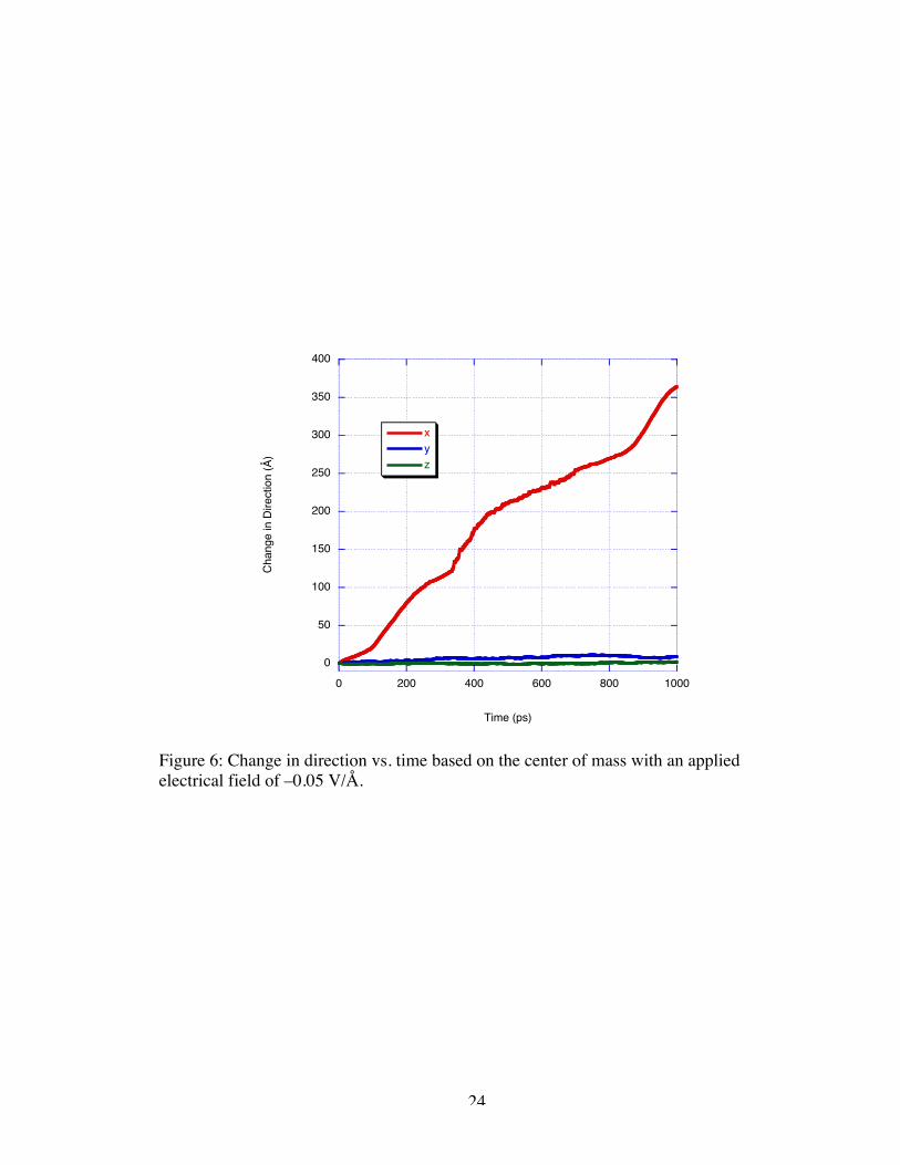
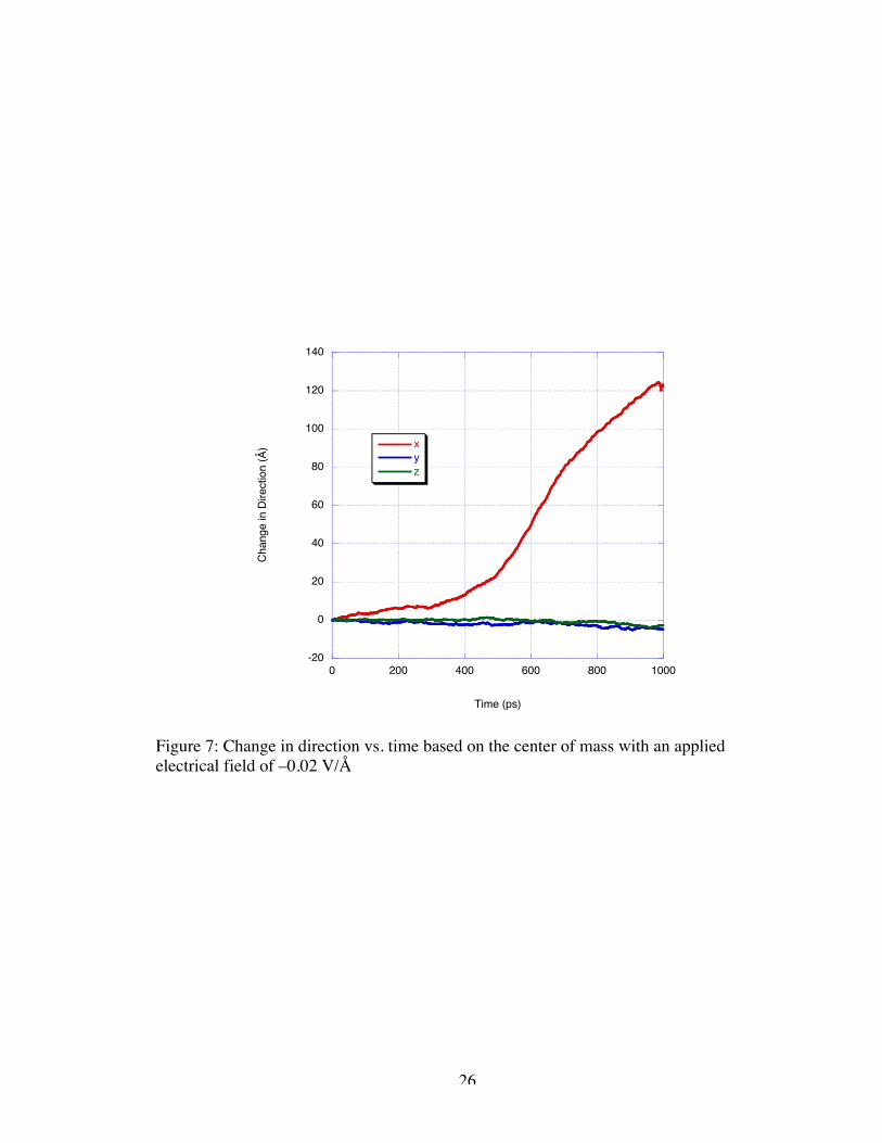
As a result of obtaining such remarkable velocity with the –0.05 V/Å applied
field, the next simulation in this series implemented a field of less than half that
magnitude at –0.02 V/Å. As expected, the lower magnitude electrical driving force
resulted in slower translocation of the DNA sample. The sample translocated through the
electrodes a single time in the case of the –0.02 V/Å field. Again, as illustrated in Figure
7, the velocity observed as calculated through the displacement from the original center
of mass position has two distinct regimes, bulk velocity and approaching translocation.
The bulk velocity appears to be around 50 Å/ns while the velocity increases to near 220
Å/ns as the DNA strand approaches and passes through the nanogate. Movement in the y
and z-directions is negligible in comparison to x-directional velocity. Like the resulting
velocity from the applied field of –0.05 V/Å, the induced velocity from the –0.02 V/Å
field is much larger than desired.
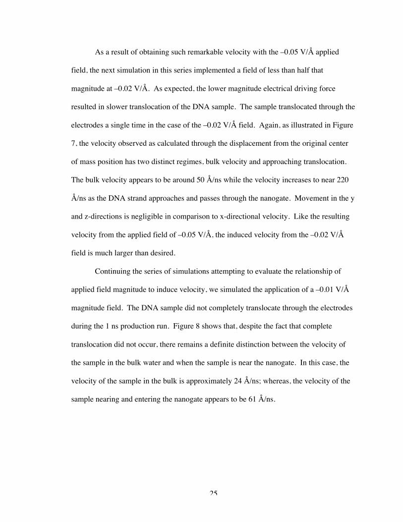
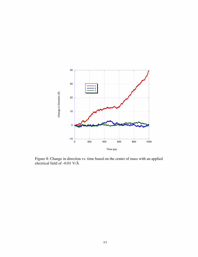
Continuing the series of simulations attempting to evaluate the relationship of
applied field magnitude to induce velocity, we simulated the application of a –0.01 V/Å
magnitude field. The DNA sample did not completely translocate through the electrodes
during the 1 ns production run. Figure 8 shows that, despite the fact that complete
translocation did not occur, there remains a definite distinction between the velocity of
the sample in the bulk water and when the sample is near the nanogate. In this case, the
velocity of the sample in the bulk is approximately 24 Å/ns; whereas, the velocity of the
sample nearing and entering the nanogate appears to be 61 Å/ns.
26
-20
0
20
40
60
80
100
120
140
0 200 400 600 800 1000
xyz
Chan
ge in
Dire
ctio
n (Å
)
Time (ps)
Figure 7: Change in direction vs. time based on the center of mass with an appliedelectrical field of –0.02 V/Å
27
-10
0
10
20
30
40
0 200 400 600 800 1000
xyz
Chan
ge in
Dire
ctio
n (Å
)
Time (ps)
Figure 8: Change in direction vs. time based on the center of mass with an appliedelectrical field of –0.01 V/Å
28
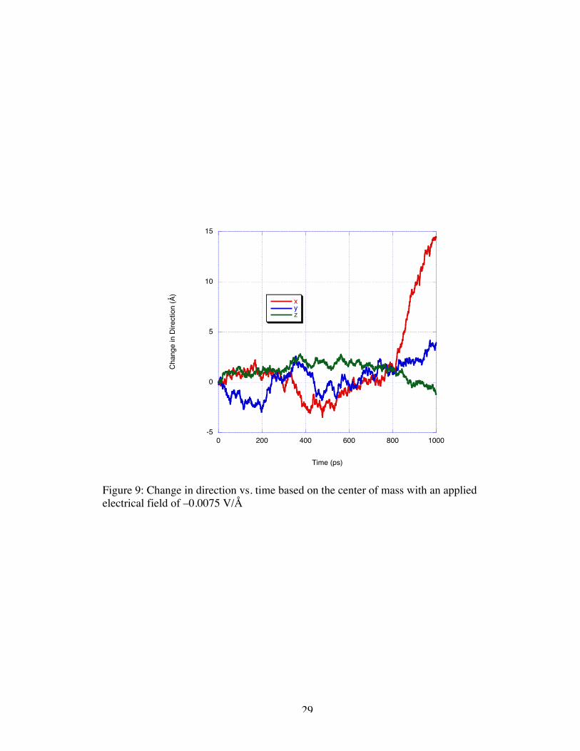
The next simulation in this series was that of an applied field of –0.0075 V/Å.
The –0.0075 V/Å magnitude applied field resulted in less definitive bulk motion in
comparison to previous simulations. As shown in Figure 9, the DNA seems to exhibit
somewhat oscillatory velocity at 4 Å/ns in the x-direction as the strand creeps toward the
nanogate over a period of 800 ps. When the sample reaches a point near the nanogate,
the velocity increases to approximately 65 Å/ns. This is roughly the same velocity in the
vicinity of the electrodes as the resulting velocity of a –0.01 V/Å applied field. Under
this lower magnitude applied field, the motion in the y and z-directions becomes more
noticeable; however, the application of an external field in the x-direction will override
motion in the y-direction. The z-direction is fixed due to the presence of the mica
surfaces above and below the sample solution.
Following the –0.0075 V/Å simulation with a –0.005 V/Å simulation, we are
presented with seemingly contradictory results. In Figure 10, one can see that the
oscillatory behavior at approximately 5 Å/ns reappears under the low magnitude applied
field; however, this behavior is only exhibited over 200 ps before the DNA reaches the
pull of the nanogate and increases in velocity to 19 Å/ns.
29
-5
0
5
10
15
0 200 400 600 800 1000
xyz
Chan
ge in
Dire
ctio
n (Å
)
Time (ps)
Figure 9: Change in direction vs. time based on the center of mass with an appliedelectrical field of –0.0075 V/Å
30
-5
0
5
10
15
20
0 200 400 600 800 1000
xyz
Chan
ge in
Dire
ctio
n (Å
)
Time (ps)
Figure 10: Change in direction vs. time based on the center of mass with an appliedelectrical field of –0.005 V/Å
31
Continuing to lower the magnitude of the applied field to –0.002 V/Å results in
entirely oscillatory motion of nearly the same velocity in all directions resulting in no
appreciable net motion as seen in Figure 11. This and the behavior of the –0.0075 V/Å
and –0.005 V/Å simulation leads to the conjecture that an apparent energy barrier to
motion exists which must be overcome before the molecule begins its approach to the
nanogate. It is my opinion that should the simulation of the –0.002 V/Å applied field be
continued beyond the 1 ns production run, the DNA molecule would eventually begin
progressing toward the electrodes as the molecule did previously under larger magnitude
fields.
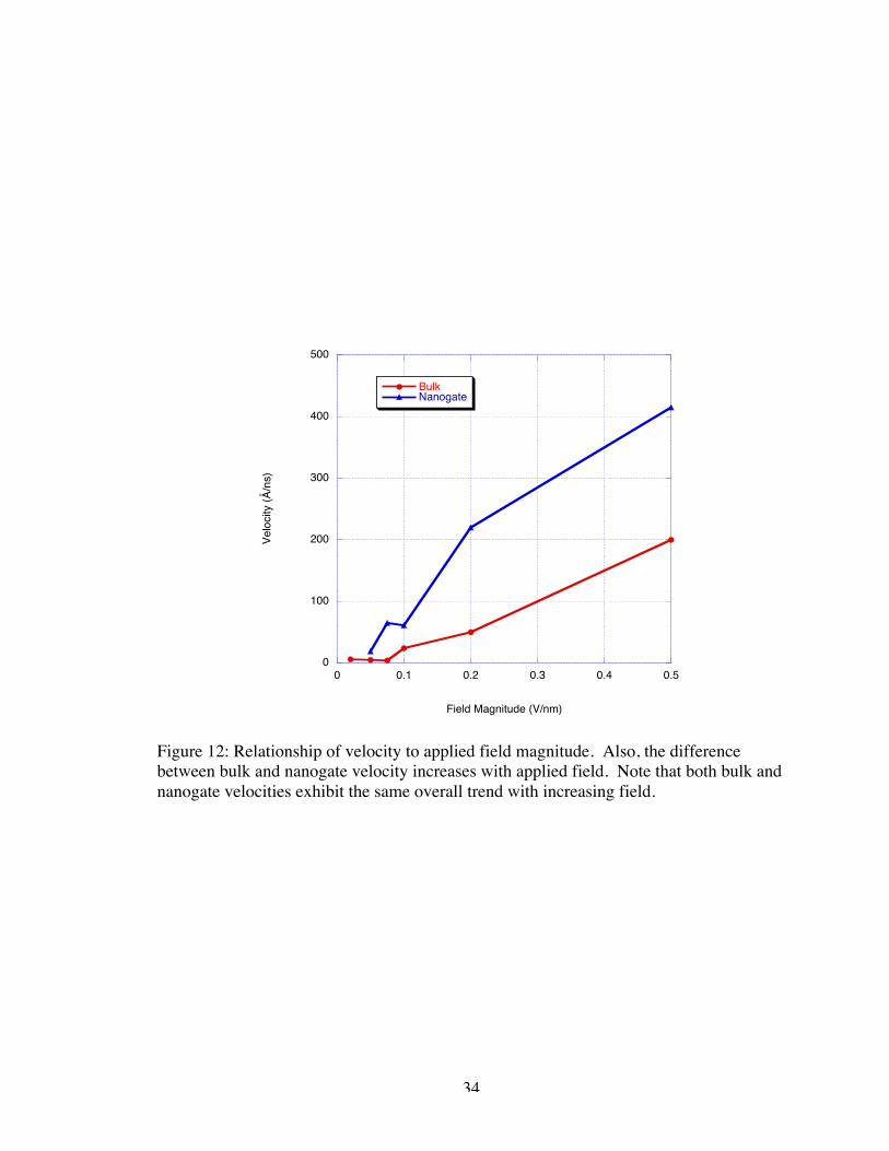
Examining the relationship of the magnitude of the electric field with respect to
the apparent velocity of the center of mass of the molecule requires examining both the
bulk velocity and the velocity in proximity of the nanogate. As previously shown, these
two situations within the simulation result in drastically different behaviors. Figure 12 is
a compilation of the velocities resulting from the above-mentioned simulations.
Position relative to the nanogate was delineated by the marked acceleration of the
molecule. The ssDNA molecules appeared to accelerate when the first base pair was
within 0.5 nm of the entrance to the gap. All molecules, with the exception of the
smallest magnitude applied electric field (-0.02 V/Å), entered the device gap to some
degree during the course of our simulations. This acceleration may be an artifact of the
force fields used for the DNA-electrode and water-electrode interactions37. According to
the results, the bulk velocity relationship to the electric field magnitude appeared to be
nearly linear, given the rough approximation of velocity, when the field strength was
32
stronger than –0.01 V/Å which was in agreement with previous similar simulations14;
however, under smaller magnitude fields, the motion fell into somewhat oscillatory
behavior, perhaps as a result of the short length of the simulation and possible energetic
barriers to translocation. The relationship of the velocity near the nanogate to the field
magnitude appeared to be nonlinear given the set of velocities available. One could
compare this to what is known for non-biological polymers translocating through
nanopores, for which a consensus on the expected behavior of polymers translocating
through nanopores has not been reached at this time. Over small ranges of applied fields,
the drift velocity of polymers varied linearly with potentials38; however, over wider
ranges, the relationship appeared to be more quadratic in form4. This could be attributed
to the large number of variables involved in determining this relationship such as the pore
material/polymer interactions, length of the polymer affecting velocity, and energetic
barriers to translocation in general. Despite my conjectures, definitive relationships
cannot be determined from this limited set of data.
33
-6
-4
-2
0
2
4
0 200 400 600 800 1000
xyz
Chan
ge in
Dire
ctio
n (Å
)
Time (ps)
Figure 11: Change in direction vs. time based on the center of mass with an appliedelectrical field of –0.002 V/Å
34
0
100
200
300
400
500
0 0.1 0.2 0.3 0.4 0.5
BulkNanogate
Velo
city
(Å/n
s)
Field Magnitude (V/nm)
Figure 12: Relationship of velocity to applied field magnitude. Also, the differencebetween bulk and nanogate velocity increases with applied field. Note that both bulk andnanogate velocities exhibit the same overall trend with increasing field.
35
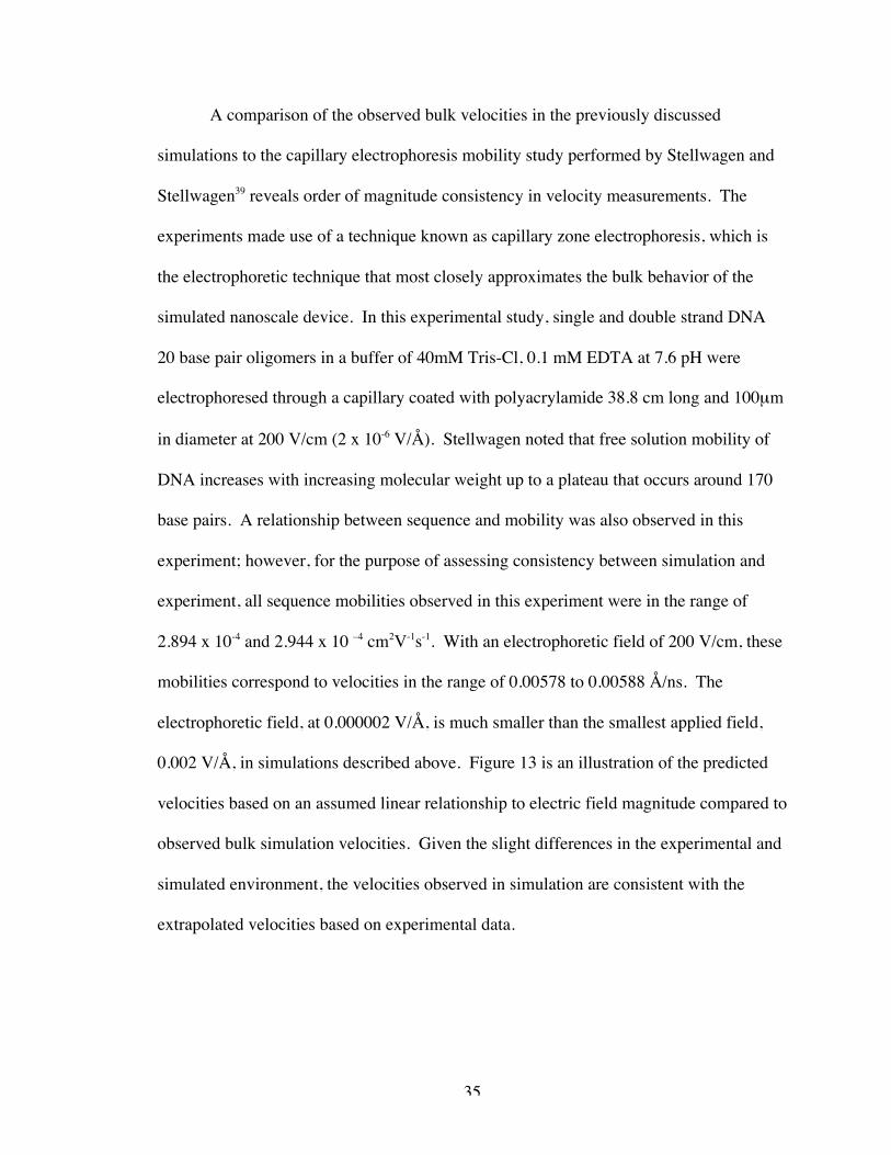
A comparison of the observed bulk velocities in the previously discussed
simulations to the capillary electrophoresis mobility study performed by Stellwagen and
Stellwagen39 reveals order of magnitude consistency in velocity measurements. The
experiments made use of a technique known as capillary zone electrophoresis, which is
the electrophoretic technique that most closely approximates the bulk behavior of the
simulated nanoscale device. In this experimental study, single and double strand DNA
20 base pair oligomers in a buffer of 40mM Tris-Cl, 0.1 mM EDTA at 7.6 pH were
electrophoresed through a capillary coated with polyacrylamide 38.8 cm long and 100µm
in diameter at 200 V/cm (2 x 10⁻⁶ V/Å). Stellwagen noted that free solution mobility of
DNA increases with increasing molecular weight up to a plateau that occurs around 170
base pairs. A relationship between sequence and mobility was also observed in this
experiment; however, for the purpose of assessing consistency between simulation and
experiment, all sequence mobilities observed in this experiment were in the range of
2.894 x 10⁻⁴ and 2.944 x 10 –4 cm2V-1s-1. With an electrophoretic field of 200 V/cm, these
mobilities correspond to velocities in the range of 0.00578 to 0.00588 Å/ns. The
electrophoretic field, at 0.000002 V/Å, is much smaller than the smallest applied field,
0.002 V/Å, in simulations described above. Figure 13 is an illustration of the predicted
velocities based on an assumed linear relationship to electric field magnitude compared to
observed bulk simulation velocities. Given the slight differences in the experimental and
simulated environment, the velocities observed in simulation are consistent with the
extrapolated velocities based on experimental data.
36
0
50
100
150
200
250
0 0.1 0.2 0.3 0.4 0.5
Simulation (Å/ns)Predicted (Å/ns)
Velo
city
(Å/n
s)
Electric Field Magnitude (V/nm)
Figure 13: Relationship of velocity to applied field magnitude in bulk solution comparedto velocities predicted based on electrophoretic experiments
37
An additional behavior of note observed in each simulation as the DNA sample
passes through the nanogate is molecular elongation. This is somewhat expected due to
the size of the nanogap at 2.87 nm. Furthermore, this may be a root cause of the increase
in velocity as the DNA translocates due to the repulsion forces created to achieve the
energetically favorable relaxed conformation after translocation. Elongation was
quantitatively observed by tabulating the end-to-end distance of the molecule as a
function of time as shown in Figure 14. In the event that the DNA sample enters the gap
between the electrodes, the end-to-end distance increases by almost 30 Å as the DNA
passes through the nanogate which is roughly 55% of the initial length. While the helix
geometry does not maintain rigidity, the molecular structure does not appear to stretch
beyond reasonable expectations. In the simulation of the –0.05 V/Å magnitude applied
field, this elongation pattern is observed twice as the molecule reentered the simulation
boundary and translocated a second time.
Additional analysis of factors such as the radius of gyration and the root mean
square distribution have thus far yielded no additional insights about the nature of motion
of the DNA sample.
38
40
50
60
70
80
90
100
0 200 400 600 800 1000
-0.5 V/nm-0.2 V/nm-0.1 V/nm-0.075 V/nm-0.05 V/nm-0.02 V/nm
End-
to-E
nd D
istan
ce (Å
)
Time (ps)
Figure 14: End-to-end distance vs. time of DNA under an applied electrical field
39
II.4 Interaction Potential for Metals and Non-metals
A significant fault of the preliminary simulations is the lack of an adequate interaction
potential for describing the behavior of non-metal atoms interacting with metal atoms. A
visualization of the equilibrated system in which the water molecules are shown, Figure
15, exemplifies the inadequate description. One can see how the metallic surface appears
hydrophobic and the water molecules form lower density pockets around the surface of
the metal.
One of the most important tasks to be accomplished within this project is to
properly implement a new potential into LAMMPS to account for the metal/non-metal
interactions. The current behavior of the water at the electrode surface may possibly be
interfering with the forward motion of the DNA molecule. Additionally, the repulsion
from the electrodes is not limited in its effects to water and may explain the reluctance of
the DNA strand to translocate under lower magnitude electric field application.
This behavior occurred because the implemented potential failed to properly
reproduce the varying charge density in response to Coulombic forces acting on the
metal. In the past, this has been accounted for by a method known as the image charge
method40. Spohr and Heinzinger41 have previously used this method successfully to
model the platinum/water interface; however, their implementation is only valid for
simple macroscopic geometries that cross the periodic boundary conditions essentially
producing infinite slabs.
This has been addressed by modifying LAMMPS based on the electrode charge
dynamics (ECD) method developed recently by Guymon, et al.42. We will discuss the
40
electrode charge dynamics methodology in more detail as well as limitations to its
implementations and the resulting simulations in a future chapter.
II.5 Magnitude and Velocity Relationship
A conclusion has yet to be made as to the relationship of the applied electric field
magnitude to resulting velocity of the DNA sample. It is clear that more simulations
must be performed to explore this relationship. With the new metal/non-metal potential
implemented, the –0.05, -0.02, -0.01, -0.0075, -0.005, and –0.002 V/Å applied field
simulations have been repeated extending the length of the simulations to 2 ns.
The task of simulating production runs to develop the magnitude/velocity
relationship will require re-equilibration using the newly implemented potential. Each
production run of 1 ns takes approximately two days to complete on 64 Opteron
processors.
41
Figure 15: Equilibrated device with visualized water molecules
42
II.6 Identify Optimal Controlling Mechanism
The possibility exists that the application of a uniform electric field will not be sufficient
to control the translocation of the DNA sample as intended. As mentioned before, the
implementation of a pulsed electric field within molecular dynamics would require
increased computational resources. This hurdle has forced our initial investigation into
controlling mechanisms to focus on inducing flow within the solution.
II.6.A Simulation Details
The physical setup of the simulated device was exactly the same as the setup used in the
electric field magnitude studies mentioned previously, including the use of the same
forcefields.
The induction of flow was achieved by imposing an additional external force of
equal magnitude on every atom in the solution. Production runs of 1 ns were performed
for each magnitude tested.
II.6.B Results and Discussion of Flow Simulations
Simulations were performed with 0.5, 0.25, 0.05, 0.005, and 0.0001 kcal/mol-Å
magnitude forces on the solution atoms. Assuming linear response behavior (i.e., that
Navier-Stokes hydrodynamics is valid), these forces correspond to very large pressure
drops (~ 0.5 MPa to 8 MPa over 20.7 nm) over the length of the simulation box;
however, with respect to molecular dynamics, these pressure drops are negligible in
comparison to fluctuations in pressure (~ 10 MPa) typically observed in molecular
dynamics simulations. The simulations of 0.5, 0.25, 0.05, and 0.005 kcal/mol-Å

43
magnitude forces all resulted in very similar behavior to varying degrees. Figure 16 is an
illustration of this behavior in which the forces on the solution atoms are so strong that
the stationary constraint imposed on the electrodes cannot be maintained. Additionally,
one can see that the solution atoms are moving so fast that they create void space behind
the electrodes. This is clearly too fast (~ 600 m/s) to be of use in the sequencing device.
44
(a) (b)
Figure 16: Snapshots of the 0.05 kcal/mol-Å magnitude force simulation of ssDNA(C8T8) in water at (a) 0 ps and (b) 1000 ps
45
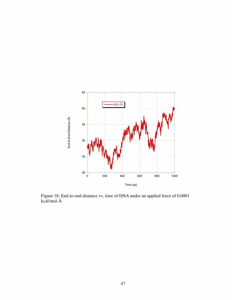
In contrast, the simulation of the 0.0001 kcal/mol-Å applied force produced much
more promising results. Not only did the applied force not create the void space behind
the nodes, the electrodes remained stationary objects within the simulation. As in the
applied electric field simulations, the velocity of the DNA strand was determined through
the evaluation of the change in direction of the center of mass from its original position.
Figure 17 is the plot of this change in direction for the 0.0001 kcal/mol-Å simulation.
The molecule appears to have net motion away from the initial position of about 1 Å;
however, the velocity varies over the course of the simulation.
Elongation of the DNA strand was noted as it was in the applied electrical field
simulations. The elongation in the 0.0001 kcal/mol-Å induced flow simulation was
similar to those observed in the applied field simulations. Note that applied electric field
should not elongate a uniformly charge object. The molecule’s end-to-end distance
increased by approximately 10 Å over the course of a nanosecond as shown in Figure 18.
More extreme elongation was not seen in this simulation likely because the molecule did
not come close enough to the nanogate.
Preliminary simulations provide promising results that indicate induced flow may
be used as a controlling mechanism. Ideally, more simulations of induced flow need to be
performed at a variety of magnitudes between 0.0001 kcal/mol-Å and 0.005 kcal/mol-Å,
implementing the proper metal/non-metal potential, to better understand the relationship
of magnitude to velocity. Furthermore, the implementation of pulsed applied electrical
fields should be examined should both uniform electrical field application and induced
flow prove incapable of producing the desired motion control; however, these
implementations are beyond the scope of this dissertation.
46
-1
0
1
2
3
4
0 200 400 600 800 1000
xyz
Chan
ge in
Dire
ctio
n (Å
)
Time (ps)
Figure 17: Change in direction vs. time based on the center of mass with an applied forceof 0.0001 kcal/mol-Å
47
40
45
50
55
60
65
0 200 400 600 800 1000
e2e (Å)
End-
to-E
nd D
istan
ce (Å
)
Time (ps)
Figure 18: End-to-end distance vs. time of DNA under an applied force of 0.0001kcal/mol-Å
48
CHAPTER III
ELECTROPHORETIC RESPONSE OF DNA IN SOLUTION
III.1 Motivation
Initial simulations of a given configuration of the conceptual device have shown that
DNA behaves differently in the bulk solution than it does when in proximity to the
electrode gate. Motivated by the similarity of the comparison of the transport properties
of the ssDNA molecule in bulk solution to experimental capillary electrophoresis data
and as part of the investigation into the ideal configuration of the sequencing device, we
decided to perform molecular dynamics simulations of ssDNA and dsDNA in a bulk
aqueous environment to directly compare the electrophoretic mobility calculated by
simulation to experiment. We will examine the relationship between simulated
electrophoretic mobility and experimental as a means of validating implemented force
fields.
The examination of simulated electrophoretic mobility will again make use of the
capillary zone electrophoresis mobility study performed by Stellwagen and Stellwagen39
for comparison. The experimental capillary zone electrophoresis technique is easily
approximated in simulation by the application of an external electric field. In this
experimental study, as described in the previous chapter, single and double strand DNA
20 base pair oligomers in a buffer of 40mM Tris-acetate-EDTA at 7.6 pH were
electrophoresed through a capillary coated with polyacrylamide 38.8 cm long and 100µm
in diameter at 200 V/cm (2 x 10⁻⁶ V/Å). Stellwagen noted that free solution mobility of
49
DNA increased with increasing molecular weight up to a plateau that occurred around
170 base pairs. A relationship between sequence and mobility was also observed in this
experiment; however, for the purpose of assessing consistency between simulation and
experiment, we focused on two oligomers. All sequence mobilities observed in this
experiment were in the range of 2.894 x 10⁻⁴ and 2.944 x 10⁻⁴ cm2V-1s-1. With an
electrophoretic field of 2 x 10⁻⁶ V/Å, these mobilities corresponded to velocities in the
range of 0.00578 to 0.00588 Å/ns.
III.2 Simulation Details
We performed a series of simulations of both single and double strand DNA molecules in
pure water similar to single-stranded RNA MD simulations performed by Yeh and
Hummer14 in order to more directly compare simulation results to experiment. The
experiment authors, Stellwagen and Stellwagen, electrophoresed several different
configurations of single strand DNA molecules as well as several double strand DNA
molecules. We chose to compare our simulations to the experimental results of
Stellwagen over another ssDNA electrophoretic mobility study by Hoagland43 because of
the smaller oligomers used in the Stellwagen study. Hoagland, et al. studied the
electrophoretic mobility of ssDNA molecules consisting of tens of thousands of base
pairs. This simulation study focused on the ssDNA oligomer denoted ssA5, which
consisted of the following sequence of nucleotides, CGCAAAAACGCGCAAAAACG,
as well as the dsDNA oligomer denoted dsA5, which was a double strand DNA molecule
consisting of the ssA5 sequence and its complement.
50
The MD simulations of ssA5 and dsA5 were performed using LAMMPS with the
CHARMM 27 all-hydrogen force field26, 27. Explicit water was described by the TIP3P
model29. The sodium counterions were represented by a potential developed by Beglov
and Roux28. Initial coordinates for the ssA5 and dsA5 molecules were generated using
Nucleic Acid Builder (NAB)44, 45. The molecules were solvated and neutralized with
sodium (Na+) counterions using a script within the LAMMPS software package. At a
density of 1 g/cc, 3802 water molecules solvated the ssA5 molecule in addition to 20
sodium counterions. The dsA5 molecule was solvated with 3486 water molecules and 40
sodium counterions.
The simulations utilized periodic boundary conditions and were equilibrated for
1ns using the NPT ensemble at 300 K and 101 325 Pa with the Nosé-Hoover thermostat46
and barostat47. Time integration was performed using the velocity-Verlet algorithm2 with
a timestep of 2 fs. The hydrogen bonds were constrained using the SHAKE algorithm48.
Long-range Coulombic interactions were computed using a particle-particle-particle-
mesh (PPPM) solver32.
After the equilibration period, the simulations were restarted with the addition of
an applied uniform external electric field of varying magnitudes (0.003, 0.03, 0.04, and
0.05 V/Å) and run for 1.5 ns. As in the previous simulations, these applied field
magnitudes were significantly larger than those typically used in capillary electrophoresis
experiments due to the timescale limitations of molecular simulation.
51
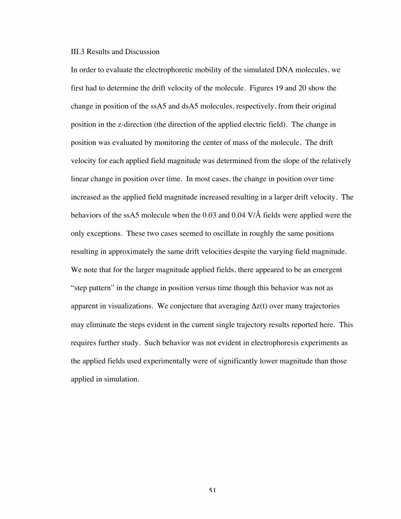
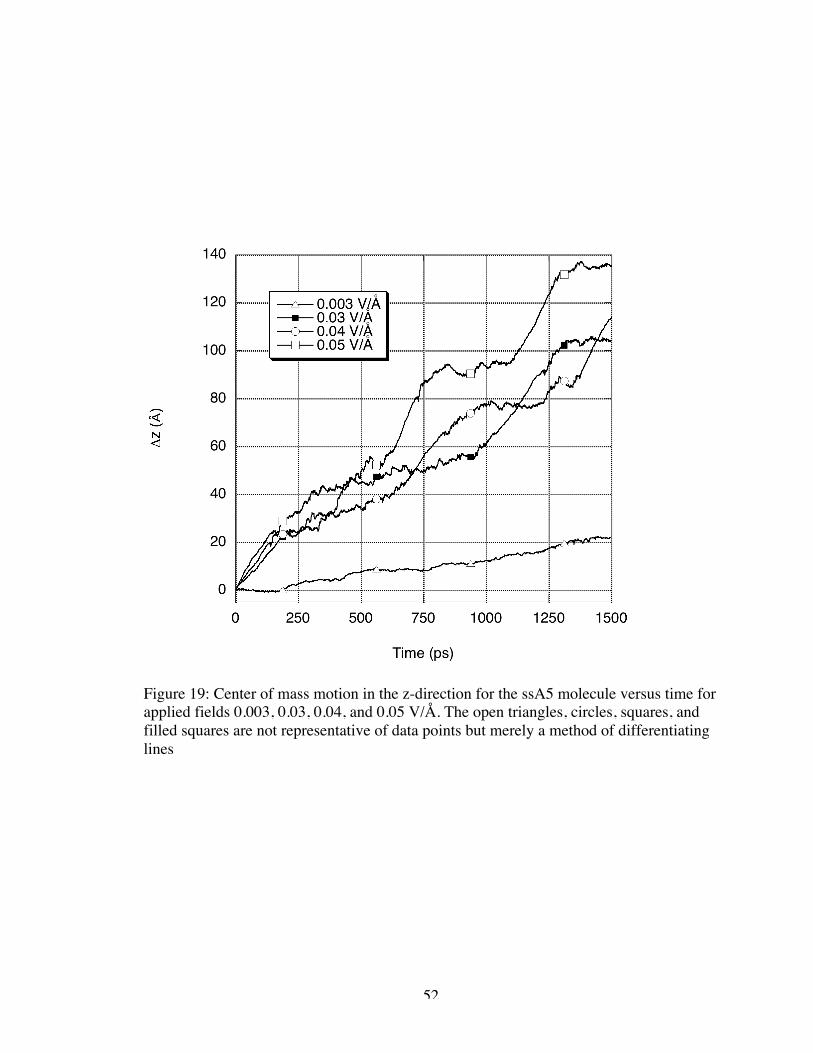
III.3 Results and Discussion
In order to evaluate the electrophoretic mobility of the simulated DNA molecules, we
first had to determine the drift velocity of the molecule. Figures 19 and 20 show the
change in position of the ssA5 and dsA5 molecules, respectively, from their original
position in the z-direction (the direction of the applied electric field). The change in
position was evaluated by monitoring the center of mass of the molecule. The drift
velocity for each applied field magnitude was determined from the slope of the relatively
linear change in position over time. In most cases, the change in position over time
increased as the applied field magnitude increased resulting in a larger drift velocity. The
behaviors of the ssA5 molecule when the 0.03 and 0.04 V/Å fields were applied were the
only exceptions. These two cases seemed to oscillate in roughly the same positions
resulting in approximately the same drift velocities despite the varying field magnitude.
We note that for the larger magnitude applied fields, there appeared to be an emergent
“step pattern” in the change in position versus time though this behavior was not as
apparent in visualizations. We conjecture that averaging Δz(t) over many trajectories
may eliminate the steps evident in the current single trajectory results reported here. This
requires further study. Such behavior was not evident in electrophoresis experiments as
the applied fields used experimentally were of significantly lower magnitude than those
applied in simulation.
52
Figure 19: Center of mass motion in the z-direction for the ssA5 molecule versus time forapplied fields 0.003, 0.03, 0.04, and 0.05 V/Å. The open triangles, circles, squares, andfilled squares are not representative of data points but merely a method of differentiatinglines
53
.
Figure 20: Center of mass motion in the z-direction for the dsA5 molecule versus time forapplied fields 0.003, 0.03, 0.04, and 0.05 V/Å. The open triangles, circles, squares, andfilled squares are not representative of data points but merely a method of differentiatinglines
54
Figure 21 illustrates the correlation of the drift velocities obtained as above with the
applied electric field. There is an assumed linear relationship between electric field
magnitude,
€
r E , and drift velocity,
€
r v , where the electrophoretic mobility, µ, is a
proportionality constant, i.e.
€
r v = µr E (6)
Based on this relationship, we have extrapolated an experimental drift velocity for each
of the simulated electric field magnitudes for comparison to simulated drift velocity. As
one can see, the simulated drift velocities were somewhat lower than the extrapolated
experimental values for the larger magnitude electric fields; however, the simulated drift
velocities of both ssA5 and dsA5 for the 0.003 V/Å magnitude were consistent with
experiment.
55
Figure 21: Drift velocity of ssA5 and dsA5 as a function of applied electric field. Thedashed and dot-dashed lines are the linear fits of the ssA5 and dsA5 drift velocity vs.electric field data, respectively, through which electrophoretic mobility was determined.The experimental velocities are obtained from Equation (6) using the experimentalelectrophoretic mobilities.
56
The values of the simulated electrophoretic mobility were calculated from the
slope of the linear fit to the drift velocity data. Significantly strong electric fields can
result in nonlinear electrophoretic mobilities49; however, in experimental capillary
electrophoresis and in this simulation study, the linear regime was applicable. Here,
electrophoretic mobility from simulation was calculated to be 1.8 x 10⁻⁴ and 9.8 x 10⁻⁵
cm2 V-1 s-1 for ssA5 and dsA5, respectively. Compared with the experimental values for
ssA5 at 2.87 x 10⁻⁴ and dsA5 at 2.89 x 10⁻⁴ cm2 V-1 s-1, we can see that simulation in the
above described manner resulted in a lower electrophoretic mobility (by 35% for ssA5
and by 65% for dsA5). This could result from the viscosity difference of using pure
water as the solvent in simulations as opposed using the buffer used in experiments.
Additionally, the simulations had no physical boundary such as the experimental
capillary, which could augment mobility, though in theory, this effect was corrected for
in the experiments. Of more concern was that the simulated electrophoretic mobility of
the larger molecule, dsA5, was smaller than that for the ssA5 molecule, while the
experimental observations indicated that the larger molecule should have a slightly larger
mobility. The experimental results were counter-intuitive (i.e., the experimental result
indicated that the larger molecule had slightly higher mobility), and so the significance of
the disagreement in the trends between simulation and experiment was difficult to gauge.
Additionally, we note that the experimental mobilities for ss and dsDNA may not be
statistically significantly different, once error estimates were taken into account. Though
Stellwagen and Stellwagen reported no error values for the normalized mobilities, error
propagation of the measured values to the normalized values used in this study indicated
that the mobilities of both dsA5 and ssA5 were statistically the same.
57
It is interesting to note that the mobilities calculated in the bulk simulations (i.e.,
with no nanogate present) were lower than those found in the bulk regime of the nanogate
simulation. One possibility was that the convective motion induced in the solvent by the
field acting on the DNA and its counterions was enhanced in the presence of the nanogate
because of the collimating effect of the nanogate, thus resulting in greater directionality
of the DNA motion in the direction of the applied field. This could be tested by
simulations in the presence of the nanogate in which the field is applied perpendicular to
the nanogate opening.
III.4 Conclusions
We have performed simulations of two DNA molecules, ssA5 and dsA5, in bulk aqueous
solution using classical molecular dynamics simulations in order to determine
electrophoretic mobilities. Results from the ssA5 and dsA5 simulations in bulk water
compared to initial simulations of ssDNA confined between two mica plates and
experimental capillary electrophoresis experiments were inconsistent at larger applied
electric field magnitudes. The simulated electrophoretic mobilities were notably smaller
likely due to freedom of motion through periodic boundary conditions. Future work in
this area will include the constraint of the DNA molecules in the x and y-directions as
well as examining lower magnitude fields over longer timescales.
58
CHAPTER IV
MOLECULAR DYNAMICS SIMULATION OF ssDNA TRANSLOCATIONTHROUGH A COPPER NANOELECTRODE GAP
Given the results from the initial molecular dynamics study of the proposed
genomic sequencing device, we decided to perform further simulations to evaluate the
applicability of the metal/non-metal interaction potential. Using a fixed gap width
between the electrodes and a small sample segment of ssDNA as initial starting points in
this portion of the project, the effect of applied electric fields on translocation velocity
was studied.
Research very similar to the proposed nanoscale sequencing device we will
evaluate in this work has been reported using the classical UFF31 potential for the
interaction of the metal electrodes with water, ions, and DNA 17; however, as we shall
see below, by implementing a more appropriate metal/non-metal interaction potential
known as electrode charge dynamics (ECD)42 we obtain more realistic results as
evidenced by water distributions around the metal nanoelectrodes and details of the
translocation velocities measured in the simulations. Our initial studies of DNA
molecules translocating through metallic electrodes have also made use of UFF in
describing metal/non-metal interactions of the metal with water, ions, and DNA.
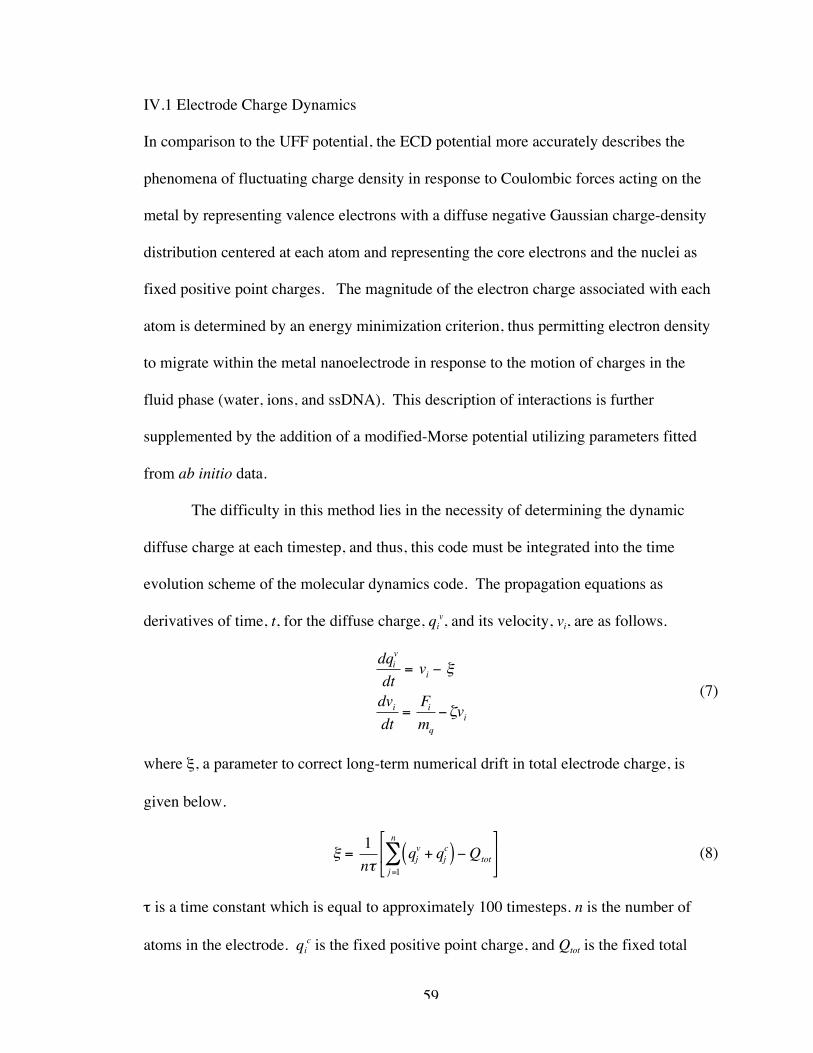
59
IV.1 Electrode Charge Dynamics
In comparison to the UFF potential, the ECD potential more accurately describes the
phenomena of fluctuating charge density in response to Coulombic forces acting on the
metal by representing valence electrons with a diffuse negative Gaussian charge-density
distribution centered at each atom and representing the core electrons and the nuclei as
fixed positive point charges. The magnitude of the electron charge associated with each
atom is determined by an energy minimization criterion, thus permitting electron density
to migrate within the metal nanoelectrode in response to the motion of charges in the
fluid phase (water, ions, and ssDNA). This description of interactions is further
supplemented by the addition of a modified-Morse potential utilizing parameters fitted
from ab initio data.
The difficulty in this method lies in the necessity of determining the dynamic
diffuse charge at each timestep, and thus, this code must be integrated into the time
evolution scheme of the molecular dynamics code. The propagation equations as
derivatives of time, t, for the diffuse charge, qiv, and its velocity, vi, are as follows.
€
dqiv
dt= vi − ξ
dvidt
=Fimq
−ζvi (7)
where ξ, a parameter to correct long-term numerical drift in total electrode charge, is
given below.
€
ξ =1nτ
qjv + qj
c( )j=1
n
∑ −Qtot
(8)
τ is a time constant which is equal to approximately 100 timesteps. n is the number of
atoms in the electrode. qic is the fixed positive point charge, and Qtot is the fixed total
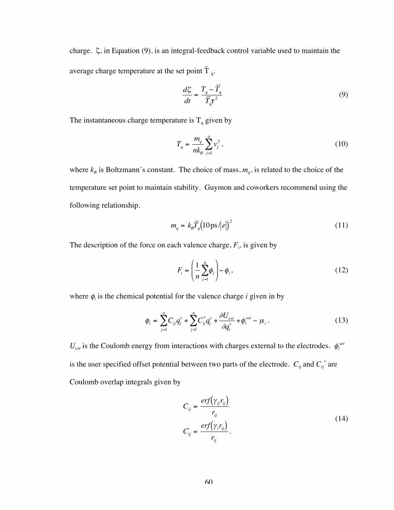
60
charge. ζ, in Equation (9), is an integral-feedback control variable used to maintain the
average charge temperature at the set point T̄ q.
€
dζdt
=Tq − T q
T qτ2 (9)
The instantaneous charge temperature is Tq given by
€
Tq =mq
nkBvj2
j=1
n
∑ , (10)
where kB is Boltzmann’s constant. The choice of mass, mq, is related to the choice of the
temperature set point to maintain stability. Guymon and coworkers recommend using the
following relationship.
€
mq = kBT q 10ps / e( )2 (11)
The description of the force on each valence charge, Fi, is given by
€
Fi =1n
φjj=1
n
∑
−φi , (12)
where φi is the chemical potential for the valence charge i given in by
€
φi = Cijqjv + Cij
*qjc +∂Uext
∂qiv +φi
set − µ ij=1
n
∑j=1
n
∑ . (13)
Uext is the Coulomb energy from interactions with charges external to the electrodes. φiset
is the user specified offset potential between two parts of the electrode. Cij and Cij* are
Coulomb overlap integrals given by
€
Cij =erf γ ij rij( )
rij
Cij* =
erf γ i rij( )rij
, (14)
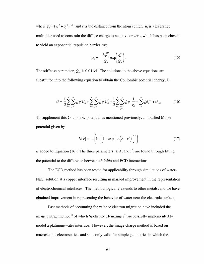
61
where γij = (γi-2 + γj
-2)-1/2, and r is the distance from the atom center. µi is a Lagrange
multiplier used to constrain the diffuse charge to negative or zero, which has been chosen
to yield an exponential repulsion barrier, viz
€
µ i = −kBT qQu
exp qiv
Qu
. (15)
The stiffness parameter, Qu, is 0.01 |e|. The solutions to the above equations are
substituted into the following equation to obtain the Coulombic potential energy, U.
€
U =12
qivqj
vCij + qivqj
cCij* +12
qicqj
c 1rij
+ qivφi
set
i=1
n
∑ +Uextj=1,j≠i
n
∑i=1
n
∑j=1
n
∑i=1
n
∑j=1
n
∑i=1
n
∑ (16)
To supplement this Coulombic potential as mentioned previously, a modified Morse
potential given by
€
U r( ) = −ε 1− 1− exp −A r − r *( )[ ]{ }2
(17)
is added to Equation (16). The three parameters, ε, A, and r*, are found through fitting
the potential to the difference between ab initio and ECD interactions.
The ECD method has been tested for applicability through simulations of water-
NaCl solution at a copper interface resulting in marked improvement in the representation
of electrochemical interfaces. The method logically extends to other metals, and we have
obtained improvement in representing the behavior of water near the electrode surface.
Past methods of accounting for valence electron migration have included the
image charge method40 of which Spohr and Heinzinger41 successfully implemented to
model a platinum/water interface. However, the image charge method is based on
macroscopic electrostatics, and so is only valid for simple geometries in which the
62
surface crosses periodic boundaries resulting in an infinite slab, essentially eliminating its
applicability to nanoscopic (i.e., non-macroscopic) metal objects. Hence, the ECD
method offers a significant opportunity for more accurate descriptions of ion-metal,
water-metal and ssDNA-metal interactions in realistic sequencing device configurations.
Initial simulations similar to the previously mentioned work utilizing the UFF
potential will be compared to simulations utilizing the alternate ECD potential. We
demonstrate that the choice of interaction potential between the metal and water
significantly impacts the behavior of the electrically driven DNA translocation behavior.
IV.2 Computational Method
The classical molecular dynamics simulations were performed using a modified version
of the LAMMPS (Large-scale Atomic/Molecular Massively Parallel Simulator)24, 25
simulation package. The LAMMPS code was modified and extended to incorporate ECD.
This procedure included the definition of new pair potentials for metal-metal and metal-
solution interactions with Gaussian type charge distributions, a new charge dynamics
class with methods controlling the amount of negative charge located at individual metal
atoms, and additional variables carrying atomic properties required by the ECD method,
such as chemical potential. The proper function of the code was tested by comparison
with the data published in the original paper42 and to independent simulations run with
our own in-house code which implements ECD.
The initial set of simulations was of a nanoscale sequencing device consisting of
two mica plates separated by approximately 3 nm; the solvated DNA and water are
enclosed between the plates. Each plate measured 20.7 nm x 14.4 nm. The detection
63
nodes were constructed of two copper FCC lattices measuring approximately 2 nm x 5
nm x 3 nm and separated by a 2.87 nm gap, as measured from center-to-center of the
outermost copper atoms. Copper nanoelectrodes, rather than the Pt and Au
nanoelectrodes being fabricated for the actual device, were used in this study since Cu is
the only metal for which ECD parameters have been published to date42. Obtaining ECD
parameters requires extensive ab initio calculations; the ECD interaction plus a Morse
potential are then used to extract the parameters required for the ECD model42. At the
moment, the 2.87 nm gap has been the only gap distance evaluated through simulation.
Future simulations will investigate the gap size, as well as other developmental design
details, including developing ECD parameters for metals other than Cu. The ssDNA
strand used in the present study consisted of sixteen nucleotides, eight consecutive
cytosines followed by eight consecutive thymines. The ssDNA was solvated in water at a
density of 1g/cc. The ssDNA strand was surrounded by sodium ions to make the total
system charge neutral. The number of atoms in this simulation totaled 132,697. The
total dimension of the simulation box was 20.7 nm x 14.4 nm x 5.0 nm (including mica
atoms). The simulations were periodic in the x and y directions and fixed in the z
direction represented in LAMMPS as a slab separated by a large vacuum space. Note
that the mica surfaces were parallel to the x-y plane.
Interaction potentials varied based on the atom type. The nucleic acids were
described using the CHARMM27 all-hydrogen potential26, 27. The sodium ions were
represented by a potential developed by Beglov and Roux28, included in the CHARMM
potential. Water molecules were described by the rigid water model known as TIP3P29
with which the CHARMM potential has been optimized. A more rigorous water
64
potential was unnecessary in comparison to the need for computational efficiency for
such a large system. The mica surfaces and the copper nodes were treated as rigid bodies
in this set of simulations. As such, their interactions with other atoms were estimated by
Lennard-Jones potential with parameters determined by Lorentz-Berthelot mixing rules.
The CLAYFF potential30 parameters were used for mica, and the UFF potential
parameters were used for copper. Note that, according to the experimental studies of
Klein50 and the simulations of Leng and Cummings51, 52, fluidity of water confined
between two mica surfaces is maintained under extreme confinement (down to mica-to-
mica separations of 0.7nm). The mica-to-mica distance used in this study was
approximately 3 nm, and so was much larger than the distances at which
nanoconfinement influences the fluidity of liquid water. Thus, based on these results50-
52we expect that the behavior of the water confined between the mica sheets will be bulk-
like.
All simulations began with an equilibration period of 1 ns. Simulations were
performed using the NVT ensemble at 300K with a Nosé-Hoover thermostat46. Time
integration was performed using the velocity-Verlet algorithm with a 2 fs timestep2.
Hydrogen bonds were constrained using the SHAKE algorithm48. The particle-particle
particle-mesh (PPPM) solver was used to compute long-range Coulombic interactions32.
The ssDNA strand was positioned at the entrance of the gap between the electrodes,
which will be referred to here as the nanogate. This positioning alleviated the need to
examine ssDNA conformational effects on the transport behavior. Experimentally, proper
alignment of the ssDNA strand to ensure translocation will have to be addressed, most
likely through the use of nanofluidic transport to the nanogate.
65
After the equilibration period, the simulations were subjected to an applied
uniform electric field and performed for 2 ns. This uniform field was applied in the x-
direction in order to force the ssDNA to translocate through the nanoscale gap. In an
attempt to develop a relationship between translocation velocity and magnitude of the
applied electric field, the field was varied between 0.0005 V/Å and 0.5 V/Å. In the actual
device, the electric field is better described as an effective potential varying based on
position within the device. The applied fields (0.0005, 0.001, 0.0025, 0.005, 0.0075,
0.01, 0.02, and 0.05 V/Å) correspond to effective transmembrane voltages drops of 1, 2,
5, 10, 15, 20, 40, and 100 mV; however, for the purpose of describing the relationship to
velocity, we will refer to the applied field magnitude. In the future, examining pulsing
electric fields as a driving force would be desirable though extremely computationally
expensive. Additionally, the proper positioning of the ssDNA strand between the
electrodes may necessitate the use of a holding field perpendicular to the mica surface.
A second set of simulations was performed exchanging the UFF potential used to
describe the metal/non-metal interactions by the more appropriate ECD potential. Based
on the UFF simulations, the size of the simulation box was reduced to obtain more
efficiently information about transport behavior (in essence, to eliminate some of the bulk
water that did not contribute to transport). In this case, the simulation box was 15.6 nm x
14.4 nm x 5 nm totaling 107, 545 atoms. All other simulation details remained the same
as described for the initial simulation set.
Due to the intense computational requirements of simulations this size, the
following results shown are of single trajectories. While ensemble averages would be
useful in generalizing behavior, we believe that the results presented still properly
66
illustrate the transport phenomena, and in particular, demonstrate clearly the impact of
the use of ECD.
IV.3 Results
This section presents results first from the simulations utilizing the UFF potential and
second from the simulations utilizing the ECD methodology. The resulting translocation
velocity and relationships to applied electric field are studied and compared.
IV.3.A. UFF Potential
The results in this section make use of the UFF potential as described in the methodology
section. This potential was initially chosen to represent the metal/non-metal interactions
in part because of its wide use53-57, its availability in existing molecular dynamics
software packages, in addition to its relative simplicity, while accepting its limitations in
describing variable charge density in metallic surfaces.
A significant goal of this project is to develop a relationship between translocation
velocity of the ssDNA sample and the applied electric field magnitude. In doing so, the
transport behavior of the ssDNA strand was evaluated over the application of eight
electric fields of magnitudes 0.0005, 0.001, 0.0025, 0.005, 0.0075, 0.01, 0.02, and 0.05
V/Å. Using the center of mass of the ssDNA strand as a position reference, the change in
position was determined by taking the difference of the current position from the original
position and plotting this difference versus time thus making the slope the resulting
translocation velocity. Figure 22 is the plot of the change in center of mass in the x-
direction as a function of time for the set of UFF simulations. The magnitude of the
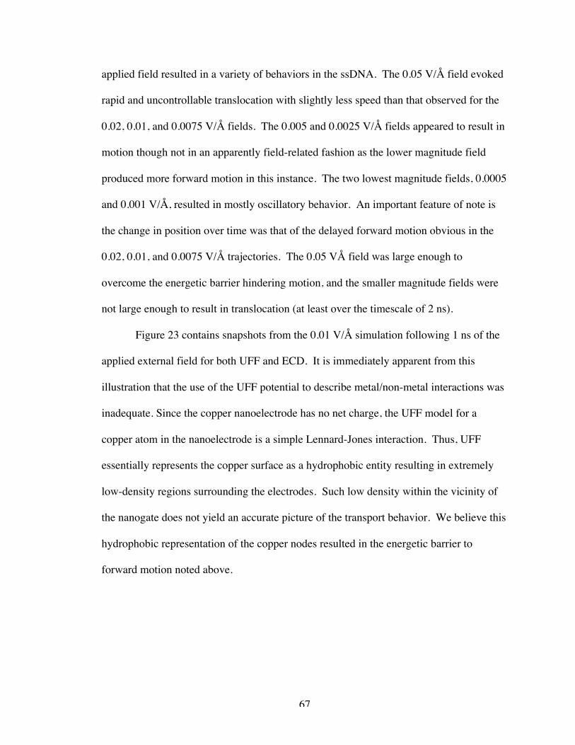
67
applied field resulted in a variety of behaviors in the ssDNA. The 0.05 V/Å field evoked
rapid and uncontrollable translocation with slightly less speed than that observed for the
0.02, 0.01, and 0.0075 V/Å fields. The 0.005 and 0.0025 V/Å fields appeared to result in
motion though not in an apparently field-related fashion as the lower magnitude field
produced more forward motion in this instance. The two lowest magnitude fields, 0.0005
and 0.001 V/Å, resulted in mostly oscillatory behavior. An important feature of note is
the change in position over time was that of the delayed forward motion obvious in the
0.02, 0.01, and 0.0075 V/Å trajectories. The 0.05 VÅ field was large enough to
overcome the energetic barrier hindering motion, and the smaller magnitude fields were
not large enough to result in translocation (at least over the timescale of 2 ns).
Figure 23 contains snapshots from the 0.01 V/Å simulation following 1 ns of the
applied external field for both UFF and ECD. It is immediately apparent from this
illustration that the use of the UFF potential to describe metal/non-metal interactions was
inadequate. Since the copper nanoelectrode has no net charge, the UFF model for a
copper atom in the nanoelectrode is a simple Lennard-Jones interaction. Thus, UFF
essentially represents the copper surface as a hydrophobic entity resulting in extremely
low-density regions surrounding the electrodes. Such low density within the vicinity of
the nanogate does not yield an accurate picture of the transport behavior. We believe this
hydrophobic representation of the copper nodes resulted in the energetic barrier to
forward motion noted above.
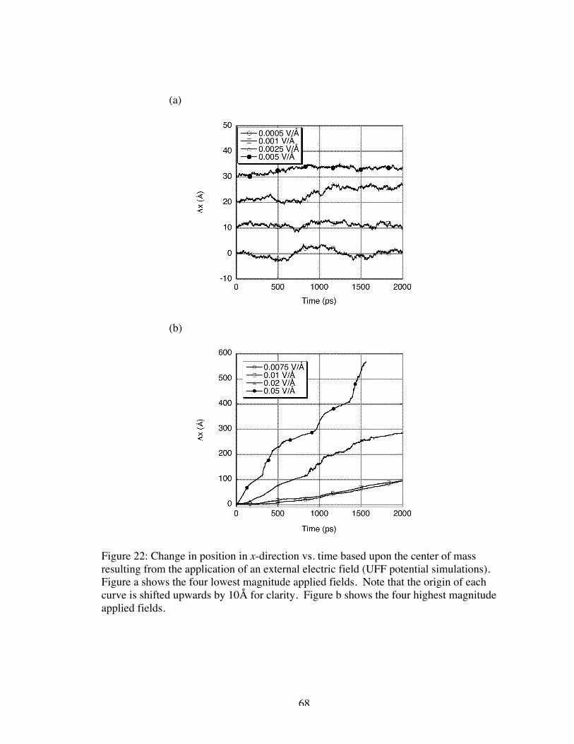
68
(a)
(b)
Figure 22: Change in position in x-direction vs. time based upon the center of massresulting from the application of an external electric field (UFF potential simulations).Figure a shows the four lowest magnitude applied fields. Note that the origin of eachcurve is shifted upwards by 10Å for clarity. Figure b shows the four highest magnitudeapplied fields.
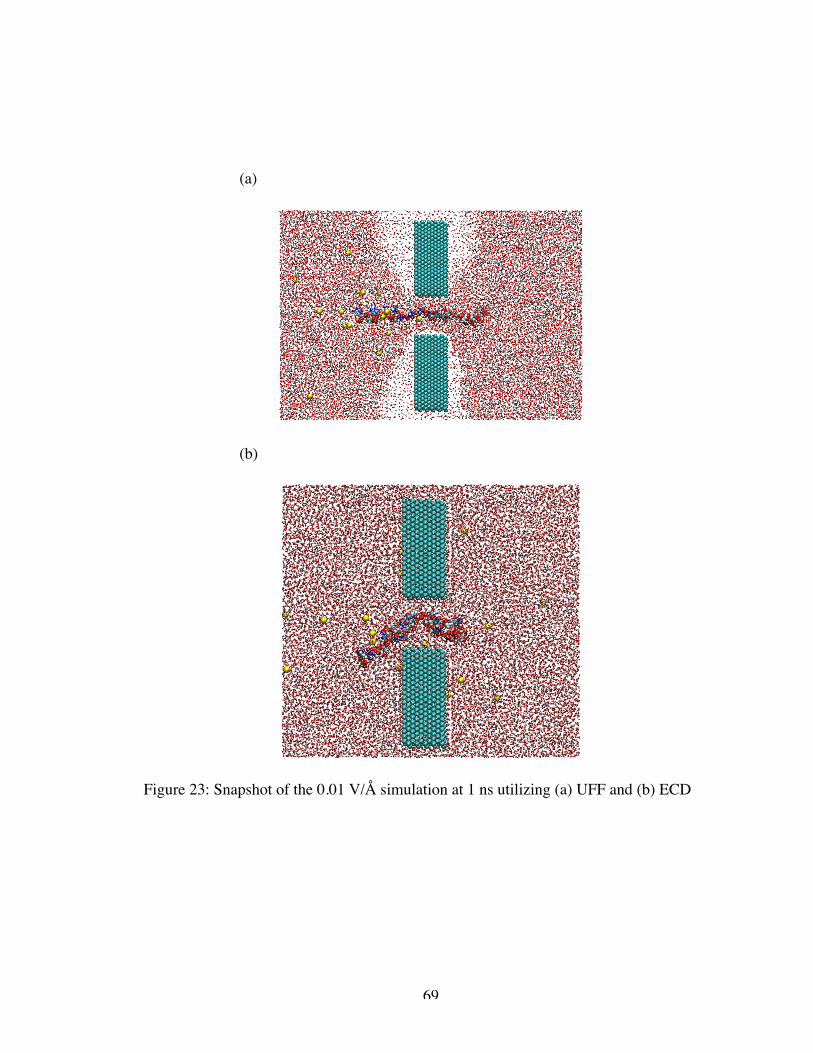
69
(a)
(b)
Figure 23: Snapshot of the 0.01 V/Å simulation at 1 ns utilizing (a) UFF and (b) ECD
70
IV.3.B. ECD Method
To address the significant shortcomings of the initial simulations resulting from the use
of the UFF potential, we performed the same set of simulations with the more appropriate
ECD potential in its place. It is apparent from visualization alone that the new potential
has much improved the physical behavior of non-metals in the presence of the copper
electrodes. The water molecules no longer formed low-density regions, more closely
resembling actual experimental operating conditions, as shown in Figure 23(b). Further
discussion of the density profiles resulting from both potential implementations will be
presented below.
Using the same method of determining change of position mentioned previously,
we have obtained Figures 24(a) and 24(b), which are plots of the change in position of
the center of mass in the x-direction over time for the simulations utilizing the ECD
potential. Note that the applied electric field was also applied to the electrodes, resulting
in a response within the Cu nanoelectrode. An immediately noticeable difference in the
trajectories compared to the UFF trajectories is that the lower magnitude applied fields
resulting in forward motion, as opposed to oscillatory behavior, have done so from the
beginning of the field application. The implementation of the ECD potential has most
notably eliminated the energetic barrier to motion observed in the initial set of
simulations. We expect that this was partly due to the charge polarization of the
nanoelectrodes, which should result in an additional attractive interaction between the
nanoelectrodes and the (negatively charged) ssDNA. As one would expect, the
application of an external electric driving force resulted in the immediate response of the
ssDNA strand and a more linear trajectory within the appropriate regime. Over the course
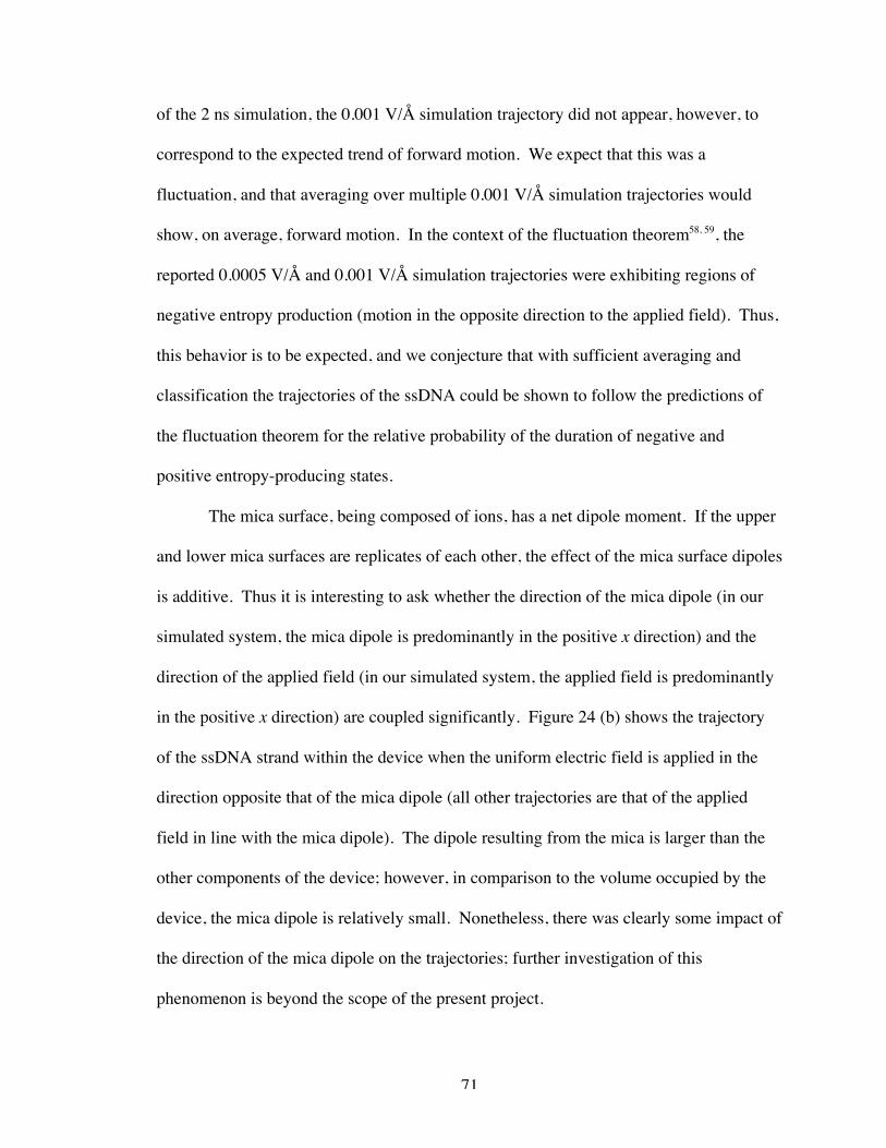
71
of the 2 ns simulation, the 0.001 V/Å simulation trajectory did not appear, however, to
correspond to the expected trend of forward motion. We expect that this was a
fluctuation, and that averaging over multiple 0.001 V/Å simulation trajectories would
show, on average, forward motion. In the context of the fluctuation theorem58, 59, the
reported 0.0005 V/Å and 0.001 V/Å simulation trajectories were exhibiting regions of
negative entropy production (motion in the opposite direction to the applied field). Thus,
this behavior is to be expected, and we conjecture that with sufficient averaging and
classification the trajectories of the ssDNA could be shown to follow the predictions of
the fluctuation theorem for the relative probability of the duration of negative and
positive entropy-producing states.
The mica surface, being composed of ions, has a net dipole moment. If the upper
and lower mica surfaces are replicates of each other, the effect of the mica surface dipoles
is additive. Thus it is interesting to ask whether the direction of the mica dipole (in our
simulated system, the mica dipole is predominantly in the positive x direction) and the
direction of the applied field (in our simulated system, the applied field is predominantly
in the positive x direction) are coupled significantly. Figure 24 (b) shows the trajectory
of the ssDNA strand within the device when the uniform electric field is applied in the
direction opposite that of the mica dipole (all other trajectories are that of the applied
field in line with the mica dipole). The dipole resulting from the mica is larger than the
other components of the device; however, in comparison to the volume occupied by the
device, the mica dipole is relatively small. Nonetheless, there was clearly some impact of
the direction of the mica dipole on the trajectories; further investigation of this
phenomenon is beyond the scope of the present project.
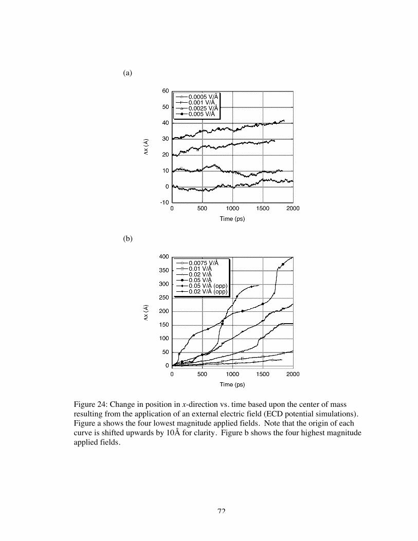
72
(a)
(b)
Figure 24: Change in position in x-direction vs. time based upon the center of massresulting from the application of an external electric field (ECD potential simulations).Figure a shows the four lowest magnitude applied fields. Note that the origin of eachcurve is shifted upwards by 10Å for clarity. Figure b shows the four highest magnitudeapplied fields.
73
IV.4 Discussion
In order to directly compare the results of the two simulation sets, the
translocation velocity has been obtained from the slope of the trajectories in Figures 22
and 24 and plotted against the electric field magnitude. The simulation translocation
velocity values are also compared to results from simulations of the ssDNA strand in bulk
water in Figure 25. The bulk water simulations were performed using the same
methodology as our previous bulk ssDNA simulations described in Chapter III and
elsewhere60.
Figure 25 reiterates the fact that the lower magnitude fields of the UFF
simulations resulted in very similar translocation velocities until the electric field became
large enough to overcome the resistance to motion created by the UFF potential
interactions. It appears that this resistance to motion is largely dependent on the ability of
the ssDNA strand to recruit a sufficient number of water molecules to surround it while
traversing the nanogate. The ECD simulations resulted in more linear response to applied
electric fields.
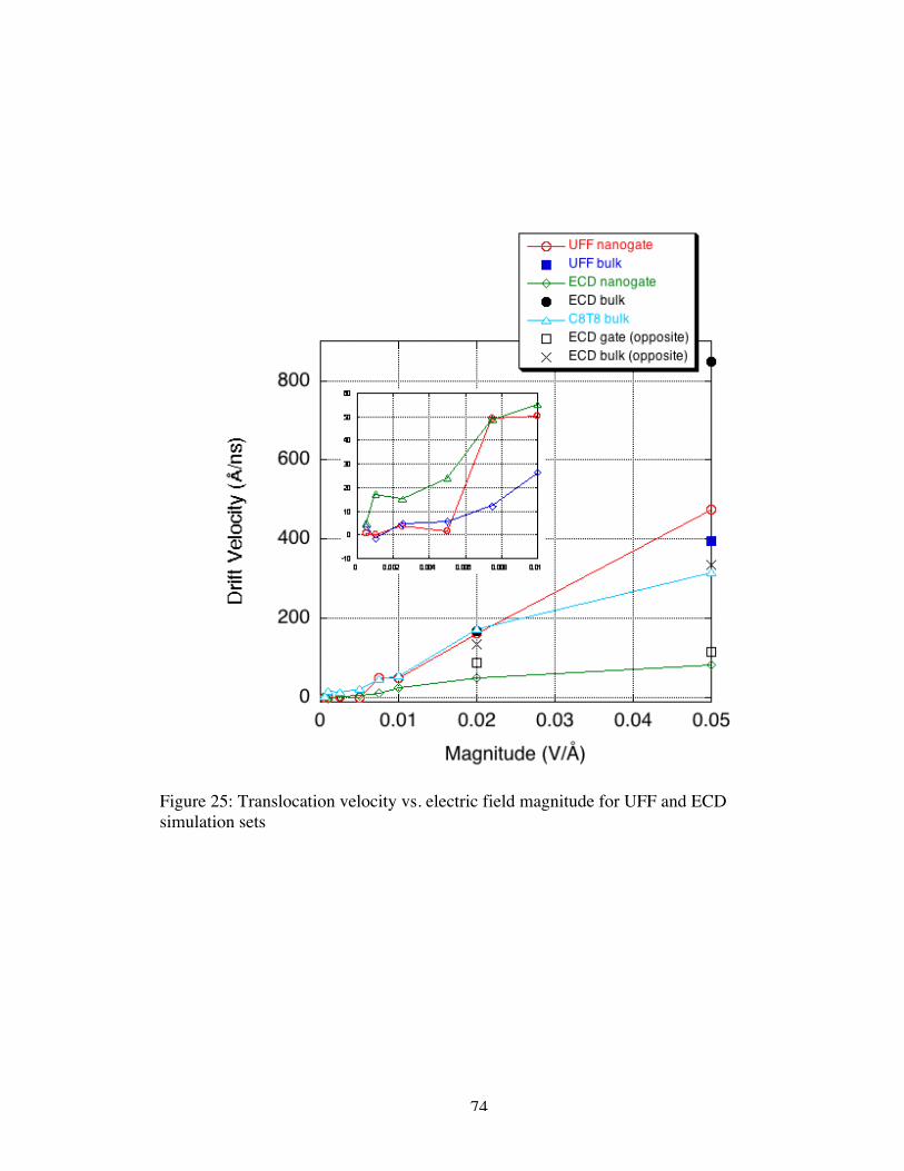
74
Figure 25: Translocation velocity vs. electric field magnitude for UFF and ECDsimulation sets
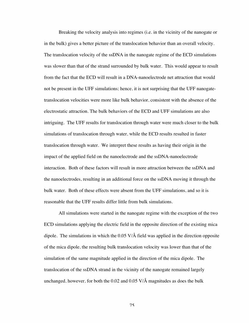
75
Breaking the velocity analysis into regimes (i.e. in the vicinity of the nanogate or
in the bulk) gives a better picture of the translocation behavior than an overall velocity.
The translocation velocity of the ssDNA in the nanogate regime of the ECD simulations
was slower than that of the strand surrounded by bulk water. This would appear to result
from the fact that the ECD will result in a DNA-nanoelectrode net attraction that would
not be present in the UFF simulations; hence, it is not surprising that the UFF nanogate-
translocation velocities were more like bulk behavior, consistent with the absence of the
electrostatic attraction. The bulk behaviors of the ECD and UFF simulations are also
intriguing. The UFF results for translocation through water were much closer to the bulk
simulations of translocation through water, while the ECD results resulted in faster
translocation through water. We interpret these results as having their origin in the
impact of the applied field on the nanoelectrode and the ssDNA-nanoelectrode
interaction. Both of these factors will result in more attraction between the ssDNA and
the nanoelectrodes, resulting in an additional force on the ssDNA moving it through the
bulk water. Both of these effects were absent from the UFF simulations, and so it is
reasonable that the UFF results differ little from bulk simulations.
All simulations were started in the nanogate regime with the exception of the two
ECD simulations applying the electric field in the opposite direction of the existing mica
dipole. The simulations in which the 0.05 V/Å field was applied in the direction opposite
of the mica dipole, the resulting bulk translocation velocity was lower than that of the
simulation of the same magnitude applied in the direction of the mica dipole. The
translocation of the ssDNA strand in the vicinity of the nanogate remained largely
unchanged, however, for both the 0.02 and 0.05 V/Å magnitudes as does the bulk
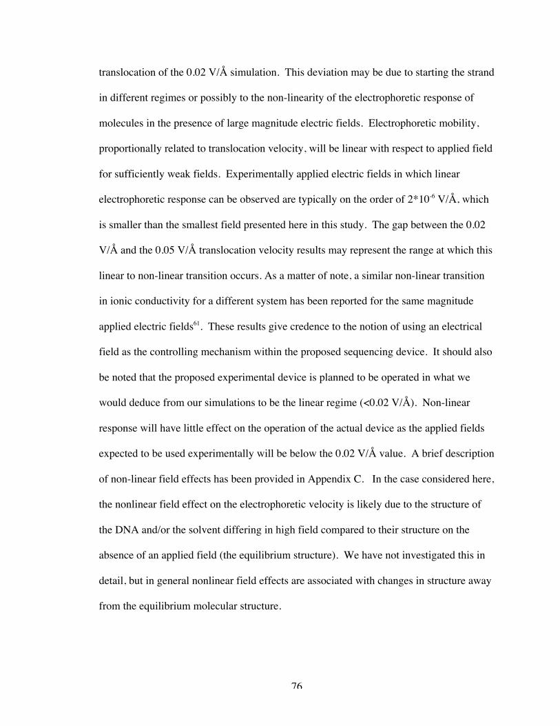
76
translocation of the 0.02 V/Å simulation. This deviation may be due to starting the strand
in different regimes or possibly to the non-linearity of the electrophoretic response of
molecules in the presence of large magnitude electric fields. Electrophoretic mobility,
proportionally related to translocation velocity, will be linear with respect to applied field
for sufficiently weak fields. Experimentally applied electric fields in which linear
electrophoretic response can be observed are typically on the order of 2*10-6 V/Å, which
is smaller than the smallest field presented here in this study. The gap between the 0.02
V/Å and the 0.05 V/Å translocation velocity results may represent the range at which this
linear to non-linear transition occurs. As a matter of note, a similar non-linear transition
in ionic conductivity for a different system has been reported for the same magnitude
applied electric fields61. These results give credence to the notion of using an electrical
field as the controlling mechanism within the proposed sequencing device. It should also
be noted that the proposed experimental device is planned to be operated in what we
would deduce from our simulations to be the linear regime (<0.02 V/Å). Non-linear
response will have little effect on the operation of the actual device as the applied fields
expected to be used experimentally will be below the 0.02 V/Å value. A brief description
of non-linear field effects has been provided in Appendix C. In the case considered here,
the nonlinear field effect on the electrophoretic velocity is likely due to the structure of
the DNA and/or the solvent differing in high field compared to their structure on the
absence of an applied field (the equilibrium structure). We have not investigated this in
detail, but in general nonlinear field effects are associated with changes in structure away
from the equilibrium molecular structure.
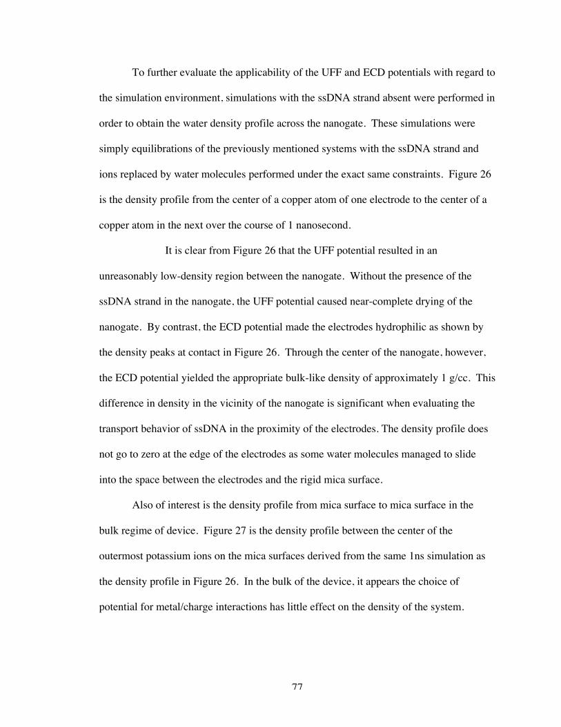
77
To further evaluate the applicability of the UFF and ECD potentials with regard to
the simulation environment, simulations with the ssDNA strand absent were performed in
order to obtain the water density profile across the nanogate. These simulations were
simply equilibrations of the previously mentioned systems with the ssDNA strand and
ions replaced by water molecules performed under the exact same constraints. Figure 26
is the density profile from the center of a copper atom of one electrode to the center of a
copper atom in the next over the course of 1 nanosecond.
It is clear from Figure 26 that the UFF potential resulted in an
unreasonably low-density region between the nanogate. Without the presence of the
ssDNA strand in the nanogate, the UFF potential caused near-complete drying of the
nanogate. By contrast, the ECD potential made the electrodes hydrophilic as shown by
the density peaks at contact in Figure 26. Through the center of the nanogate, however,
the ECD potential yielded the appropriate bulk-like density of approximately 1 g/cc. This
difference in density in the vicinity of the nanogate is significant when evaluating the
transport behavior of ssDNA in the proximity of the electrodes. The density profile does
not go to zero at the edge of the electrodes as some water molecules managed to slide
into the space between the electrodes and the rigid mica surface.
Also of interest is the density profile from mica surface to mica surface in the
bulk regime of device. Figure 27 is the density profile between the center of the
outermost potassium ions on the mica surfaces derived from the same 1ns simulation as
the density profile in Figure 26. In the bulk of the device, it appears the choice of
potential for metal/charge interactions has little effect on the density of the system.
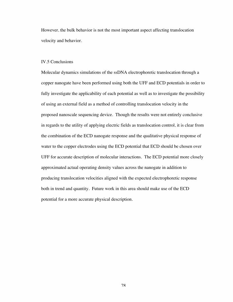
78
However, the bulk behavior is not the most important aspect affecting translocation
velocity and behavior.
IV.5 Conclusions
Molecular dynamics simulations of the ssDNA electrophoretic translocation through a
copper nanogate have been performed using both the UFF and ECD potentials in order to
fully investigate the applicability of each potential as well as to investigate the possibility
of using an external field as a method of controlling translocation velocity in the
proposed nanoscale sequencing device. Though the results were not entirely conclusive
in regards to the utility of applying electric fields as translocation control, it is clear from
the combination of the ECD nanogate response and the qualitative physical response of
water to the copper electrodes using the ECD potential that ECD should be chosen over
UFF for accurate description of molecular interactions. The ECD potential more closely
approximated actual operating density values across the nanogate in addition to
producing translocation velocities aligned with the expected electrophoretic response
both in trend and quantity. Future work in this area should make use of the ECD
potential for a more accurate physical description.
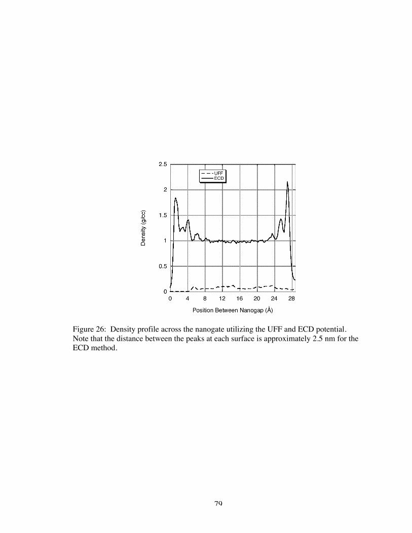
79
Figure 26: Density profile across the nanogate utilizing the UFF and ECD potential.Note that the distance between the peaks at each surface is approximately 2.5 nm for theECD method.
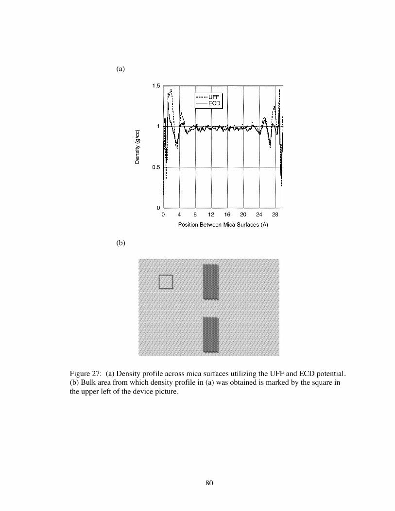
80
(a)
(b)
Figure 27: (a) Density profile across mica surfaces utilizing the UFF and ECD potential.(b) Bulk area from which density profile in (a) was obtained is marked by the square inthe upper left of the device picture.
81
CHAPTER V
ELECTROPHORESIS OF ssDNA THROUGH NANOELECTRODE GAPS: IMPACTOF GAP WIDTH
V.1 Introduction
In this study, through the use of molecular dynamics simulations, we attempt to address
one of the fundamental questions, namely, the physical behavior of the translocating
DNA in the sequencing device and its response to the basic device design variable, the
nano gap width (i.e., the nanoscopic distance between the two nano-electrodes).
Our previous simulations37 of the proposed sequencing device shown in Figure 1
focused on the effects of the applied electric field on the translocation velocity of the
ssDNA strand, in addition to the proper application of interaction potential. It was
concluded that use of an applied electric field would provide sufficient force to initiate
forward motion through the nanoscale gap, though the actual magnitude and shape of the
field necessary has yet to be determined as it is dependent on other variables such as
DNA strand length, solvent viscosity, and gap width. In the simulations presented in this
chapter, we examine the effect of changing the gap width on the translocation of ssDNA
through the nanoscale gap. We demonstrate that the gap width clearly has a significant
impact on the ability of the ssDNA strand to effectively translocate. In addition, our
simulations indicate a threshold value for which the ssDNA will enter and thread the gap
during the course of a molecular dynamics simulation. we will also present the modified-
Morse fit results for platinum to be applied in the ECD method.
82
V.2 Computational Method
V.2.A System Setup
Each simulation performed was of a nanoscale sequencing device consisting of two mica
plates separated by approximately 3 nm; the solvated DNA, counterions, and water are
enclosed between the plates. Each plate has dimensions of 20.7 nm x 14.4 nm. The
detection nodes were constructed of two platinum FCC lattices measuring approximately
2 nm x 5 nm x 3 nm. The separation distance of these nodes was measured from center
to center of the outermost platinum atoms. We considered values of 1.5, 1.75, 2.0, 2.25,
2.5, 2.75, 3.0, and 3.25 nm. These values are the nominal gap width. The effective gaps
are usually about 0.3 nm narrower than the nominal gaps because of the van der Waals
radius of the metal atoms determining the gap. The ssDNA strand used in the present
study consisted of sixteen nucleotides, eight consecutive cytosines followed by eight
consecutive thymines. The strand was solvated in water at a density of 1g/cc, and was
surrounded by 15 sodium ions in solution to make the total system charge-neutral. The
number of atoms in each of these simulations varied slightly but all eight simulations
were of approximately 138,000 atoms. The total dimension of the simulation box was
20.7 nm x 14.4 nm x 5.0 nm (including mica atoms). The simulations were periodic in
the x and y directions. The z direction was modeled by a slab geometry as described
before. These boundary conditions allow the DNA strand to continue movement across
boundaries in the x and y direction and reduces computational expenditure, since the 3-D
slab geometry technique for PPPM is less computationally demanding than using a 2-D
Ewald method33. Note that the mica surfaces were parallel to the x-y plane.
83
The ssDNA strand was positioned at the entrance of the gap between the
electrodes, which will be referred to here as the nanogate. The head ssDNA residue is
lined up with the nanogate such that the lead hydrogen atom on the backbone is exactly
even with the x-position of the first row of platinum atoms comprising the nanogate. This
positioning alleviated the need to examine ssDNA conformational effects on the transport
behavior. Experimentally, proper alignment of the ssDNA strand to ensure translocation
will have to be addressed, most likely through the use of nanofluidic transport to the
nanogate.
V.2.B Force Fields
The nucleic acids were described using the CHARMM27 all-hydrogen potential26, 27. The
sodium ions were represented by a potential developed by Beglov and Roux28, included
in the CHARMM potential. Water molecules were described by the rigid water model
known as TIP3P29 with which the CHARMM potential has been optimized. A more
rigorous water potential was unnecessary in comparison to the need for computational
efficiency for such a large system. The mica surfaces and the platinum nodes were
treated as rigid bodies in this set of simulations. As such, their non-electrostatic
interactions with other atoms were calculated by Lennard-Jones potential with parameters
determined by Lorentz-Berthelot mixing rules. The CLAYFF potential30 parameters were
used for mica, and the ECD methodology was used for the platinum atoms. Note that,
according to the experimental studies of Klein50 and the simulations of Leng and
Cummings51, 52, the fluidity of water confined between two mica surfaces is maintained
under extreme confinement (i.e., mica-to-mica distances of less than 1 nm); hence, we
84
expect that the water confined between the mica surfaces in our simulation (with mica-to-
mica distances of 3 nm) will exhibit fluidity similar to that of bulk water.
V.2.C ECD Platinum Parameters
As discussed in the previous chapter, the ECD method more accurately describes the
phenomena of varying charge density in response to Coulombic forces acting on the
metal by representing valence electrons with a diffuse negative Gaussian charge-density
distribution and representing the core electrons and the nuclei as fixed positive point
charges. This description of interactions is further supplemented by the addition of a
modified-Morse potential utilizing parameters fit from ab initio data.
In order to use the ECD method in these simulations, or for any simulation using
metal other than copper, we must first fit a modified-Morse potential,
€
U(r ) = −ε 1− 1− exp −A r − r *( )[ ]{ }2
(18)
to the difference between the ab initio and ECD Coulombic interactions. In Equation
(18), U is the potential energy, r is the distance from the atom center, and ε, A and r* are
the adjustable parameters,.
Density functional theory (DFT) data for the interaction of a water molecule with
a platinum (111) surface was obtained from Meng and coworkers62. The TIP3P water
geometry and charges were used for the ECD calculations and simulations. ECD
Coulombic interactions were determined from a sample surface of 64 platinum atoms in a
FCC (111) lattice consisting of four layers of platinum atoms with a vacuum region of
approximately 13 Å, in order to mimic the DFT study setup. The water molecule was
held directly over a top site (i.e. directly above a platinum atom) because this position has

85
been shown to be the most favorable adsorption site. Ideally, the water molecule lies
almost flat on the surface with its polar axis making an angle (θ) of 13º to 14º at
approximately 2.43 Å above the top site. The energy was calculated as the water
molecule was moved in a variety of positions. The first set of energies shown in Figure
28a was determined as the molecule was moved vertically from the top site maintaining
the 13-14º angle. The second set shown in Figure 28b was determined as the molecule
was held at 2.43 Å above the top site, and the surface-molecule angle was varied.
Negative surface angle indicates the molecules hydrogen atoms were facing the platinum
surface. Positive surface angles indicate the hydrogen atoms were facing the vacuum
region.
The fit was determined using Excel solver to perform weighted least squares
regression. The fit was weighted to the ideal distance above the surface and ideal angle
with the surface because of their importance in description. Table 1 gives the values we
obtained and used in the above-described simulations.
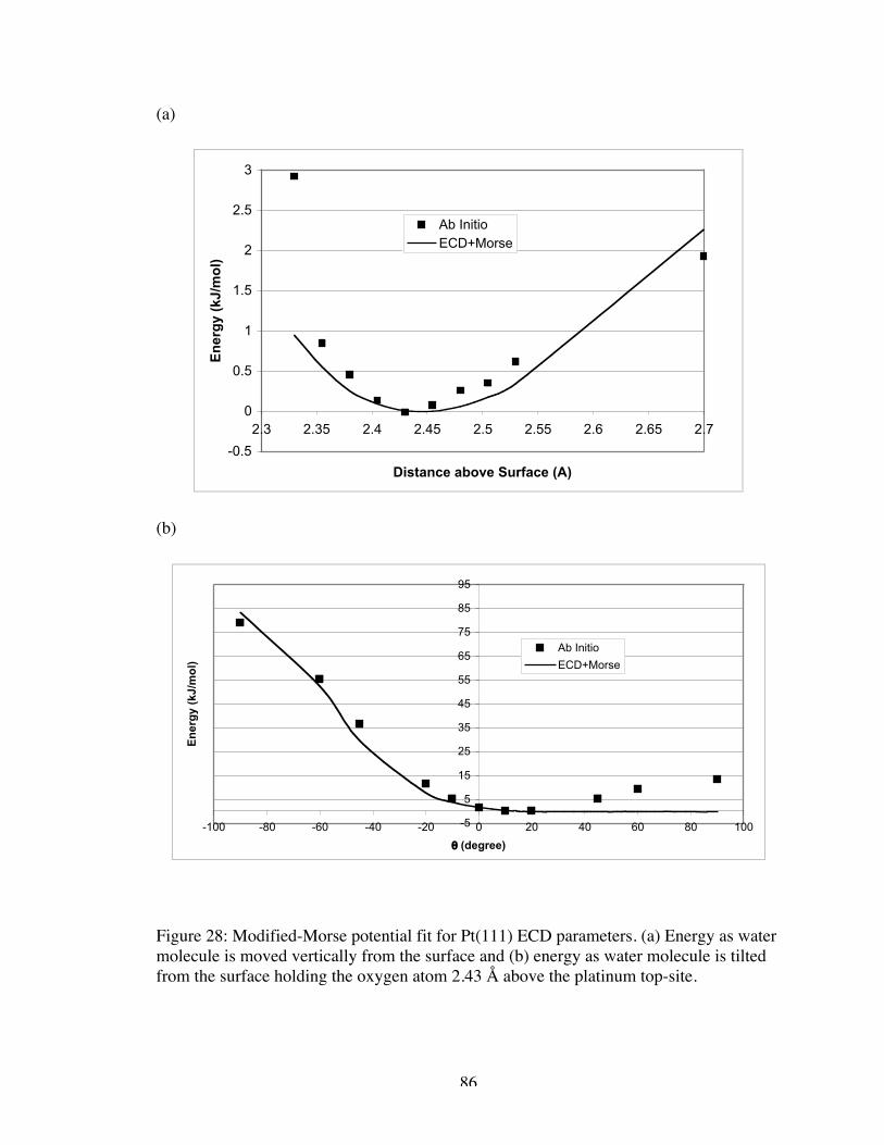
86
(a)
-0.5
0
0.5
1
1.5
2
2.5
3
2.3 2.35 2.4 2.45 2.5 2.55 2.6 2.65 2.7
Distance above Surface (A)
Ener
gy (k
J/m
ol)
Ab InitioECD+Morse
(b)
-5
5
15
25
35
45
55
65
75
85
95
-100 -80 -60 -40 -20 0 20 40 60 80 100θ (degree)
Ener
gy (k
J/m
ol)
Ab InitioECD+Morse
Figure 28: Modified-Morse potential fit for Pt(111) ECD parameters. (a) Energy as watermolecule is moved vertically from the surface and (b) energy as water molecule is tiltedfrom the surface holding the oxygen atom 2.43 Å above the platinum top-site.

87
Table 1: Interaction parameters for use with modified-Morse potential for Pt (111).
O H
ε, kJ/mol 0.831 1.621
A, Å-1 2.000 2.320
r*, Å 3.073 2.768
88
Additionally, the ECD methodology involves two additional parameters, qc, core
charge, and γ, an inverse-width parameter, to characterize the polarization behavior of the
metal. In the ECD method, the metal ions are represented as positively charged spheres,
whose charge has the same magnitude as the valence electron charge per atom; hence, for
platinum, the charge on the core of the platinum ion qc is 1.0 |e|. The ECD method
assigned a Gaussian electron charge distribution to each atom to represent the valence
electrons. The inverse of the width of this distribution, γ, for platinum is obtained by
fitting to the ab initio calculations to be 0.751 Å-1. The ECD parameters for platinum
have not previously been published and represent a new finding in this work. In the ECD
method42, the magnitude of the charge associated with each metal ion fluctuates in
response to interactions with charges outside the surface (e.g., partial charges in the water
molecule) subject to the overall constraint of the total charge on the metallic
nanostructure (zero in our case). In this way, the effect of valence electron mobility
within the metallic nanostructure is taken into account; in a macroscopic system, this
same mobility is taken into account via image charges.
V.2.D Simulation Details
The classical molecular dynamics simulations were performed using the modified version
of the LAMMPS (Large-scale Atomic/Molecular Massively Parallel Simulator)24, 25
simulation package as described in the previous chapter.
All simulations began with an equilibration period of 430 ps. Simulations were
performed using the NVT ensemble at 300K with a Nosé-Hoover thermostat46. Time
integration was performed using the velocity-Verlet algorithm with a 2 fs timestep2.
89
Bonds involving hydrogen atoms were constrained using the SHAKE algorithm48. The
particle-particle particle-mesh (PPPM) solver was used to compute long-range
Coulombic interactions32.
After the equilibration period, the simulations were subjected to an applied
uniform electric field of 0.02 V/Å, corresponding to an effective transmembrane voltage
drop of 40 mV, and a production run of 1 ns was performed. This uniform field was
applied in the x-direction in order to force the ssDNA to translocate through the
nanoscale gap. For the sake of computational expense, a uniform field was used without
the additional perpendicular holding pulse as proposed in the original device design.
Note that the results shown below are of single trajectories. While ensemble averages
would be useful in generalizing behavior, we believe that the results presented still
properly illustrate the transport phenomena, and in particular, demonstrate clearly the
impact of the gate width on translocation behavior.
V.3 Results
The results of the platinum nanogate gap width on the translocation of the ssDNA strand
has been evaluated here through examination of the trajectories in the ssDNA molecule’s
center of mass along the x-direction as well as the molecule’s end-to-end distance.
The center of mass was used as the point of reference for the molecule’s motion
in this study. Figure 29 shows the change in center of mass in the x-direction versus time.
From this slope of each of these lines, we determined the translocation velocity.
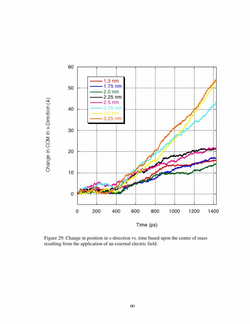
90
Figure 29: Change in position in x-direction vs. time based upon the center of massresulting from the application of an external electric field.
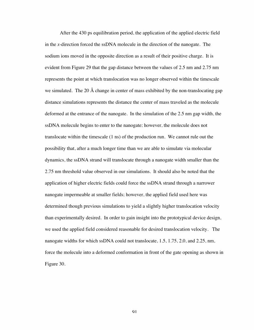
91
After the 430 ps equilibration period, the application of the applied electric field
in the x-direction forced the ssDNA molecule in the direction of the nanogate. The
sodium ions moved in the opposite direction as a result of their positive charge. It is
evident from Figure 29 that the gap distance between the values of 2.5 nm and 2.75 nm
represents the point at which translocation was no longer observed within the timescale
we simulated. The 20 Å change in center of mass exhibited by the non-translocating gap
distance simulations represents the distance the center of mass traveled as the molecule
deformed at the entrance of the nanogate. In the simulation of the 2.5 nm gap width, the
ssDNA molecule begins to enter to the nanogate; however, the molecule does not
translocate within the timescale (1 ns) of the production run. We cannot rule out the
possibility that, after a much longer time than we are able to simulate via molecular
dynamics, the ssDNA strand will translocate through a nanogate width smaller than the
2.75 nm threshold value observed in our simulations. It should also be noted that the
application of higher electric fields could force the ssDNA strand through a narrower
nanogate impermeable at smaller fields; however, the applied field used here was
determined though previous simulations to yield a slightly higher translocation velocity
than experimentally desired. In order to gain insight into the prototypical device design,
we used the applied field considered reasonable for desired translocation velocity. The
nanogate widths for which ssDNA could not translocate, 1.5, 1.75, 2.0, and 2.25, nm,
force the molecule into a deformed conformation in front of the gate opening as shown in
Figure 30.
92
Figure 30: Snapshot of 1.75 nm gate width simulation after 1 ns production run (waternot shown for clarity).
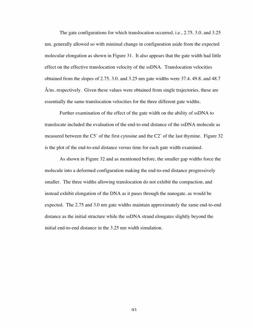
93
The gate configurations for which translocation occurred, i.e., 2.75, 3.0, and 3.25
nm, generally allowed so with minimal change in configuration aside from the expected
molecular elongation as shown in Figure 31. It also appears that the gate width had little
effect on the effective translocation velocity of the ssDNA. Translocation velocities
obtained from the slopes of 2.75, 3.0, and 3.25 nm gate widths were 37.4, 49.8, and 48.7
Å/ns, respectively. Given these values were obtained from single trajectories, these are
essentially the same translocation velocities for the three different gate widths.
Further examination of the effect of the gate width on the ability of ssDNA to
translocate included the evaluation of the end-to-end distance of the ssDNA molecule as
measured between the C5’ of the first cytosine and the C2’ of the last thymine. Figure 32
is the plot of the end-to-end distance versus time for each gate width examined.
As shown in Figure 32 and as mentioned before, the smaller gap widths force the
molecule into a deformed configuration making the end-to-end distance progressively
smaller. The three widths allowing translocation do not exhibit the compaction, and
instead exhibit elongation of the DNA as it pases through the nanogate, as would be
expected. The 2.75 and 3.0 nm gate widths maintain approximately the same end-to-end
distance as the initial structure while the ssDNA strand elongates slightly beyond the
initial end-to-end distance in the 3.25 nm width simulation.
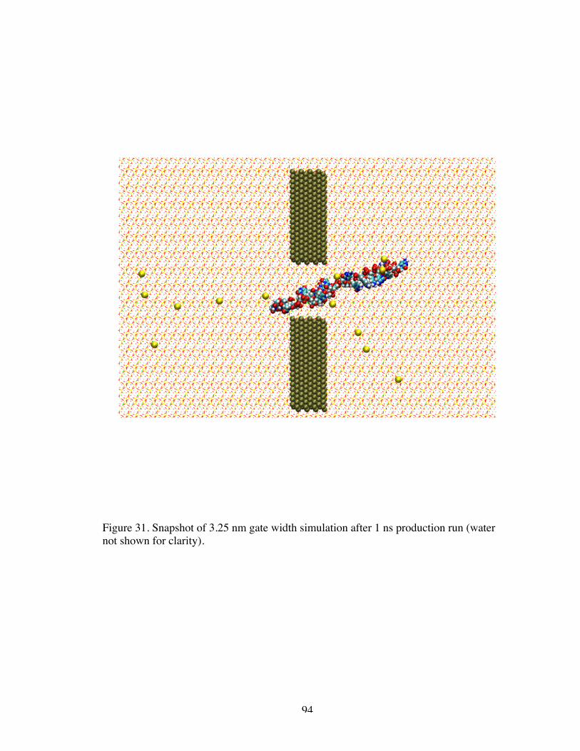
94
Figure 31. Snapshot of 3.25 nm gate width simulation after 1 ns production run (waternot shown for clarity).
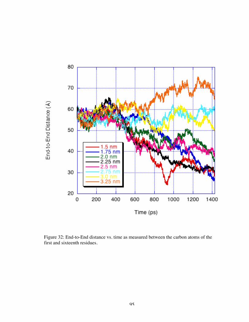
95
Figure 32: End-to-End distance vs. time as measured between the carbon atoms of thefirst and sixteenth residues.
96
Figure 32 serves as an explanation why the threshold gap width found in this
work is large when compared with other previous studies of synthetic nanopore
translocation63. Heng, et al. determined that ssDNA can permeate Si3N4 pores less than 1
nm in diameter under the influence of low electric fields. Single-stranded DNA, as
opposed to the typical double-stranded DNA molecule, allows for more flexibility in
translocation, enabling the molecule to readily translocate in smaller pores. However, in
our simulations, we find that the ssDNA would fold rather than translocate and
experience significant deformation thus increasing its effective characteristic dimension.
We suggest that the folding is caused by the strong ssDNA-electrode attraction induced
by electrostatic interactions with the metal modeled by ECD. Additionally, in the system
used by Heng et al., the double-conical nanopore limits the molecular deformation at the
entrance to the narrowest portion of the pore. The pore length examined by Heng et al.
was much larger than we have simulated (10 nm as opposed to 2 nm) with an advantage
of 1 nm of the helix being threaded within the pore at the start of the simulation, whereas
in our simulation the ssDNA begins outside the pore. Also of note is the 8kT energetic
barrier to translocation of ssDNA through an α-hemolysin protein pore discovered by
Henrickson et al.64. This suggests that a minimum amount of applied field is necessary
solely to enter the nanopore. This energy may be quite different than that required in the
system devised by Heng et al., precluding the entrance to the rigid metallic nanopore
used in our simulation in some cases.
For the purpose of clarifying visually what is occurring through the application of
the ECD methodology, we have presented the simulation trajectory in Figure 33 of the
3.25 nm gate width visualizing the change in charge. Red represents positively charged

97
atoms, and blue represents negatively charged atoms. We can see the application of the
external potential tends to charge the electrodes in a positive to negative fashion from left
to right. The backbone of the DNA strand is negatively charged and hence attracted to
the electrodes. In our previous applied field study, we determined that the ssDNA strand
travels rapidly through the bulk due to this attraction to the nanogate. Additionally, we
can see that the application of ECD to describe the electrostatic potentials does indeed
allow for charge density variation in response to the environment in the vicinity of the
metal atoms.
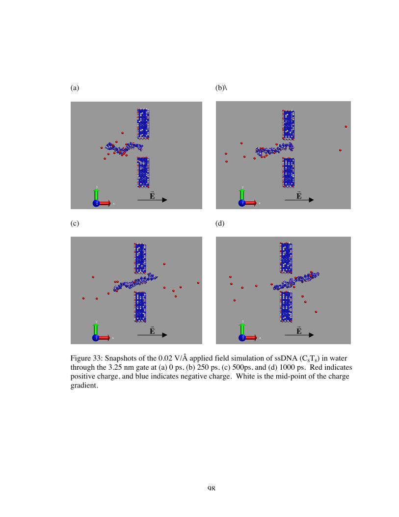
98
(a) (b)\
(c) (d)
Figure 33: Snapshots of the 0.02 V/Å applied field simulation of ssDNA (C8T8) in waterthrough the 3.25 nm gate at (a) 0 ps, (b) 250 ps, (c) 500ps, and (d) 1000 ps. Red indicatespositive charge, and blue indicates negative charge. White is the mid-point of the chargegradient.
€
r E
€
r E
€
r E
€
r E
99
V.4 Conclusions
Molecular dynamics simulations of the ssDNA electrophoretic translocation through a
platinum nanogate have been performed in order to fully investigate the gate width
design variable. As expected, there exists a specific gate width for which the ssDNA
strand will no longer translocate over the time scale of the simulation. For the applied
field of 0.02 V/Å, the strand will not translocate through a gate width smaller than
approximately 2.5 nm. The application of a stronger electrophoretic driving field might
be able to force the strand through a smaller gate opening over the time scale simulated;
however, we chose to use an experimentally relevant magnitude field in the simulation to
yield desired translocation velocities as determined by our previous studies. Once the
gate is large enough to allow translocation, the actual size of the gate appears to be
irrelevant. The translocation velocity appears to be largely insensitive to the gate width
beyond the minimum. However, we expect that if the gap is large enough to allow
folding within the gap, this may impact translocation velocity. The translocation
velocities observed for the translocating gate widths are roughly the same as the
approximately 40 Å/ns translocation velocity we infer from simulations for a similar
ssDNA molecule in bulk water60 at the same applied field, which in turn is consistent
with experimental results for translocation in bulk. The threshold value we have found
in our simulations is larger than previously examined systems; however, there are many
differences in the simulations to consider including the ssDNA, the initial conditions,
pore geometry and nature of the pore, so that comparisons are difficult to make.
100
CHAPTER VI
ELECTROPHORESIS OF ssDNA THROUGH NANOELECTRODE GAPS: IMPACTOF SAMPLE LENGTH
VI.1 Introduction
This chapter presents the results of a set of simulations designed to examine the effect the
DNA sample length has upon translocation velocity. Using the same simulation setup as
previous simulations, we have introduced seven different length ssDNA strands varying
from 4 to 48 nucleotides in length. Ideally, we would be able to compare finite length
strand behavior to infinite (within the scale of simulation) length behavior; however, we
are limited in scope by the size of our simulated device and the electrostatic cutoff value
as well as by computational resources. We will present velocity results for translocating
strand lengths as well as explanation for non-translocating molecules.
VI.2 Computational Methods
Each simulation performed was of a nanoscale sequencing device consisting of two mica
plates separated by approximately 3 nm; the solvated DNA, counterions, and water are
enclosed between the plates. Each plate has dimensions of 20.7 nm x 14.4 nm. The
detection nodes were constructed of two platinum FCC lattices measuring approximately
2 nm x 5 nm x 3 nm. The separation distance of these nodes was measured from center
to center of the outermost platinum atoms. We used a constant value of 3.0 nm. This
value is a the nominal gap width as the effective gaps are usually about 0.3 nm narrower
101
than the nominal widths because of the van der Waals radius of the metal atoms
confining the gap.
The ssDNA strand used in the present study consisted of a varying number of
nucleotides solvated in water at a density of 1g/cc. The strands were comprised of a
repeating sequence of cytosine, thymine, adenine, and guanine (CTAG). We evaluated
seven different strand lengths denoted as CTAG, 2CTAG, 4CTAG, 6CTAG, 8CTAG,
10CTAG, and 12CTAG. The number in the abbreviation refers to the number of times
the base CTAG is repeated (i.e., 4CTAG refers to the nucleotide sequence
CTAGCTAGCTAGCTAG). The ssDNA strand was surrounded by an appropriate
number of sodium ions to make the total system charge-neutral (3 for CTAG, 7 for
2CTAG, 15 for 4CTAG, etc.). The number of atoms in each of these simulations varied
slightly but all seven simulations were of approximately 138,000 atoms. The total
dimension of the simulation box was 20.7 nm x 14.4 nm x 5.0 nm (including mica
atoms). The simulations were periodic in the x and y directions and fixed in the z
direction. Note that the mica surfaces were parallel to the x-y plane.
The ssDNA strand was positioned at the entrance of the gap between the
electrodes, which will be referred to here as the nanogate. The head ssDNA residue is
lined up with the nanogate such that the lead hydrogen atom on the backbone is exactly
even with the x-position of the first row of platinum atoms comprising the nanogate. This
positioning alleviated the need to examine ssDNA conformational effects on the transport
behavior. Experimentally, proper alignment of the ssDNA strand to ensure translocation
will have to be addressed, most likely through the use of nanofluidic transport to the
nanogate. We will present evidence to this effect shortly.
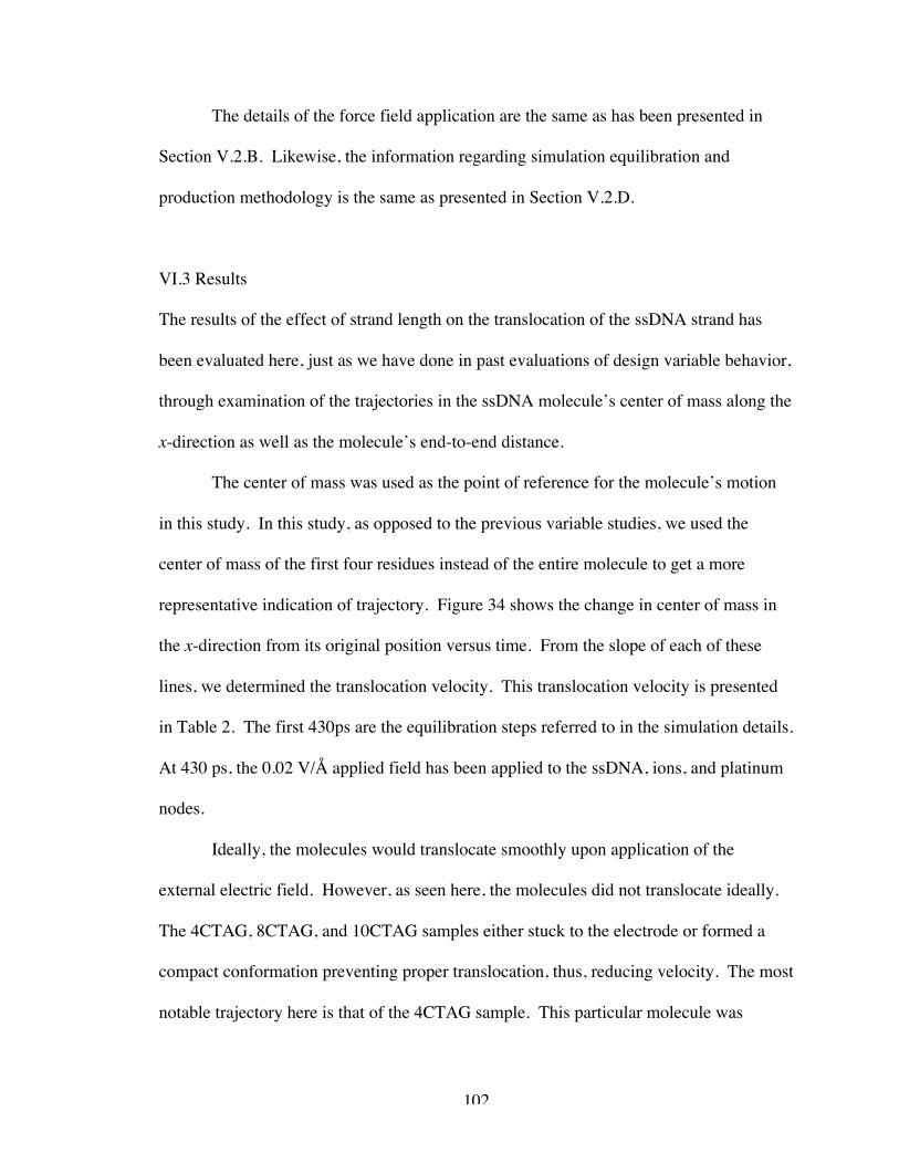
102
The details of the force field application are the same as has been presented in
Section V.2.B. Likewise, the information regarding simulation equilibration and
production methodology is the same as presented in Section V.2.D.
VI.3 Results
The results of the effect of strand length on the translocation of the ssDNA strand has
been evaluated here, just as we have done in past evaluations of design variable behavior,
through examination of the trajectories in the ssDNA molecule’s center of mass along the
x-direction as well as the molecule’s end-to-end distance.
The center of mass was used as the point of reference for the molecule’s motion
in this study. In this study, as opposed to the previous variable studies, we used the
center of mass of the first four residues instead of the entire molecule to get a more
representative indication of trajectory. Figure 34 shows the change in center of mass in
the x-direction from its original position versus time. From the slope of each of these
lines, we determined the translocation velocity. This translocation velocity is presented
in Table 2. The first 430ps are the equilibration steps referred to in the simulation details.
At 430 ps, the 0.02 V/Å applied field has been applied to the ssDNA, ions, and platinum
nodes.
Ideally, the molecules would translocate smoothly upon application of the
external electric field. However, as seen here, the molecules did not translocate ideally.
The 4CTAG, 8CTAG, and 10CTAG samples either stuck to the electrode or formed a
compact conformation preventing proper translocation, thus, reducing velocity. The most
notable trajectory here is that of the 4CTAG sample. This particular molecule was

103
particularly attracted to the metal electrodes. This attraction prevented linear
translocation. The remaining part of the strand was forced through the nanogap and a
bent conformation within the electrodes formed. Figure 35 illustrates through snapshots
the molecular deformation as described for the 4CTAG sample. If the molecules had
translocated ideally, we would have seen that the translocation velocity is relatively the
same regardless of the chain length.
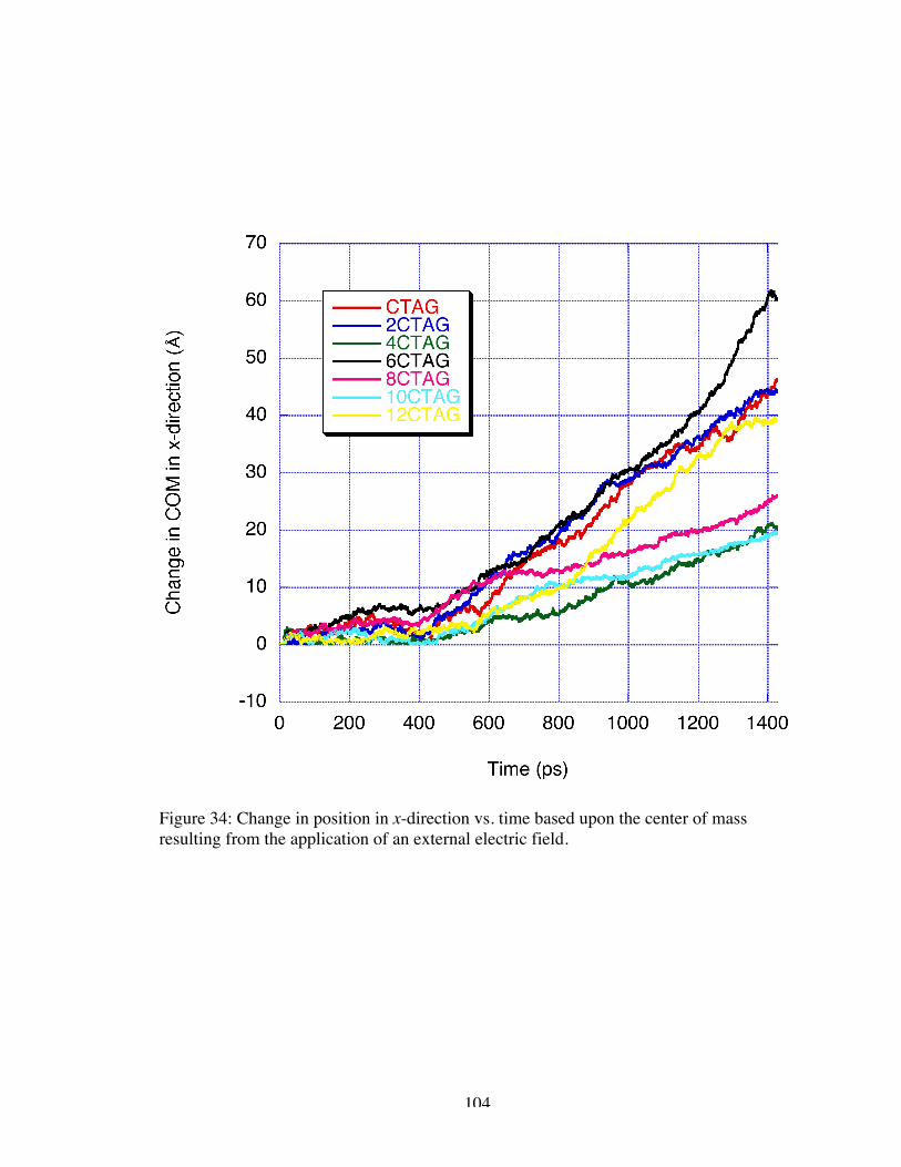
104
Figure 34: Change in position in x-direction vs. time based upon the center of massresulting from the application of an external electric field.
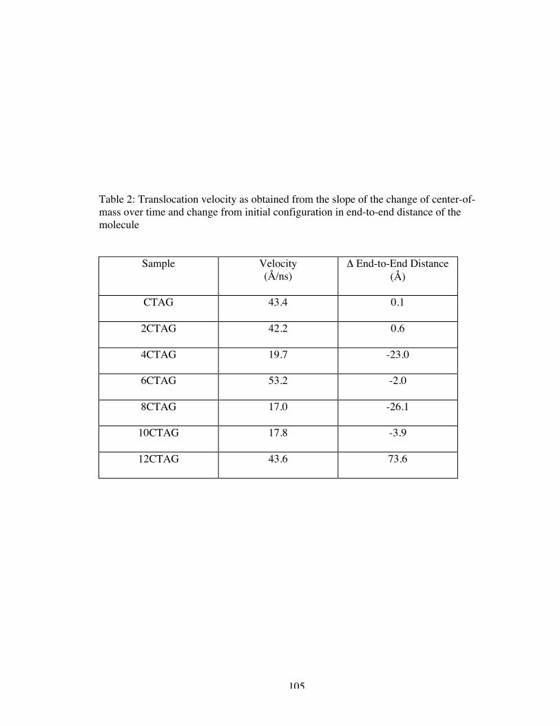
105
Table 2: Translocation velocity as obtained from the slope of the change of center-of-mass over time and change from initial configuration in end-to-end distance of themolecule
Sample Velocity(Å/ns)
Δ End-to-End Distance(Å)
CTAG 43.4 0.1
2CTAG 42.2 0.6
4CTAG 19.7 -23.0
6CTAG 53.2 -2.0
8CTAG 17.0 -26.1
10CTAG 17.8 -3.9
12CTAG 43.6 73.6
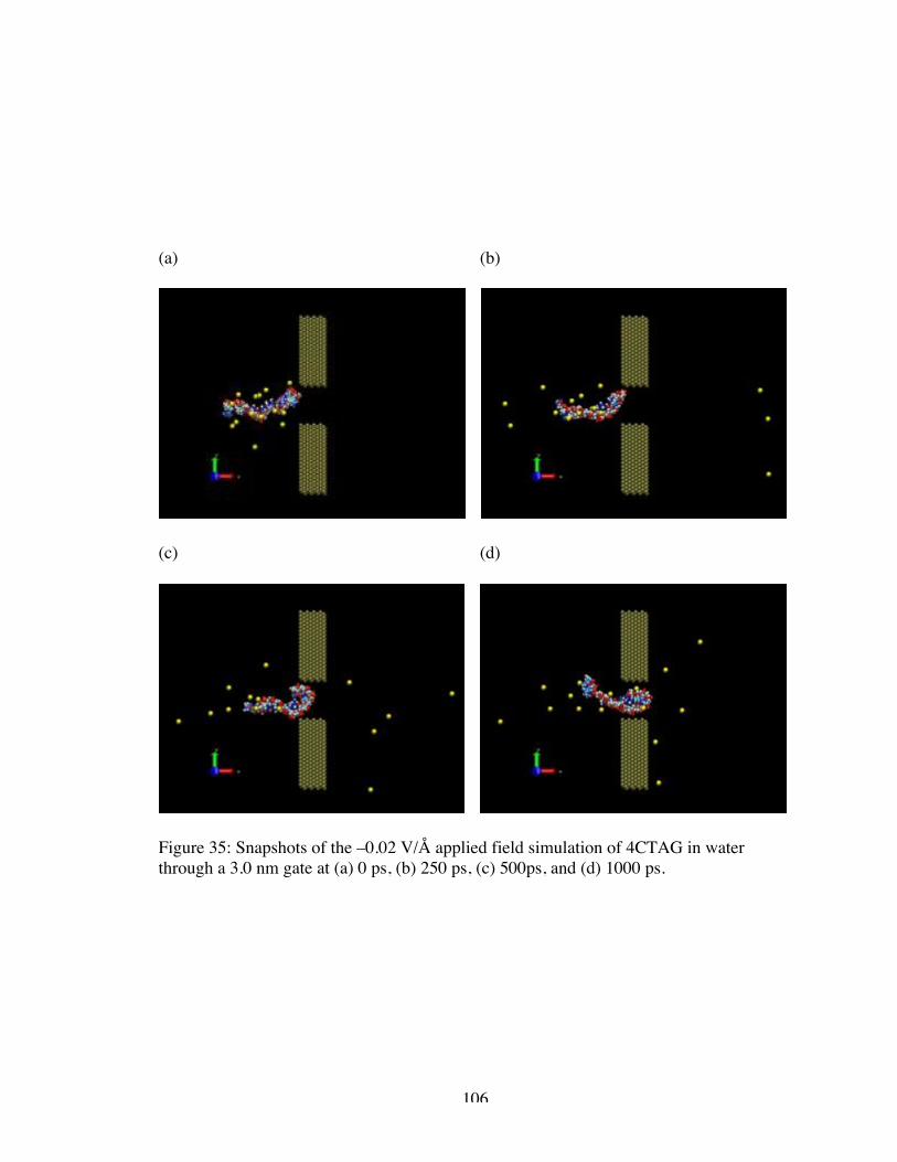
106
(a) (b)
(c) (d)
Figure 35: Snapshots of the –0.02 V/Å applied field simulation of 4CTAG in waterthrough a 3.0 nm gate at (a) 0 ps, (b) 250 ps, (c) 500ps, and (d) 1000 ps.
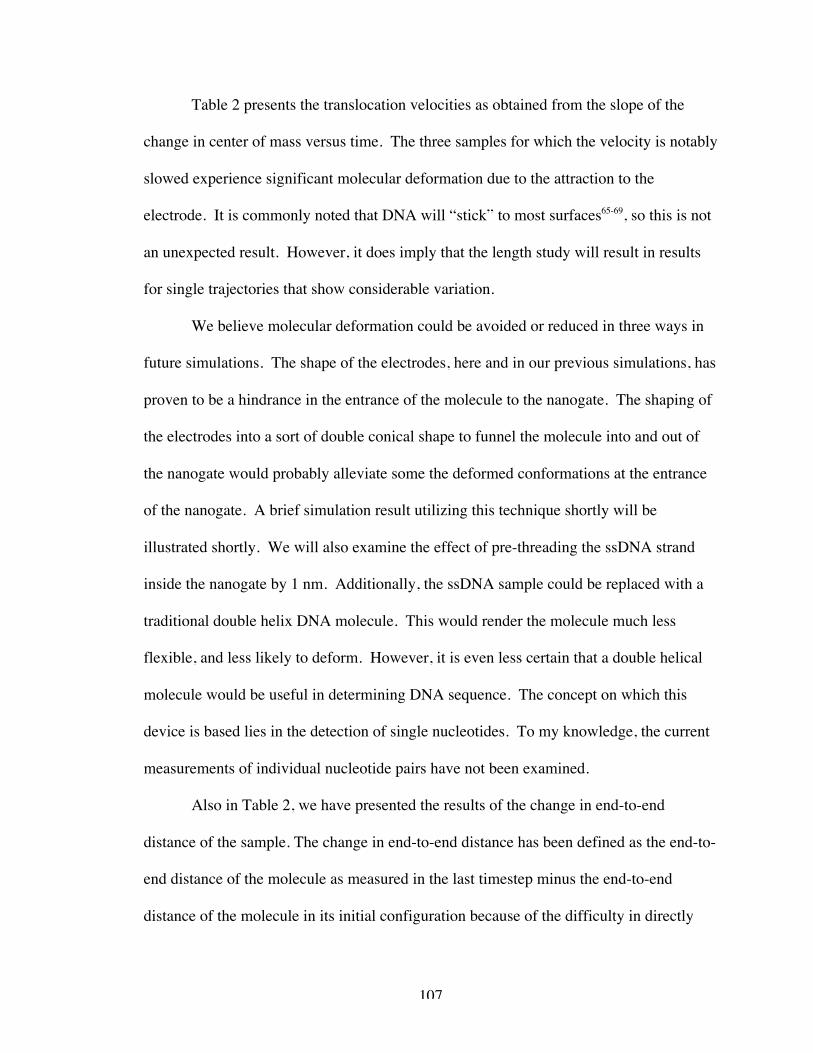
107
Table 2 presents the translocation velocities as obtained from the slope of the
change in center of mass versus time. The three samples for which the velocity is notably
slowed experience significant molecular deformation due to the attraction to the
electrode. It is commonly noted that DNA will “stick” to most surfaces65-69, so this is not
an unexpected result. However, it does imply that the length study will result in results
for single trajectories that show considerable variation.
We believe molecular deformation could be avoided or reduced in three ways in
future simulations. The shape of the electrodes, here and in our previous simulations, has
proven to be a hindrance in the entrance of the molecule to the nanogate. The shaping of
the electrodes into a sort of double conical shape to funnel the molecule into and out of
the nanogate would probably alleviate some the deformed conformations at the entrance
of the nanogate. A brief simulation result utilizing this technique shortly will be
illustrated shortly. We will also examine the effect of pre-threading the ssDNA strand
inside the nanogate by 1 nm. Additionally, the ssDNA sample could be replaced with a
traditional double helix DNA molecule. This would render the molecule much less
flexible, and less likely to deform. However, it is even less certain that a double helical
molecule would be useful in determining DNA sequence. The concept on which this
device is based lies in the detection of single nucleotides. To my knowledge, the current
measurements of individual nucleotide pairs have not been examined.
Also in Table 2, we have presented the results of the change in end-to-end
distance of the sample. The change in end-to-end distance has been defined as the end-to-
end distance of the molecule as measured in the last timestep minus the end-to-end
distance of the molecule in its initial configuration because of the difficulty in directly
108
comparing end-to-end distances of molecules of different initial lengths. End-to-end
distances were measured from C5’ atom of the first cytosine to the C2’ atom of the last
guanine. Ideal translocation would yield an elongated molecule as evidenced by portions
of the 12CTAG sample.
The negative values for end-to-end distance represent the compacting of the
molecule from it initial position. These generally correspond to the molecules with
slower translocation velocities. The two smallest samples had very little change in the
length of the molecule over the course of the nanosecond simulation.
VI.4 Shaped nanogate effects on translocation
VI.4.A System Setup and Simulation Details
This simulation used the same mica containment device as mentioned in Section VI.2.
We chose to evaluate the 4CTAG sample as previously defined due to its significant
deformation. The platinum electrodes were defined as has been done before for synthetic
nanopores63 as “double-conical” nanopores. Due to the confinement by the mica
surfaces, the platinum electrodes do not technically form a conical shape; however, the
shaping of the pore inside the device corresponds to this terminology. The platinum
atoms form a shape with a diameter of
€
d(x) = do + x tanγ (19)
where the center of the pore and narrowest point is x = 0, do is the diameter of the pore at
z = 0, and γ is the conical angle chosen here to be 45°. We chose do to be 2.5 nm here.
The pore is 5 nm long in the x-direction, 5 nm wide in the y-direction, and 3 nm thick in
109
the z-direction. The 4CTAG sample was threaded 1 nm inside the pore as measured from
the first platinum atom encountered in the x-direction.
We used the exact same potentials and simulation techniques as described in
Sections V.2.B and V.2.D.
VI.4.B Results
The addition of a shaped nanopore, at least as can be surmised from a single trajectory,
did little to alleviate the molecular deformation of the 4CTAG sample. Figure 36
illustrates through snapshots the compacting of the molecule into a deformed
conformation. The head groups appear to make progress through the nanogate; however,
the first cytosine group is attracted to one node while the tail guanine residue is attracted
to the opposite node.
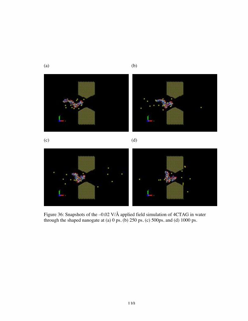
110
(a) (b)
(c) (d)
Figure 36: Snapshots of the –0.02 V/Å applied field simulation of 4CTAG in waterthrough the shaped nanogate at (a) 0 ps, (b) 250 ps, (c) 500ps, and (d) 1000 ps.
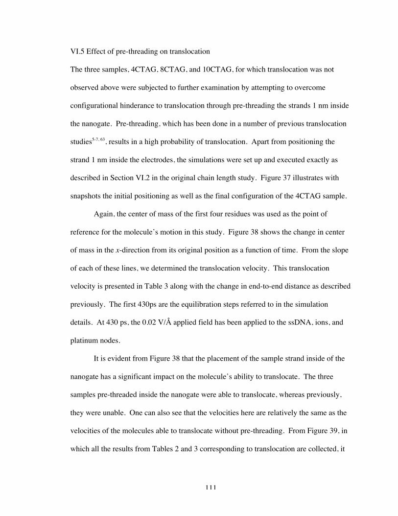
111
VI.5 Effect of pre-threading on translocation
The three samples, 4CTAG, 8CTAG, and 10CTAG, for which translocation was not
observed above were subjected to further examination by attempting to overcome
configurational hinderance to translocation through pre-threading the strands 1 nm inside
the nanogate. Pre-threading, which has been done in a number of previous translocation
studies5-7, 63, results in a high probability of translocation. Apart from positioning the
strand 1 nm inside the electrodes, the simulations were set up and executed exactly as
described in Section VI.2 in the original chain length study. Figure 37 illustrates with
snapshots the initial positioning as well as the final configuration of the 4CTAG sample.
Again, the center of mass of the first four residues was used as the point of
reference for the molecule’s motion in this study. Figure 38 shows the change in center
of mass in the x-direction from its original position as a function of time. From the slope
of each of these lines, we determined the translocation velocity. This translocation
velocity is presented in Table 3 along with the change in end-to-end distance as described
previously. The first 430ps are the equilibration steps referred to in the simulation
details. At 430 ps, the 0.02 V/Å applied field has been applied to the ssDNA, ions, and
platinum nodes.
It is evident from Figure 38 that the placement of the sample strand inside of the
nanogate has a significant impact on the molecule’s ability to translocate. The three
samples pre-threaded inside the nanogate were able to translocate, whereas previously,
they were unable. One can also see that the velocities here are relatively the same as the
velocities of the molecules able to translocate without pre-threading. From Figure 39, in
which all the results from Tables 2 and 3 corresponding to translocation are collected, it
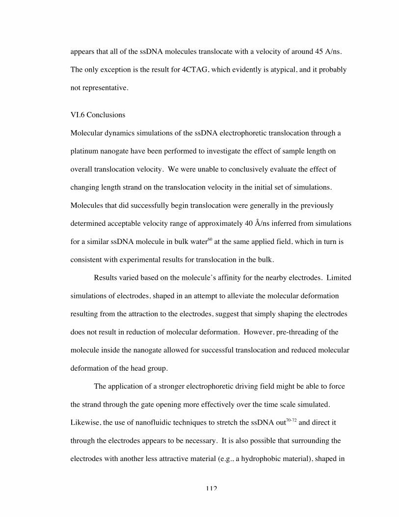
112
appears that all of the ssDNA molecules translocate with a velocity of around 45 A/ns.
The only exception is the result for 4CTAG, which evidently is atypical, and it probably
not representative.
VI.6 Conclusions
Molecular dynamics simulations of the ssDNA electrophoretic translocation through a
platinum nanogate have been performed to investigate the effect of sample length on
overall translocation velocity. We were unable to conclusively evaluate the effect of
changing length strand on the translocation velocity in the initial set of simulations.
Molecules that did successfully begin translocation were generally in the previously
determined acceptable velocity range of approximately 40 Å/ns inferred from simulations
for a similar ssDNA molecule in bulk water60 at the same applied field, which in turn is
consistent with experimental results for translocation in the bulk.
Results varied based on the molecule’s affinity for the nearby electrodes. Limited
simulations of electrodes, shaped in an attempt to alleviate the molecular deformation
resulting from the attraction to the electrodes, suggest that simply shaping the electrodes
does not result in reduction of molecular deformation. However, pre-threading of the
molecule inside the nanogate allowed for successful translocation and reduced molecular
deformation of the head group.
The application of a stronger electrophoretic driving field might be able to force
the strand through the gate opening more effectively over the time scale simulated.
Likewise, the use of nanofluidic techniques to stretch the ssDNA out70-72 and direct it
through the electrodes appears to be necessary. It is also possible that surrounding the
electrodes with another less attractive material (e.g., a hydrophobic material), shaped in

113
order to channel the ssDNA into the nanoelectrode gap, may result in reduced molecular
deformation.
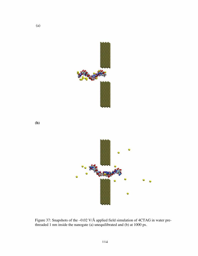
114
(a)
(b)
Figure 37: Snapshots of the –0.02 V/Å applied field simulation of 4CTAG in water pre-threaded 1 nm inside the nanogate (a) unequilibrated and (b) at 1000 ps.
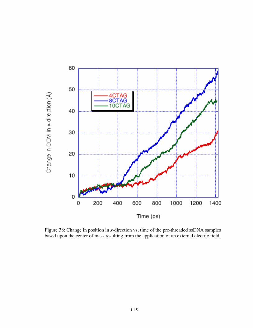
115
Figure 38: Change in position in x-direction vs. time of the pre-threaded ssDNA samplesbased upon the center of mass resulting from the application of an external electric field.
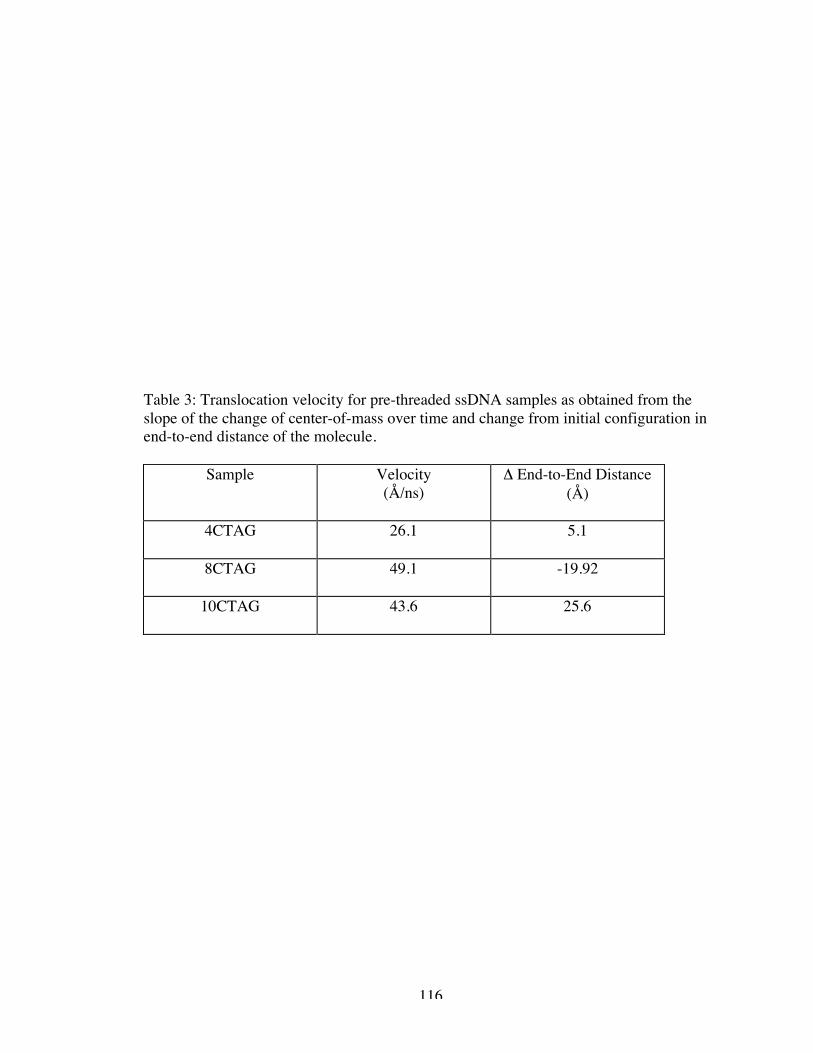
116
Table 3: Translocation velocity for pre-threaded ssDNA samples as obtained from theslope of the change of center-of-mass over time and change from initial configuration inend-to-end distance of the molecule.
Sample Velocity(Å/ns)
Δ End-to-End Distance(Å)
4CTAG 26.1 5.1
8CTAG 49.1 -19.92
10CTAG 43.6 25.6
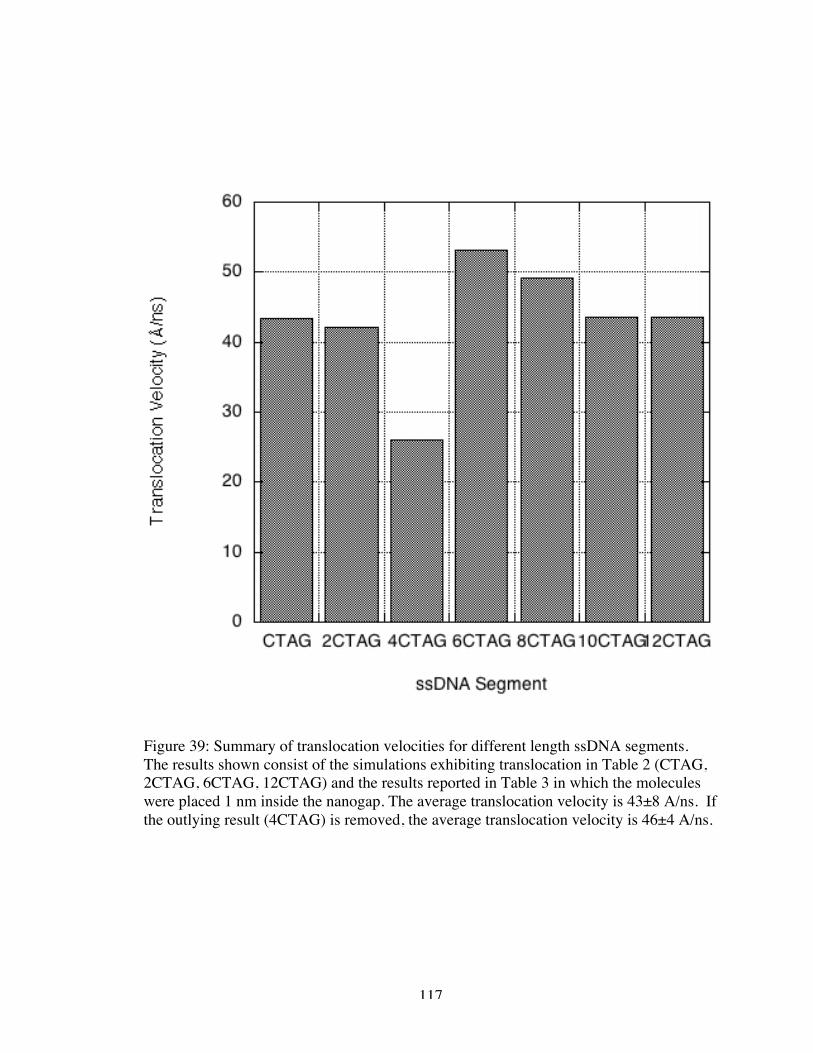
117
Figure 39: Summary of translocation velocities for different length ssDNA segments.The results shown consist of the simulations exhibiting translocation in Table 2 (CTAG,2CTAG, 6CTAG, 12CTAG) and the results reported in Table 3 in which the moleculeswere placed 1 nm inside the nanogap. The average translocation velocity is 43±8 A/ns. Ifthe outlying result (4CTAG) is removed, the average translocation velocity is 46±4 A/ns.
118
CHAPTER VII
CONCLUSIONS
VII.1 Synopsis
We have developed molecular dynamics simulations based on a conceptual device design
for rapid sequencing of DNA. Preliminary simulations led to the search for more
applicable metal/non-metal potentials to describe the interactions with the electrodes. We
also performed electrophoretic simulations of DNA in bulk to compare simulation values
for translocation velocity to experimental values through extrapolation. This ensured that
the velocity values we obtained through simulation were within reasonable bounds.
Following initial investigatory simulations, we began full-scale simulations of the
device concept using the electrode charge dynamics method to accurately describe
metal/non-metal interactions with the intention of developing relationships between
design variables and translocation behavior. Application of applied external electric
fields illustrated that this method of control can be used to force ssDNA to translocate
through a nanoscale gap; however, a clear relationship (i.e. linear or non-linear equation)
was not obtained. There exist several factors including energetic barriers to nanopore
translocation and molecular attraction to metal electrodes that have been prohibitive in
developing this relationship. It was clear from this study, though, that electrode charge
dynamics was the appropriate interaction potential for future simulations of this device.
Further design variable study led to the examination of the electrode gap width
and it effect on allowing translocation of the ssDNA molecule. We found a heuristic
119
value for which the molecule will no longer translocate over the course of our
nanosecond simulations. Widths larger than this value appear to have little effect on
translocation speed. This value, 2.5 nm, happens to be slightly larger than previous
studies of DNA translocation through synthetic nanopores. However, there are many
differences in the simulations to consider including the ssDNA, the initial conditions,
pore geometry and nature of the pore making direct comparisons difficult.
This final variable we considered was the length of the ssDNA sample. Realistic
applications of this device will use DNA strands that are infinitely long on the molecular
dynamics scale. We evaluated the translocation behavior of strands varying from 4 to 48
nucleotides, being limited by the electrostatic cutoff value and physical limitations of the
simulated device as well as computational resources. We were unable to conclusively
evaluate the effect of changing length strand (without pre-threading the sample) on
translocation velocity due to the molecule’s affinity for the electrodes. Pre-threading of
the sample allowed for successful translocation in most cases and the resulting velocities
suggest chain length has little influence on translocation velocity at nanoscale sample
sizes. Attempting to overcome molecular deformation though the implementation of
shaped electrodes, we were similarly unable to avoid the molecular attraction of the
ssDNA to the metal electrodes. This affinity is well know in literature65-69 and must be
overcome through other methods in the future, such as using nanofluidic transport to the
electrode so that the molecule arrives at the electrode in an extended conformation.
120
VII.2 Future Work
There exist several opportunities for continuation and extension of the work presented in
this dissertation. A significant addition would include ensemble averaging of the
individual simulations, though this would require significantly more computational
resources than we currently have available. Ensemble averaging would possibly allow
for the evaluation of a translocation velocity-length relationship in the case of the
variable sample length simulations. Should a velocity-length relationship be developed,
one could then compare the results to a mathematical model for polymer translocation
through a long nanopore73 which predicts two regimes of behavior based on polymer
length and pore size.
The original concept called for the use of both platinum and gold electrodes for
experimental implementation. Obtaining ECD parameters for gold atoms would make
simulations line up even closer with the conceptual vision of the device. These
parameters would also be of use for future simulations in different applications.
Extension of this project could easily be accomplished through evaluation of more
device design variables. The solvent used in all simulations presented here was pure
water. Evaluation of various viscosities (i.e. different solvents) and their effects on
translocation could prove beneficial in determining ideal motive force. Presumably, the
ideal applied electric field will also be dependent on solvent viscosity. Additional
simulations investigating the shape of the electrodes may also be of value.
Finally, we believe it will be necessary to include some form of nanofluidic
focusing device to properly align the strand at the entrance to the nanogap. Simulations
investing the effects of the implementation of fluid flow (using the appropriate interaction

121
potentials) within the device would be of great value. It may even eliminate the need for
an electrical driving force.
122
APPENDIX A
LAMMPS INPUT FILE
I have included here, for reference, a sample input file for use with the modified
version of LAMMPS. This input file was used for the 4CTAG length simulation as
described in Chapter 6. The input first sets about defining basic simulation input values
such as boundary conditions and bond, angle, and dihedral types. Then after reading the
data file, which contains some pair coefficient data, we define more specific interactions
between atoms with the pair_coeff command. Then we use the group command to define
groups of atoms that will be used in applying “fixes”. The chd command is only valid in
the modified LAMMPS version used for this work. It defines the electrode charge
dynamics parameters |e| and γ and the atom type to which ECD is applied. We then apply
our “fixes” which include NVT, SHAKE, and ECD. The run is performed in sections as
presented here because of the extremely large size of the dump files. The ACCRE file
system, and most LINUX machines, does not allow single files to be larger than 2GB in
size without special compilation consideration. The equilibration occurs over 400,000
timesteps of varying sizes before the electric field is applied through a fix. The
remaining dump files are the output of the production run of 1 ns.
units realneigh_modify delay 5 every 1boundary p p f
atom_style hybrid full chdbond_style harmonicangle_style charmmdihedral_style charmmimproper_style harmonic
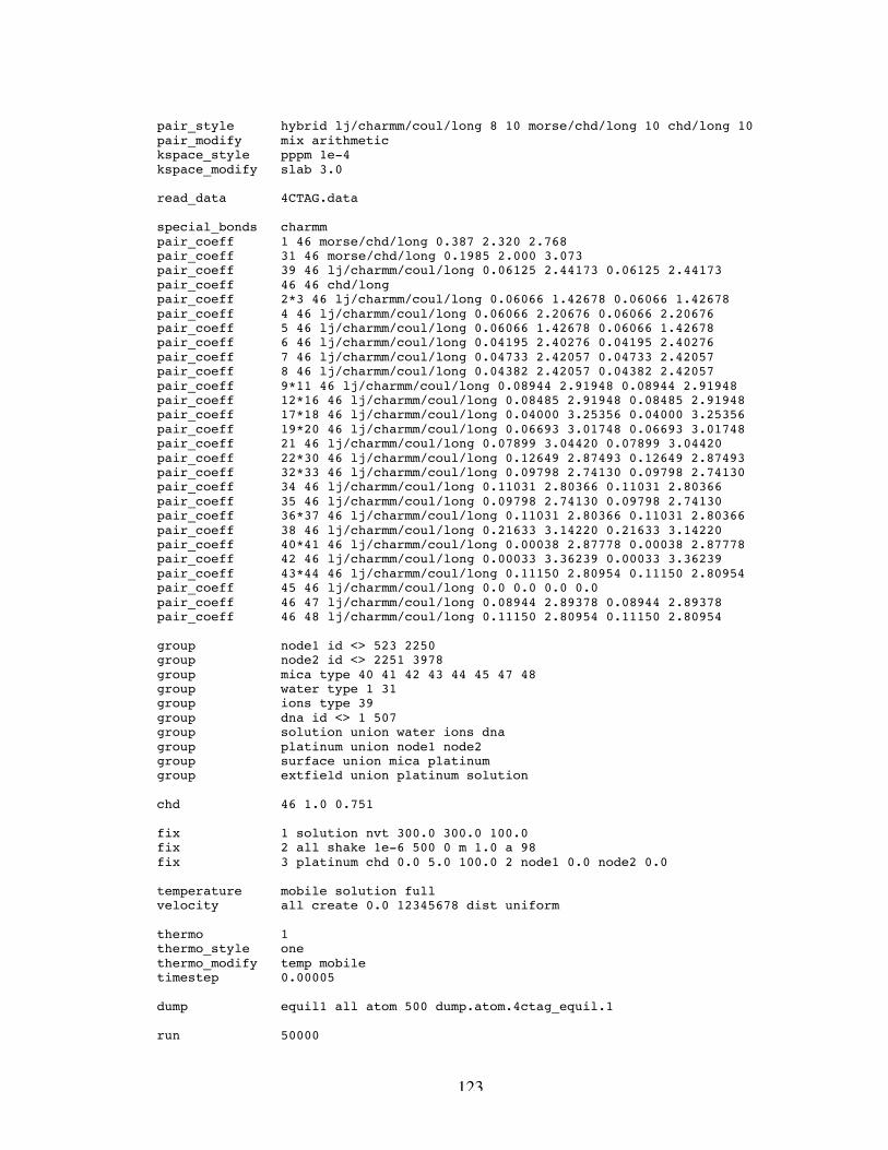
123
pair_style hybrid lj/charmm/coul/long 8 10 morse/chd/long 10 chd/long 10pair_modify mix arithmetickspace_style pppm 1e-4kspace_modify slab 3.0
read_data 4CTAG.data
special_bonds charmmpair_coeff 1 46 morse/chd/long 0.387 2.320 2.768pair_coeff 31 46 morse/chd/long 0.1985 2.000 3.073pair_coeff 39 46 lj/charmm/coul/long 0.06125 2.44173 0.06125 2.44173pair_coeff 46 46 chd/longpair_coeff 2*3 46 lj/charmm/coul/long 0.06066 1.42678 0.06066 1.42678pair_coeff 4 46 lj/charmm/coul/long 0.06066 2.20676 0.06066 2.20676pair_coeff 5 46 lj/charmm/coul/long 0.06066 1.42678 0.06066 1.42678pair_coeff 6 46 lj/charmm/coul/long 0.04195 2.40276 0.04195 2.40276pair_coeff 7 46 lj/charmm/coul/long 0.04733 2.42057 0.04733 2.42057pair_coeff 8 46 lj/charmm/coul/long 0.04382 2.42057 0.04382 2.42057pair_coeff 9*11 46 lj/charmm/coul/long 0.08944 2.91948 0.08944 2.91948pair_coeff 12*16 46 lj/charmm/coul/long 0.08485 2.91948 0.08485 2.91948pair_coeff 17*18 46 lj/charmm/coul/long 0.04000 3.25356 0.04000 3.25356pair_coeff 19*20 46 lj/charmm/coul/long 0.06693 3.01748 0.06693 3.01748pair_coeff 21 46 lj/charmm/coul/long 0.07899 3.04420 0.07899 3.04420pair_coeff 22*30 46 lj/charmm/coul/long 0.12649 2.87493 0.12649 2.87493pair_coeff 32*33 46 lj/charmm/coul/long 0.09798 2.74130 0.09798 2.74130pair_coeff 34 46 lj/charmm/coul/long 0.11031 2.80366 0.11031 2.80366pair_coeff 35 46 lj/charmm/coul/long 0.09798 2.74130 0.09798 2.74130pair_coeff 36*37 46 lj/charmm/coul/long 0.11031 2.80366 0.11031 2.80366pair_coeff 38 46 lj/charmm/coul/long 0.21633 3.14220 0.21633 3.14220pair_coeff 40*41 46 lj/charmm/coul/long 0.00038 2.87778 0.00038 2.87778pair_coeff 42 46 lj/charmm/coul/long 0.00033 3.36239 0.00033 3.36239pair_coeff 43*44 46 lj/charmm/coul/long 0.11150 2.80954 0.11150 2.80954pair_coeff 45 46 lj/charmm/coul/long 0.0 0.0 0.0 0.0pair_coeff 46 47 lj/charmm/coul/long 0.08944 2.89378 0.08944 2.89378pair_coeff 46 48 lj/charmm/coul/long 0.11150 2.80954 0.11150 2.80954
group node1 id <> 523 2250group node2 id <> 2251 3978group mica type 40 41 42 43 44 45 47 48group water type 1 31group ions type 39group dna id <> 1 507group solution union water ions dnagroup platinum union node1 node2group surface union mica platinumgroup extfield union platinum solution
chd 46 1.0 0.751
fix 1 solution nvt 300.0 300.0 100.0fix 2 all shake 1e-6 500 0 m 1.0 a 98fix 3 platinum chd 0.0 5.0 100.0 2 node1 0.0 node2 0.0
temperature mobile solution fullvelocity all create 0.0 12345678 dist uniform
thermo 1thermo_style onethermo_modify temp mobiletimestep 0.00005
dump equil1 all atom 500 dump.atom.4ctag_equil.1
run 50000
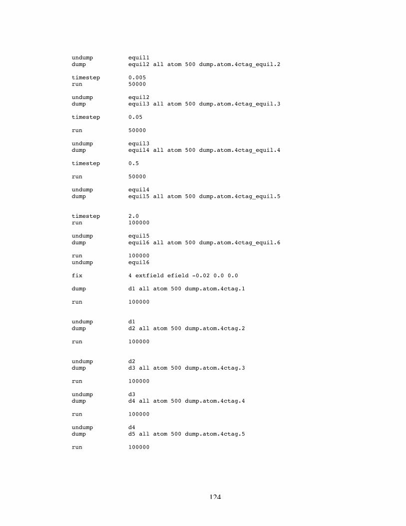
124
undump equil1dump equil2 all atom 500 dump.atom.4ctag_equil.2
timestep 0.005run 50000
undump equil2dump equil3 all atom 500 dump.atom.4ctag_equil.3
timestep 0.05
run 50000
undump equil3dump equil4 all atom 500 dump.atom.4ctag_equil.4
timestep 0.5
run 50000
undump equil4dump equil5 all atom 500 dump.atom.4ctag_equil.5
timestep 2.0run 100000
undump equil5dump equil6 all atom 500 dump.atom.4ctag_equil.6
run 100000undump equil6
fix 4 extfield efield -0.02 0.0 0.0
dump d1 all atom 500 dump.atom.4ctag.1
run 100000
undump d1dump d2 all atom 500 dump.atom.4ctag.2
run 100000
undump d2dump d3 all atom 500 dump.atom.4ctag.3
run 100000
undump d3dump d4 all atom 500 dump.atom.4ctag.4
run 100000
undump d4dump d5 all atom 500 dump.atom.4ctag.5
run 100000
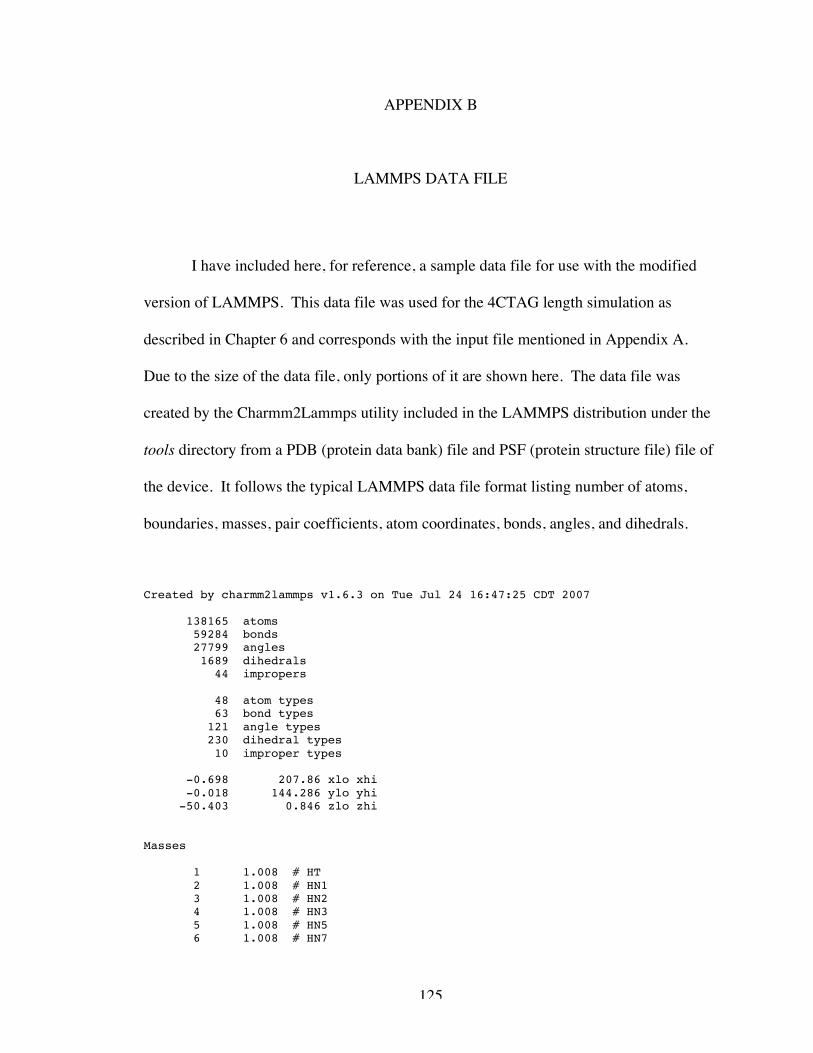
125
APPENDIX B
LAMMPS DATA FILE
I have included here, for reference, a sample data file for use with the modified
version of LAMMPS. This data file was used for the 4CTAG length simulation as
described in Chapter 6 and corresponds with the input file mentioned in Appendix A.
Due to the size of the data file, only portions of it are shown here. The data file was
created by the Charmm2Lammps utility included in the LAMMPS distribution under the
tools directory from a PDB (protein data bank) file and PSF (protein structure file) file of
the device. It follows the typical LAMMPS data file format listing number of atoms,
boundaries, masses, pair coefficients, atom coordinates, bonds, angles, and dihedrals.
Created by charmm2lammps v1.6.3 on Tue Jul 24 16:47:25 CDT 2007
138165 atoms 59284 bonds 27799 angles 1689 dihedrals 44 impropers
48 atom types 63 bond types 121 angle types 230 dihedral types 10 improper types
-0.698 207.86 xlo xhi -0.018 144.286 ylo yhi -50.403 0.846 zlo zhi
Masses
1 1.008 # HT 2 1.008 # HN1 3 1.008 # HN2 4 1.008 # HN3 5 1.008 # HN5 6 1.008 # HN7
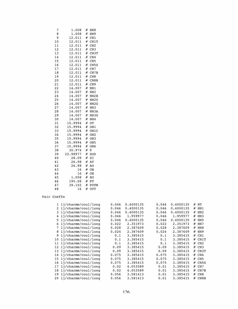
126
7 1.008 # HN8 8 1.008 # HN9 9 12.011 # CN1 10 12.011 # CN1T 11 12.011 # CN2 12 12.011 # CN3 13 12.011 # CN3T 14 12.011 # CN4 15 12.011 # CN5 16 12.011 # CN5G 17 12.011 # CN7 18 12.011 # CN7B 19 12.011 # CN8 20 12.011 # CN8B 21 12.011 # CN9 22 14.007 # NN1 23 14.007 # NN2 24 14.007 # NN2B 25 14.007 # NN2U 26 14.007 # NN2G 27 14.007 # NN3 28 14.007 # NN3A 29 14.007 # NN3G 30 14.007 # NN4 31 15.9994 # OT 32 15.9994 # ON1 33 15.9994 # ON1C 34 15.9994 # ON2 35 15.9994 # ON3 36 15.9994 # ON5 37 15.9994 # ON6 38 30.974 # P 39 22.98977 # SOD 40 28.09 # SI 41 26.98 # AT 42 26.98 # AO 43 16 # OB 44 16 # OH 45 1.008 # HO 46 195.08 # PT 47 39.102 # POTM 48 16 # OTT
Pair Coeffs
1 lj/charmm/coul/long 0.046 0.4000135 0.046 0.4000135 # HT 2 lj/charmm/coul/long 0.046 0.4000135 0.046 0.4000135 # HN1 3 lj/charmm/coul/long 0.046 0.4000135 0.046 0.4000135 # HN2 4 lj/charmm/coul/long 0.046 1.959977 0.046 1.959977 # HN3 5 lj/charmm/coul/long 0.046 0.4000135 0.046 0.4000135 # HN5 6 lj/charmm/coul/long 0.022 2.351973 0.022 2.351973 # HN7 7 lj/charmm/coul/long 0.028 2.387609 0.028 2.387609 # HN8 8 lj/charmm/coul/long 0.024 2.387609 0.024 2.387609 # HN9 9 lj/charmm/coul/long 0.1 3.385415 0.1 3.385415 # CN1 10 lj/charmm/coul/long 0.1 3.385415 0.1 3.385415 # CN1T 11 lj/charmm/coul/long 0.1 3.385415 0.1 3.385415 # CN2 12 lj/charmm/coul/long 0.09 3.385415 0.09 3.385415 # CN3 13 lj/charmm/coul/long 0.09 3.385415 0.09 3.385415 # CN3T 14 lj/charmm/coul/long 0.075 3.385415 0.075 3.385415 # CN4 15 lj/charmm/coul/long 0.075 3.385415 0.075 3.385415 # CN5 16 lj/charmm/coul/long 0.075 3.385415 0.075 3.385415 # CN5G 17 lj/charmm/coul/long 0.02 4.053589 0.01 3.385415 # CN7 18 lj/charmm/coul/long 0.02 4.053589 0.01 3.385415 # CN7B 19 lj/charmm/coul/long 0.056 3.581413 0.01 3.385415 # CN8 20 lj/charmm/coul/long 0.056 3.581413 0.01 3.385415 # CN8B
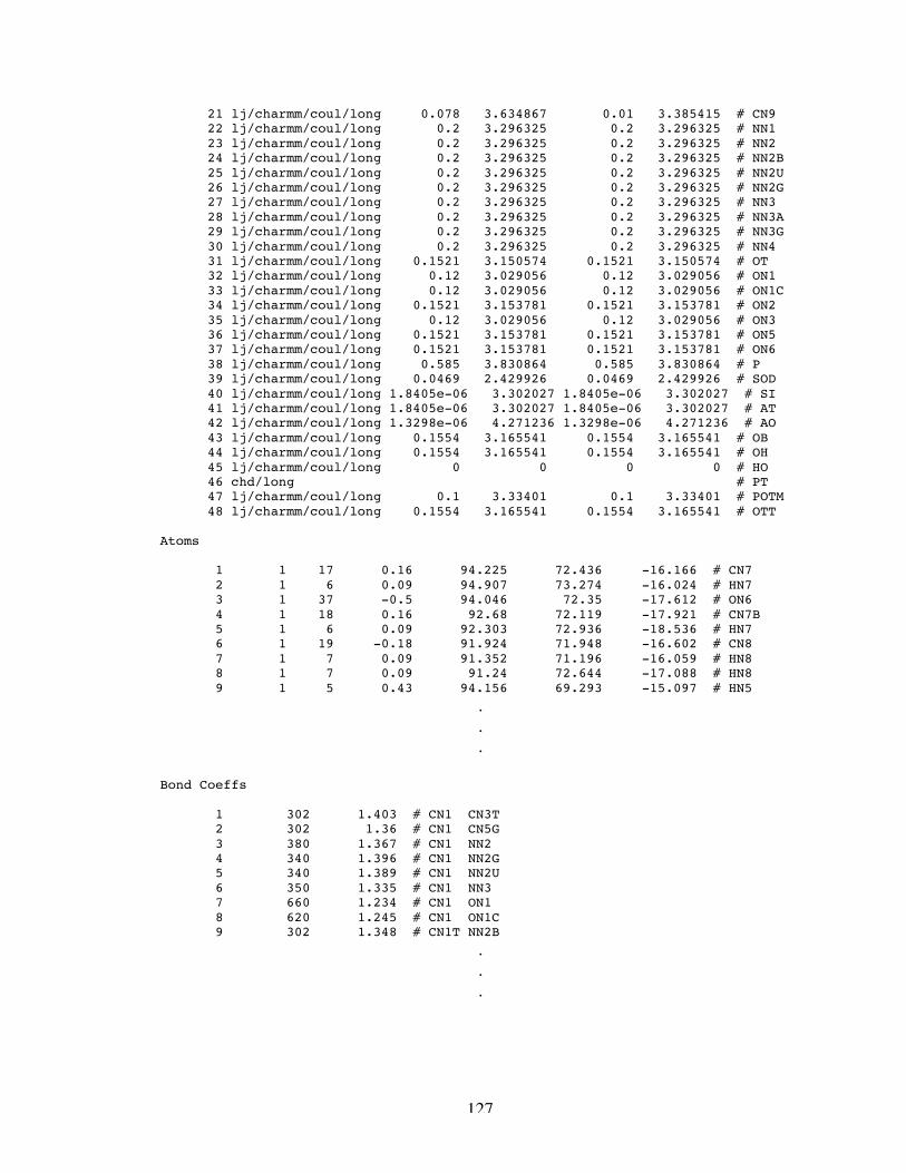
127
21 lj/charmm/coul/long 0.078 3.634867 0.01 3.385415 # CN9 22 lj/charmm/coul/long 0.2 3.296325 0.2 3.296325 # NN1 23 lj/charmm/coul/long 0.2 3.296325 0.2 3.296325 # NN2 24 lj/charmm/coul/long 0.2 3.296325 0.2 3.296325 # NN2B 25 lj/charmm/coul/long 0.2 3.296325 0.2 3.296325 # NN2U 26 lj/charmm/coul/long 0.2 3.296325 0.2 3.296325 # NN2G 27 lj/charmm/coul/long 0.2 3.296325 0.2 3.296325 # NN3 28 lj/charmm/coul/long 0.2 3.296325 0.2 3.296325 # NN3A 29 lj/charmm/coul/long 0.2 3.296325 0.2 3.296325 # NN3G 30 lj/charmm/coul/long 0.2 3.296325 0.2 3.296325 # NN4 31 lj/charmm/coul/long 0.1521 3.150574 0.1521 3.150574 # OT 32 lj/charmm/coul/long 0.12 3.029056 0.12 3.029056 # ON1 33 lj/charmm/coul/long 0.12 3.029056 0.12 3.029056 # ON1C 34 lj/charmm/coul/long 0.1521 3.153781 0.1521 3.153781 # ON2 35 lj/charmm/coul/long 0.12 3.029056 0.12 3.029056 # ON3 36 lj/charmm/coul/long 0.1521 3.153781 0.1521 3.153781 # ON5 37 lj/charmm/coul/long 0.1521 3.153781 0.1521 3.153781 # ON6 38 lj/charmm/coul/long 0.585 3.830864 0.585 3.830864 # P 39 lj/charmm/coul/long 0.0469 2.429926 0.0469 2.429926 # SOD 40 lj/charmm/coul/long 1.8405e-06 3.302027 1.8405e-06 3.302027 # SI 41 lj/charmm/coul/long 1.8405e-06 3.302027 1.8405e-06 3.302027 # AT 42 lj/charmm/coul/long 1.3298e-06 4.271236 1.3298e-06 4.271236 # AO 43 lj/charmm/coul/long 0.1554 3.165541 0.1554 3.165541 # OB 44 lj/charmm/coul/long 0.1554 3.165541 0.1554 3.165541 # OH 45 lj/charmm/coul/long 0 0 0 0 # HO 46 chd/long # PT 47 lj/charmm/coul/long 0.1 3.33401 0.1 3.33401 # POTM 48 lj/charmm/coul/long 0.1554 3.165541 0.1554 3.165541 # OTT
Atoms
1 1 17 0.16 94.225 72.436 -16.166 # CN7 2 1 6 0.09 94.907 73.274 -16.024 # HN7 3 1 37 -0.5 94.046 72.35 -17.612 # ON6 4 1 18 0.16 92.68 72.119 -17.921 # CN7B 5 1 6 0.09 92.303 72.936 -18.536 # HN7 6 1 19 -0.18 91.924 71.948 -16.602 # CN8 7 1 7 0.09 91.352 71.196 -16.059 # HN8 8 1 7 0.09 91.24 72.644 -17.088 # HN8 9 1 5 0.43 94.156 69.293 -15.097 # HN5
.
.
.
Bond Coeffs
1 302 1.403 # CN1 CN3T 2 302 1.36 # CN1 CN5G 3 380 1.367 # CN1 NN2 4 340 1.396 # CN1 NN2G 5 340 1.389 # CN1 NN2U 6 350 1.335 # CN1 NN3 7 660 1.234 # CN1 ON1 8 620 1.245 # CN1 ON1C 9 302 1.348 # CN1T NN2B
.
.
.
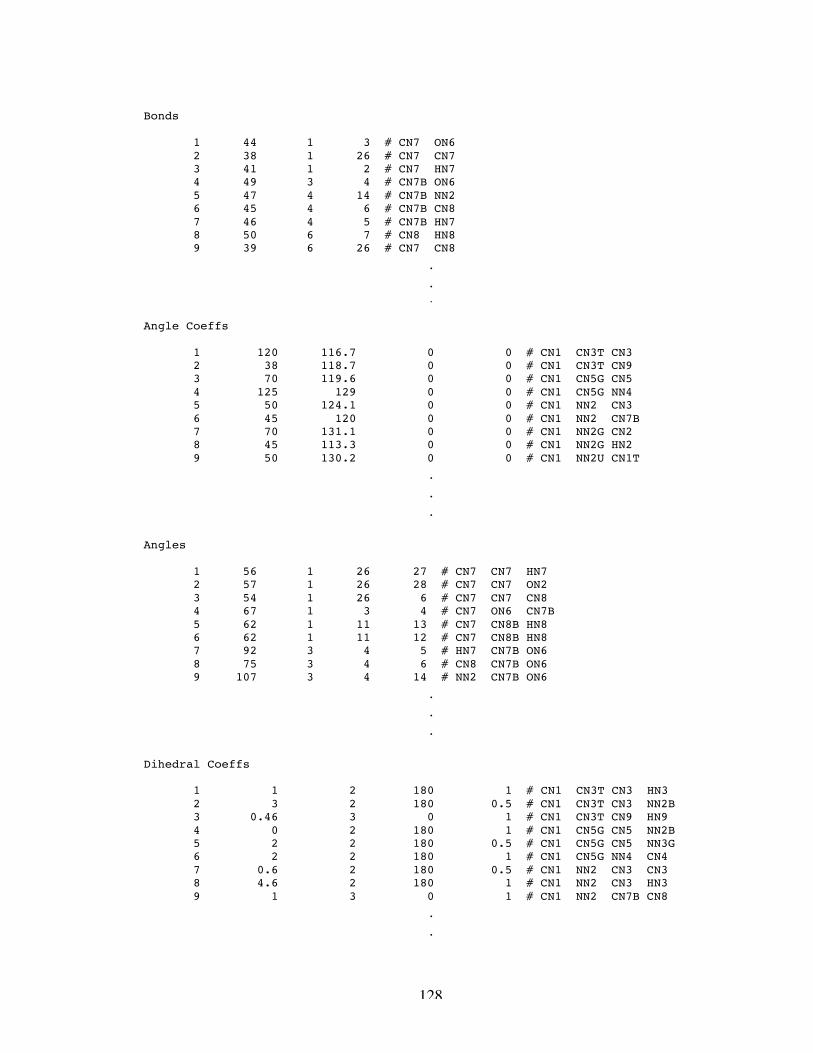
128
Bonds
1 44 1 3 # CN7 ON6 2 38 1 26 # CN7 CN7 3 41 1 2 # CN7 HN7 4 49 3 4 # CN7B ON6 5 47 4 14 # CN7B NN2 6 45 4 6 # CN7B CN8 7 46 4 5 # CN7B HN7 8 50 6 7 # CN8 HN8 9 39 6 26 # CN7 CN8
.
.
.
Angle Coeffs
1 120 116.7 0 0 # CN1 CN3T CN3 2 38 118.7 0 0 # CN1 CN3T CN9 3 70 119.6 0 0 # CN1 CN5G CN5 4 125 129 0 0 # CN1 CN5G NN4 5 50 124.1 0 0 # CN1 NN2 CN3 6 45 120 0 0 # CN1 NN2 CN7B 7 70 131.1 0 0 # CN1 NN2G CN2 8 45 113.3 0 0 # CN1 NN2G HN2 9 50 130.2 0 0 # CN1 NN2U CN1T
.
.
.
Angles
1 56 1 26 27 # CN7 CN7 HN7 2 57 1 26 28 # CN7 CN7 ON2 3 54 1 26 6 # CN7 CN7 CN8 4 67 1 3 4 # CN7 ON6 CN7B 5 62 1 11 13 # CN7 CN8B HN8 6 62 1 11 12 # CN7 CN8B HN8 7 92 3 4 5 # HN7 CN7B ON6 8 75 3 4 6 # CN8 CN7B ON6 9 107 3 4 14 # NN2 CN7B ON6
.
.
.
Dihedral Coeffs
1 1 2 180 1 # CN1 CN3T CN3 HN3 2 3 2 180 0.5 # CN1 CN3T CN3 NN2B 3 0.46 3 0 1 # CN1 CN3T CN9 HN9 4 0 2 180 1 # CN1 CN5G CN5 NN2B 5 2 2 180 0.5 # CN1 CN5G CN5 NN3G 6 2 2 180 1 # CN1 CN5G NN4 CN4 7 0.6 2 180 0.5 # CN1 NN2 CN3 CN3 8 4.6 2 180 1 # CN1 NN2 CN3 HN3 9 1 3 0 1 # CN1 NN2 CN7B CN8
.
.
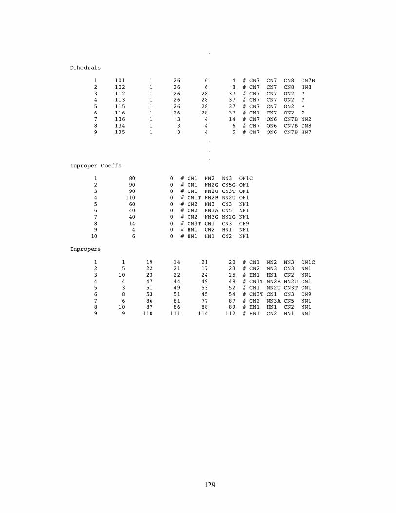
129
.
Dihedrals
1 101 1 26 6 4 # CN7 CN7 CN8 CN7B 2 102 1 26 6 8 # CN7 CN7 CN8 HN8 3 112 1 26 28 37 # CN7 CN7 ON2 P 4 113 1 26 28 37 # CN7 CN7 ON2 P 5 115 1 26 28 37 # CN7 CN7 ON2 P 6 116 1 26 28 37 # CN7 CN7 ON2 P 7 136 1 3 4 14 # CN7 ON6 CN7B NN2 8 134 1 3 4 6 # CN7 ON6 CN7B CN8 9 135 1 3 4 5 # CN7 ON6 CN7B HN7
.
.
.Improper Coeffs
1 80 0 # CN1 NN2 NN3 ON1C 2 90 0 # CN1 NN2G CN5G ON1 3 90 0 # CN1 NN2U CN3T ON1 4 110 0 # CN1T NN2B NN2U ON1 5 60 0 # CN2 NN3 CN3 NN1 6 40 0 # CN2 NN3A CN5 NN1 7 40 0 # CN2 NN3G NN2G NN1 8 14 0 # CN3T CN1 CN3 CN9 9 4 0 # HN1 CN2 HN1 NN1 10 6 0 # HN1 HN1 CN2 NN1
Impropers
1 1 19 14 21 20 # CN1 NN2 NN3 ON1C 2 5 22 21 17 23 # CN2 NN3 CN3 NN1 3 10 23 22 24 25 # HN1 HN1 CN2 NN1 4 4 47 44 49 48 # CN1T NN2B NN2U ON1 5 3 51 49 53 52 # CN1 NN2U CN3T ON1 6 8 53 51 45 54 # CN3T CN1 CN3 CN9 7 6 86 81 77 87 # CN2 NN3A CN5 NN1 8 10 87 86 88 89 # HN1 HN1 CN2 NN1 9 9 110 111 114 112 # HN1 CN2 HN1 NN1
130
APPENDIX C
NONLINEAR ELECTRIC FIELD EFFECTS
Here, we will present a brief description of the molecular basis for the nonlinear
field effects such as those observed in the large magnitude applied electric field
simulations presented in Chapter IV.
It is well known that thermodynamic systems’ fluctuations in flux can be
described by a linearly proportional relationship of the transport coefficient with the
corresponding applied field74. This relationship holds true in the limiting case of a
sufficiently small applied field. The standard chemical engineering example of this
relationship is Newton’s law of viscosity, where shear stress, τξψ, is linearly proportional
to the strain rate, dux dy = &γ , through the relationship
τ xy = −η &γ (20)
where η is the shear viscosity. In the linear (i.e., Newtonian) regime, η does not depend
on &γ , and τ xy is linear in &γ . However, as the strain rate increases, we know to expect
the shear stress to exhibit nonlinear strain-rate dependence, resulting in a strain-rate-
dependent viscosity. This is the non-linear regime, and in this regime the fluid is
described as being non-Newtonian. Generally, the onset of non-linear shear response
occurs then the strain rate exceeds τ −1 , where τ is the longest relaxation time in the
system. Hence at the molecular scale it corresponds to shear rates so large that the
molecules cannot relax into their equilibrium shapes when moving between different
131
locations in the strain field. These effects are most striking in polymers, where the
relaxation times can be very long (and hence the strain rate needed to induce non-linear
behavior is not very large) and where the conformational molecular changes in large
strain fields (the polymer molecules stretch out to align with the strain field) give rise to
large non-linear effects in the viscosity.
The same can be said for any equilibrium system under the influence of and
applied external field, whether it be mechanical or thermal, including the relationship of
drift velocity to electrophoretic mobility and applied electric field as described in
Equation 6. As the applied field increases to the nonlinear regime, the proportionality
constant, electrophoretic mobility in this case, becomes a function of the applied field and
no longer results in linear flux behavior. This is behavior is apparent in the molecular
conformation through alignment and elongation of the molecule with increasing external
applied field. We should also see some alignment of the water molecules in response to
the increasing external field75, though we have not made a point of studying this
molecular configuration. This behavior has been previously documented in many
different systems76-80 and is described in significant detail by Evans and Morriss81.
132
REFERENCES
1. Venter, J. C.; Adams, M. D.; Myers, E. W.; al., e., The Sequence of the HumanGenome. Science 2001, 291, (5507), 1304-1351.
2. Allen, M. P.; Tildesley, D. J., Computer Simulations of Liquids. Clarendon Press:Oxford, 1987.
3. Zhang, L.; George, B.; Thundat, T.; Lee, J., Measurements of Electrical TransportProperties of Single-Stranded DNA Molecules. Submitted for publication.
4. Meller, A.; Nivon, L.; Branton, D., Voltage-Driven DNA Translocations Througha Nanopore. Physical Review Letters 2001, 86, (15), 3435-3438.
5. Heng, J. B.; Ho, C.; Kim, T.; Timp, R.; Aksimentiev, A.; Grinkova, Y. V.; Sligar,S.; Schulten, K.; Timp, G., Sizing DNA Using a Nanometer-Diameter Pore. Biophys. J.2004, 87, (4), 2905-2911.
6. Storm, A.; Chen, J.; Zandbergen, H.; Dekker, C., Translocation of Double-StrandDNA Through a Silicon Oxide Nanopore. Physical Review E 2005, 71, 051903.
7. Storm, A. J.; Storm, C.; Chen, J.; Zandbergen, H.; Joanny, J. F.; Dekker, C., FastDNA Translocation through a Solid-State Nanopore. Nano Lett. 2005, 5, (7), 1193-1197.
8. Fan, R.; Karnik, R.; Yue, M.; Li, D.; Majumdar, A.; Yang, P., DNA Translocationin Inorganic Nanotubes. Nano Lett. 2005, 5, (9), 1633-1637.
9. Fologea, D.; Gershow, M.; Ledden, B.; McNabb, D. S.; Golovchenko, J. A.; Li,J., Detecting Single Stranded DNA with a Solid State Nanopore. Nano Lett. 2005, 5, (10),1905-1909.
10. Sung, W.; Park, P. J., Polymer Translocation through a Pore in a Membrane.Physical Review Letters 1996, 77, (4), 783.
11. Lubensky, D. K.; Nelson, D. R., Driven Polymer Translocation Through a NarrowPore. Biophys. J. 1999, 77, (4), 1824-1838.
133
12. Kong, C. Y.; Muthukumar, M., Modeling of polynucleotide translocation throughprotein pores and nanotubes. ELECTROPHORESIS 2002, 23, (16), 2697-2703.
13. Butler, T. Z.; Gundlach, J. H.; Troll, M. A., Determination of RNA Orientationduring Translocation through a Biological Nanopore. Biophys. J. 2006, 90, (1), 190-199.
14. Yeh, I.-C.; Hummer, G., Diffusion and Electrophoretic Mobility of Single-Stranded RNA from Molecular Dynamics Simulations. Biophys. J. 2004, 86, (2), 681-689.
15. Lee, J. W.; Greenbaum, E., 1999. Programmable Nanometer-Scale Metal Bondingto Single Molecules by Electrolytic Deposition and Depletion. ORNL InventionDisclosure ID 0772;
16. Lee, J. W.; Greenbaum, E. 2002. Programmable Nanometer-Scale ElectrolyticMetal Deposition and Depletion. Office, U. P. 6,447,663 B1.
17. Lagerqvist, J.; Zwolak, M.; DiVentra, M., Fast DNA Sequencing via TransverseElectronic Transport. Nano Lett. 2006, 6, (4), 779-782.
18. Lagerqvist, J.; Zwolak, M.; Di Ventra, M., Influence of the Environment andProbes on Rapid DNA Sequencing via Transverse Electronic Transport. Biophys. J. 2007,93, (7), 2384-2390.
19. Zhang, X. G.; Krstic, P. S.; Zikic, R.; Wells, J. C.; Fuentes-Cabrera, M., First-Principles Transversal DNA Conductance Deconstructed. Biophys. J. 2006, 91, (1), L04-6.
20. Lee, J.; Thundat, T.; Greenbaum, E., 2001. DNA and RNA Sequencing byNanoscale Reading Through Programmable Electrophoresis and Nanoelectrode-GatedTunneling and Dielectric Detection. ORNL Invention Disclosure ID 0943; US PatentAppl. Publ. (2003), 24 pp. CODEN: USXXCO US 2003141189 A1.
21. Leng, Y.; Cummings, P. T., Fluidity of Hydration Layers Nanoconfined betweenMica Surfaces. Physical Review Letters 2005, 94, (2), 026101-4.
22. Franklin, R.; Gosling, R., Molecular Configuration in Sodium Thymonucleate.Nature 1953, 171, 740.
134
23. Swope, W. C.; Andersen, H. C.; Berens, P. H.; Wilson, K. R., A computersimulations method for the calculations of equilibrium constants for the formations ofphysical clusters of molecules: Application to small water clusters. J. Chem. Phys. 1982,76, 637-649.
24. Plimpton, S., Fast Parallel Algorithms for Short-Range Molecular Dynamics.Journal of Computational Physics 1995, 117, (1), 1-19.
25. Plimpton, S.; LAMMPS. http://lammps.sandia.gov
26. Foloppe, N.; MacKerell, A. D., All-atom empirical force field for nucleic acids: I.Parameter optimization based on small molecule and condensed phase macromoleculartarget data. Journal of Computational Chemistry 2000, 21, (2), 86-104.
27. MacKerell, A. D.; Banavali, N. K., All-atom empirical force field for nucleicacids: II. Application to molecular dynamics simulations of DNA and RNA in solution.Journal of Computational Chemistry 2000, 21, (2), 105-120.
28. Beglov, D.; Roux, B., Finite representation of an infinite bulk system: Solventboundary potential for computer simulations. The Journal of Chemical Physics 1994,100, (12), 9050-9063.
29. Jorgensen, W. L.; Chandrasekhar, J.; Madura, J. D.; Impey, R. W.; Klein, M. L.,Comparison of simple potential functions for simulating liquid water. The Journal ofChemical Physics 1983, 79, (2), 926-935.
30. Cygan, R. T.; Liang, J. J.; Kalinichev, A. G., Molecular Models of Hydroxide,Oxyhydroxide, and Clay Phases and the Development of a General Force Field. J. Phys.Chem. B 2004, 108, (4), 1255-1266.
31. Rappé, A.; Casewit, C.; Colwell, K.; Goddard, W.; Skiff, W., UFF, a FullPeriodic Table Force Field for Molecular Mechanics and Molecular DynamicsSimulations. Journal of the American Chemical Society 1992, 114, 10024-10035.
32. Hockney, R. W.; Eastwood, J. W., Computer Simulation Using Particles.McGraw-Hill International Book co.: New York, 1989.
33. Yeh, I.-C.; Berkowitz, M. L., Ewald summation for systems with slab geometry.The Journal of Chemical Physics 1999, 111, (7), 3155-3162.
135
34. Nosé, S., A molecular dynamics method for simulations in the canonicalensemble. Molecular Physics 1984, 52, 255.
35. Nosé, S., A unified formulation of hte constant temperature molecular dynamicsmethods. The Journal of Chemical Physics 1984, 81, (1), 511-519.
36. Hoover, W. G., Canonical dynamics: Equilibrium phase-space distributions.Physical Review A 1985, 31, (3), 1695.
37. Payne, C. M.; Zhao, X.; Vlcek, L.; Cummings, P. T., Molecular DynamicsSimulation of DNA Translocation through a Copper Nanoelectrode Gap submitted toJournal of Physical Chemistry C.
38. Kasianowicz, J. J.; Brandin, E.; Branton, D.; Deamer, D. W., Characterization ofindividual polynucleotide molecules using a membrane†channel. PNAS 1996, 93, (24),13770-13773.
39. Stellwagen, E.; Stellwagen, N. C., Determining the electrophoretic mobility andtranslational diffusion coefficients of DNA molecules in free solution. Electrophoresis2002, 23, (16), 2794-2803.
40. Jackson, J. D., Classical Electrodynamics. Wiley: New York, 1962.
41. Spohr, E.; Heinzinger, K., Molecular dynamics simulation of a water/metalinterface. Chemical Physics Letters 1986, 123, (3), 218-221.
42. Guymon, C.; Rowley, R.; Harb, J.; Wheeler, D., Simulating an ElectrochemicalInterface Using Charge Dynamics. Condensed Matter Physics 2005, 8, (2), 335-356.
43. Hoagland, D. A.; Arvanitidou, E.; Welch, C., Capillary ElectrophoresisMeasurements of the Free Solution Mobility for Several Model Polyelectrolyte Systems.Macromolecules 1999, 32, 6180-6190.
44. Macke, T.; Case, D. A. In Modeling unusual nucleic acid structures, AmericanChemical Society, Washington, DC, 1998; Leontes, N. B.; J. SantaLucia, J., Eds.Washington, DC, 1998; pp 379-393.
136
45. Macke, T.; Svrcek-Seiler, W. A.; Brown, R. A.; Case, D. A.; The NAB MolecularManipulation Language. http://www.scripps.edu/mb/case/
46. Berendsen, H. J. C.; Postma, J. P. M.; Gunsteren, W. F. v.; DiNola, A.; Haak, J.R., Molecular dynamics with coupling to an external bath. The Journal of ChemicalPhysics 1984, 81, (8), 3684-3690.
47. Martyna, G. J.; Tobias, D. J.; Klein, M. L., Constant pressure molecular dynamicsalgorithms. The Journal of Chemical Physics 1994, 101, (5), 4177-4189.
48. Ryckaert, J.-P.; Ciccotti, G.; Berendsen, H. J. C., Numerical integration of thecartesian equations of motion of a system with constraints: molecular dynamics of n-alkanes. Journal of Computational Physics 1977, 23, (3), 327-341.
49. Dukhin, A. S.; Dukhin, S. S., Aperiodic capillary electrophoresis method using analternating current electric field for separation of macromolecules. Electrophoresis 2005,26, (11), 2149-2153.
50. Raviv, U.; Klein, J., Fluidity of Bound Hydration Layers. Science 2002, 297,(5586), 1540-1543.
51. Leng, Y.; Cummings, P. T., Fluidity of Hydration Layers Nanoconfined betweenMica Surfaces. Physical Review Letters 2005, 94, (2), 026101.
52. Leng, Y.; Cummings, P. T., Hydration structure of water confined between micasurfaces. The Journal of Chemical Physics 2006, 124, (7), 074711.
53. Rappe, A. K.; Colwell, K. S.; Casewit, C. J., Application of a universal force fieldto metal complexes. Inorg. Chem. 1993, 32, (16), 3438-3450.
54. Boyd, P. D. W.; Hodgson, M. C.; Rickard, C. E. F.; Oliver, A. G.; Chaker, L.;Brothers, P. J.; Bolskar, R. D.; Tham, F. S.; Reed, C. A., Selective SupramolecularPorphyrin/Fullerene Interactions. J. Am. Chem. Soc. 1999, 121, (45), 10487-10495.
55. Fa, W.; Chen, J.; Liu, H.; Dong, J., Structural and electronic properties of themetal-metal intramoleular junctions of single-walled carbon nanotubes. Physical ReviewB (Condensed Matter and Materials Physics) 2004, 69, (23), 235413.
137
56. Felix, V.; Matthews, S. E.; Beer, P. D.; Drew, M. G. B., Selectivity ofcalix[4]tubes towards metal ions: A molecular dynamics study. Physical ChemistryChemical Physics 2002, 4, (15), 3849-3858.
57. Horinek, D.; Michl, J., Surface-mounted altitudinal molecular rotors in alternatingelectric field: Single-molecule parametric oscillator molecular dynamics. Proceedings ofthe National Academy of Sciences 2005, 102, (40), 14175-14180.
58. Evans, D. J.; Searles, D. J., Equilibrium microstates which generate second lawviolating steady states. Physical Review E 1994, 50, (2), 1645.
59. Evans, D. J.; Searles, D. J., The Fluctuation Theorem. Advances in Physics 2002,51, (7), 1529-1585.
60. Payne, C. M.; Zhao, X.; Cummings, P. T., Molecular simulations of DNAtransport in solution. Molecular Simulation 2007, 33, (4), 399 - 403.
61. Wheeler, D.; Newman, J., Molecular Dynamics Simulations of MulticomponentDiffusion. 2. Nonequilibrium Method. Journal of Physical Chemistry B 2004, 108,18362-18367.
62. Meng, S.; Wang, E. G.; Gao, S., Water adsorption on metal surfaces: A generalpicture from density functional theory studies. Physical Review B 2004, 69, 195404.
63. Heng, J. B.; Aksimentiev, A.; Ho, C.; Marks, P.; Grinkova, Y. V.; Sligar, S.;Schulten, K.; Timp, G., The Electromechanics of DNA in a Synthetic Nanopore. Biophys.J. 2006, 90, (3), 1098-1106.
64. Henrickson, S. E.; Misakian, M.; Robertson, B.; Kasianowicz, J. J., Driven DNATransport into an Asymmetric Nanometer-Scale Pore. Physical Review Letters 2000, 85,(14), 3057.
65. Tsang, S. C.; Guo, Z.; Chen, Y. K.; Green, M. L. H.; Hill, H. A. O.; Hambley, T.W.; Sadler, P. J., Immobilization of Platinated and Iodinated Oligonucleotides on CarbonNanotubes. Angewandte Chemie International Edition in English 1997, 36, (20), 2198-2200.
66. Buzaneva, E.; Karlash, A.; Yakovkin, K.; Shtogun, Y.; Putselyk, S.; Zherebetskiy,D.; Gorchinskiy, A.; Popova, G.; Prilutska, S.; Matyshevska, O.; Prilutskyy, Y.; Lytvyn,
138
P.; Scharff, P.; Eklund, P., DNA nanotechnology of carbon nanotube cells: physico-chemical models of self-organization and properties. Materials Science and Engineering:C 2002, 19, (1-2), 41-45.
67. Zheng, M.; Jagota, A.; Semke, E. D.; Diner, B. A.; McLean, R. S.; Lustig, S. R.;Richardson, R. E.; Tassi, N. G., DNA-assisted dispersion and separation of carbonnanotubes. Nat Mater 2003, 2, (5), 338-342.
68. Gearheart, L. A.; Ploehn, H. J.; Murphy, C. J., Oligonucleotide Adsorption toGold Nanoparticles: A Surface-Enhanced Raman Spectroscopy Study of IntrinsicallyBent DNA. J. Phys. Chem. B 2001, 105, (50), 12609-12615.
69. Mbindyo, J. K. N.; Reiss, B. D.; Martin, B. R.; Keating, C. D.; Natan, M. J.;Mallouk, T. E., DNA-Directed Assembly of Gold Nanowires on ComplementarySurfaces. Advanced Materials 2001, 13, (4), 249-254.
70. Fang, L.; Hu, H.; Larson, R. G., DNA configurations and concentration inshearing flow near a glass surface in a microchannel. Journal of Rheology 2005, 49, (1),127-138.
71. Dukkipati, V. r.; Kim, J. H.; Pang, S. W.; Larson, R. G., Protein-AssistedStretching and Immobilization of DNA Molecules in a Microchannel. Nano Lett. 2006, 6,(11), 2499-2504.
72. Watari, N.; Makino, M.; Kikuchi, N.; Larson, R.; Doi, M., Simulation of DNAmotion in a microchannel using stochastic rotation dynamics. Journal of ChemicalPhysics 2007, 126, 094902.
73. Slonkina, E.; Kolomeisky, A. B., Polymer Translocation Through a LongNanopore. Journal of Chemical Physics 2003, 118, (15), 7112-7118.
74. Kubo, R.; Yokota, M.; Nakajima, S., Statistical-mechanical theory of irreversibleprocesses. II. Response to thermal disturbance. Journal of the Physical Society of Japan1957, 12, (11), 1203-1211.
75. Jung, D. H.; Yang, J. H.; Jhon, M. S., The effect of an external electric field onthe structure of liquid water using molecular dynamics simulations. Chemical Physics1999, 244, 331-337.
139
76. Moore, J. D.; Cui, S. T.; Cochran, H. D.; Cummings, P. T., Rheology of lubricantbasestocks: A molecular dynamics study of C30 isomers. Journal of Chemical Physics2000, 113, (19), 8833-8840.
77. Meyer, B.; Vanderbilt, D., Ab initio study of BaTiO_{3} and PbTiO_{3} surfacesin external electric fields. Physical Review B 2001, 63, (20), 205426.
78. Kawasaki, K.; Gunton, J. D., Theory of Nonlinear Transport Processes: NonlinearShear Viscosity and Normal Stress Effects. Physical Review A 1973, 8, (4), 2048.
79. Gravina, D.; Ciccotti, G.; Holian, B. L., Linear and nonlinear viscous flow in two-dimensional fluids. Physical Review E 1995, 52, (6), 6123.
80. Maginn, E. J.; Bell, A. T.; Theodorou, D. N., Transport diffusivity of methane insilicalite from equilibrium and nonequilibrium simulations. J. Phys. Chem. 1993, 97,(16), 4173-4181.
81. Evans, D. J.; Morriss, G. P., Statistical Mechanics of Nonequilibrium Liquids.Academic Press Inc.: San Diego, 1990.