MOLECULAR DYNAMICS AND CONTINUUM

SIMULATIONS OF FLUID FLOWS WITH SLIP

BOUNDARY CONDITIONS

By

Anoosheh Niavaranikheiri

A DISSERTATION

Submitted to

Michigan State University

in partial fulfillment of the requirements

for the degree of

DOCTOR OF PHILOSOPHY

Mechanical Engineering

2011

ABSTRACT

MOLECULAR DYNAMICS AND CONTINUUM

SIMULATIONS OF FLUID FLOWS WITH SLIP

BOUNDARY CONDITIONS

By

Anoosheh Niavaranikheiri

Microfluidics is a rapidly developing field with applications ranging from molecular biol-

ogy, environmental monitoring, and clinical diagnostics. Microfluidic systems are character-

ized by large surface-to-volume ratios, and, therefore, fluid flows are significantly influenced

by boundary conditions. The fundamental assumption in fluid mechanics is the no-slip

boundary condition, which states that the tangential fluid velocity is equal to the adjacent

wall speed. Although this assumption is successful in describing fluid flows on macroscopic

length scales, recent experimental and numerical studies have shown that it breaks down at

microscopic scales due to the possibility of slip of the fluid relative to the wall. The effect of

slip is more pronounced for highly viscous liquids like polymer melts or in the region near

the moving contact line due to the large gradient in shear stress at the liquid/solid interface.

The measure of slip is the so-called slip length, which is defined as a distance between the

real interface and imaginary plane where the extrapolated velocity profile vanishes. The slip

length value is sensitive to several key parameters, such as surface energy, surface roughness,

fluid structure, and shear rate.

In this dissertation, the slip phenomena in thin liquid films confined by either flat or struc-

tured surfaces are investigated by molecular dynamics (MD) and continuum simulations. It

is found that for flows of both monatomic and polymeric fluids over smooth surfaces, the

slip length depends nonlinearly on shear rate at sufficiently high rates. The laminar flow

away from a curved boundary is usually described by means of the effective slip length,

which is defined with respect to the mean roughness height. MD simulations show that for

corrugated surfaces with wavelength larger than the size of polymer chains, the effective

slip length decreases monotonically with increasing corrugation amplitude. A detailed com-

parison between the solution of the Navier-Stokes equation with the local rate-dependent

slip condition and results of MD simulations indicates that there is excellent agreement

between the velocity profiles and the effective slip lengths at low shear rate and small-scale

surface roughness. It was found that the main cause of the slight discrepancy between MD

and continuum results at high shear rates is the reduction of the local slip length in the

higher pressure regions where the boundary slope becomes relatively large with respect to

the mainstream flow. It was further shown that for the Stokes flow with the local no-slip

boundary condition, the effective slip length decreases with increasing corrugation ampli-

tude and a flow circulation is developed in sufficiently deep grooves. Analysis of a numerical

solution of the Navier-Stokes equation with the local slip condition shows that the inertial

effects promote the asymmetric vortex flow formation and reduce the effective slip length.

TABLE OF CONTENTS

LIST OF TABLES vi

LIST OF FIGURES vii

1 Introduction 1

2 Rheological study of polymer flow past rough surfaces with slip boundary

conditions 4

2.1 Introduction . . . . . . . . . . . . . . . . . . . . . . . . . . . . . . . . . . . . 4

2.2 The details of the numerical simulations . . . . . . . . . . . . . . . . . . . . 7

2.2.1 Molecular dynamics model . . . . . . . . . . . . . . . . . . . . . . . . 7

2.2.2 Continuum method . . . . . . . . . . . . . . . . . . . . . . . . . . . . 8

2.3 MD results for flat walls . . . . . . . . . . . . . . . . . . . . . . . . . . . . . 10

2.4 Results for periodically corrugated walls: large wavelength . . . . . . . . . . 11

2.4.1 MD simulations . . . . . . . . . . . . . . . . . . . . . . . . . . . . . . 11

2.4.2 Comparison between MD and continuum simulations . . . . . . . . . 12

2.5 Results for periodically corrugated walls: small wavelengths . . . . . . . . . 14

2.5.1 Comparison between MD and continuum simulations . . . . . . . . . 14

2.5.2 The polymer chain configuration and dynamics near rough surfaces . 15

2.6 Conclusions . . . . . . . . . . . . . . . . . . . . . . . . . . . . . . . . . . . . 17

3 Slip boundary conditions for shear flow of polymer melts past atomically

flat surfaces 31

3.1 Introduction . . . . . . . . . . . . . . . . . . . . . . . . . . . . . . . . . . . . 31

3.2 Details of molecular dynamics simulations . . . . . . . . . . . . . . . . . . . 33

3.3 Results . . . . . . . . . . . . . . . . . . . . . . . . . . . . . . . . . . . . . . . 36

3.3.1 Fluid density and velocity profiles . . . . . . . . . . . . . . . . . . . . 36

3.3.2 Rate dependence of the slip length and shear viscosity . . . . . . . . 36

3.3.3 Analysis of the fluid structure in the first layer . . . . . . . . . . . . . 39

3.4 Conclusions . . . . . . . . . . . . . . . . . . . . . . . . . . . . . . . . . . . . 41

4 The effective slip length and vortex formation in laminar flow over a rough

surface 54

4.1 Introduction . . . . . . . . . . . . . . . . . . . . . . . . . . . . . . . . . . . . 54

4.2 Details of numerical simulations . . . . . . . . . . . . . . . . . . . . . . . . . 57

4.3 Results . . . . . . . . . . . . . . . . . . . . . . . . . . . . . . . . . . . . . . . 60

4.3.1 Analytical solution of the Stokes equation for viscous flow over a wavy

wall . . . . . . . . . . . . . . . . . . . . . . . . . . . . . . . . . . . . 60

iv

4.3.2 Flow over a rough surface with the local no-slip boundary condition . 60

4.3.3 Effect of the local slip on the flow pattern near the rough surface . . 63

4.3.4 Effect of the Reynolds number on the effective slip length . . . . . . . 65

4.4 Conclusions . . . . . . . . . . . . . . . . . . . . . . . . . . . . . . . . . . . . 67

5 Modeling the combined effect of surface roughness and shear rate on slip

flow of simple fluids 86

5.1 Introduction . . . . . . . . . . . . . . . . . . . . . . . . . . . . . . . . . . . . 86

5.2 The details of numerical methods . . . . . . . . . . . . . . . . . . . . . . . . 89

5.2.1 Molecular dynamics simulations . . . . . . . . . . . . . . . . . . . . . 89

5.2.2 Continuum simulations . . . . . . . . . . . . . . . . . . . . . . . . . . 91

5.3 Results . . . . . . . . . . . . . . . . . . . . . . . . . . . . . . . . . . . . . . . 93

5.3.1 MD simulations: the intrinsic and effective slip lengths . . . . . . . . 93

5.3.2 Comparison between MD and continuum simulations . . . . . . . . . 95

5.3.3 A detailed analysis of the flow near the curved boundary . . . . . . . 96

5.4 Conclusions . . . . . . . . . . . . . . . . . . . . . . . . . . . . . . . . . . . . 100

6 Slip boundary conditions for the moving contact line in molecular dynam-

ics and continuum simulations 116

6.1 Introduction . . . . . . . . . . . . . . . . . . . . . . . . . . . . . . . . . . . . 116

6.2 Molecular dynamics (MD) simulations . . . . . . . . . . . . . . . . . . . . . 118

6.2.1 Equilibrium case . . . . . . . . . . . . . . . . . . . . . . . . . . . . . 118

6.2.2 Shear flow . . . . . . . . . . . . . . . . . . . . . . . . . . . . . . . . . 121

6.3 Details of continuum simulations . . . . . . . . . . . . . . . . . . . . . . . . 123

6.3.1 Fixed grid method for immersed objects . . . . . . . . . . . . . . . . 123

6.3.2 Continuum Results . . . . . . . . . . . . . . . . . . . . . . . . . . . . 127

6.4 Conclusions . . . . . . . . . . . . . . . . . . . . . . . . . . . . . . . . . . . . 128

BIBLIOGRAPHY 145

v

LIST OF TABLES

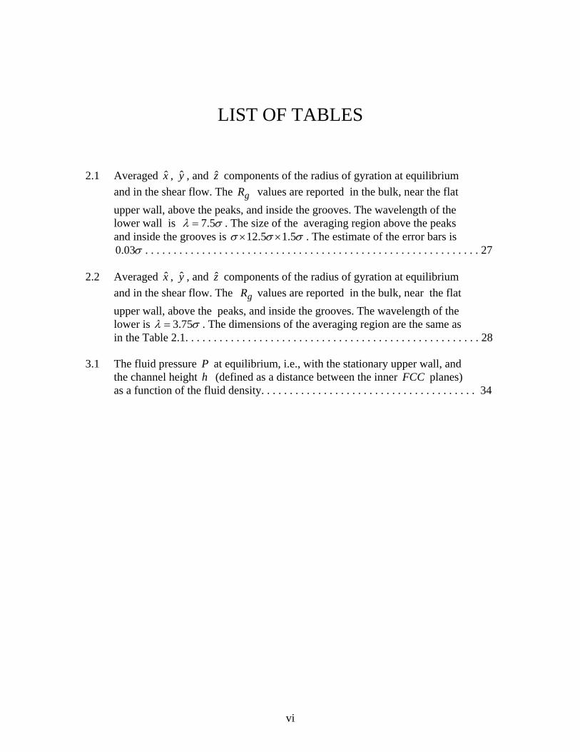
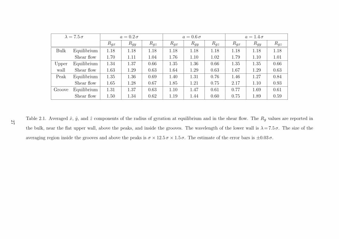
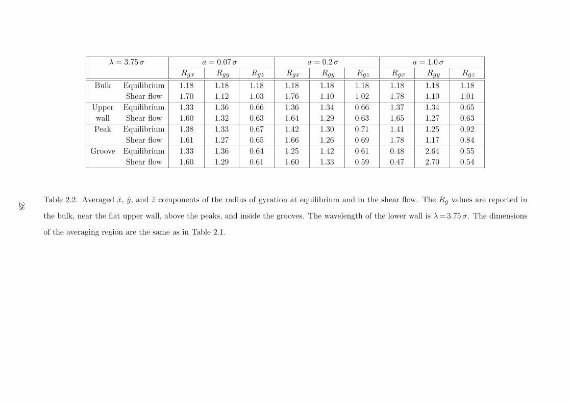
2.1 Averaged x , y , and z components of the radius of gyration at equilibrium and in the shear flow. The gR values are reported in the bulk, near the flat upper wall, above the peaks, and inside the grooves. The wavelength of the lower wall is 7.5λ σ= . The size of the averaging region above the peaks and inside the grooves is 12.5 1.5σ σ σ× × . The estimate of the error bars is 0.03σ . . . . . . . . . . . . . . . . . . . . . . . . . . . . . . . . . . . . . . . . . . . . . . . . . . . . . . . . . . . 27 2.2 Averaged x , y , and z components of the radius of gyration at equilibrium and in the shear flow. The gR values are reported in the bulk, near the flat upper wall, above the peaks, and inside the grooves. The wavelength of the lower is 3.75λ σ= . The dimensions of the averaging region are the same as in the Table 2.1. . . . . . . . . . . . . . . . . . . . . . . . . . . . . . . . . . . . . . . . . . . . . . . . . . . . 28 3.1 The fluid pressure P at equilibrium, i.e., with the stationary upper wall, and

the channel height h (defined as a distance between the inner FCC planes) as a function of the fluid density. . . . . . . . . . . . . . . . . . . . . . . . . . . . . . . . . . . . . . 34

vi

LIST OF FIGURES

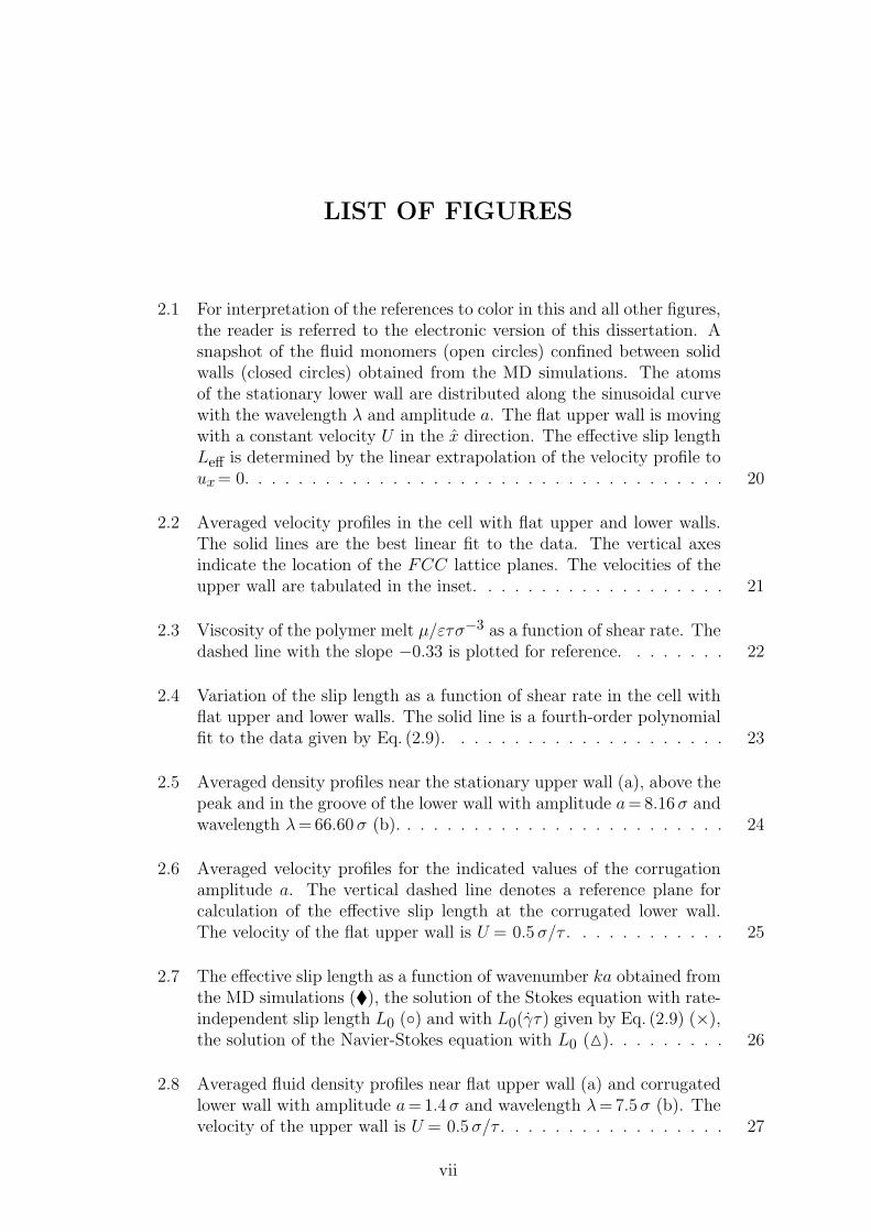
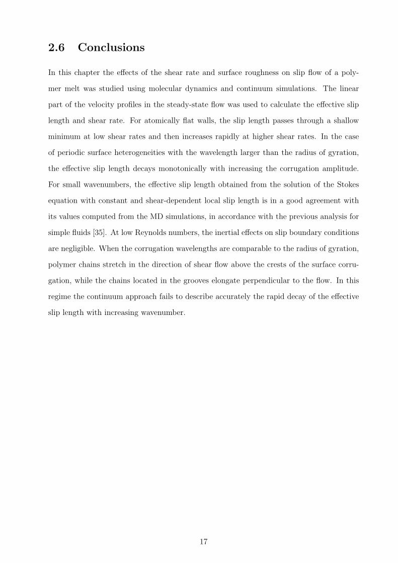
2.1 For interpretation of the references to color in this and all other figures,the reader is referred to the electronic version of this dissertation. Asnapshot of the fluid monomers (open circles) confined between solidwalls (closed circles) obtained from the MD simulations. The atomsof the stationary lower wall are distributed along the sinusoidal curvewith the wavelength λ and amplitude a. The flat upper wall is movingwith a constant velocity U in the x direction. The effective slip lengthLeff is determined by the linear extrapolation of the velocity profile toux = 0. . . . . . . . . . . . . . . . . . . . . . . . . . . . . . . . . . . . 20

2.2 Averaged velocity profiles in the cell with flat upper and lower walls.The solid lines are the best linear fit to the data. The vertical axesindicate the location of the FCC lattice planes. The velocities of theupper wall are tabulated in the inset. . . . . . . . . . . . . . . . . . . 21

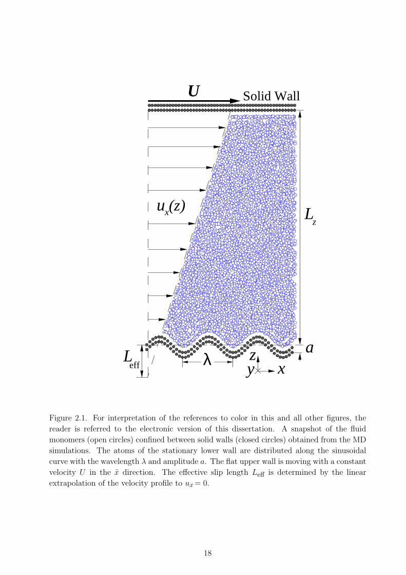
2.3 Viscosity of the polymer melt µ/ετσ−3 as a function of shear rate. Thedashed line with the slope −0.33 is plotted for reference. . . . . . . . 22

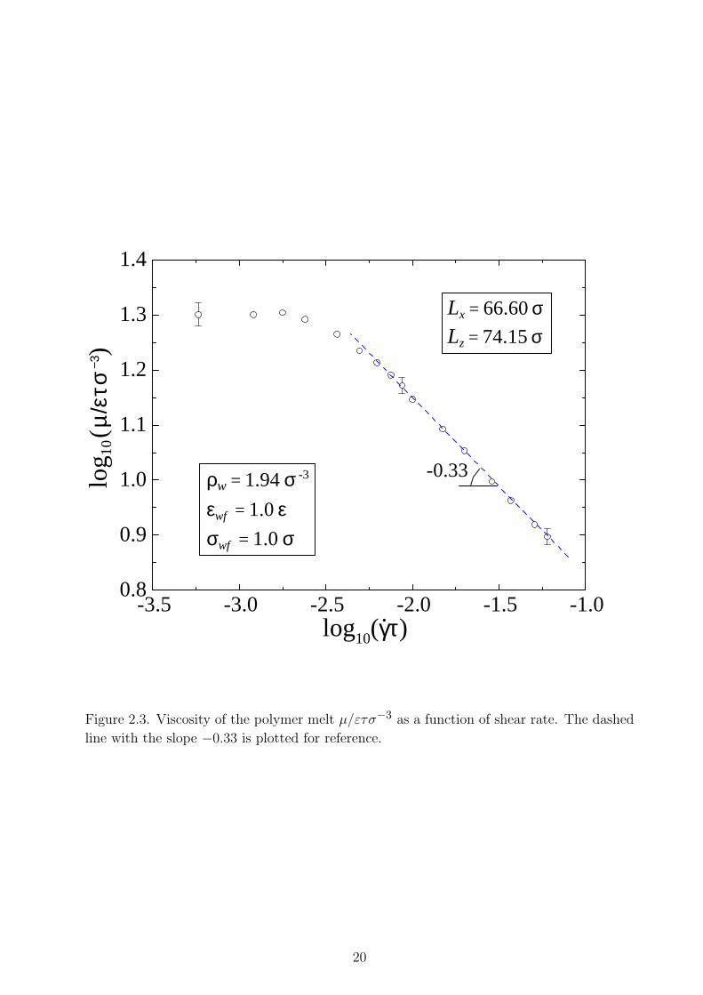
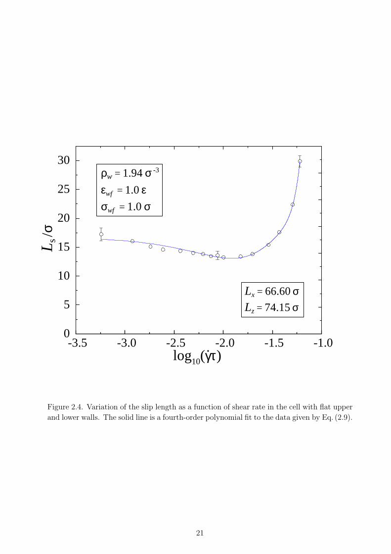
2.4 Variation of the slip length as a function of shear rate in the cell withflat upper and lower walls. The solid line is a fourth-order polynomialfit to the data given by Eq. (2.9). . . . . . . . . . . . . . . . . . . . . 23

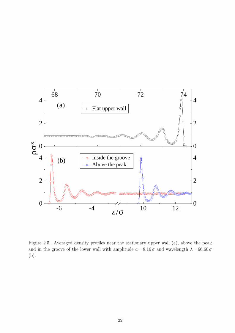
2.5 Averaged density profiles near the stationary upper wall (a), above thepeak and in the groove of the lower wall with amplitude a = 8.16 σ andwavelength λ = 66.60 σ (b). . . . . . . . . . . . . . . . . . . . . . . . . 24

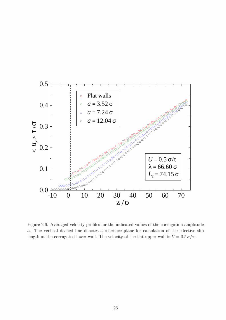
2.6 Averaged velocity profiles for the indicated values of the corrugationamplitude a. The vertical dashed line denotes a reference plane forcalculation of the effective slip length at the corrugated lower wall.The velocity of the flat upper wall is U = 0.5 σ/τ . . . . . . . . . . . . 25

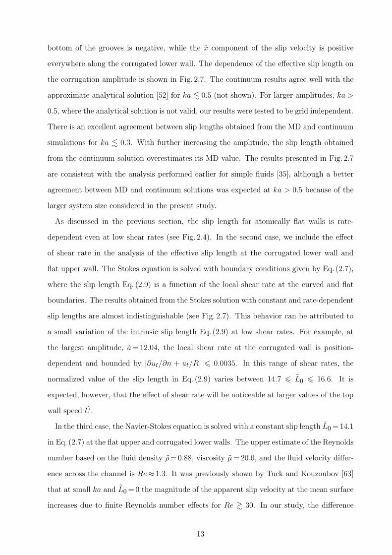
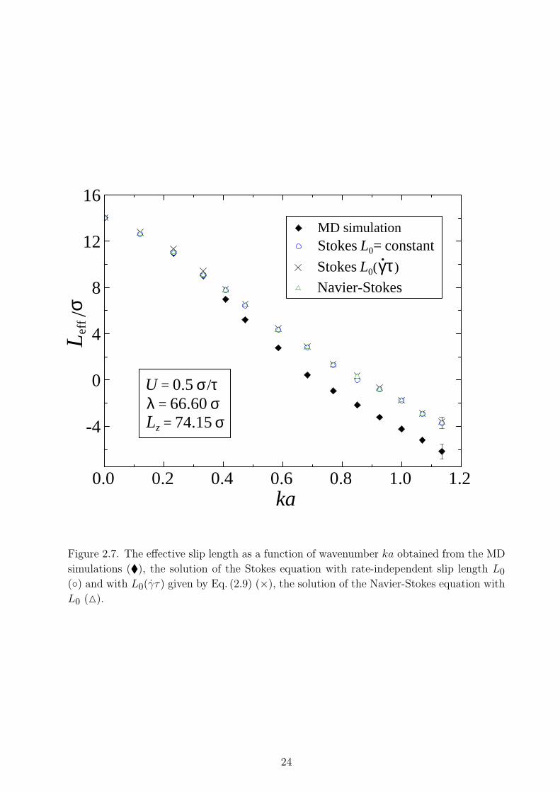
2.7 The effective slip length as a function of wavenumber ka obtained fromthe MD simulations (¨), the solution of the Stokes equation with rate-independent slip length L0 () and with L0(γτ) given by Eq. (2.9) (×),the solution of the Navier-Stokes equation with L0 (M). . . . . . . . . 26

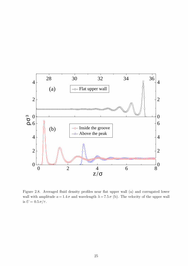
2.8 Averaged fluid density profiles near flat upper wall (a) and corrugatedlower wall with amplitude a = 1.4 σ and wavelength λ = 7.5 σ (b). Thevelocity of the upper wall is U = 0.5 σ/τ . . . . . . . . . . . . . . . . . 27

vii

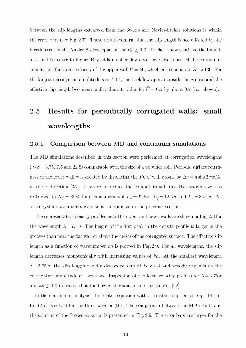
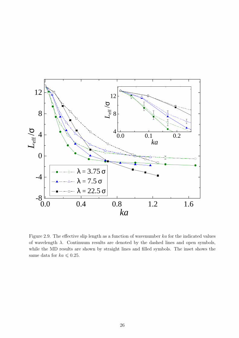
2.9 The effective slip length as a function of wavenumber ka for the indi-cated values of wavelength λ. Continuum results are denoted by thedashed lines and open symbols, while the MD results are shown bystraight lines and filled symbols. The inset shows the same data forka 6 0.25. . . . . . . . . . . . . . . . . . . . . . . . . . . . . . . . . . 28

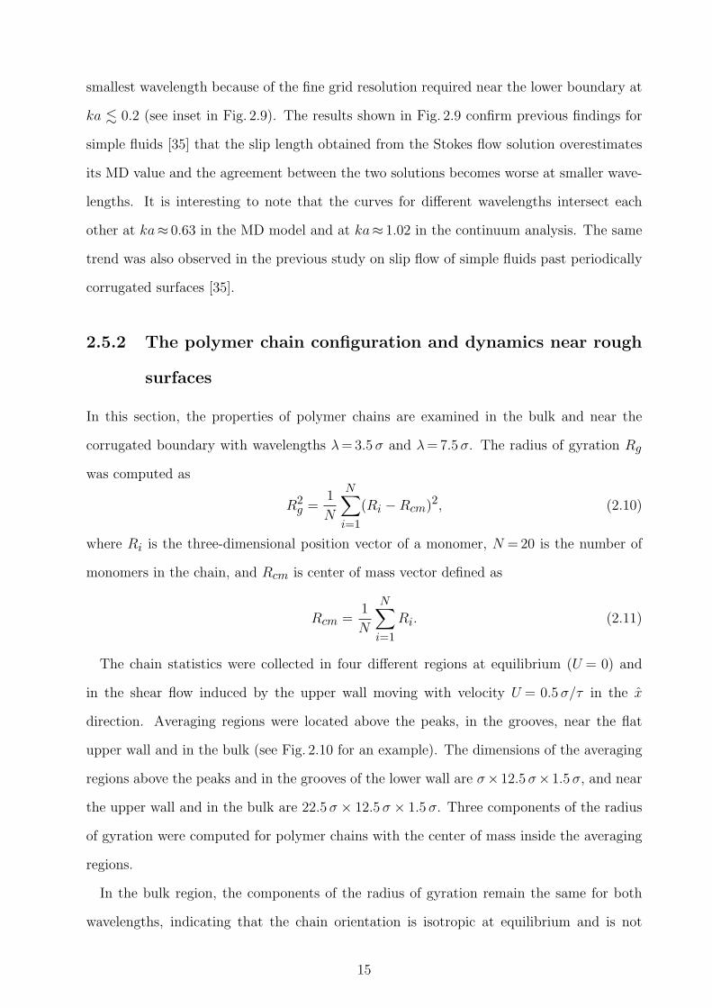
2.10 A snapshot of four polymer chains near the lower corrugated wall forwavelength λ = 7.5 σ and amplitude a = 1.4 σ. The velocity of theupper wall is U = 0.5 σ/τ . . . . . . . . . . . . . . . . . . . . . . . . . 29

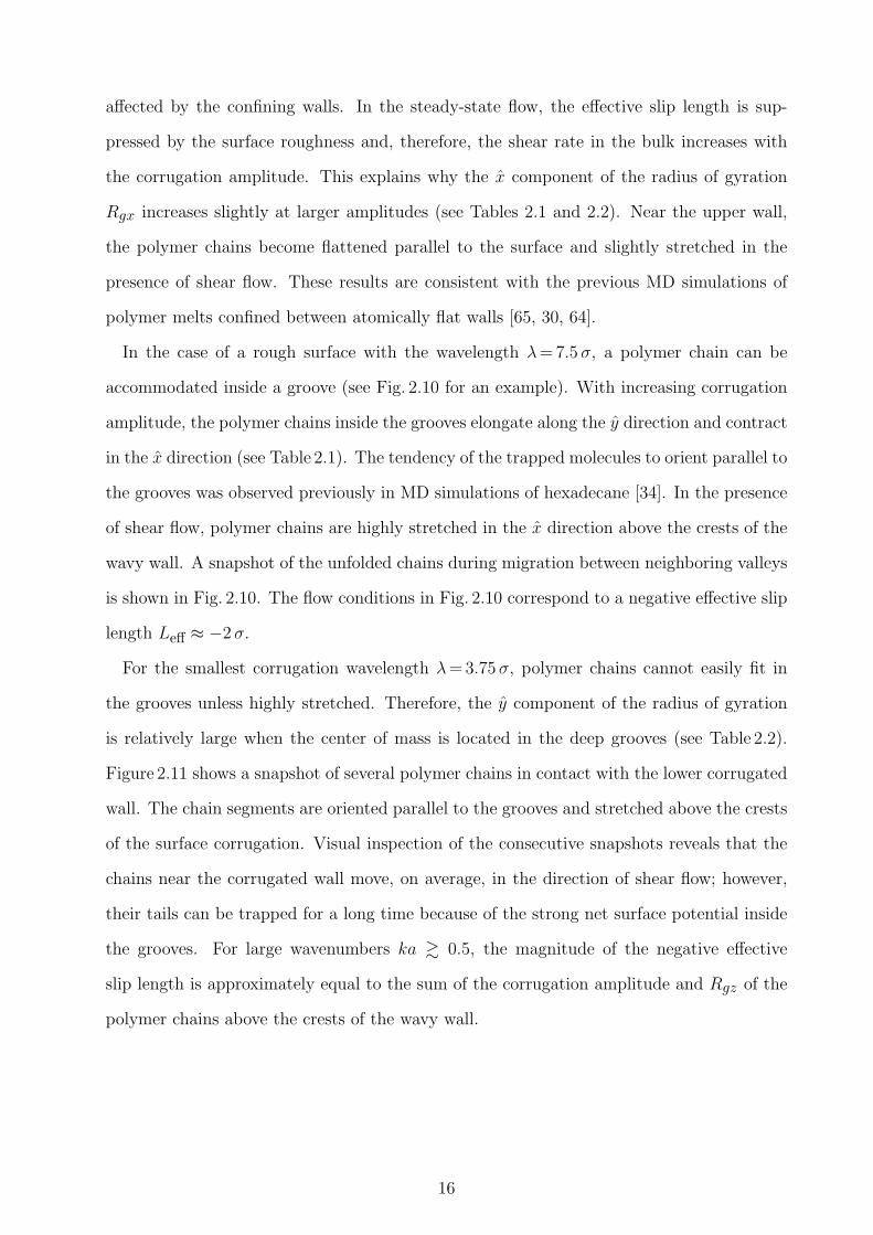
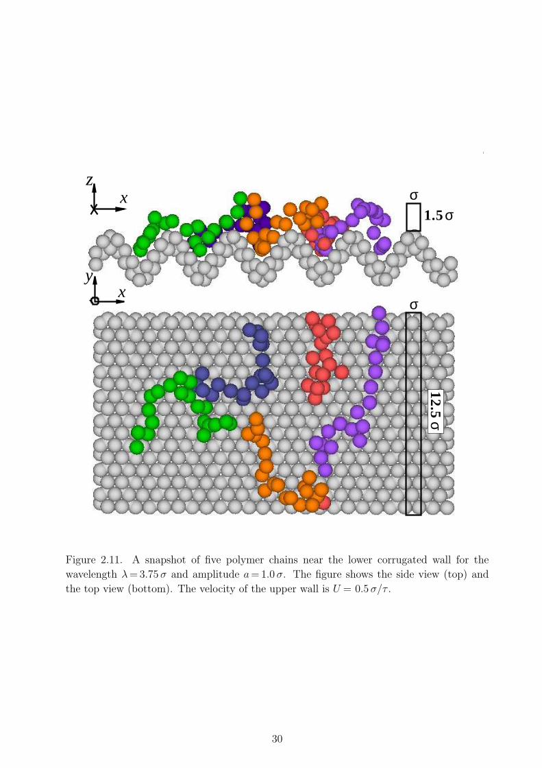
2.11 A snapshot of five polymer chains near the lower corrugated wall forthe wavelength λ = 3.75 σ and amplitude a = 1.0 σ. The figure showsthe side view (top) and the top view (bottom). The velocity of theupper wall is U = 0.5 σ/τ . . . . . . . . . . . . . . . . . . . . . . . . . 30

3.1 A schematic representation of the steady-state shear flow in the Cou-ette cell. The upper wall is translated with a constant velocity U inthe x direction. The fluid slip velocity is determined from the relationVs = γLs, where γ is the slope of the velocity profile and Ls is the sliplength. . . . . . . . . . . . . . . . . . . . . . . . . . . . . . . . . . . . 43

3.2 Averaged fluid density profiles near the stationary thermal wall withκ = 1200 ε/σ2 and εwf/ε = 0.9. The velocities of the upper wall aretabulated in the inset. The fluid density in the center of the cell isρ = 0.91 σ−3. The left vertical axis denotes the position of the liq-uid/solid interface at z = − 14.74 σ. . . . . . . . . . . . . . . . . . . . 44

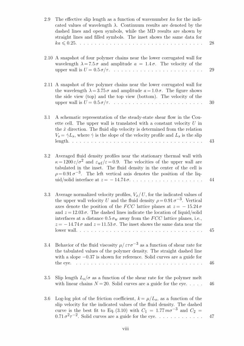
3.3 Average normalized velocity profiles, Vx/U , for the indicated values ofthe upper wall velocity U and the fluid density ρ = 0.91 σ−3. Verticalaxes denote the position of the FCC lattice planes at z = − 15.24 σand z = 12.03 σ. The dashed lines indicate the location of liquid/solidinterfaces at a distance 0.5 σw away from the FCC lattice planes, i.e.,z = − 14.74 σ and z = 11.53 σ. The inset shows the same data near thelower wall. . . . . . . . . . . . . . . . . . . . . . . . . . . . . . . . . . 45

3.4 Behavior of the fluid viscosity µ/ ετσ−3 as a function of shear rate forthe tabulated values of the polymer density. The straight dashed linewith a slope −0.37 is shown for reference. Solid curves are a guide forthe eye. . . . . . . . . . . . . . . . . . . . . . . . . . . . . . . . . . . 46

3.5 Slip length Ls/σ as a function of the shear rate for the polymer meltwith linear chains N = 20. Solid curves are a guide for the eye. . . . . 46

3.6 Log-log plot of the friction coefficient, k = µ/Ls, as a function of theslip velocity for the indicated values of the fluid density. The dashedcurve is the best fit to Eq. (3.10) with C1 = 1.77 mσ−3 and C2 =0.71 σ2τ−2. Solid curves are a guide for the eye. . . . . . . . . . . . . 47

viii

3.7 Master curve for the friction coefficient as a function of the slip velocity.The same data as in Fig. 3.6. The values of the friction coefficientk∗ [ ετσ−4] and the slip velocity V ∗s [ σ/τ ] used for normalization ofthe data are shown in the inset. The dashed line y = [1 + (4x)2]−0.35

is plotted for reference. . . . . . . . . . . . . . . . . . . . . . . . . . . 48

3.8 Structure factor S(kx, ky) in the first fluid layer for the fluid den-

sity ρ = 0.91 σ−3. The upper wall velocity is U = 0.05 σ/τ (a) andU = 5.0 σ/τ (b). The same flow conditions as in Fig. 3.3. . . . . . . . 49

3.9 Temperature profiles for the indicated values of the upper wall speedU and the fluid density ρ = 0.91 σ−3. Vertical dashed lines denote theposition of the liquid/solid interface. The inset shows the x, y and zcomponents of the temperature profile near the stationary lower wallwhen the velocity of the upper wall is U = 5.0 σ/τ . . . . . . . . . . . 50

3.10 Log-log plot of Ls/µ as a function of the ratio T1kB/ε [S(G1) ρc σ3]−1

for the indicated values of the polymer density. The solid line with aslope 0.9 is plotted for reference. . . . . . . . . . . . . . . . . . . . . . 51

3.11 Log-log plot of the ratio Ls/µ as a function of the variable S(0)/ [S(G1) ρc σ3].The values of the fluid density are tabulated in the inset. The samedata as in Fig. 3.10. The straight solid line with a slope 1.15 is plottedas a reference. . . . . . . . . . . . . . . . . . . . . . . . . . . . . . . . 52

4.1 Schematic diagram of the steady-state Couette flow over a rough sur-face. The upper flat wall is moving with a constant velocity U in thex direction. The lower stationary wall is modeled as a sinusoidal wavewith amplitude a and wavelength λ. The wavenumber ka = 2 πa/λvaries in the range 0 6 ka 6 1.26. . . . . . . . . . . . . . . . . . . . . 68

4.2 Diagram of a bilinear element in (a) the physical coordinate system(x, z) and (b) a transformed element in the natural coordinate system(ξ, η). . . . . . . . . . . . . . . . . . . . . . . . . . . . . . . . . . . . 68

4.3 The effective slip length as a function of wavenumber ka computedfrom the solution of the Stokes equation with the no-slip boundarycondition. The primary vortex is formed at the bottom of the valleyfor ka > 0.79 (see the vertical arrow at ka = 0.79). The solid line iscalculated using Eq. (4.18). The inset shows the normalized velocityprofiles obtained from the Stokes solution for the selected values of ka.The dashed line located at a = 0 is the reference for calculating theeffective slip length. . . . . . . . . . . . . . . . . . . . . . . . . . . . . 69

4.4 Shear stress along the lower wavy wall computed from the Stokes solu-tion with no-slip boundary condition (L0 = 0) for the indicated valuesof wavenumber ka. The value τ∗w used for normalization is the shearstress at the flat wall. The intersection of the curves with the dashedline determines the location of the flow separation and attachment in-side the valley. . . . . . . . . . . . . . . . . . . . . . . . . . . . . . . . 70

ix

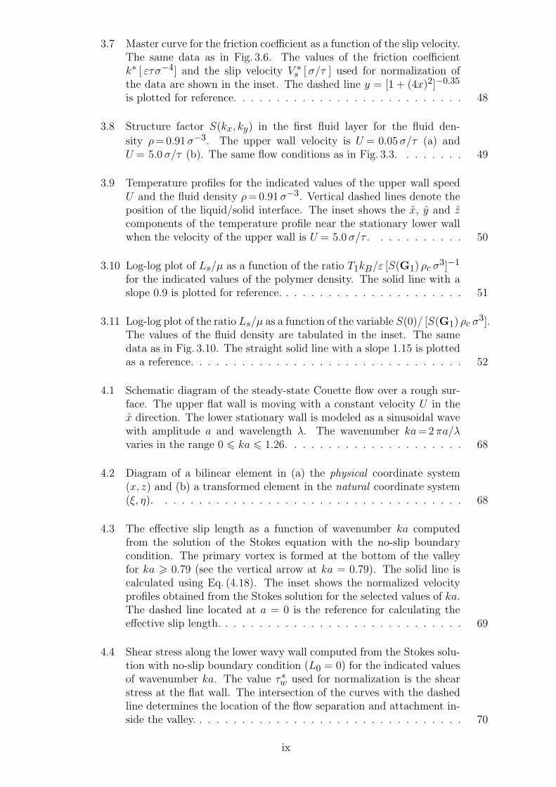
4.5 The normalized pressure along the lower corrugated boundary ex-tracted from the Stokes solution with no-slip boundary condition forthe same values of ka as in Fig. 4.4. The maximum pressure P ∗ forka = 1.12 and L0 = 0 is located in the bulk region at (x/λ, z/λ) '(0.07, 0.23). . . . . . . . . . . . . . . . . . . . . . . . . . . . . . . . . 71

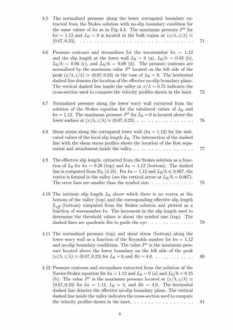
4.6 Pressure contours and streamlines for the wavenumber ka = 1.12and the slip length at the lower wall L0 = 0 (a), L0/h = 0.03 (b),L0/h = 0.06 (c), and L0/h = 0.08 (d). The pressure contours arenormalized by the maximum value P ∗ located on the left side of thepeak (x/λ, z/λ) ' (0.07, 0.23) in the case of L0 = 0. The horizontaldashed line denotes the location of the effective no-slip boundary plane.The vertical dashed line inside the valley at x/λ = 0.75 indicates thecross-section used to compute the velocity profiles shown in the inset. 72

4.7 Normalized pressure along the lower wavy wall extracted from thesolution of the Stokes equation for the tabulated values of L0 andka = 1.12. The maximum pressure P ∗ for L0 = 0 is located above thelower surface at (x/λ, z/λ) ' (0.07, 0.23). . . . . . . . . . . . . . . . . 76

4.8 Shear stress along the corrugated lower wall (ka = 1.12) for the indi-cated values of the local slip length L0. The intersection of the dashedline with the shear stress profiles shows the location of the flow sepa-ration and attachment inside the valley. . . . . . . . . . . . . . . . . . 77

4.9 The effective slip length, extracted from the Stokes solution as a func-tion of L0 for ka = 0.28 (top) and ka = 1.12 (bottom). The dashedline is computed from Eq. (4.18). For ka = 1.12 and L0/h 6 0.067, thevortex is formed in the valley (see the vertical arrow at L0/h = 0.067).The error bars are smaller than the symbol size. . . . . . . . . . . . . 78

4.10 The intrinsic slip length L0 above which there is no vortex at thebottom of the valley (top) and the corresponding effective slip lengthLeff (bottom) computed from the Stokes solution and plotted as afunction of wavenumber ka. The increment in the slip length used todetermine the threshold values is about the symbol size (top). Thedashed lines are quadratic fits to guide the eye. . . . . . . . . . . . . 79

4.11 The normalized pressure (top) and shear stress (bottom) along thelower wavy wall as a function of the Reynolds number for ka = 1.12and no-slip boundary conditions. The value P ∗ is the maximum pres-sure located above the lower boundary on the left side of the peak(x/λ, z/λ) ' (0.07, 0.23) for L0 = 0 and Re = 4.0. . . . . . . . . . . . 80

4.12 Pressure contours and streamlines extracted from the solution of theNavier-Stokes equation for ka = 1.12 and L0 = 0 (a) and L0/h = 0.25(b). The value P ∗ is the maximum pressure located at (x/λ, z/λ) '(0.07, 0.23) for ka = 1.12, L0 = 0, and Re = 4.0. The horizontaldashed line denotes the effective no-slip boundary plane. The verticaldashed line inside the valley indicates the cross-section used to computethe velocity profiles shown in the inset. . . . . . . . . . . . . . . . . . 81

x

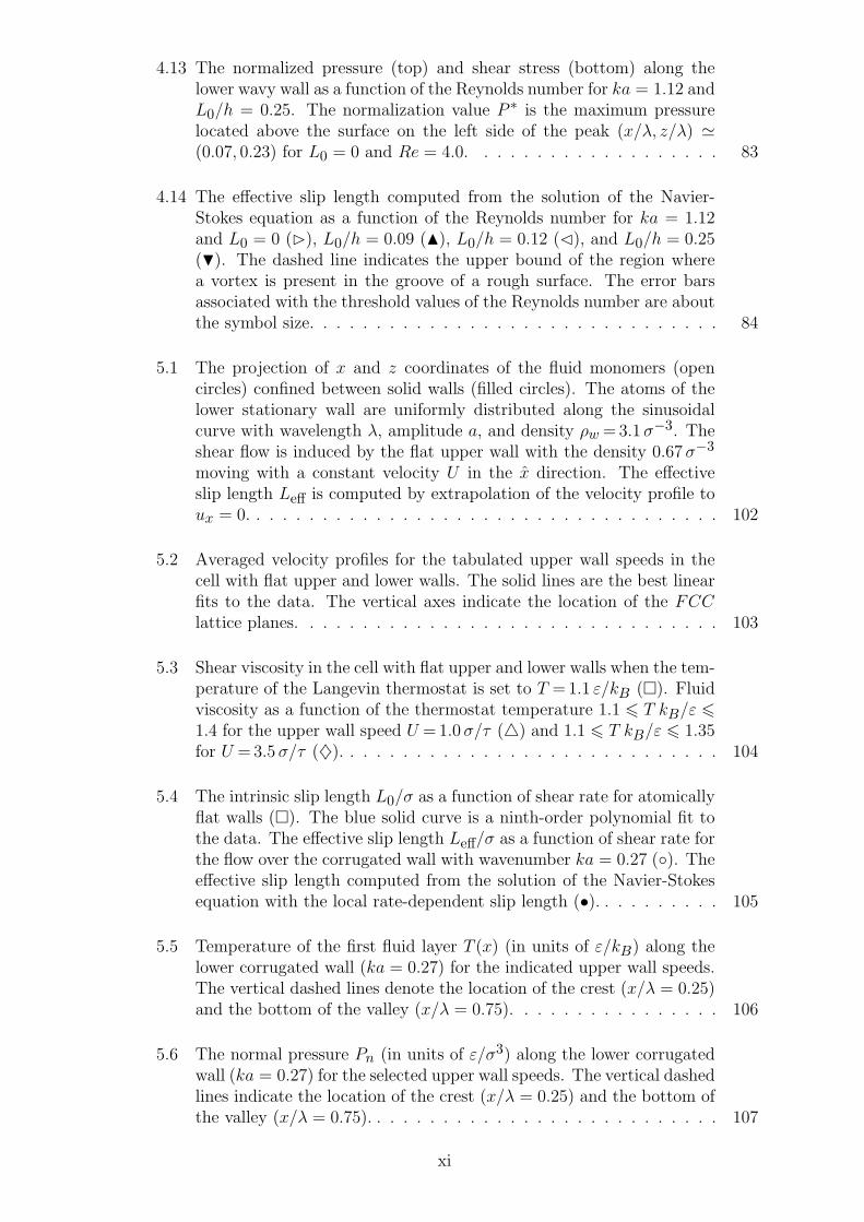
4.13 The normalized pressure (top) and shear stress (bottom) along thelower wavy wall as a function of the Reynolds number for ka = 1.12 andL0/h = 0.25. The normalization value P ∗ is the maximum pressurelocated above the surface on the left side of the peak (x/λ, z/λ) '(0.07, 0.23) for L0 = 0 and Re = 4.0. . . . . . . . . . . . . . . . . . . 83

4.14 The effective slip length computed from the solution of the Navier-Stokes equation as a function of the Reynolds number for ka = 1.12and L0 = 0 (B), L0/h = 0.09 (N), L0/h = 0.12 (C), and L0/h = 0.25(H). The dashed line indicates the upper bound of the region wherea vortex is present in the groove of a rough surface. The error barsassociated with the threshold values of the Reynolds number are aboutthe symbol size. . . . . . . . . . . . . . . . . . . . . . . . . . . . . . . 84

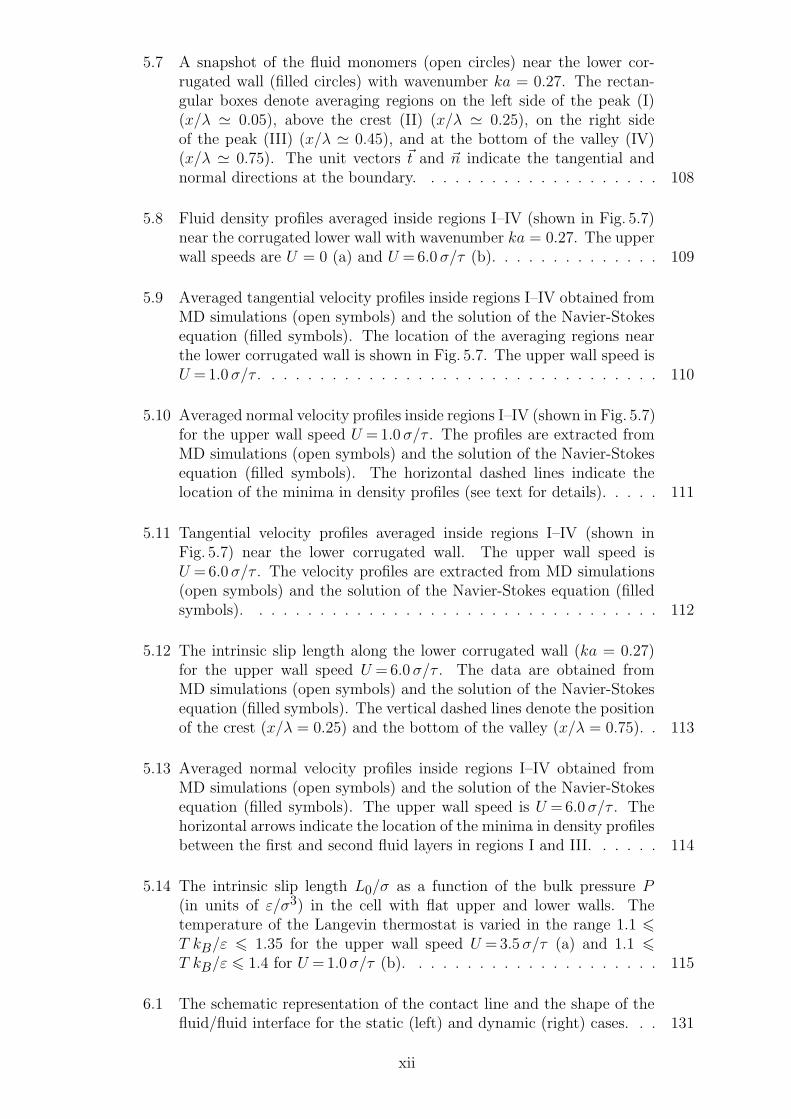
5.1 The projection of x and z coordinates of the fluid monomers (opencircles) confined between solid walls (filled circles). The atoms of thelower stationary wall are uniformly distributed along the sinusoidalcurve with wavelength λ, amplitude a, and density ρw = 3.1 σ−3. Theshear flow is induced by the flat upper wall with the density 0.67 σ−3

moving with a constant velocity U in the x direction. The effectiveslip length Leff is computed by extrapolation of the velocity profile toux = 0. . . . . . . . . . . . . . . . . . . . . . . . . . . . . . . . . . . . 102

5.2 Averaged velocity profiles for the tabulated upper wall speeds in thecell with flat upper and lower walls. The solid lines are the best linearfits to the data. The vertical axes indicate the location of the FCClattice planes. . . . . . . . . . . . . . . . . . . . . . . . . . . . . . . . 103

5.3 Shear viscosity in the cell with flat upper and lower walls when the tem-perature of the Langevin thermostat is set to T = 1.1 ε/kB (¤). Fluidviscosity as a function of the thermostat temperature 1.1 6 T kB/ε 61.4 for the upper wall speed U = 1.0 σ/τ (4) and 1.1 6 T kB/ε 6 1.35for U = 3.5 σ/τ (♦). . . . . . . . . . . . . . . . . . . . . . . . . . . . . 104

5.4 The intrinsic slip length L0/σ as a function of shear rate for atomicallyflat walls (¤). The blue solid curve is a ninth-order polynomial fit tothe data. The effective slip length Leff/σ as a function of shear rate forthe flow over the corrugated wall with wavenumber ka = 0.27 (). Theeffective slip length computed from the solution of the Navier-Stokesequation with the local rate-dependent slip length (•). . . . . . . . . . 105

5.5 Temperature of the first fluid layer T (x) (in units of ε/kB) along thelower corrugated wall (ka = 0.27) for the indicated upper wall speeds.The vertical dashed lines denote the location of the crest (x/λ = 0.25)and the bottom of the valley (x/λ = 0.75). . . . . . . . . . . . . . . . 106

5.6 The normal pressure Pn (in units of ε/σ3) along the lower corrugatedwall (ka = 0.27) for the selected upper wall speeds. The vertical dashedlines indicate the location of the crest (x/λ = 0.25) and the bottom ofthe valley (x/λ = 0.75). . . . . . . . . . . . . . . . . . . . . . . . . . . 107

xi

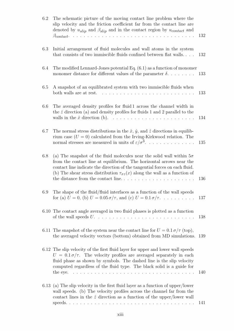
5.7 A snapshot of the fluid monomers (open circles) near the lower cor-rugated wall (filled circles) with wavenumber ka = 0.27. The rectan-gular boxes denote averaging regions on the left side of the peak (I)(x/λ ' 0.05), above the crest (II) (x/λ ' 0.25), on the right sideof the peak (III) (x/λ ' 0.45), and at the bottom of the valley (IV)(x/λ ' 0.75). The unit vectors ~t and ~n indicate the tangential andnormal directions at the boundary. . . . . . . . . . . . . . . . . . . . 108

5.8 Fluid density profiles averaged inside regions I–IV (shown in Fig. 5.7)near the corrugated lower wall with wavenumber ka = 0.27. The upperwall speeds are U = 0 (a) and U = 6.0 σ/τ (b). . . . . . . . . . . . . . 109

5.9 Averaged tangential velocity profiles inside regions I–IV obtained fromMD simulations (open symbols) and the solution of the Navier-Stokesequation (filled symbols). The location of the averaging regions nearthe lower corrugated wall is shown in Fig. 5.7. The upper wall speed isU = 1.0 σ/τ . . . . . . . . . . . . . . . . . . . . . . . . . . . . . . . . . 110

5.10 Averaged normal velocity profiles inside regions I–IV (shown in Fig. 5.7)for the upper wall speed U = 1.0 σ/τ . The profiles are extracted fromMD simulations (open symbols) and the solution of the Navier-Stokesequation (filled symbols). The horizontal dashed lines indicate thelocation of the minima in density profiles (see text for details). . . . . 111

5.11 Tangential velocity profiles averaged inside regions I–IV (shown inFig. 5.7) near the lower corrugated wall. The upper wall speed isU = 6.0 σ/τ . The velocity profiles are extracted from MD simulations(open symbols) and the solution of the Navier-Stokes equation (filledsymbols). . . . . . . . . . . . . . . . . . . . . . . . . . . . . . . . . . 112

5.12 The intrinsic slip length along the lower corrugated wall (ka = 0.27)for the upper wall speed U = 6.0 σ/τ . The data are obtained fromMD simulations (open symbols) and the solution of the Navier-Stokesequation (filled symbols). The vertical dashed lines denote the positionof the crest (x/λ = 0.25) and the bottom of the valley (x/λ = 0.75). . 113

5.13 Averaged normal velocity profiles inside regions I–IV obtained fromMD simulations (open symbols) and the solution of the Navier-Stokesequation (filled symbols). The upper wall speed is U = 6.0 σ/τ . Thehorizontal arrows indicate the location of the minima in density profilesbetween the first and second fluid layers in regions I and III. . . . . . 114

5.14 The intrinsic slip length L0/σ as a function of the bulk pressure P(in units of ε/σ3) in the cell with flat upper and lower walls. Thetemperature of the Langevin thermostat is varied in the range 1.1 6T kB/ε 6 1.35 for the upper wall speed U = 3.5 σ/τ (a) and 1.1 6T kB/ε 6 1.4 for U = 1.0 σ/τ (b). . . . . . . . . . . . . . . . . . . . . 115

6.1 The schematic representation of the contact line and the shape of thefluid/fluid interface for the static (left) and dynamic (right) cases. . . 131

xii

6.2 The schematic picture of the moving contact line problem where theslip velocity and the friction coefficient far from the contact line aredenoted by uslip and βslip and in the contact region by ucontact andβcontact. . . . . . . . . . . . . . . . . . . . . . . . . . . . . . . . . . . 132

6.3 Initial arrangement of fluid molecules and wall atoms in the systemthat consists of two immiscible fluids confined between flat walls. . . . 132

6.4 The modified Lennard-Jones potential Eq. (6.1) as a function of monomermonomer distance for different values of the parameter δ. . . . . . . . 133

6.5 A snapshot of an equilibrated system with two immiscible fluids whenboth walls are at rest. . . . . . . . . . . . . . . . . . . . . . . . . . . 133

6.6 The averaged density profiles for fluid 1 across the channel width inthe z direction (a) and density profiles for fluids 1 and 2 parallel to thewalls in the x direction (b). . . . . . . . . . . . . . . . . . . . . . . . 134

6.7 The normal stress distributions in the x, y, and z directions in equilib-rium case (U = 0) calculated from the Irving-Kirkwood relation. Thenormal stresses are measured in units of ε/σ3. . . . . . . . . . . . . . 135

6.8 (a) The snapshot of the fluid molecules near the solid wall within 5σfrom the contact line at equilibrium. The horizontal arrows near thecontact line indicate the direction of the tangential forces on each fluid.(b) The shear stress distribution τxz(x) along the wall as a function ofthe distance from the contact line. . . . . . . . . . . . . . . . . . . . . 136

6.9 The shape of the fluid/fluid interfaces as a function of the wall speedsfor (a) U = 0, (b) U = 0.05 σ/τ , and (c) U = 0.1 σ/τ . . . . . . . . . . 137

6.10 The contact angle averaged in two fluid phases is plotted as a functionof the wall speeds U . . . . . . . . . . . . . . . . . . . . . . . . . . . . 138

6.11 The snapshot of the system near the contact line for U = 0.1 σ/τ (top),the averaged velocity vectors (bottom) obtained from MD simulations. 139

6.12 The slip velocity of the first fluid layer for upper and lower wall speedsU = 0.1 σ/τ . The velocity profiles are averaged separately in eachfluid phase as shown by symbols. The dashed line is the slip velocitycomputed regardless of the fluid type. The black solid is a guide forthe eye. . . . . . . . . . . . . . . . . . . . . . . . . . . . . . . . . . . 140

6.13 (a) The slip velocity in the first fluid layer as a function of upper/lowerwall speeds. (b) The velocity profiles across the channel far from thecontact lines in the z direction as a function of the upper/lower wallspeeds. . . . . . . . . . . . . . . . . . . . . . . . . . . . . . . . . . . . 141

xiii

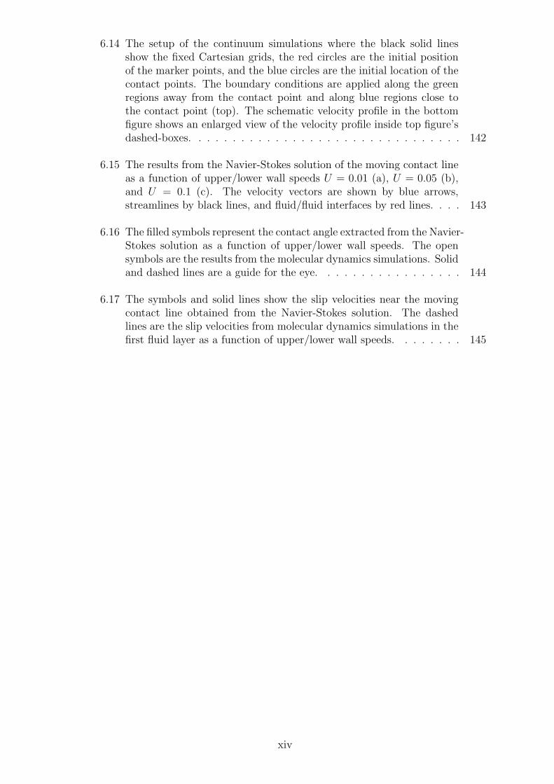
6.14 The setup of the continuum simulations where the black solid linesshow the fixed Cartesian grids, the red circles are the initial positionof the marker points, and the blue circles are the initial location of thecontact points. The boundary conditions are applied along the greenregions away from the contact point and along blue regions close tothe contact point (top). The schematic velocity profile in the bottomfigure shows an enlarged view of the velocity profile inside top figure’sdashed-boxes. . . . . . . . . . . . . . . . . . . . . . . . . . . . . . . . 142

6.15 The results from the Navier-Stokes solution of the moving contact lineas a function of upper/lower wall speeds U = 0.01 (a), U = 0.05 (b),and U = 0.1 (c). The velocity vectors are shown by blue arrows,streamlines by black lines, and fluid/fluid interfaces by red lines. . . . 143

6.16 The filled symbols represent the contact angle extracted from the Navier-Stokes solution as a function of upper/lower wall speeds. The opensymbols are the results from the molecular dynamics simulations. Solidand dashed lines are a guide for the eye. . . . . . . . . . . . . . . . . 144

6.17 The symbols and solid lines show the slip velocities near the movingcontact line obtained from the Navier-Stokes solution. The dashedlines are the slip velocities from molecular dynamics simulations in thefirst fluid layer as a function of upper/lower wall speeds. . . . . . . . 145

xiv

CHAPTER 1

Introduction

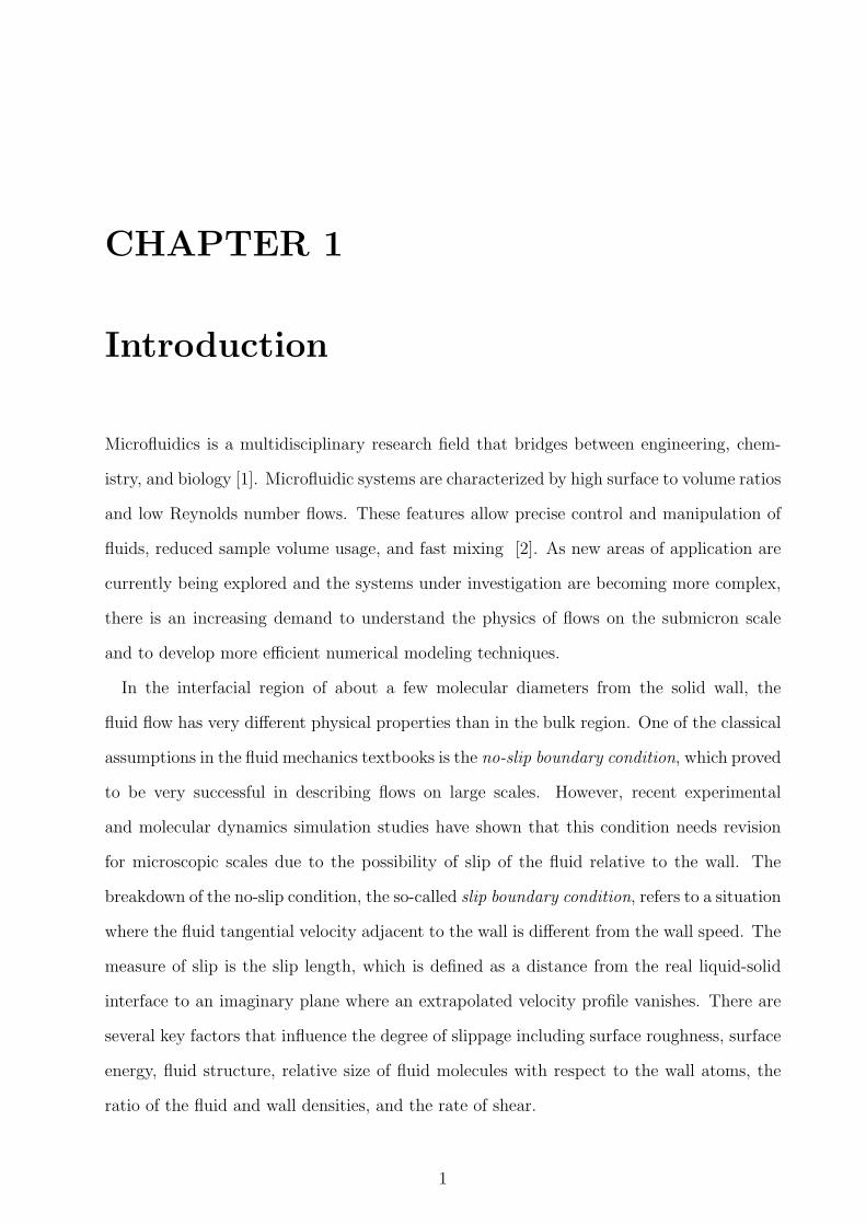
Microfluidics is a multidisciplinary research field that bridges between engineering, chem-

istry, and biology [1]. Microfluidic systems are characterized by high surface to volume ratios

and low Reynolds number flows. These features allow precise control and manipulation of

fluids, reduced sample volume usage, and fast mixing [2]. As new areas of application are

currently being explored and the systems under investigation are becoming more complex,

there is an increasing demand to understand the physics of flows on the submicron scale

and to develop more efficient numerical modeling techniques.

In the interfacial region of about a few molecular diameters from the solid wall, the

fluid flow has very different physical properties than in the bulk region. One of the classical

assumptions in the fluid mechanics textbooks is the no-slip boundary condition, which proved

to be very successful in describing flows on large scales. However, recent experimental

and molecular dynamics simulation studies have shown that this condition needs revision

for microscopic scales due to the possibility of slip of the fluid relative to the wall. The

breakdown of the no-slip condition, the so-called slip boundary condition, refers to a situation

where the fluid tangential velocity adjacent to the wall is different from the wall speed. The

measure of slip is the slip length, which is defined as a distance from the real liquid-solid

interface to an imaginary plane where an extrapolated velocity profile vanishes. There are

several key factors that influence the degree of slippage including surface roughness, surface

energy, fluid structure, relative size of fluid molecules with respect to the wall atoms, the

ratio of the fluid and wall densities, and the rate of shear.

1

In this dissertation, we investigate fluid flows and the slip phenomena in confined systems

using molecular dynamics (MD) and continuum simulations. The molecular dynamics tech-

nique, despite its computational cost, provides a detailed information about the structure,

dynamics, and thermodynamics of complex flows, especially near the solid/liquid interface.

On the other hand, the continuum modeling is computationally more affordable but requires

specification of the proper boundary conditions. One of the main themes in this dissertation

is a comparative analysis of fluid flows using both atomistic and continuum descriptions. In

particular, we numerically solve the Navier-Stokes equation for flows in various geometries

using the slip boundary conditions obtained from MD studies. The continuum predictions

are compared with the results of MD simulations for a wide range of parameters describing

liquid-solid interfaces, i.e., fluid structure (monatomic and polymeric liquids), wall struc-

ture (wall density and topological roughness), and flow conditions (low/high shear rates,

low/high Reynolds numbers, and single/two phase flows). The results are categorized as

follows.

In chapter II, molecular dynamics simulations are carried out to investigate the dynamic

behavior of the slip length for polymeric liquids confined between either atomically flat or

periodically corrugated surfaces. The MD results show that for atomically flat walls the

slip length depends non-linearly on shear rate. In contrast to the description of the flow

over smooth boundaries (with microscopic surface roughness) by the intrinsic slip length, it

is more appropriate to characterize the flow away from macroscopically rough surfaces by

the effective slip length, which is usually defined with respect to the location of the mean

roughness height. For periodically corrugated surfaces, the effective slip length gradually

decreases as a function of wavenumber. The polymer chain configuration and dynamics are

studied near rough surfaces. For flows over periodically corrugated surfaces, the solution

of the Stokes equation is compared with the results of MD simulations in a wide range of

wavelengths and amplitudes.

The effects of shear rate and fluid density on slip boundary conditions for polymer melt

flows past flat crystalline walls are investigated by molecular dynamics simulations in chapter

III. It is shown that the rate-dependent slip length exhibits a local minimum and then it

increases rapidly at higher shear rates. The friction coefficient at the liquid/solid interface

2

follows a power law decay as a function of the slip velocity. The ratio of the viscosity to the

slip length (i.e., friction coefficient at the liquid-solid interface) is determined by the surface

induced structure in the first fluid layer.

In chapter IV, we investigate the effects of local slip boundary conditions and the Reynolds

number on the flow structure near periodically corrugated surfaces and the effective slip

length. It was shown that for the Stokes flow with the local no-slip boundary condition, the

effective slip length decreases with increasing corrugation amplitude and a flow circulation

is developed in sufficiently deep grooves. The analysis of numerical solution of the Navier-

Stokes equation with the local slip condition shows that the inertial effects promote the

asymmetric vortex flow formation and reduce the effective slip length.

In chapter V, the slip flow of monatomic fluids over a periodically corrugated surface is

studied in a wide range of shear rates using molecular dynamics and continuum simula-

tions. The effective slip length in both methods is nearly constant at low shear rates and

it gradually increases at higher shear rates. The slight discrepancy between the effective

slip lengths computed from MD and continuum methods at high shear rates is explained

by careful examination of the local pressure, velocity, and density profiles along the wavy

surface.

The moving contact line problem is considered in the last chapter VI using molecular dy-

namics and continuum simulations. The MD simulations are carried out to resolve the flow

fields in the vicinity of the moving contact line at the molecular scale. Then, the bound-

ary conditions extracted from MD simulations is implemented in the continuum solution of

the Navier-Stokes equations (using finite difference/particle tracking methods) to reproduce

velocity profiles and the shape of the fluid/fluid interface.

3

CHAPTER 2

Rheological study of polymer flow

past rough surfaces with slip

boundary conditions

2.1 Introduction

The dynamics of fluid flow in confined geometries has gained renewed interest due to the

recent developments in micro- and nanofluidics [3]. The investigations are motivated by

important industrial applications including lubrication, coating, and painting processes.

The flow behavior at the sub-micron scale strongly depends on the boundary conditions at

the liquid/solid interface. A number of experimental studies on fluid flow past nonwetting

surfaces have shown that the conditions at the boundary deviate from the no-slip assump-

tion [4]. The most popular Navier model relates the slip velocity (the relative velocity of

the fluid with respect to the adjacent solid wall) and the shear rate with the proportionality

coefficient, the slip length, which is determined by the linear extrapolation of the fluid ve-

locity profile to zero. The magnitude of the slip length depends on several key parameters,

such as wettability [5, 6, 8, 7], surface roughness [9, 10, 11, 12, 13, 14], complex fluid struc-

ture [15, 16], and shear rate [17, 18, 19]. However, the experimental determination of the

slip length as a function of these parameters is hampered by the presence of several factors

with competing effects on the wall slip, e.g. surface roughness and wettability [9] or surface

4

roughness and shear rate [10].

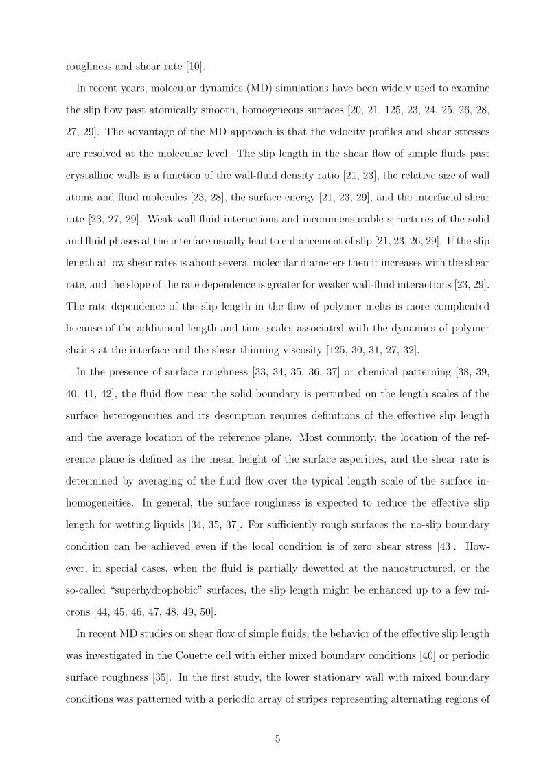
In recent years, molecular dynamics (MD) simulations have been widely used to examine

the slip flow past atomically smooth, homogeneous surfaces [20, 21, 125, 23, 24, 25, 26, 28,

27, 29]. The advantage of the MD approach is that the velocity profiles and shear stresses

are resolved at the molecular level. The slip length in the shear flow of simple fluids past

crystalline walls is a function of the wall-fluid density ratio [21, 23], the relative size of wall

atoms and fluid molecules [23, 28], the surface energy [21, 23, 29], and the interfacial shear

rate [23, 27, 29]. Weak wall-fluid interactions and incommensurable structures of the solid

and fluid phases at the interface usually lead to enhancement of slip [21, 23, 26, 29]. If the slip

length at low shear rates is about several molecular diameters then it increases with the shear

rate, and the slope of the rate dependence is greater for weaker wall-fluid interactions [23, 29].

The rate dependence of the slip length in the flow of polymer melts is more complicated

because of the additional length and time scales associated with the dynamics of polymer

chains at the interface and the shear thinning viscosity [125, 30, 31, 27, 32].

In the presence of surface roughness [33, 34, 35, 36, 37] or chemical patterning [38, 39,

40, 41, 42], the fluid flow near the solid boundary is perturbed on the length scales of the

surface heterogeneities and its description requires definitions of the effective slip length

and the average location of the reference plane. Most commonly, the location of the ref-

erence plane is defined as the mean height of the surface asperities, and the shear rate is

determined by averaging of the fluid flow over the typical length scale of the surface in-

homogeneities. In general, the surface roughness is expected to reduce the effective slip

length for wetting liquids [34, 35, 37]. For sufficiently rough surfaces the no-slip boundary

condition can be achieved even if the local condition is of zero shear stress [43]. How-

ever, in special cases, when the fluid is partially dewetted at the nanostructured, or the

so-called “superhydrophobic” surfaces, the slip length might be enhanced up to a few mi-

crons [44, 45, 46, 47, 48, 49, 50].

In recent MD studies on shear flow of simple fluids, the behavior of the effective slip length

was investigated in the Couette cell with either mixed boundary conditions [40] or periodic

surface roughness [35]. In the first study, the lower stationary wall with mixed boundary

conditions was patterned with a periodic array of stripes representing alternating regions of

5

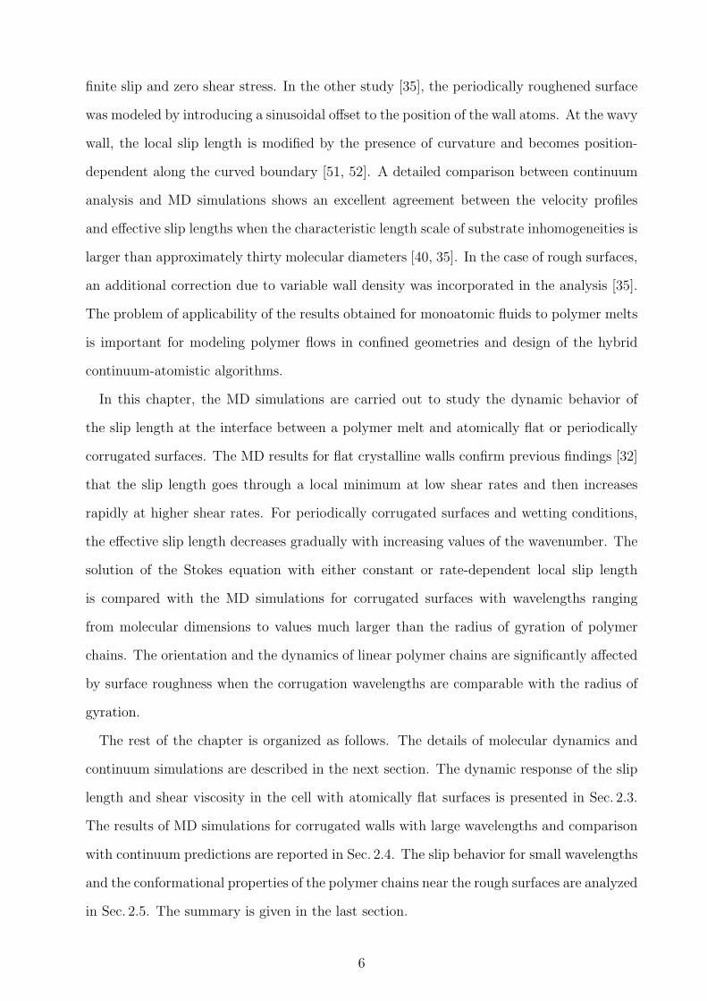
finite slip and zero shear stress. In the other study [35], the periodically roughened surface

was modeled by introducing a sinusoidal offset to the position of the wall atoms. At the wavy

wall, the local slip length is modified by the presence of curvature and becomes position-

dependent along the curved boundary [51, 52]. A detailed comparison between continuum

analysis and MD simulations shows an excellent agreement between the velocity profiles

and effective slip lengths when the characteristic length scale of substrate inhomogeneities is

larger than approximately thirty molecular diameters [40, 35]. In the case of rough surfaces,

an additional correction due to variable wall density was incorporated in the analysis [35].

The problem of applicability of the results obtained for monoatomic fluids to polymer melts

is important for modeling polymer flows in confined geometries and design of the hybrid

continuum-atomistic algorithms.

In this chapter, the MD simulations are carried out to study the dynamic behavior of

the slip length at the interface between a polymer melt and atomically flat or periodically

corrugated surfaces. The MD results for flat crystalline walls confirm previous findings [32]

that the slip length goes through a local minimum at low shear rates and then increases

rapidly at higher shear rates. For periodically corrugated surfaces and wetting conditions,

the effective slip length decreases gradually with increasing values of the wavenumber. The

solution of the Stokes equation with either constant or rate-dependent local slip length

is compared with the MD simulations for corrugated surfaces with wavelengths ranging

from molecular dimensions to values much larger than the radius of gyration of polymer

chains. The orientation and the dynamics of linear polymer chains are significantly affected

by surface roughness when the corrugation wavelengths are comparable with the radius of

gyration.

The rest of the chapter is organized as follows. The details of molecular dynamics and

continuum simulations are described in the next section. The dynamic response of the slip

length and shear viscosity in the cell with atomically flat surfaces is presented in Sec. 2.3.

The results of MD simulations for corrugated walls with large wavelengths and comparison

with continuum predictions are reported in Sec. 2.4. The slip behavior for small wavelengths

and the conformational properties of the polymer chains near the rough surfaces are analyzed

in Sec. 2.5. The summary is given in the last section.

6

2.2 The details of the numerical simulations

2.2.1 Molecular dynamics model

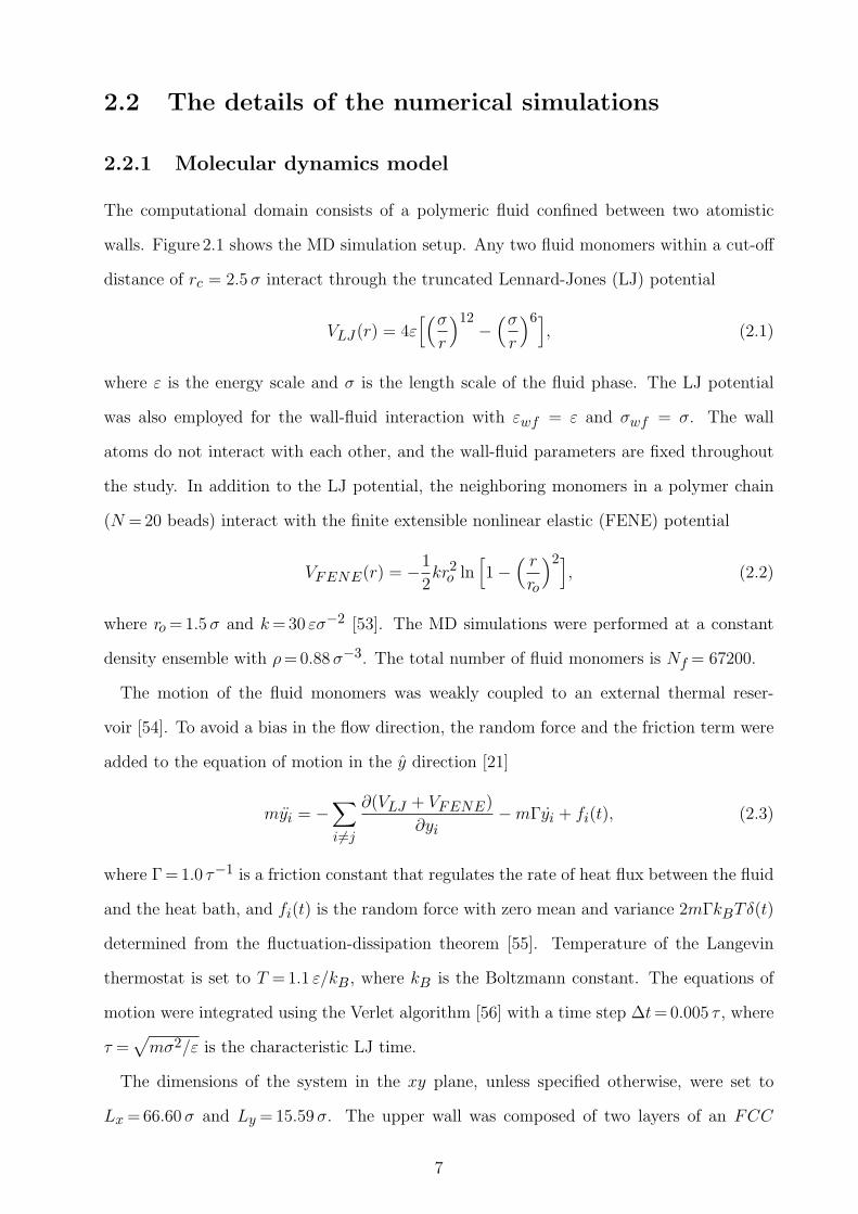
The computational domain consists of a polymeric fluid confined between two atomistic

walls. Figure 2.1 shows the MD simulation setup. Any two fluid monomers within a cut-off

distance of rc = 2.5 σ interact through the truncated Lennard-Jones (LJ) potential

VLJ (r) = 4ε[(σ

r

)12 −(σ

r

)6], (2.1)

where ε is the energy scale and σ is the length scale of the fluid phase. The LJ potential

was also employed for the wall-fluid interaction with εwf = ε and σwf = σ. The wall

atoms do not interact with each other, and the wall-fluid parameters are fixed throughout

the study. In addition to the LJ potential, the neighboring monomers in a polymer chain

(N = 20 beads) interact with the finite extensible nonlinear elastic (FENE) potential

VFENE(r) = −1

2kr2

o ln[1−

( r

ro

)2], (2.2)

where ro = 1.5 σ and k = 30 εσ−2 [53]. The MD simulations were performed at a constant

density ensemble with ρ = 0.88 σ−3. The total number of fluid monomers is Nf = 67200.

The motion of the fluid monomers was weakly coupled to an external thermal reser-

voir [54]. To avoid a bias in the flow direction, the random force and the friction term were

added to the equation of motion in the y direction [21]

myi = −∑

i6=j

∂(VLJ + VFENE)

∂yi−mΓyi + fi(t), (2.3)

where Γ = 1.0 τ−1 is a friction constant that regulates the rate of heat flux between the fluid

and the heat bath, and fi(t) is the random force with zero mean and variance 2mΓkBTδ(t)

determined from the fluctuation-dissipation theorem [55]. Temperature of the Langevin

thermostat is set to T = 1.1 ε/kB , where kB is the Boltzmann constant. The equations of

motion were integrated using the Verlet algorithm [56] with a time step ∆t = 0.005 τ , where

τ =√

mσ2/ε is the characteristic LJ time.

The dimensions of the system in the xy plane, unless specified otherwise, were set to

Lx = 66.60 σ and Ly = 15.59 σ. The upper wall was composed of two layers of an FCC

7

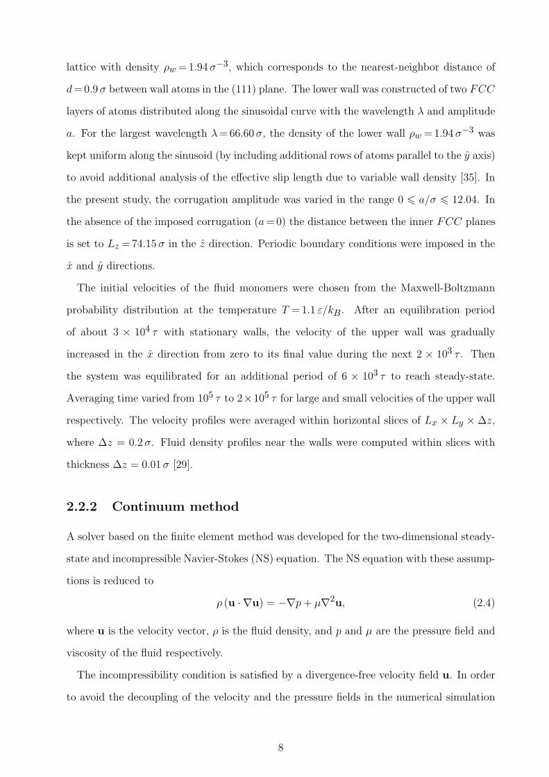
lattice with density ρw = 1.94 σ−3, which corresponds to the nearest-neighbor distance of

d = 0.9 σ between wall atoms in the (111) plane. The lower wall was constructed of two FCC

layers of atoms distributed along the sinusoidal curve with the wavelength λ and amplitude

a. For the largest wavelength λ = 66.60 σ, the density of the lower wall ρw = 1.94 σ−3 was

kept uniform along the sinusoid (by including additional rows of atoms parallel to the y axis)

to avoid additional analysis of the effective slip length due to variable wall density [35]. In

the present study, the corrugation amplitude was varied in the range 0 6 a/σ 6 12.04. In

the absence of the imposed corrugation (a = 0) the distance between the inner FCC planes

is set to Lz = 74.15 σ in the z direction. Periodic boundary conditions were imposed in the

x and y directions.

The initial velocities of the fluid monomers were chosen from the Maxwell-Boltzmann

probability distribution at the temperature T = 1.1 ε/kB . After an equilibration period

of about 3 × 104 τ with stationary walls, the velocity of the upper wall was gradually

increased in the x direction from zero to its final value during the next 2 × 103 τ . Then

the system was equilibrated for an additional period of 6 × 103 τ to reach steady-state.

Averaging time varied from 105 τ to 2×105 τ for large and small velocities of the upper wall

respectively. The velocity profiles were averaged within horizontal slices of Lx × Ly ×∆z,

where ∆z = 0.2 σ. Fluid density profiles near the walls were computed within slices with

thickness ∆z = 0.01 σ [29].

2.2.2 Continuum method

A solver based on the finite element method was developed for the two-dimensional steady-

state and incompressible Navier-Stokes (NS) equation. The NS equation with these assump-

tions is reduced to

ρ (u · ∇u) = −∇p + µ∇2u, (2.4)

where u is the velocity vector, ρ is the fluid density, and p and µ are the pressure field and

viscosity of the fluid respectively.

The incompressibility condition is satisfied by a divergence-free velocity field u. In order

to avoid the decoupling of the velocity and the pressure fields in the numerical simulation

8

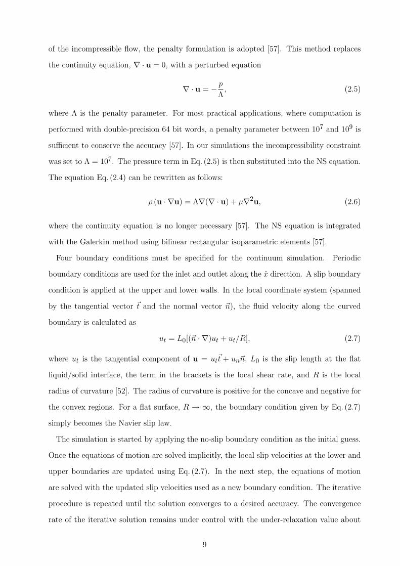
of the incompressible flow, the penalty formulation is adopted [57]. This method replaces

the continuity equation, ∇ · u = 0, with a perturbed equation

∇ · u = − p

Λ, (2.5)

where Λ is the penalty parameter. For most practical applications, where computation is

performed with double-precision 64 bit words, a penalty parameter between 107 and 109 is

sufficient to conserve the accuracy [57]. In our simulations the incompressibility constraint

was set to Λ = 107. The pressure term in Eq. (2.5) is then substituted into the NS equation.

The equation Eq. (2.4) can be rewritten as follows:

ρ (u · ∇u) = Λ∇(∇ · u) + µ∇2u, (2.6)

where the continuity equation is no longer necessary [57]. The NS equation is integrated

with the Galerkin method using bilinear rectangular isoparametric elements [57].

Four boundary conditions must be specified for the continuum simulation. Periodic

boundary conditions are used for the inlet and outlet along the x direction. A slip boundary

condition is applied at the upper and lower walls. In the local coordinate system (spanned

by the tangential vector ~t and the normal vector ~n), the fluid velocity along the curved

boundary is calculated as

ut = L0[(~n · ∇)ut + ut/R], (2.7)

where ut is the tangential component of u = ut~t + un~n, L0 is the slip length at the flat

liquid/solid interface, the term in the brackets is the local shear rate, and R is the local

radius of curvature [52]. The radius of curvature is positive for the concave and negative for

the convex regions. For a flat surface, R → ∞, the boundary condition given by Eq. (2.7)

simply becomes the Navier slip law.

The simulation is started by applying the no-slip boundary condition as the initial guess.

Once the equations of motion are solved implicitly, the local slip velocities at the lower and

upper boundaries are updated using Eq. (2.7). In the next step, the equations of motion

are solved with the updated slip velocities used as a new boundary condition. The iterative

procedure is repeated until the solution converges to a desired accuracy. The convergence

rate of the iterative solution remains under control with the under-relaxation value about

9

0.001 for the boundary nodes. In all continuum simulations, the grids at the lower boundary

have an aspect ratio of about one. The computational cost is reduced by increasing the

aspect ratio of the grids in the bulk region.

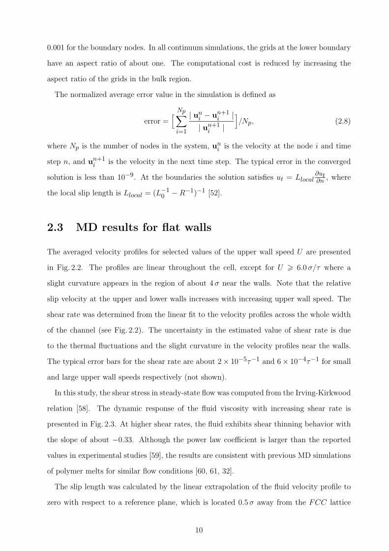
The normalized average error value in the simulation is defined as

error =[ Np∑

i=1

| uni − un+1

i || un+1

i |]/Np, (2.8)

where Np is the number of nodes in the system, uni is the velocity at the node i and time

step n, and un+1i is the velocity in the next time step. The typical error in the converged

solution is less than 10−9. At the boundaries the solution satisfies ut = Llocal∂ut∂n , where

the local slip length is Llocal = (L−10 −R−1)−1 [52].

2.3 MD results for flat walls

The averaged velocity profiles for selected values of the upper wall speed U are presented

in Fig. 2.2. The profiles are linear throughout the cell, except for U > 6.0 σ/τ where a

slight curvature appears in the region of about 4 σ near the walls. Note that the relative

slip velocity at the upper and lower walls increases with increasing upper wall speed. The

shear rate was determined from the linear fit to the velocity profiles across the whole width

of the channel (see Fig. 2.2). The uncertainty in the estimated value of shear rate is due

to the thermal fluctuations and the slight curvature in the velocity profiles near the walls.

The typical error bars for the shear rate are about 2× 10−5τ−1 and 6× 10−4τ−1 for small

and large upper wall speeds respectively (not shown).

In this study, the shear stress in steady-state flow was computed from the Irving-Kirkwood

relation [58]. The dynamic response of the fluid viscosity with increasing shear rate is

presented in Fig. 2.3. At higher shear rates, the fluid exhibits shear thinning behavior with

the slope of about −0.33. Although the power law coefficient is larger than the reported

values in experimental studies [59], the results are consistent with previous MD simulations

of polymer melts for similar flow conditions [60, 61, 32].

The slip length was calculated by the linear extrapolation of the fluid velocity profile to

zero with respect to a reference plane, which is located 0.5 σ away from the FCC lattice

10

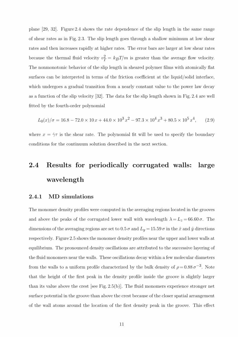
plane [29, 32]. Figure 2.4 shows the rate dependence of the slip length in the same range

of shear rates as in Fig. 2.3. The slip length goes through a shallow minimum at low shear

rates and then increases rapidly at higher rates. The error bars are larger at low shear rates

because the thermal fluid velocity v2T = kBT/m is greater than the average flow velocity.

The nonmonotonic behavior of the slip length in sheared polymer films with atomically flat

surfaces can be interpreted in terms of the friction coefficient at the liquid/solid interface,

which undergoes a gradual transition from a nearly constant value to the power law decay

as a function of the slip velocity [32]. The data for the slip length shown in Fig. 2.4 are well

fitted by the fourth-order polynomial

L0(x)/σ = 16.8− 72.0× 10 x + 44.0× 103 x2 − 97.3× 104 x3 + 80.5× 105 x4, (2.9)

where x = γτ is the shear rate. The polynomial fit will be used to specify the boundary

conditions for the continuum solution described in the next section.

2.4 Results for periodically corrugated walls: large

wavelength

2.4.1 MD simulations

The monomer density profiles were computed in the averaging regions located in the grooves

and above the peaks of the corrugated lower wall with wavelength λ = Lz = 66.60 σ. The

dimensions of the averaging regions are set to 0.5 σ and Ly = 15.59 σ in the x and y directions

respectively. Figure 2.5 shows the monomer density profiles near the upper and lower walls at

equilibrium. The pronounced density oscillations are attributed to the successive layering of

the fluid monomers near the walls. These oscillations decay within a few molecular diameters

from the walls to a uniform profile characterized by the bulk density of ρ = 0.88 σ−3. Note

that the height of the first peak in the density profile inside the groove is slightly larger

than its value above the crest [see Fig. 2.5(b)]. The fluid monomers experience stronger net

surface potential in the groove than above the crest because of the closer spatial arrangement

of the wall atoms around the location of the first density peak in the groove. This effect

11

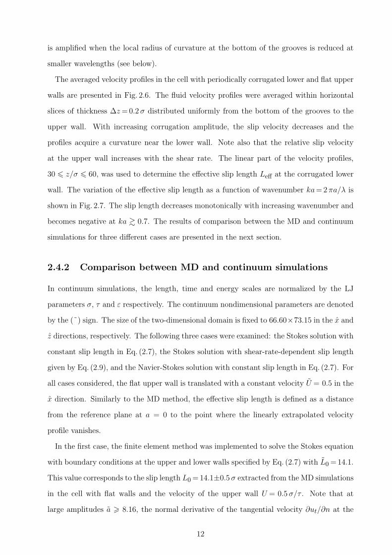
is amplified when the local radius of curvature at the bottom of the grooves is reduced at

smaller wavelengths (see below).

The averaged velocity profiles in the cell with periodically corrugated lower and flat upper

walls are presented in Fig. 2.6. The fluid velocity profiles were averaged within horizontal

slices of thickness ∆z = 0.2 σ distributed uniformly from the bottom of the grooves to the

upper wall. With increasing corrugation amplitude, the slip velocity decreases and the

profiles acquire a curvature near the lower wall. Note also that the relative slip velocity

at the upper wall increases with the shear rate. The linear part of the velocity profiles,

30 6 z/σ 6 60, was used to determine the effective slip length Leff at the corrugated lower

wall. The variation of the effective slip length as a function of wavenumber ka = 2 πa/λ is

shown in Fig. 2.7. The slip length decreases monotonically with increasing wavenumber and

becomes negative at ka & 0.7. The results of comparison between the MD and continuum

simulations for three different cases are presented in the next section.

2.4.2 Comparison between MD and continuum simulations

In continuum simulations, the length, time and energy scales are normalized by the LJ

parameters σ, τ and ε respectively. The continuum nondimensional parameters are denoted

by the (˜) sign. The size of the two-dimensional domain is fixed to 66.60×73.15 in the x and

z directions, respectively. The following three cases were examined: the Stokes solution with

constant slip length in Eq. (2.7), the Stokes solution with shear-rate-dependent slip length

given by Eq. (2.9), and the Navier-Stokes solution with constant slip length in Eq. (2.7). For

all cases considered, the flat upper wall is translated with a constant velocity U = 0.5 in the

x direction. Similarly to the MD method, the effective slip length is defined as a distance

from the reference plane at a = 0 to the point where the linearly extrapolated velocity

profile vanishes.

In the first case, the finite element method was implemented to solve the Stokes equation

with boundary conditions at the upper and lower walls specified by Eq. (2.7) with L0 = 14.1.

This value corresponds to the slip length L0 = 14.1±0.5 σ extracted from the MD simulations

in the cell with flat walls and the velocity of the upper wall U = 0.5 σ/τ . Note that at

large amplitudes a > 8.16, the normal derivative of the tangential velocity ∂ut/∂n at the

12

bottom of the grooves is negative, while the x component of the slip velocity is positive

everywhere along the corrugated lower wall. The dependence of the effective slip length on

the corrugation amplitude is shown in Fig. 2.7. The continuum results agree well with the

approximate analytical solution [52] for ka . 0.5 (not shown). For larger amplitudes, ka >

0.5, where the analytical solution is not valid, our results were tested to be grid independent.

There is an excellent agreement between slip lengths obtained from the MD and continuum

simulations for ka . 0.3. With further increasing the amplitude, the slip length obtained

from the continuum solution overestimates its MD value. The results presented in Fig. 2.7

are consistent with the analysis performed earlier for simple fluids [35], although a better

agreement between MD and continuum solutions was expected at ka > 0.5 because of the

larger system size considered in the present study.

As discussed in the previous section, the slip length for atomically flat walls is rate-

dependent even at low shear rates (see Fig. 2.4). In the second case, we include the effect

of shear rate in the analysis of the effective slip length at the corrugated lower wall and

flat upper wall. The Stokes equation is solved with boundary conditions given by Eq. (2.7),

where the slip length Eq. (2.9) is a function of the local shear rate at the curved and flat

boundaries. The results obtained from the Stokes solution with constant and rate-dependent

slip lengths are almost indistinguishable (see Fig. 2.7). This behavior can be attributed to

a small variation of the intrinsic slip length Eq. (2.9) at low shear rates. For example, at

the largest amplitude, a = 12.04, the local shear rate at the corrugated wall is position-

dependent and bounded by |∂ut/∂n + ut/R| 6 0.0035. In this range of shear rates, the

normalized value of the slip length in Eq. (2.9) varies between 14.7 6 L0 6 16.6. It is

expected, however, that the effect of shear rate will be noticeable at larger values of the top

wall speed U .

In the third case, the Navier-Stokes equation is solved with a constant slip length L0 = 14.1

in Eq. (2.7) at the flat upper and corrugated lower walls. The upper estimate of the Reynolds

number based on the fluid density ρ = 0.88, viscosity µ = 20.0, and the fluid velocity differ-

ence across the channel is Re≈ 1.3. It was previously shown by Tuck and Kouzoubov [63]

that at small ka and L0 = 0 the magnitude of the apparent slip velocity at the mean surface

increases due to finite Reynolds number effects for Re & 30. In our study, the difference

13

between the slip lengths extracted from the Stokes and Navier-Stokes solutions is within

the error bars (see Fig. 2.7). These results confirm that the slip length is not affected by the

inertia term in the Navier-Stokes equation for Re . 1.3. To check how sensitive the bound-

ary conditions are to higher Reynolds number flows, we have also repeated the continuum

simulations for larger velocity of the upper wall U = 50, which corresponds to Re≈ 130. For

the largest corrugation amplitude a = 12.04, the backflow appears inside the groove and the

effective slip length becomes smaller than its value for U = 0.5 by about 0.7 (not shown).

2.5 Results for periodically corrugated walls: small

wavelengths

2.5.1 Comparison between MD and continuum simulations

The MD simulations described in this section were performed at corrugation wavelengths

(λ/σ = 3.75, 7.5 and 22.5) comparable with the size of a polymer coil. Periodic surface rough-

ness of the lower wall was created by displacing the FCC wall atoms by ∆z = a sin(2 πx/λ)

in the z direction [35]. In order to reduce the computational time the system size was

restricted to Nf = 8580 fluid monomers and Lx = 22.5 σ, Ly = 12.5 σ and Lz = 35.6 σ. All

other system parameters were kept the same as in the previous section.

The representative density profiles near the upper and lower walls are shown in Fig. 2.8 for

the wavelength λ = 7.5 σ. The height of the first peak in the density profile is larger in the

grooves than near the flat wall or above the crests of the corrugated surface. The effective slip

length as a function of wavenumber ka is plotted in Fig. 2.9. For all wavelengths, the slip

length decreases monotonically with increasing values of ka. At the smallest wavelength

λ = 3.75 σ, the slip length rapidly decays to zero at ka≈ 0.4 and weakly depends on the

corrugation amplitude at larger ka. Inspection of the local velocity profiles for λ = 3.75 σ

and ka & 1.0 indicates that the flow is stagnant inside the grooves [62].

In the continuum analysis, the Stokes equation with a constant slip length L0 = 14.1 in

Eq. (2.7) is solved for the three wavelengths. The comparison between the MD results and

the solution of the Stokes equation is presented in Fig. 2.9. The error bars are larger for the

14

smallest wavelength because of the fine grid resolution required near the lower boundary at

ka . 0.2 (see inset in Fig. 2.9). The results shown in Fig. 2.9 confirm previous findings for

simple fluids [35] that the slip length obtained from the Stokes flow solution overestimates

its MD value and the agreement between the two solutions becomes worse at smaller wave-

lengths. It is interesting to note that the curves for different wavelengths intersect each

other at ka≈ 0.63 in the MD model and at ka≈ 1.02 in the continuum analysis. The same

trend was also observed in the previous study on slip flow of simple fluids past periodically

corrugated surfaces [35].

2.5.2 The polymer chain configuration and dynamics near rough

surfaces

In this section, the properties of polymer chains are examined in the bulk and near the

corrugated boundary with wavelengths λ = 3.5 σ and λ = 7.5 σ. The radius of gyration Rg

was computed as

R2g =

1

N

N∑

i=1(Ri −Rcm)2, (2.10)

where Ri is the three-dimensional position vector of a monomer, N = 20 is the number of

monomers in the chain, and Rcm is center of mass vector defined as

Rcm =1

N

N∑

i=1Ri. (2.11)

The chain statistics were collected in four different regions at equilibrium (U = 0) and

in the shear flow induced by the upper wall moving with velocity U = 0.5 σ/τ in the x

direction. Averaging regions were located above the peaks, in the grooves, near the flat

upper wall and in the bulk (see Fig. 2.10 for an example). The dimensions of the averaging

regions above the peaks and in the grooves of the lower wall are σ× 12.5 σ× 1.5 σ, and near

the upper wall and in the bulk are 22.5 σ × 12.5 σ × 1.5 σ. Three components of the radius

of gyration were computed for polymer chains with the center of mass inside the averaging

regions.

In the bulk region, the components of the radius of gyration remain the same for both

wavelengths, indicating that the chain orientation is isotropic at equilibrium and is not

15

affected by the confining walls. In the steady-state flow, the effective slip length is sup-

pressed by the surface roughness and, therefore, the shear rate in the bulk increases with

the corrugation amplitude. This explains why the x component of the radius of gyration

Rgx increases slightly at larger amplitudes (see Tables 2.1 and 2.2). Near the upper wall,

the polymer chains become flattened parallel to the surface and slightly stretched in the

presence of shear flow. These results are consistent with the previous MD simulations of

polymer melts confined between atomically flat walls [65, 30, 64].

In the case of a rough surface with the wavelength λ = 7.5 σ, a polymer chain can be

accommodated inside a groove (see Fig. 2.10 for an example). With increasing corrugation

amplitude, the polymer chains inside the grooves elongate along the y direction and contract

in the x direction (see Table 2.1). The tendency of the trapped molecules to orient parallel to

the grooves was observed previously in MD simulations of hexadecane [34]. In the presence

of shear flow, polymer chains are highly stretched in the x direction above the crests of the

wavy wall. A snapshot of the unfolded chains during migration between neighboring valleys

is shown in Fig. 2.10. The flow conditions in Fig. 2.10 correspond to a negative effective slip

length Leff ≈ −2 σ.

For the smallest corrugation wavelength λ = 3.75 σ, polymer chains cannot easily fit in

the grooves unless highly stretched. Therefore, the y component of the radius of gyration

is relatively large when the center of mass is located in the deep grooves (see Table 2.2).

Figure 2.11 shows a snapshot of several polymer chains in contact with the lower corrugated

wall. The chain segments are oriented parallel to the grooves and stretched above the crests

of the surface corrugation. Visual inspection of the consecutive snapshots reveals that the

chains near the corrugated wall move, on average, in the direction of shear flow; however,

their tails can be trapped for a long time because of the strong net surface potential inside

the grooves. For large wavenumbers ka & 0.5, the magnitude of the negative effective

slip length is approximately equal to the sum of the corrugation amplitude and Rgz of the

polymer chains above the crests of the wavy wall.

16

2.6 Conclusions

In this chapter the effects of the shear rate and surface roughness on slip flow of a poly-

mer melt was studied using molecular dynamics and continuum simulations. The linear

part of the velocity profiles in the steady-state flow was used to calculate the effective slip

length and shear rate. For atomically flat walls, the slip length passes through a shallow

minimum at low shear rates and then increases rapidly at higher shear rates. In the case

of periodic surface heterogeneities with the wavelength larger than the radius of gyration,

the effective slip length decays monotonically with increasing the corrugation amplitude.

For small wavenumbers, the effective slip length obtained from the solution of the Stokes

equation with constant and shear-dependent local slip length is in a good agreement with

its values computed from the MD simulations, in accordance with the previous analysis for

simple fluids [35]. At low Reynolds numbers, the inertial effects on slip boundary conditions

are negligible. When the corrugation wavelengths are comparable to the radius of gyration,

polymer chains stretch in the direction of shear flow above the crests of the surface corru-

gation, while the chains located in the grooves elongate perpendicular to the flow. In this

regime the continuum approach fails to describe accurately the rapid decay of the effective

slip length with increasing wavenumber.

17

a

L

λ

U

ux(z)

xzy

Solid Wall

Leff

z

Figure 2.1. For interpretation of the references to color in this and all other figures, the

reader is referred to the electronic version of this dissertation. A snapshot of the fluid

monomers (open circles) confined between solid walls (closed circles) obtained from the MD

simulations. The atoms of the stationary lower wall are distributed along the sinusoidal

curve with the wavelength λ and amplitude a. The flat upper wall is moving with a constant

velocity U in the x direction. The effective slip length Leff is determined by the linear

extrapolation of the velocity profile to ux = 0.

18

10 20 30 40 50 60 700

1

2

3

4

5

6

7

8

σz

< u

x> τ

/ σ

/

U = 1.0 σ/τ U = 2.0 σ/τ U = 4.0 σ/τ U = 6.0 σ/τ U = 8.0 σ/τ

Figure 2.2. Averaged velocity profiles in the cell with flat upper and lower walls. The solid

lines are the best linear fit to the data. The vertical axes indicate the location of the FCC

lattice planes. The velocities of the upper wall are tabulated in the inset.

19

-3.5 -3.0 -2.5 -2.0 -1.5 -1.00.8

0.9

1.0

1.1

1.2

1.3

1.4

lo

g 10 ( µ

/ε τ σ

−3 )

-0.33

Lx = 66.60 σLz = 74.15 σ

ρw = 1.94 σ -3

εwf = 1.0 εσwf = 1.0 σ

log10(γτ).

Figure 2.3. Viscosity of the polymer melt µ/ετσ−3 as a function of shear rate. The dashed

line with the slope −0.33 is plotted for reference.

20

-3.5 -3.0 -2.5 -2.0 -1.5 -1.00

5

10

15

20

25

30

Ls /σ

log10(γτ)

ρw = 1.94 σ -3

εwf = 1.0 εσwf = 1.0 σ

Lx = 66.60 σLz = 74.15 σ

.

Figure 2.4. Variation of the slip length as a function of shear rate in the cell with flat upper

and lower walls. The solid line is a fourth-order polynomial fit to the data given by Eq. (2.9).

21

68 70 72 74

-6 -4 10 120

2

4

0

2

4 Inside the groove Above the peak

ρ σ 3

(b)

σz /

0

2

4

0

2

4

Flat upper wall

(a)

Figure 2.5. Averaged density profiles near the stationary upper wall (a), above the peak

and in the groove of the lower wall with amplitude a = 8.16 σ and wavelength λ = 66.60 σ

(b).

22

-10 0 10 20 30 40 50 60 700.0

0.1

0.2

0.3

0.4

0.5

Flat walls a = 3.52 σ a = 7.24 σ a = 12.04 σ

< u

x> τ

/ σ

σz /

U = 0.5 σ /τ

Lz = 74.15 σ λ = 66.60 σ

Figure 2.6. Averaged velocity profiles for the indicated values of the corrugation amplitude

a. The vertical dashed line denotes a reference plane for calculation of the effective slip

length at the corrugated lower wall. The velocity of the flat upper wall is U = 0.5 σ/τ .

23

0.0 0.2 0.4 0.6 0.8 1.0 1.2

-4

0

4

8

12

16

Stokes L0( γ τ )

Navier-Stokes

.

MD simulation Stokes L0= constant

ka

Lef

f /σ

U = 0.5 σ /τ

Lz = 74.15 σ λ = 66.60 σ

Figure 2.7. The effective slip length as a function of wavenumber ka obtained from the MD

simulations (¨), the solution of the Stokes equation with rate-independent slip length L0() and with L0(γτ) given by Eq. (2.9) (×), the solution of the Navier-Stokes equation with

L0 (M).

24

28 30 32 34 36

0

2

4

0

2

4

6

0 2 4 6 80

2

4

6ρ σ 3

Inside the groove Above the peak

(b)

σz /

0

2

4

(a) Flat upper wall

Figure 2.8. Averaged fluid density profiles near flat upper wall (a) and corrugated lower

wall with amplitude a = 1.4 σ and wavelength λ = 7.5 σ (b). The velocity of the upper wall

is U = 0.5 σ/τ .

25

0.0 0.4 0.8 1.2 1.6-8

-4

0

4

8

12

Lef

f /σ

ka L

eff /σ

λ = 3.75 σ λ = 7.5 σ λ = 22.5 σ

ka

0.0 0.1 0.24

8

12

Figure 2.9. The effective slip length as a function of wavenumber ka for the indicated values

of wavelength λ. Continuum results are denoted by the dashed lines and open symbols,

while the MD results are shown by straight lines and filled symbols. The inset shows the

same data for ka 6 0.25.

26

λ = 7.5 σ a = 0.2 σ a = 0.6 σ a = 1.4 σ

Rgx Rgy Rgz Rgx Rgy Rgz Rgx Rgy Rgz

Bulk Equilibrium 1.18 1.18 1.18 1.18 1.18 1.18 1.18 1.18 1.18

Shear flow 1.70 1.11 1.04 1.76 1.10 1.02 1.79 1.10 1.01

Upper Equilibrium 1.34 1.37 0.66 1.35 1.36 0.66 1.35 1.35 0.66

wall Shear flow 1.63 1.29 0.63 1.64 1.29 0.63 1.67 1.29 0.63

Peak Equilibrium 1.35 1.36 0.69 1.40 1.31 0.76 1.46 1.27 0.84

Shear flow 1.65 1.28 0.67 1.85 1.21 0.75 2.17 1.10 0.93

Groove Equilibrium 1.31 1.37 0.63 1.10 1.47 0.61 0.77 1.69 0.61

Shear flow 1.50 1.34 0.62 1.19 1.44 0.60 0.75 1.89 0.59

Table 2.1. Averaged x, y, and z components of the radius of gyration at equilibrium and in the shear flow. The Rg values are reported in

the bulk, near the flat upper wall, above the peaks, and inside the grooves. The wavelength of the lower wall is λ = 7.5 σ. The size of the

averaging region inside the grooves and above the peaks is σ × 12.5 σ × 1.5 σ. The estimate of the error bars is ±0.03 σ.

27

λ = 3.75 σ a = 0.07 σ a = 0.2 σ a = 1.0 σ

Rgx Rgy Rgz Rgx Rgy Rgz Rgx Rgy Rgz

Bulk Equilibrium 1.18 1.18 1.18 1.18 1.18 1.18 1.18 1.18 1.18

Shear flow 1.70 1.12 1.03 1.76 1.10 1.02 1.78 1.10 1.01

Upper Equilibrium 1.33 1.36 0.66 1.36 1.34 0.66 1.37 1.34 0.65

wall Shear flow 1.60 1.32 0.63 1.64 1.29 0.63 1.65 1.27 0.63

Peak Equilibrium 1.38 1.33 0.67 1.42 1.30 0.71 1.41 1.25 0.92

Shear flow 1.61 1.27 0.65 1.66 1.26 0.69 1.78 1.17 0.84

Groove Equilibrium 1.33 1.36 0.64 1.25 1.42 0.61 0.48 2.64 0.55

Shear flow 1.60 1.29 0.61 1.60 1.33 0.59 0.47 2.70 0.54

Table 2.2. Averaged x, y, and z components of the radius of gyration at equilibrium and in the shear flow. The Rg values are reported in

the bulk, near the flat upper wall, above the peaks, and inside the grooves. The wavelength of the lower wall is λ = 3.75 σ. The dimensions

of the averaging region are the same as in Table 2.1.

28

x

yz

σ

σσ 1.512.5

Figure 2.10. A snapshot of four polymer chains near the lower corrugated wall for wavelength

λ = 7.5 σ and amplitude a = 1.4 σ. The velocity of the upper wall is U = 0.5 σ/τ .

29

xy

xz

σ

σ

σ1.5

σ12.5

Figure 2.11. A snapshot of five polymer chains near the lower corrugated wall for the

wavelength λ = 3.75 σ and amplitude a = 1.0 σ. The figure shows the side view (top) and

the top view (bottom). The velocity of the upper wall is U = 0.5 σ/τ .

30

CHAPTER 3

Slip boundary conditions for shear

flow of polymer melts past atomically

flat surfaces

3.1 Introduction

The fluid flow in microfluidic channels can be significantly influenced by liquid slip at the

solid boundary because of the large surface to volume ratio [67]. The Navier model for

the partial slip boundary conditions relates the fluid slip velocity to the tangential viscous

stress at the wall via the friction coefficient, which is defined as the ratio of the shear

viscosity to the slip length. Geometrically, the slip length is determined as a distance from

the solid wall where the linearly extrapolated fluid velocity profile vanishes. Experimental

studies have demonstrated that for atomically smooth surfaces the slip length is relatively

large for non-wetting liquid/solid interfaces [5, 15, 117], polymeric fluids [68, 16] and high

shear rates [69, 17, 19]. By contrast, surface roughness even on the submicron length scale

strongly reduces the degree of slip for both polymeric [12] and Newtonian [10, 14, 13] fluids.

However, experimentally it is often difficult to isolate and, consequently, to analyze the

effects of wettability, surface roughness and shear rate on slip boundary conditions because

of the small scales involved.

During the past two decades, a number of molecular dynamics (MD) simulations [20,

31

21, 121, 25, 24, 26, 27, 28, 40, 29] have been performed to investigate the dependence of

the slip length on the structure of dense fluids near atomically flat surfaces. For simple

fluids, it has been well established that the slip length correlates inversely with the wall-

fluid interaction energy and the surface induced order in the first fluid layer [21, 121, 29].

The strong wall-fluid coupling and commensurate structures of the liquid/solid interface

lead to the no-slip boundary condition for monoatomic fluids [21, 28]. The interfacial slip

is enhanced in the flow of polymer melts due to the higher shear viscosity and reduced

molecular ordering near the flat wall [125, 30, 31, 27]. The magnitude of the slip length in

the flow of polycarbonate blends past atomically smooth nickel surfaces is determined by the

competition between the apparent slip of the adsorbed polymer layer and its thickness [70].

The slip boundary conditions for the polymer melt flow over the brush can be controlled

by changing the density of the end-grafted polymer layer [71]. Finally, the degree of slip at

the interface between immiscible polymers is larger for longer chain molecules and greater

repulsion between unlike species [72].

Until ten years ago, the slip length in the Navier model was assumed to be independent of

shear rate. In the seminal MD study by Thompson and Troian [23] on shear flow of simple

fluids past atomically flat rigid walls, it was found that the slip length increases nonlinearly

with the shear rate. Upon increasing the surface energy, a gradual transition from the power

law behavior [23] to the linear rate dependence was recently reported for weak wall-fluid

interactions and incommensurate structures of the liquid/solid interface [29]. In a wide

range of shear rates and surface energies, the slip length in simple fluids is determined by a

function of the in-plane structure factor, contact density and temperature of the first fluid

layer near the wall [29]. The rate-dependent slip length at the interface between a polymer

melt composed of short linear chains and a crystalline substrate is also well described by the

power law function used to fit the data for simple fluids [27, 23]. Whether these boundary

conditions hold for higher molecular weight polymers or rough surfaces is an open question

that has to be addressed for the correct interpretation of the experimental results and

modeling fluid flows in microfluidic channels.

In this chapter, the effects of shear rate and fluid density on slip boundary conditions for

the flow of a polymer melt past a crystalline wall are investigated by molecular dynamics

32

simulations. We will show that the rate-dependent slip length reaches a local minimum

and then increases rapidly at higher shear rates. In the shear thinning regime, the friction

coefficient at the liquid/solid interface follows a power law decay as a function of the slip

velocity. In a wide range of shear rates and polymer densities, the ratio of the slip length

to the shear viscosity is determined by the surface induced structure in the first fluid layer.

These results suggest that the correlation between the fluid structure near the flat wall and

the slip length is determined by a universal combination of parameters for both polymer

melts and simple fluids [29].

This chapter is organized as follows. The molecular dynamics simulation model and

parameter values are described in the next section. The results for the rate dependence of

the slip length and the analysis of the fluid structure near the solid wall are presented in

Section 5.3. The conclusions are given in the last section.

3.2 Details of molecular dynamics simulations

The polymer melt is confined between two atomically flat walls and is subject to planar

shear in the x direction (see Fig. 3.1 for a schematic representation). The fluid monomers

interact through the pairwise Lennard-Jones (LJ) potential

VLJ (r)= 4 ε[(σ

r

)12−(σ

r

)6 ], (3.1)

with a cutoff distance rc = 2.5 σ, where ε and σ represent the energy and length scales of

the fluid phase. The total number of monomers is Nf = 6000. The wall-fluid interaction

parameters of the LJ potential are set to εwf = 0.9 ε and σwf = σ throughout the study.

The polymer melt is modeled as a collection of bead-spring chains of N = 20 LJ monomers

interacting through the FENE (finitely extensible nonlinear elastic) potential [59]

VFENE(r) = −k

2r2o ln[1− r2/r2

o ], (3.2)

with Kremer and Grest parameters k = 30 εσ−2 and ro = 1.5 σ [53]. This choice of parameters

prevents polymer chains from unphysical crossing or bond breaking [54].

The system was coupled to an external heat bath through a Langevin thermostat [54]

with a random force and a damping term with a small value of the friction coefficient

33

Γ = 1.0 τ−1 [73]. The thermostat was only applied to the equation of motion for a fluid

monomer along the y axis to avoid a bias in the shear flow direction [21]. The equations of

motion for the x, y and z components are given by

mxi = −∑

i6=j

∂Vij

∂xi, (3.3)

myi + mΓyi = −∑

i6=j

∂Vij

∂yi+ fi , (3.4)

mzi = −∑

i6=j

∂Vij

∂zi, (3.5)

where fi is a random force with zero mean and variance 〈fi(0)fj(t)〉= 2mkBTΓδ(t)δij , the

temperature is T = 1.1 ε/kB and kB is the Boltzmann constant. The equations of motion

for fluid monomers and wall atoms were integrated using the fifth-order gear-predictor al-

gorithm [56] with a time step 4t = 0.002 τ , where τ =√

mσ2/ε is the characteristic time of

the LJ potential.

Each wall was constructed out of 576 LJ atoms, which formed two (111) layers of the

face-centered cubic (FCC) lattice with the density ρw = 1.40 σ−3. The corresponding

nearest-neighbor distance between equilibrium positions of the wall atoms in the xy plane is

d = 1.0 σ. The dimensions of the Couette cell (xyz) were held fixed to 20.86 σ× 12.04 σ×h,

where h is the channel height (see Table 3.1). The MD simulations were performed at a

constant density ensemble. The fluid density is defined as a ratio of the total number of

monomers to the volume accessible to the fluid, i.e., 0.5 σw away from the FCC lattice planes

in the z direction. The range of fluid densities considered in this study is 0.86 6 ρ σ3 6 1.02.

The pressures of the system at equilibrium are given in Table 3.1 for each value of the fluid

density. Periodic boundary conditions were employed along the x and y directions parallel

to the confining walls.

ρ [ σ−3] 0.86 0.88 0.91 0.94 1.00 1.02

P [ ε σ−3] 0.0 0.5 1.0 2.0 4.0 5.0

h [σ] 28.93 28.18 27.27 26.32 24.85 24.36

Table 3.1. The fluid pressure P at equilibrium, i.e., with the stationary upper wall, and the

channel height h (defined as a distance between the inner FCC planes) as a function of the

fluid density.

34

The wall atoms were attached to their equilibrium FCC lattice positions by the harmonic

spring with the potential Vsp = 12 κ r2. The spring stiffness κ = 1200 ε/σ2 is large enough so

that the mean-square displacement of the wall atoms is less than the Lindemann criterion

for melting, i.e., 〈δu2〉/d 2 . 0.023 (see Ref. [74]). In a recent paper on shear flow of

simple fluids [37], it was shown that the slope of the rate-dependent slip length remains

approximately the same for the thermal walls with κ = 1200 ε/σ2 and rigid FCC walls. The

friction term and the random force were also added to the x, y and z components of the

wall atoms equations of motion

mw xi + mw Γxi = −∑

i6=j

∂Vij

∂xi− ∂Vsp

∂xi+ fi , (3.6)

mw yi + mw Γyi = −∑

i6=j

∂Vij

∂yi− ∂Vsp

∂yi+ fi , (3.7)

mw zi + mw Γzi = −∑

i6=j

∂Vij

∂zi− ∂Vsp

∂zi+ fi , (3.8)

where the mass of the wall atoms is mw = 10 m and the summation is performed only over

the fluid monomers within the cutoff distance rc = 2.5 σ.

The simulations began with an equilibration period of about 5×104τ with both walls being

at rest. Then, the steady-state shear flow was generated by translating the upper wall with

a constant velocity U in the x direction, while the lower wall always remained stationary

(see Fig. 3.1). The fluid velocity profiles were computed by averaging the instantaneous

monomer velocities in the x direction within bins of thickness ∆z=0.2 σ for a time interval

up to 4×105τ at the lowest shear rates. The density profiles were averaged for a time period

5×104τ within bins of thickness of only ∆z = 0.01 σ to accurately resolve the fluid structure

near the walls [29]. The maximum value of the Reynolds number is Re≈ 10.5, which was

estimated from the maximum fluid velocity difference across the channel, the shear viscosity,

and the channel height. The small values of the Reynolds number correspond to laminar

flow conditions even at the highest shear rates considered in this study.

35

3.3 Results

3.3.1 Fluid density and velocity profiles

The fluid structure in the direction perpendicular to a flat surface usually consists of several

distinct layers on the molecular scale [75]. Examples of the averaged monomer density

profiles near the lower thermal wall are presented in Fig. 3.2 for three values of the upper

wall velocity. The highest peak is associated with a layer of fluid monomers (each connected

to a polymer chain) in contact with the wall atoms. The contact density ρc corresponds

to the maximum value of the peak. The density oscillations gradually decay away from

the wall to a uniform profile with bulk density ρ = 0.91 σ−3. The amplitude of the density

oscillations is reduced at higher values of the slip velocity.

Figure 3.3 shows the averaged velocity profiles for the same values of the upper wall speed

as in Fig. 3.2 and the fluid density ρ = 0.91 σ−3. For a given U , the relative slip velocity is

the same at the upper and lower walls. Surprisingly, the scaled slip velocity is smaller at

the intermediate speed of the upper wall U = 1.0 σ/τ . Because of the thermal fluctuations,

longer averaging times (up to 4×105τ) were required to accurately resolve the fluid velocity

profile for U = 0.05 σ/τ . A small curvature in the velocity profile is evident for the largest

velocity of the upper wall U = 5.0 σ/τ . The deviation from the linearity might be related to

the heating up of the fluid near the walls (see discussion below). The slope of the velocity

profile (used for calculation of the slip length and the shear rate) was computed from the

central part of the velocity profile excluding the data from the region of about 2 σ near the

walls.

We comment that at small shear rates, γτ . 0.01, and higher fluid densities, ρ & 1.04 σ−3,

the fluid velocity profiles acquired a pronounced curvature within a distance of about 4 σ

from the walls. The linearity of the fluid velocity profiles is restored at higher shear rates.

This effect will be examined in a separate study.

3.3.2 Rate dependence of the slip length and shear viscosity

In the MD study by Thompson and Troian [23] on shear flow of Newtonian liquids past

atomically flat surfaces, the slip length was found to increase nonlinearly with the shear

36

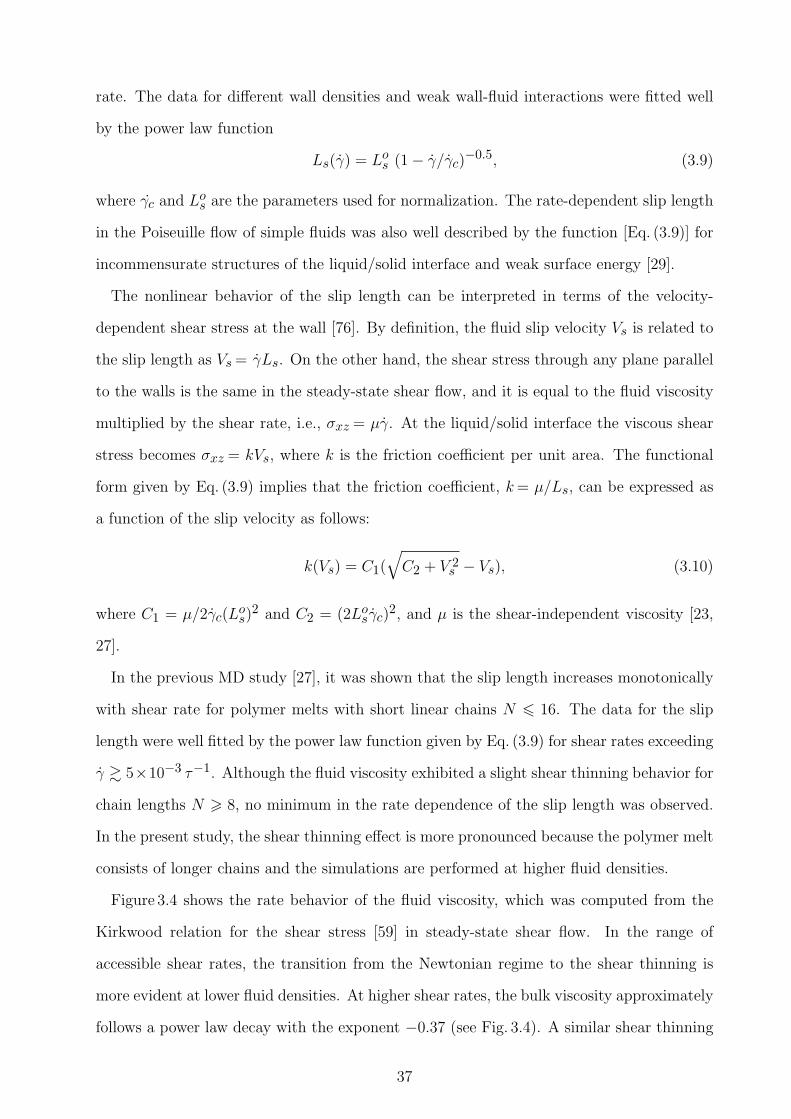
rate. The data for different wall densities and weak wall-fluid interactions were fitted well

by the power law function

Ls(γ) = Los (1− γ/γc)

−0.5, (3.9)

where γc and Los are the parameters used for normalization. The rate-dependent slip length

in the Poiseuille flow of simple fluids was also well described by the function [Eq. (3.9)] for

incommensurate structures of the liquid/solid interface and weak surface energy [29].

The nonlinear behavior of the slip length can be interpreted in terms of the velocity-

dependent shear stress at the wall [76]. By definition, the fluid slip velocity Vs is related to

the slip length as Vs = γLs. On the other hand, the shear stress through any plane parallel

to the walls is the same in the steady-state shear flow, and it is equal to the fluid viscosity

multiplied by the shear rate, i.e., σxz = µγ. At the liquid/solid interface the viscous shear

stress becomes σxz = kVs, where k is the friction coefficient per unit area. The functional

form given by Eq. (3.9) implies that the friction coefficient, k = µ/Ls, can be expressed as

a function of the slip velocity as follows:

k(Vs) = C1(√

C2 + V 2s − Vs), (3.10)

where C1 = µ/2γc(Los)

2 and C2 = (2Losγc)

2, and µ is the shear-independent viscosity [23,

27].

In the previous MD study [27], it was shown that the slip length increases monotonically

with shear rate for polymer melts with short linear chains N 6 16. The data for the slip

length were well fitted by the power law function given by Eq. (3.9) for shear rates exceeding

γ & 5×10−3 τ−1. Although the fluid viscosity exhibited a slight shear thinning behavior for

chain lengths N > 8, no minimum in the rate dependence of the slip length was observed.

In the present study, the shear thinning effect is more pronounced because the polymer melt

consists of longer chains and the simulations are performed at higher fluid densities.

Figure 3.4 shows the rate behavior of the fluid viscosity, which was computed from the

Kirkwood relation for the shear stress [59] in steady-state shear flow. In the range of

accessible shear rates, the transition from the Newtonian regime to the shear thinning is

more evident at lower fluid densities. At higher shear rates, the bulk viscosity approximately

follows a power law decay with the exponent −0.37 (see Fig. 3.4). A similar shear thinning

37

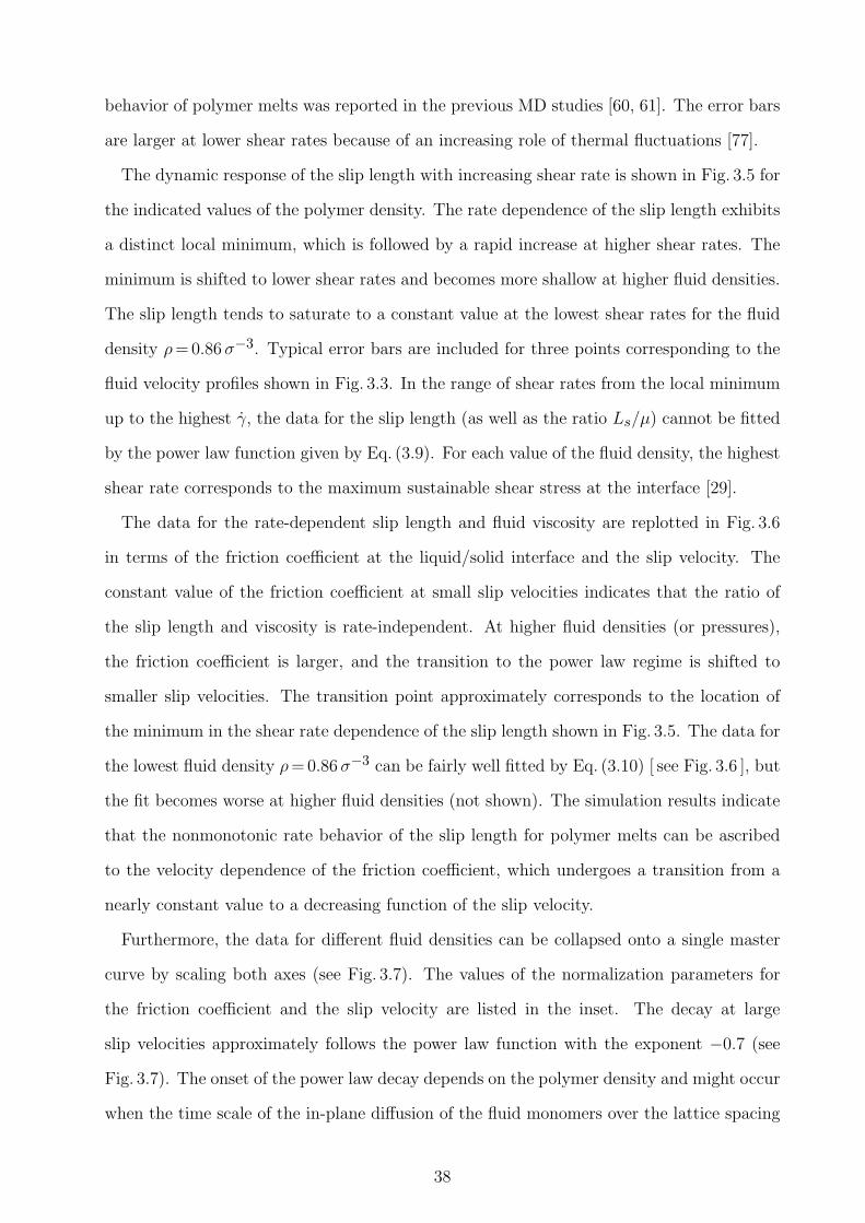
behavior of polymer melts was reported in the previous MD studies [60, 61]. The error bars

are larger at lower shear rates because of an increasing role of thermal fluctuations [77].

The dynamic response of the slip length with increasing shear rate is shown in Fig. 3.5 for

the indicated values of the polymer density. The rate dependence of the slip length exhibits

a distinct local minimum, which is followed by a rapid increase at higher shear rates. The

minimum is shifted to lower shear rates and becomes more shallow at higher fluid densities.

The slip length tends to saturate to a constant value at the lowest shear rates for the fluid

density ρ = 0.86 σ−3. Typical error bars are included for three points corresponding to the

fluid velocity profiles shown in Fig. 3.3. In the range of shear rates from the local minimum

up to the highest γ, the data for the slip length (as well as the ratio Ls/µ) cannot be fitted

by the power law function given by Eq. (3.9). For each value of the fluid density, the highest

shear rate corresponds to the maximum sustainable shear stress at the interface [29].

The data for the rate-dependent slip length and fluid viscosity are replotted in Fig. 3.6

in terms of the friction coefficient at the liquid/solid interface and the slip velocity. The

constant value of the friction coefficient at small slip velocities indicates that the ratio of

the slip length and viscosity is rate-independent. At higher fluid densities (or pressures),

the friction coefficient is larger, and the transition to the power law regime is shifted to

smaller slip velocities. The transition point approximately corresponds to the location of

the minimum in the shear rate dependence of the slip length shown in Fig. 3.5. The data for

the lowest fluid density ρ = 0.86 σ−3 can be fairly well fitted by Eq. (3.10) [ see Fig. 3.6 ], but

the fit becomes worse at higher fluid densities (not shown). The simulation results indicate

that the nonmonotonic rate behavior of the slip length for polymer melts can be ascribed

to the velocity dependence of the friction coefficient, which undergoes a transition from a

nearly constant value to a decreasing function of the slip velocity.

Furthermore, the data for different fluid densities can be collapsed onto a single master

curve by scaling both axes (see Fig. 3.7). The values of the normalization parameters for

the friction coefficient and the slip velocity are listed in the inset. The decay at large

slip velocities approximately follows the power law function with the exponent −0.7 (see

Fig. 3.7). The onset of the power law decay depends on the polymer density and might occur

when the time scale of the in-plane diffusion of the fluid monomers over the lattice spacing

38

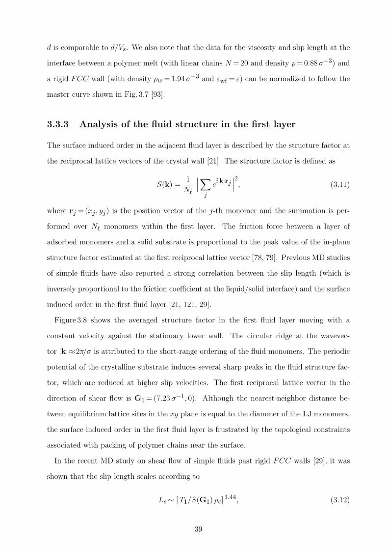
d is comparable to d/Vs. We also note that the data for the viscosity and slip length at the

interface between a polymer melt (with linear chains N = 20 and density ρ = 0.88 σ−3) and

a rigid FCC wall (with density ρw = 1.94 σ−3 and εwf = ε) can be normalized to follow the

master curve shown in Fig. 3.7 [93].

3.3.3 Analysis of the fluid structure in the first layer

The surface induced order in the adjacent fluid layer is described by the structure factor at

the reciprocal lattice vectors of the crystal wall [21]. The structure factor is defined as

S(k) =1

N`

∣∣∣∑

j

eik·rj

∣∣∣2, (3.11)

where rj = (xj , yj) is the position vector of the j-th monomer and the summation is per-

formed over N` monomers within the first layer. The friction force between a layer of

adsorbed monomers and a solid substrate is proportional to the peak value of the in-plane

structure factor estimated at the first reciprocal lattice vector [78, 79]. Previous MD studies

of simple fluids have also reported a strong correlation between the slip length (which is

inversely proportional to the friction coefficient at the liquid/solid interface) and the surface

induced order in the first fluid layer [21, 121, 29].

Figure 3.8 shows the averaged structure factor in the first fluid layer moving with a

constant velocity against the stationary lower wall. The circular ridge at the wavevec-

tor |k|≈2π/σ is attributed to the short-range ordering of the fluid monomers. The periodic

potential of the crystalline substrate induces several sharp peaks in the fluid structure fac-

tor, which are reduced at higher slip velocities. The first reciprocal lattice vector in the

direction of shear flow is G1 = (7.23 σ−1, 0). Although the nearest-neighbor distance be-

tween equilibrium lattice sites in the xy plane is equal to the diameter of the LJ monomers,

the surface induced order in the first fluid layer is frustrated by the topological constraints

associated with packing of polymer chains near the surface.

In the recent MD study on shear flow of simple fluids past rigid FCC walls [29], it was

shown that the slip length scales according to

Ls∼ [ T1/S(G1) ρc]1.44, (3.12)

39

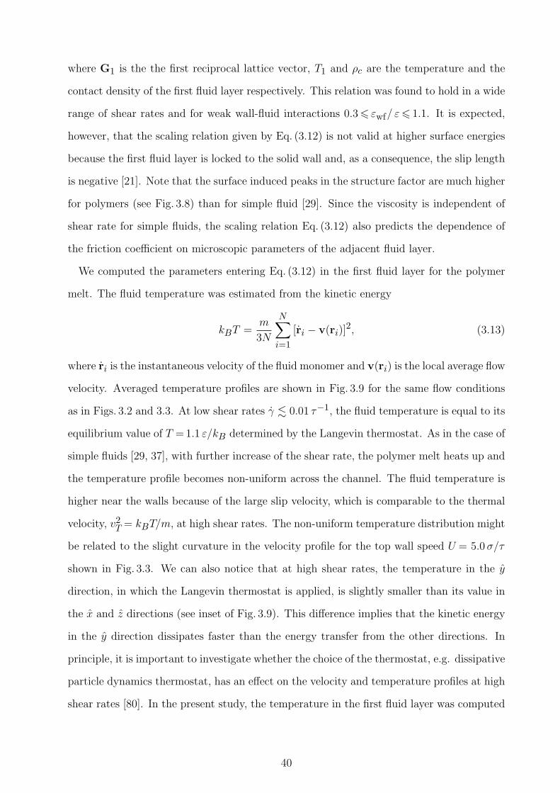
where G1 is the the first reciprocal lattice vector, T1 and ρc are the temperature and the

contact density of the first fluid layer respectively. This relation was found to hold in a wide

range of shear rates and for weak wall-fluid interactions 0.3 6 εwf/ ε 6 1.1. It is expected,

however, that the scaling relation given by Eq. (3.12) is not valid at higher surface energies

because the first fluid layer is locked to the solid wall and, as a consequence, the slip length

is negative [21]. Note that the surface induced peaks in the structure factor are much higher

for polymers (see Fig. 3.8) than for simple fluid [29]. Since the viscosity is independent of

shear rate for simple fluids, the scaling relation Eq. (3.12) also predicts the dependence of

the friction coefficient on microscopic parameters of the adjacent fluid layer.

We computed the parameters entering Eq. (3.12) in the first fluid layer for the polymer

melt. The fluid temperature was estimated from the kinetic energy

kBT =m

3N

N∑

i=1[ri − v(ri)]

2, (3.13)

where ri is the instantaneous velocity of the fluid monomer and v(ri) is the local average flow

velocity. Averaged temperature profiles are shown in Fig. 3.9 for the same flow conditions

as in Figs. 3.2 and 3.3. At low shear rates γ . 0.01 τ−1, the fluid temperature is equal to its

equilibrium value of T = 1.1 ε/kB determined by the Langevin thermostat. As in the case of

simple fluids [29, 37], with further increase of the shear rate, the polymer melt heats up and

the temperature profile becomes non-uniform across the channel. The fluid temperature is

higher near the walls because of the large slip velocity, which is comparable to the thermal

velocity, v2T = kBT/m, at high shear rates. The non-uniform temperature distribution might

be related to the slight curvature in the velocity profile for the top wall speed U = 5.0 σ/τ

shown in Fig. 3.3. We can also notice that at high shear rates, the temperature in the y

direction, in which the Langevin thermostat is applied, is slightly smaller than its value in

the x and z directions (see inset of Fig. 3.9). This difference implies that the kinetic energy

in the y direction dissipates faster than the energy transfer from the other directions. In

principle, it is important to investigate whether the choice of the thermostat, e.g. dissipative

particle dynamics thermostat, has an effect on the velocity and temperature profiles at high

shear rates [80]. In the present study, the temperature in the first fluid layer was computed

40

from

T1 =

∫ z1

z0T (z)ρ(z)dz

/ ∫ z1

z0ρ(z)dz, (3.14)

where the limits of integration (z0 = −14.4 σ and z1 = −13.8 σ) are given by the width of

the first peak in the density profile (e.g. see Fig. 3.2).

The ratio of the slip length to viscosity is plotted in Fig. 3.10 as a function of T1/[S(G1) ρc]

for different fluid densities and shear rates. Except for higher densities at low shear rates, the

data collapse onto a single curve, which approximately follows the power law function with

a slope of 0.9 (see Fig. 3.10). Although the slope is different from the value 1.44 reported for

simple fluids [29], it is remarkable that the same combination of parameters determines the

boundary conditions for both polymer melts and simple fluids. The simulation results also

show that for each value of the fluid density, the number of fluid monomers in the first layer

N` = S(0) decreases by about 4% at the highest shear rates. The same data for the slip

length and viscosity are replotted as a function of the variable S(0)/ [S(G1) ρc] in Fig. 3.11.

The collapse of the data is consistent with the previous results for the rate-independent

slip length at the interface between simple fluids and crystalline walls [21]. The correlation

between the friction coefficient and the fluid structure in the adjacent layer presented in

Figs. 3.10 and 3.11 suggests a possible existence of a general functional relation between the

slip length, shear rate and polymer density.

3.4 Conclusions

In this chapter, the rate dependence of the slip length in the shear flow of polymer melts

past atomically smooth, thermal surfaces was studied using molecular dynamics simulations.

For weak wall-fluid interactions, the slip length passes through a minimum as a function of

shear rate and then increases rapidly at higher shear rates. The nonlinear rate dependence

of the slip length was analyzed in terms of the dynamic friction at the liquid/solid interface.

In a wide range of fluid densities, the friction coefficient (the ratio of the shear viscosity

and the slip length) undergoes a universal transition from a constant value to the power law

decay as a function of the slip velocity. The simulation results for polymer melts confirm the

previous findings for simple fluids [29] that the surface induced structure and the contact

41

density of the adjacent fluid layer are crucial factors for determining the value of the friction

coefficient.

42

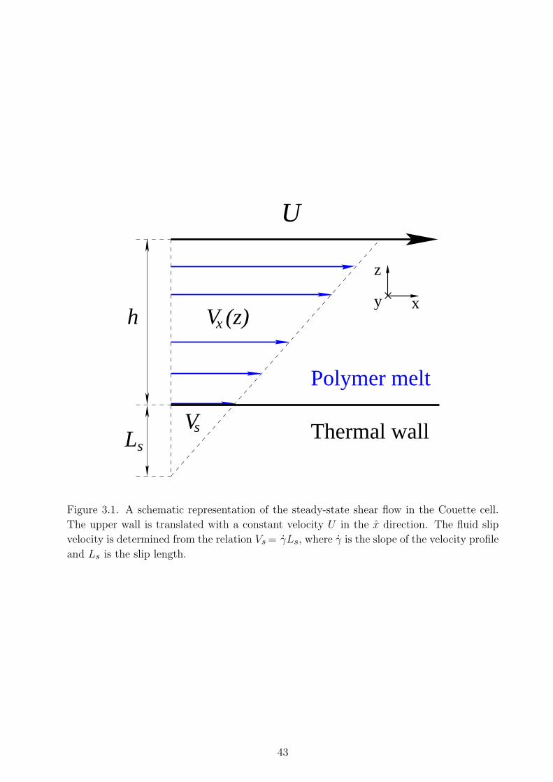
V (z)x

Vs

x

z

U

Ls

Polymer melt

Thermal wall

yh

Figure 3.1. A schematic representation of the steady-state shear flow in the Couette cell.

The upper wall is translated with a constant velocity U in the x direction. The fluid slip

velocity is determined from the relation Vs = γLs, where γ is the slope of the velocity profile

and Ls is the slip length.

43

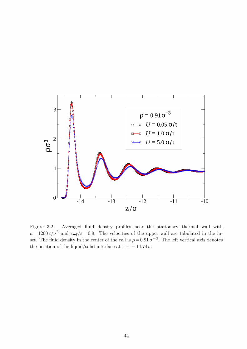
-14 -13 -12 -11 -10z/σ

0

1

2

3

ρσ3

ρ = 0.91σ−3

U = 0.05 σ/τU = 1.0 σ/τU = 5.0 σ/τ

Figure 3.2. Averaged fluid density profiles near the stationary thermal wall with

κ = 1200 ε/σ2 and εwf/ε = 0.9. The velocities of the upper wall are tabulated in the in-

set. The fluid density in the center of the cell is ρ = 0.91 σ−3. The left vertical axis denotes

the position of the liquid/solid interface at z = − 14.74 σ.

44

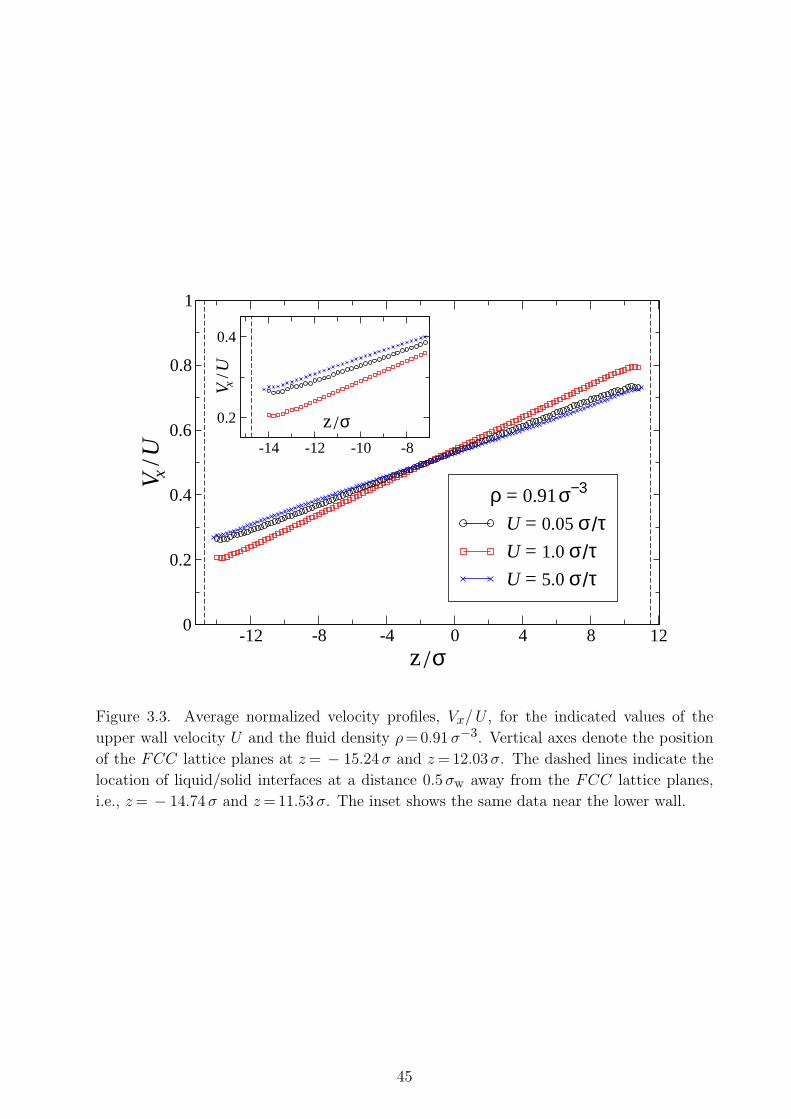
-12 -8 -4 0 4 8 12z/σ

0

0.2

0.4

0.6

0.8

1

V x/U -14 -12 -10 -8

z/σ0.2

0.4

V x/U

ρ = 0.91σ−3

U = 1.0 σ/τU = 5.0 σ/τ

U = 0.05 σ/τ

Figure 3.3. Average normalized velocity profiles, Vx/ U , for the indicated values of the

upper wall velocity U and the fluid density ρ = 0.91 σ−3. Vertical axes denote the position

of the FCC lattice planes at z = − 15.24 σ and z = 12.03 σ. The dashed lines indicate the

location of liquid/solid interfaces at a distance 0.5 σw away from the FCC lattice planes,

i.e., z = − 14.74 σ and z = 11.53 σ. The inset shows the same data near the lower wall.

45

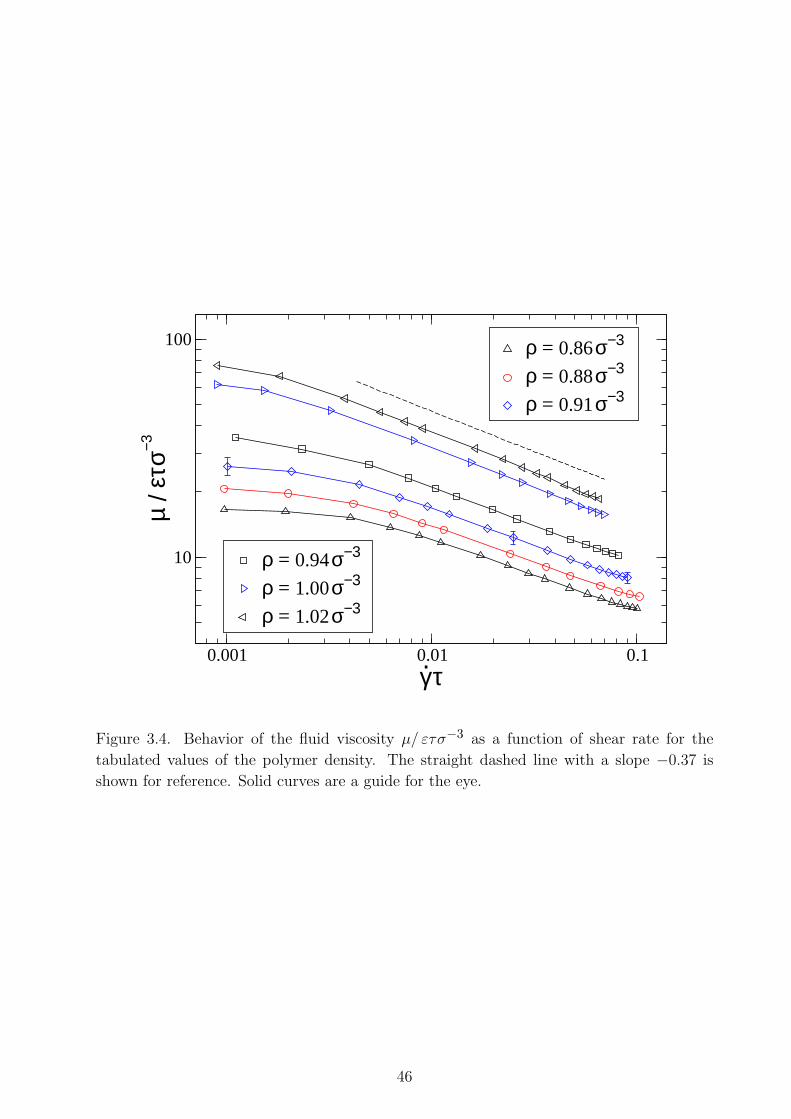
0.001 0.01 0.1γ.τ

10

100

µ / ε

τσ−3

ρ = 1.02σ−3ρ = 1.00σ−3ρ = 0.94σ−3

ρ = 0.91σ−3ρ = 0.88σ−3ρ = 0.86σ−3

Figure 3.4. Behavior of the fluid viscosity µ/ ετσ−3 as a function of shear rate for the

tabulated values of the polymer density. The straight dashed line with a slope −0.37 is

shown for reference. Solid curves are a guide for the eye.

46

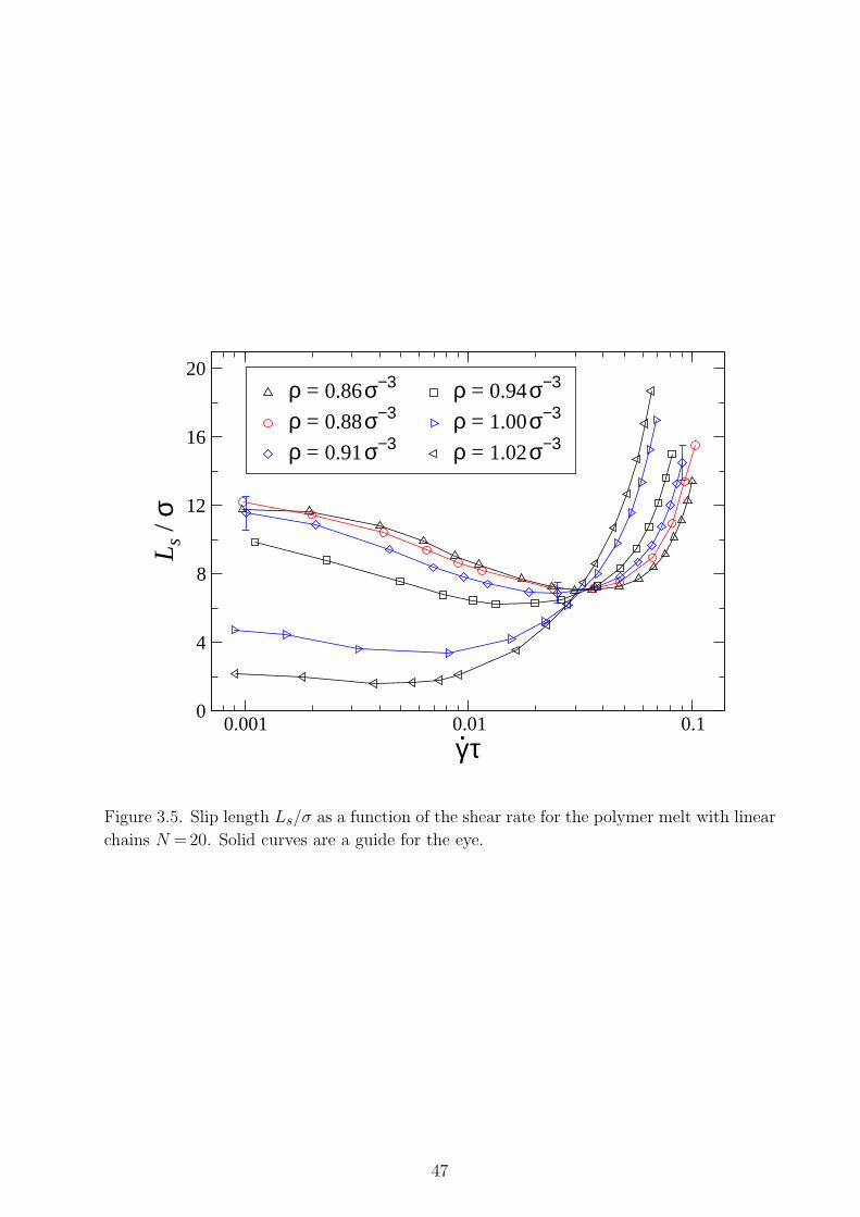
0.001 0.01 0.1

γ.τ

0

4

8

12

16

20

Ls /

σ

ρ = 0.86σ−3 ρ = 0.94σ−3

ρ = 0.88σ−3

ρ = 0.91σ−3ρ = 1.00σ−3

ρ = 1.02σ−3

Figure 3.5. Slip length Ls/σ as a function of the shear rate for the polymer melt with linear

chains N = 20. Solid curves are a guide for the eye.

47

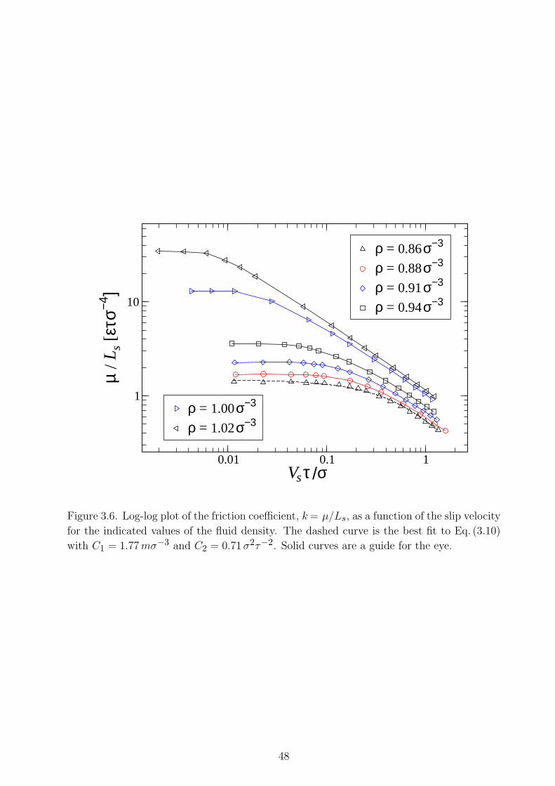
0.01 0.1 1Vsτ /σ

1

10

µ/L

s [ετ

σ−4]

ρ = 0.86σ−3

ρ = 0.88σ−3

ρ = 0.91σ−3

ρ = 0.94σ−3

ρ = 1.00σ−3

ρ = 1.02σ−3

Figure 3.6. Log-log plot of the friction coefficient, k = µ/Ls, as a function of the slip velocity

for the indicated values of the fluid density. The dashed curve is the best fit to Eq. (3.10)

with C1 = 1.77 mσ−3 and C2 = 0.71 σ2τ−2. Solid curves are a guide for the eye.

48

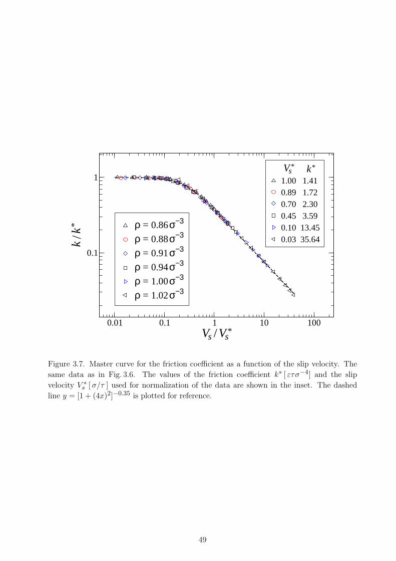
0.01 0.1 1 10 100Vs /Vs

*

0.1

1

k/k

*

ρ = 1.02σ−3ρ = 1.00σ−3ρ = 0.94σ−3ρ = 0.91σ−3ρ = 0.88σ−3ρ = 0.86σ−3

Vs* k*

1.00 1.41

0.70 2.30 0.89 1.72

0.45 3.590.10 13.450.03 35.64

Figure 3.7. Master curve for the friction coefficient as a function of the slip velocity. The

same data as in Fig. 3.6. The values of the friction coefficient k∗ [ ετσ−4] and the slip

velocity V ∗s [ σ/τ ] used for normalization of the data are shown in the inset. The dashed

line y = [1 + (4x)2]−0.35 is plotted for reference.

49

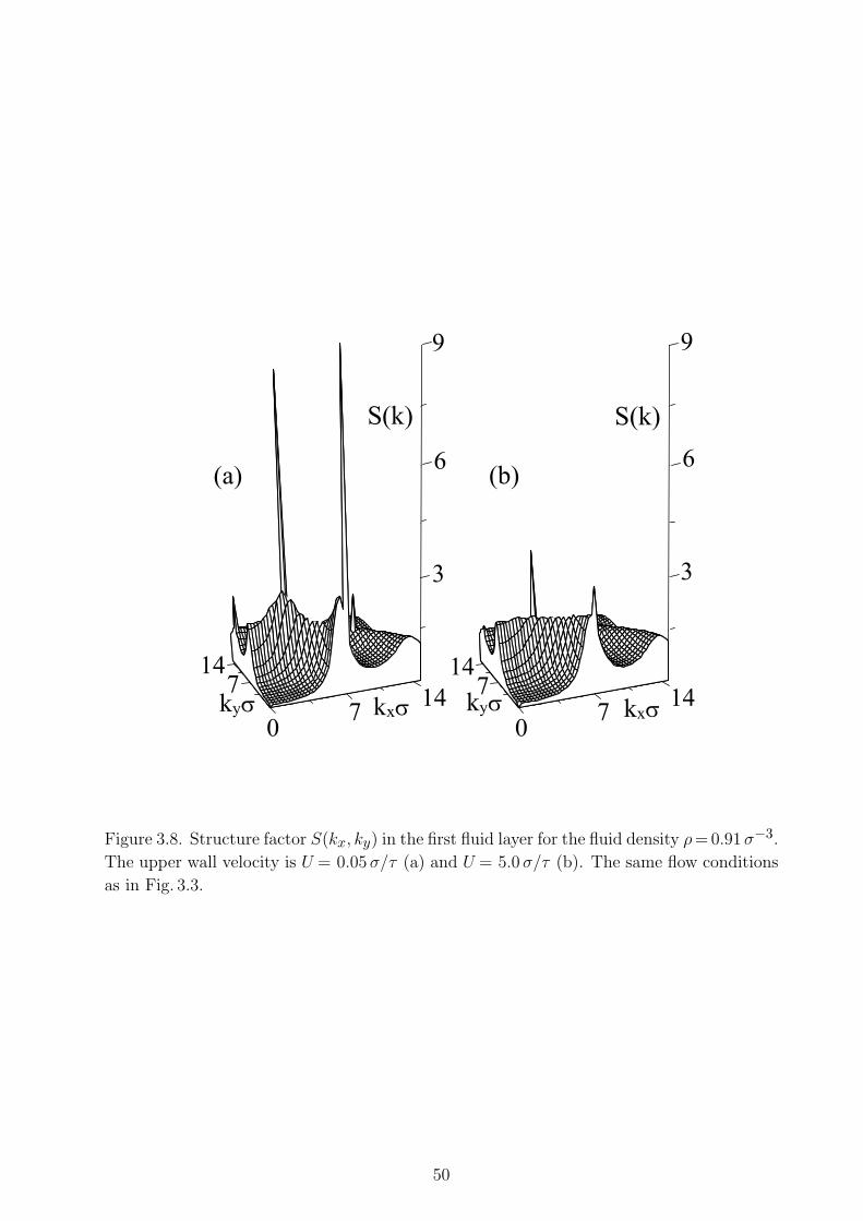
Figure 3.8. Structure factor S(kx, ky) in the first fluid layer for the fluid density ρ = 0.91 σ−3.

The upper wall velocity is U = 0.05 σ/τ (a) and U = 5.0 σ/τ (b). The same flow conditions

as in Fig. 3.3.

50

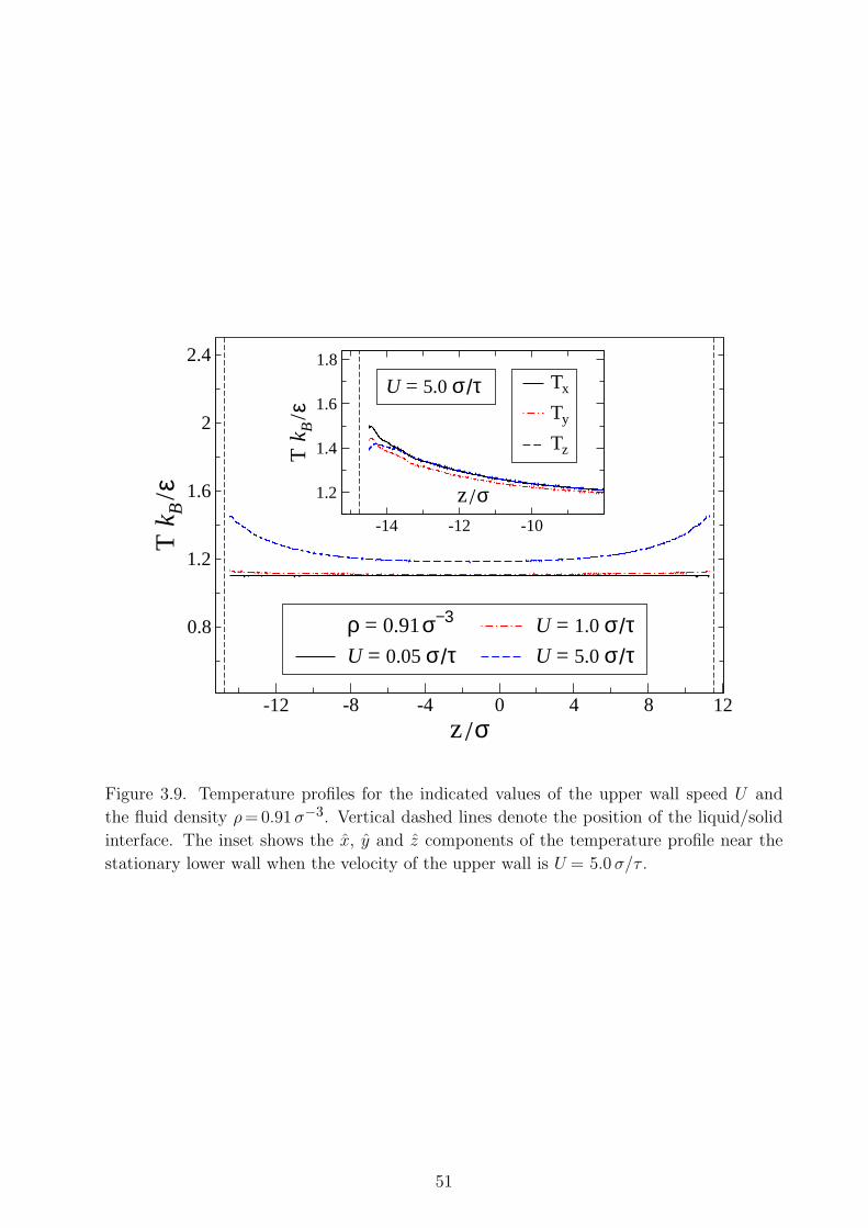
-12 -8 -4 0 4 8 12z/σ

0.8

1.2

1.6

2

2.4

Tk B

/ε

-14 -12 -10

z/σ1.2

1.4

1.6

1.8

Tk B

/ε

ρ = 0.91σ−3

U = 0.05 σ/τU = 1.0 σ/τU = 5.0 σ/τ

U = 5.0 σ/τ Tx

Ty

Tz

Figure 3.9. Temperature profiles for the indicated values of the upper wall speed U and

the fluid density ρ = 0.91 σ−3. Vertical dashed lines denote the position of the liquid/solid

interface. The inset shows the x, y and z components of the temperature profile near the

stationary lower wall when the velocity of the upper wall is U = 5.0 σ/τ .

51

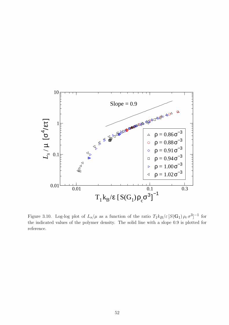
0.01 0.1 0.3

T1kB/ε [S(G1)ρcσ3]−1

0.01

0.1

1

10

Ls

/µ [

σ4 /ε

τ]

ρ = 0.86σ−3

ρ = 0.88σ−3

ρ = 0.91σ−3

ρ = 0.94σ−3

ρ = 1.00σ−3

ρ = 1.02σ−3

Slope = 0.9

Figure 3.10. Log-log plot of Ls/µ as a function of the ratio T1kB/ε [S(G1) ρc σ3]−1 for

the indicated values of the polymer density. The solid line with a slope 0.9 is plotted for

reference.

52

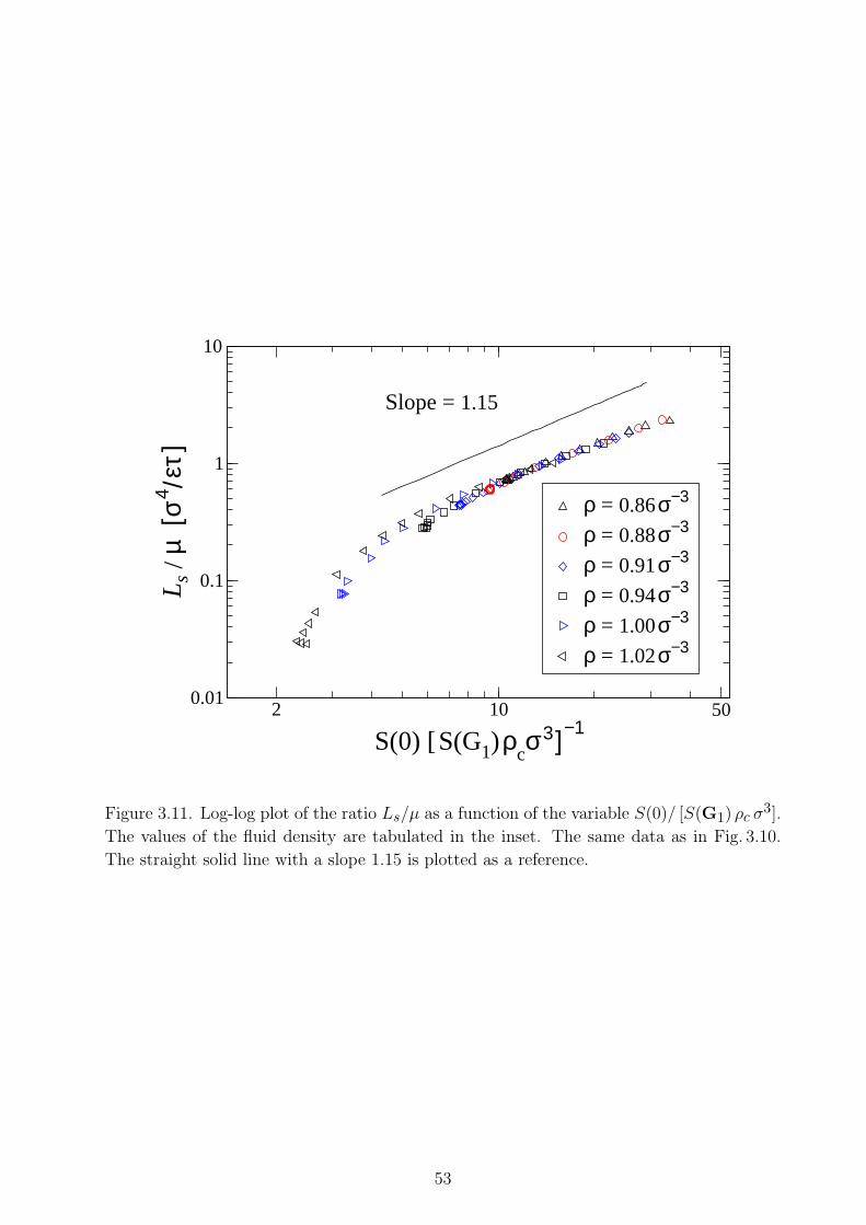
2 10 50

S(0) [S(G1)ρcσ3]−1

0.01

0.1

1

10

Ls

/µ [

σ4 /ε

τ]

ρ = 0.86σ−3

ρ = 0.88σ−3

ρ = 0.91σ−3

ρ = 0.94σ−3

ρ = 1.00σ−3

ρ = 1.02σ−3

Slope = 1.15

Figure 3.11. Log-log plot of the ratio Ls/µ as a function of the variable S(0)/ [S(G1) ρc σ3].

The values of the fluid density are tabulated in the inset. The same data as in Fig. 3.10.

The straight solid line with a slope 1.15 is plotted as a reference.

53

CHAPTER 4

The effective slip length and vortex

formation in laminar flow over a

rough surface

4.1 Introduction

An accurate flow prediction in micro-channels is important for the optimal design and

fabrication of microfluidic devices whose applications range from medicine to biotechnol-

ogy [81, 82]. The boundary conditions and the surface topology are major factors affecting

the flow pattern near the solid boundary and the formation of recirculation zones. The

flow separation at rough surfaces can modify the wall shear stress distribution or initiate

instability towards turbulence. In microfluidic channels, the vortex flow enhances the mix-

ing efficiency [83, 84] and promotes convective heat transfer [85, 86, 87]. In cardiovascular

systems, the separation region at the entrance of branching vessels may trap lipid particles

which could lead to arterial diseases [88, 89, 90]. In the present study we examine the role

of slip boundary condition in determining the flow properties near rough surfaces including

the separation phenomena, and distribution of pressure and shear stress along the surface.

Although the validity of the no-slip boundary condition is well accepted at the macro-

scopic level, recent experiments [5, 16, 9, 19, 91, 14] and molecular dynamics (MD) simu-

lations [21, 23, 25, 92, 27, 29] reported the existence of a boundary slip in microflows. The

54

model first proposed by Navier relates the slip velocity to the rate of shear via the propor-

tionality coefficient, the so-called slip length. The MD simulations are particularly suitable

for examining the influence of molecular parameters on the microscopic slip length at the

liquid/solid interface. The advantage of the MD simulations is that a detailed flow analysis

can be performed at the molecular level while the explicit specification of the boundary

conditions is not required. In contrast to description of the flow near boundary by means of

microscopic slip length, it is convenient to characterize the flow over macroscopically rough

surfaces by the effective slip length, which is defined as a distance from the level of the

mean height of the surface roughness to the point where linearly extrapolated bulk velocity

profile vanishes. Recent MD studies have demonstrated that the effective slip length in a

flow of simple fluids [35] and polymer melts [93] over a wavy surface agrees well with hydro-

dynamic predictions [51, 52] when the corrugation wavelength is larger than approximately

thirty molecular diameters.

The influence of surface roughness on fluid flow with either local no-slip or zero shear stress

(i.e. perfect slip) boundary conditions has been extensively studied in the past decades [43,

62, 94, 95, 63, 96, 97], see also a review section in [35]. Analytical calculations have shown

that in a shear flow over a corrugated surface with microscopic no-slip or zero shear stress

conditions, the effective boundary slip is insignificant macroscopically [43, 94]. The effective

no-slip boundary plane is located at the intermediate position between crests and valleys of

the rough surface when the no-slip condition is imposed along the solid boundary [62, 63,

98, 14, 36]. For an arbitrary surface roughness with small amplitudes, the slip coefficient

in the Navier model is proportional to the average amplitude of the wall roughness and

depends on the position of the origin of the coordinate system [95]. Applying the no-slip

boundary condition along the wavy surface, Tuck and Kouzoubov [63] have demonstrated

that the effective slip length is inversely proportional to the corrugation wavelength and

quadratically proportional to the amplitude of the surface roughness. However, the series

expansion method used in [63] fails at large wavenumbers, ka & 0.5, when a backflow

appears inside the grooves of the substrate. The effective slip length for a flow above the

surface with deep corrugations only weakly depends on the depth of the grooves [62, 97, 93].

Despite considerable analytical efforts, the relation between the vortex flow structure in

55

deep grooves and the effective slip length has not yet been systematically investigated.

The laminar flow separation at the corrugated surface with the local no-slip boundary

conditions depends on the depth of the grooves and the Reynolds number [99, 100, 101, 102,

103, 104, 105, 106]. In a creeping flow over a sinusoidal surface, the flow circulation appears

in sufficiently deep grooves and, as the corrugation amplitude increases, the vortex grows

and remains symmetric [104, 107, 108]. With increasing Reynolds number, the vortex flow

forms even in shallow grooves, the circulation region expands, and the center of vorticity is

displaced upstream [99, 102, 103, 105]. In the limit of small-scale surface roughness and for

no-slip boundary conditions, the apparent slip velocity at the mean surface becomes more

negative as the Reynolds number increases [63]. A noticeable change in the effective slip

length was also observed at Re & 100 for laminar flow over deep grooves when the local slip

length is comparable to the corrugation amplitude [93]. However, the influence of the local

slip condition at the curved boundary on the vortex flow formation has not been considered

at finite Reynolds numbers.

This chapter is focused on investigation of the effects of local slip boundary conditions and

the Reynolds number on the flow structure near periodically corrugated surfaces and the

effective slip length. We will show that for the Stokes flow with the local no-slip boundary

condition, the effective slip length decreases with increasing corrugation amplitude and

the flow circulation develops in sufficiently deep grooves. In the presence of the local slip

boundary condition along the rough surface, the effective slip length increases and the size of

the vortex is reduced but its structure remains symmetrical. The analysis of the numerical

solution of the Navier-Stokes equation with the local slip condition shows that the inertial

effects promote the asymmetric vortex flow formation and reduce the effective slip length.

This chapter is organized as follows. The details of a continuum model and the im-

plementation of the local slip boundary conditions are described in the next section. The

analytical results for the Stokes flow over a wavy surface by Panzer et al. [52] are summarized

in Sec. 4.3.1. The analysis of the effective slip length and the flow structure is presented in

Sec. 4.3.2 for the no-slip case and in Sec. 4.3.3 for the finite microscopic slip. The effect of

Reynolds number on the effective slip flow over a periodically corrugated surface is studied

in Sec. 4.3.4. A brief summary is given in the last section.

56

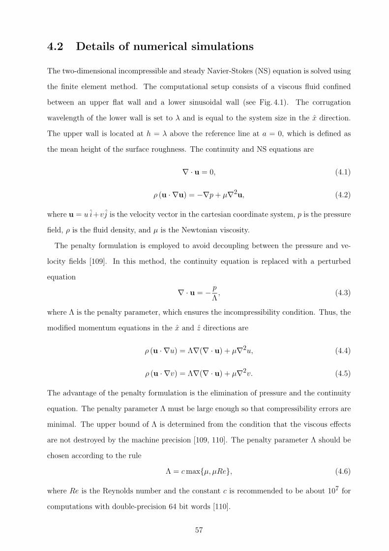
4.2 Details of numerical simulations

The two-dimensional incompressible and steady Navier-Stokes (NS) equation is solved using

the finite element method. The computational setup consists of a viscous fluid confined

between an upper flat wall and a lower sinusoidal wall (see Fig. 4.1). The corrugation

wavelength of the lower wall is set to λ and is equal to the system size in the x direction.

The upper wall is located at h = λ above the reference line at a = 0, which is defined as

the mean height of the surface roughness. The continuity and NS equations are

∇ · u = 0, (4.1)

ρ (u · ∇u) = −∇p + µ∇2u, (4.2)

where u = u i+vj is the velocity vector in the cartesian coordinate system, p is the pressure

field, ρ is the fluid density, and µ is the Newtonian viscosity.

The penalty formulation is employed to avoid decoupling between the pressure and ve-

locity fields [109]. In this method, the continuity equation is replaced with a perturbed

equation

∇ · u = − p

Λ, (4.3)

where Λ is the penalty parameter, which ensures the incompressibility condition. Thus, the

modified momentum equations in the x and z directions are

ρ (u · ∇u) = Λ∇(∇ · u) + µ∇2u, (4.4)

ρ (u · ∇v) = Λ∇(∇ · u) + µ∇2v. (4.5)

The advantage of the penalty formulation is the elimination of pressure and the continuity

equation. The penalty parameter Λ must be large enough so that compressibility errors are

minimal. The upper bound of Λ is determined from the condition that the viscous effects

are not destroyed by the machine precision [109, 110]. The penalty parameter Λ should be

chosen according to the rule

Λ = c maxµ, µRe, (4.6)

where Re is the Reynolds number and the constant c is recommended to be about 107 for

computations with double-precision 64 bit words [110].

57

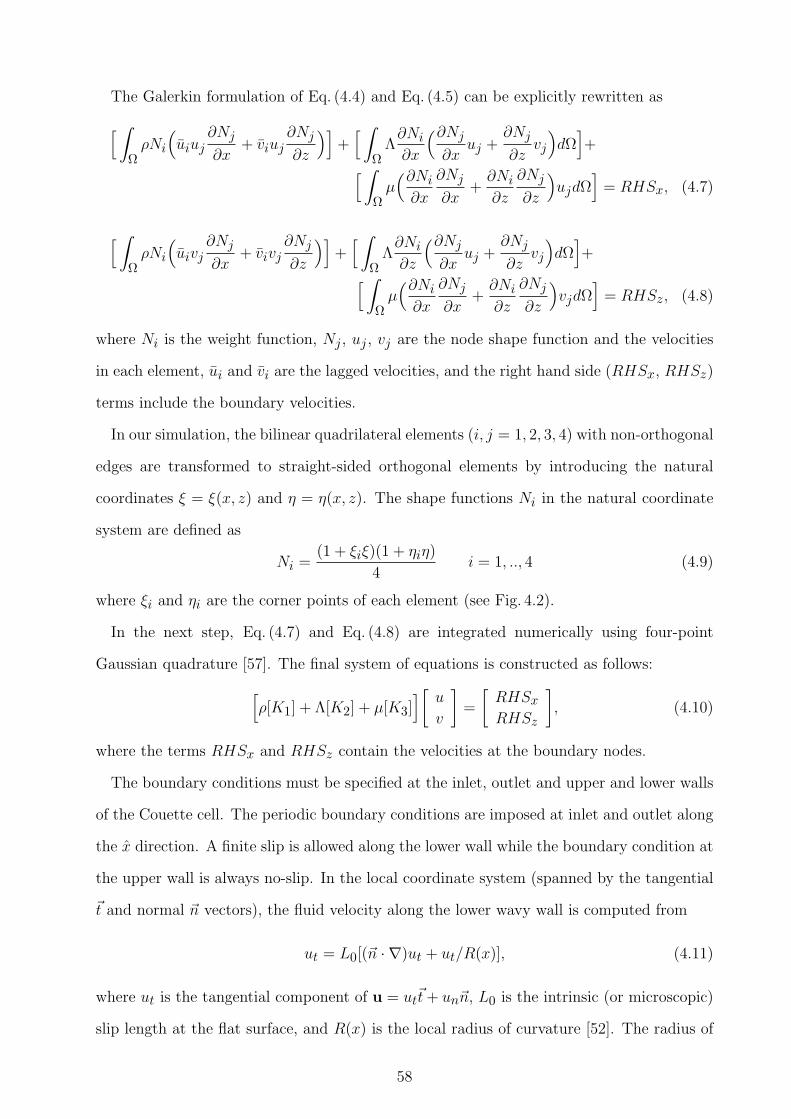
The Galerkin formulation of Eq. (4.4) and Eq. (4.5) can be explicitly rewritten as

[ ∫

ΩρNi

(uiuj

∂Nj

∂x+ viuj

∂Nj

∂z

)]+

[ ∫

ΩΛ

∂Ni

∂x

(∂Nj

∂xuj +

∂Nj

∂zvj

)dΩ

]+

[ ∫

Ωµ(∂Ni

∂x

∂Nj

∂x+

∂Ni

∂z

∂Nj

∂z

)ujdΩ

]= RHSx, (4.7)

[ ∫

ΩρNi

(uivj

∂Nj

∂x+ vivj

∂Nj

∂z

)]+

[ ∫

ΩΛ

∂Ni

∂z

(∂Nj

∂xuj +

∂Nj

∂zvj

)dΩ

]+

[ ∫

Ωµ(∂Ni

∂x

∂Nj

∂x+

∂Ni

∂z

∂Nj

∂z

)vjdΩ

]= RHSz, (4.8)

where Ni is the weight function, Nj , uj , vj are the node shape function and the velocities

in each element, ui and vi are the lagged velocities, and the right hand side (RHSx, RHSz)

terms include the boundary velocities.

In our simulation, the bilinear quadrilateral elements (i, j = 1, 2, 3, 4) with non-orthogonal

edges are transformed to straight-sided orthogonal elements by introducing the natural

coordinates ξ = ξ(x, z) and η = η(x, z). The shape functions Ni in the natural coordinate

system are defined as

Ni =(1 + ξiξ)(1 + ηiη)

4i = 1, .., 4 (4.9)

where ξi and ηi are the corner points of each element (see Fig. 4.2).

In the next step, Eq. (4.7) and Eq. (4.8) are integrated numerically using four-point

Gaussian quadrature [57]. The final system of equations is constructed as follows:

[ρ[K1] + Λ[K2] + µ[K3]

][ u

v

]=

[RHSx

RHSz

], (4.10)

where the terms RHSx and RHSz contain the velocities at the boundary nodes.

The boundary conditions must be specified at the inlet, outlet and upper and lower walls

of the Couette cell. The periodic boundary conditions are imposed at inlet and outlet along

the x direction. A finite slip is allowed along the lower wall while the boundary condition at

the upper wall is always no-slip. In the local coordinate system (spanned by the tangential

~t and normal ~n vectors), the fluid velocity along the lower wavy wall is computed from

ut = L0[(~n · ∇)ut + ut/R(x)], (4.11)

where ut is the tangential component of u = ut~t + un~n, L0 is the intrinsic (or microscopic)

slip length at the flat surface, and R(x) is the local radius of curvature [52]. The radius of

58

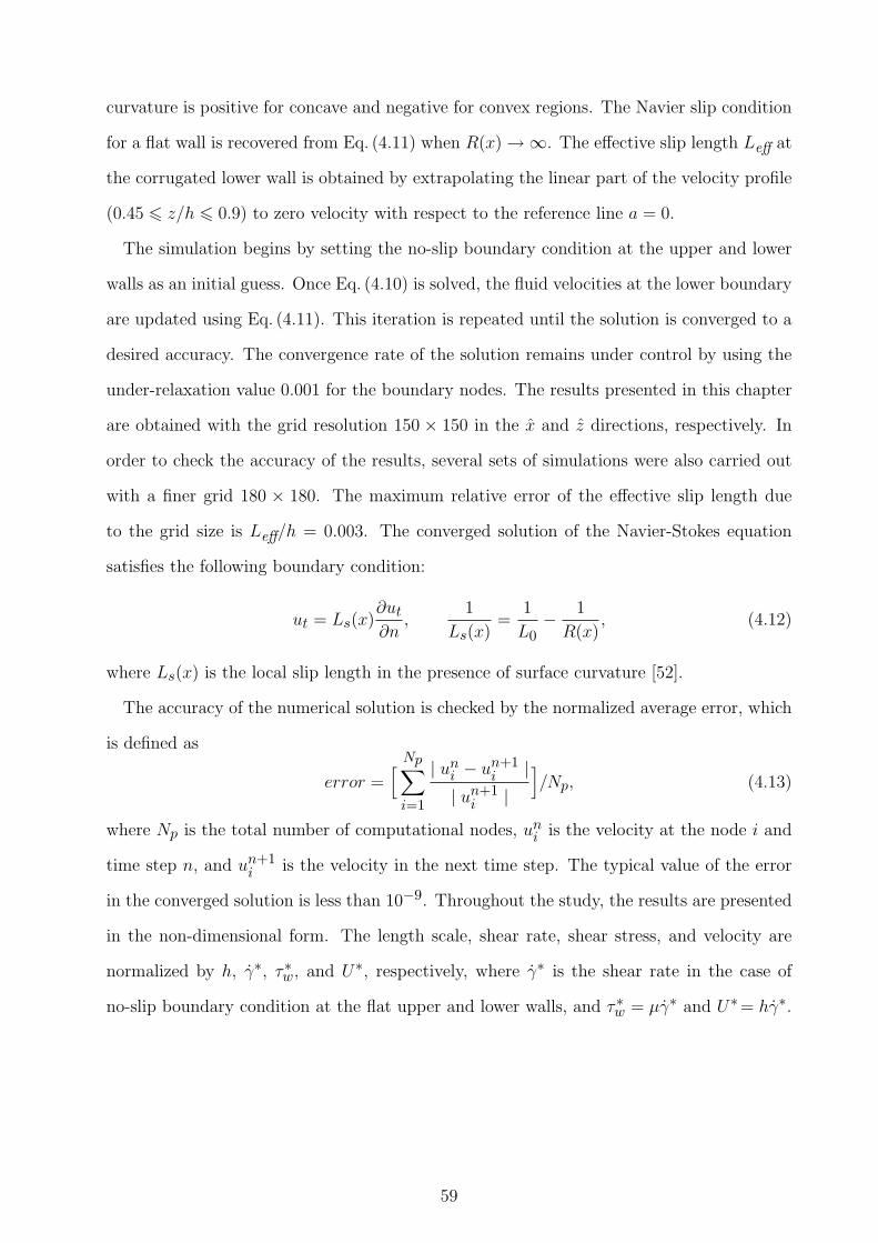
curvature is positive for concave and negative for convex regions. The Navier slip condition

for a flat wall is recovered from Eq. (4.11) when R(x) →∞. The effective slip length Leff at

the corrugated lower wall is obtained by extrapolating the linear part of the velocity profile

(0.45 6 z/h 6 0.9) to zero velocity with respect to the reference line a = 0.

The simulation begins by setting the no-slip boundary condition at the upper and lower

walls as an initial guess. Once Eq. (4.10) is solved, the fluid velocities at the lower boundary

are updated using Eq. (4.11). This iteration is repeated until the solution is converged to a

desired accuracy. The convergence rate of the solution remains under control by using the

under-relaxation value 0.001 for the boundary nodes. The results presented in this chapter

are obtained with the grid resolution 150 × 150 in the x and z directions, respectively. In

order to check the accuracy of the results, several sets of simulations were also carried out

with a finer grid 180 × 180. The maximum relative error of the effective slip length due

to the grid size is Leff/h = 0.003. The converged solution of the Navier-Stokes equation

satisfies the following boundary condition:

ut = Ls(x)∂ut

∂n,

1

Ls(x)=

1

L0− 1

R(x), (4.12)

where Ls(x) is the local slip length in the presence of surface curvature [52].

The accuracy of the numerical solution is checked by the normalized average error, which

is defined as

error =[ Np∑

i=1

| uni − un+1

i || un+1

i |]/Np, (4.13)

where Np is the total number of computational nodes, uni is the velocity at the node i and

time step n, and un+1i is the velocity in the next time step. The typical value of the error

in the converged solution is less than 10−9. Throughout the study, the results are presented

in the non-dimensional form. The length scale, shear rate, shear stress, and velocity are

normalized by h, γ∗, τ∗w, and U∗, respectively, where γ∗ is the shear rate in the case of

no-slip boundary condition at the flat upper and lower walls, and τ∗w = µγ∗ and U∗= hγ∗.

59

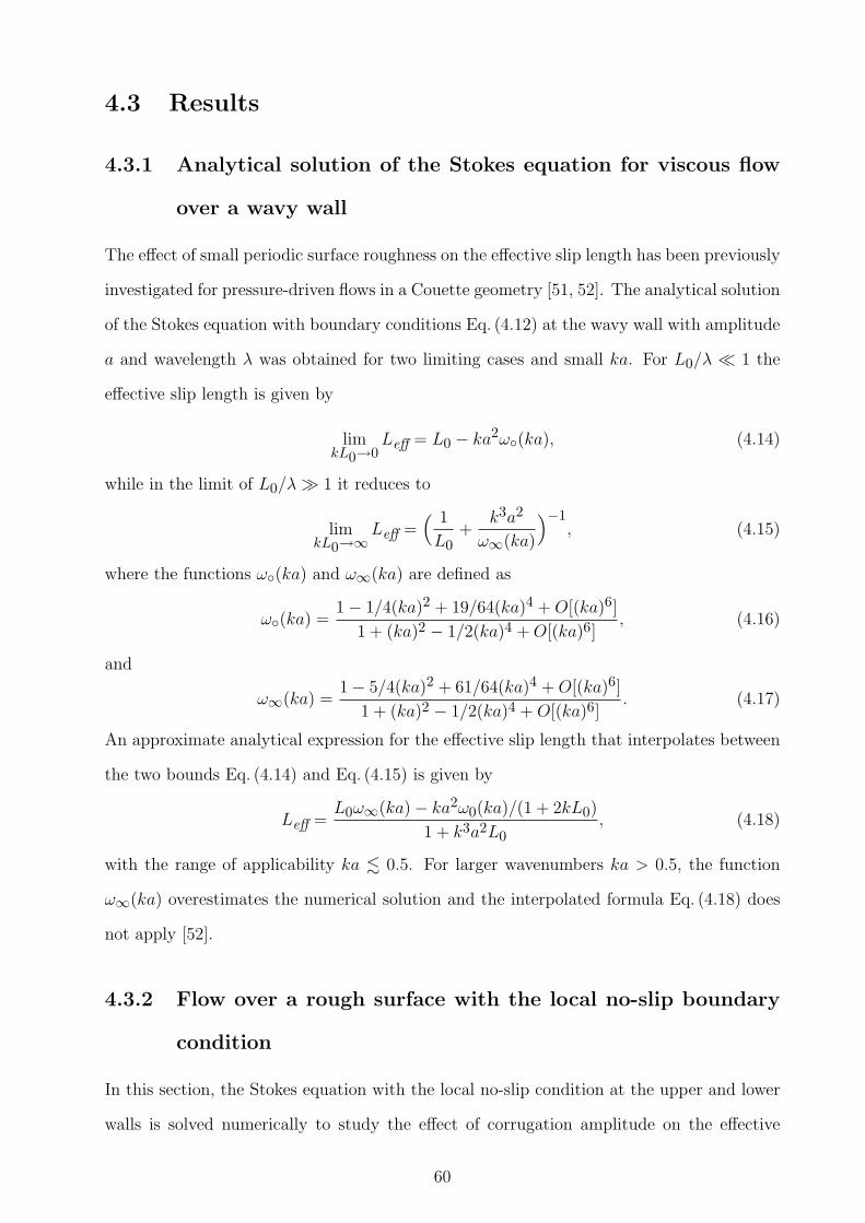
4.3 Results

4.3.1 Analytical solution of the Stokes equation for viscous flow

over a wavy wall

The effect of small periodic surface roughness on the effective slip length has been previously

investigated for pressure-driven flows in a Couette geometry [51, 52]. The analytical solution

of the Stokes equation with boundary conditions Eq. (4.12) at the wavy wall with amplitude

a and wavelength λ was obtained for two limiting cases and small ka. For L0/λ ¿ 1 the

effective slip length is given by

limkL0→0

Leff = L0 − ka2ω(ka), (4.14)

while in the limit of L0/λ À 1 it reduces to

limkL0→∞

Leff =( 1

L0+

k3a2

ω∞(ka)

)−1, (4.15)

where the functions ω(ka) and ω∞(ka) are defined as

ω(ka) =1− 1/4(ka)2 + 19/64(ka)4 + O[(ka)6]

1 + (ka)2 − 1/2(ka)4 + O[(ka)6], (4.16)

and

ω∞(ka) =1− 5/4(ka)2 + 61/64(ka)4 + O[(ka)6]

1 + (ka)2 − 1/2(ka)4 + O[(ka)6]. (4.17)

An approximate analytical expression for the effective slip length that interpolates between

the two bounds Eq. (4.14) and Eq. (4.15) is given by

Leff =L0ω∞(ka)− ka2ω0(ka)/(1 + 2kL0)

1 + k3a2L0, (4.18)

with the range of applicability ka . 0.5. For larger wavenumbers ka > 0.5, the function

ω∞(ka) overestimates the numerical solution and the interpolated formula Eq. (4.18) does

not apply [52].

4.3.2 Flow over a rough surface with the local no-slip boundary

condition

In this section, the Stokes equation with the local no-slip condition at the upper and lower

walls is solved numerically to study the effect of corrugation amplitude on the effective

60

slip length. The velocity profiles, averaged over the period of corrugation λ, are plotted

in the inset of Fig. 4.3 for several values of wavenumber ka = 2 πa/λ. As ka increases, the

normalized velocity profiles remain linear in the bulk region and become curved near the

lower corrugated wall. The linear part of the velocity profiles is used to compute the effective

slip length, which is plotted as a function of wavenumber in Fig. 4.3. With increasing

corrugation amplitude of the lower wall, the effective slip length decays monotonically and

becomes negative, indicating that the effective no-slip boundary is shifted into the fluid

domain. For ka . 1, the numerical results agree well with the analytical solution Eq. (4.18)

denoted by the solid line in Fig. 4.3. The deviation from the analytical solution becomes

significant at larger wavenumbers where the streamlines extracted from the Stokes solution

indicate the presence of backflow at the bottom of the valley.

In order to investigate the flow behavior above the sinusoidal surface, the shear stress and

pressure along the lower wall were computed from the solution of the Stokes equation. In

the presence of surface curvature the wall shear stress τw has two components

τw = µ(∂ut

∂n+ ut/R(x)

)∣∣∣w, (4.19)

where ∂ut/∂n is the normal derivative of the tangential velocity ut, and R(x) is the local

radius of curvature. In the case of no-slip boundary condition (ut = 0), the local shear

stress at the wall is reduced to τw = µ∂ut∂n . The normalized shear stress along the lower

corrugated wall is plotted in Fig. 4.4 for different corrugation amplitudes. The maximum

value of the shear stress is located at the peak of the surface corrugation (x/λ = 0.25)

and it increases with increasing amplitude, which is consistent with the results of previous

analytical studies of a laminar flow over a wavy wall [111, 100]. The fluid tangential velocity

near the boundary is proportional to the wall shear stress shown in Fig. 4.4. Therefore, the

tangential velocity is also maximum above the peak and, as the flow moves downstream, it

decelerates and the velocity becomes zero inside the valley at sufficiently large amplitudes.

For ka > 0.79, the shear stress profiles intersect the dashed line (τw = 0) at two points and a

clockwise flow circulation develops inside the valley. As the corrugation amplitude increases,

the intersection points move away from each other and the flow recirculation region becomes

larger. These results are in agreement with previous estimates of the critical wavenumber

61

ka ≈ 0.77 for the onset of flow separation in sufficiently thick films [107, 108].

The pressure along the lower wavy wall is plotted in Fig. 4.5 for the same amplitudes as

in Fig. 4.4. The value P ∗ used for normalization is the maximum pressure, which is located

above the wavy surface with ka = 1.12 on the left side of the peak. For each wavenumber,

the pressure along the surface is maximum on the left side of the peak, where the surface

faces the mainstream flow. The surface pressure reaches its minimum value on the right

side of the peak (see Fig. 4.5). As the flow moves further downstream into the valley, it

encounters an adverse pressure gradient, which becomes larger as ka increases. At large

wavenumbers ka > 0.83, the flow near the surface cannot overcome the combined resistance

of the viscous forces and the adverse pressure gradient, and separates from the surface at

the point where τw = 0.

The pressure contours and streamlines near the corrugated surface with wavenumber

ka = 1.12 are depicted in Fig. 4.6(a). The pressure contours indicate the presence of an

adverse pressure gradient in the region 0.3 . x/λ . 0.6 on the right side of the peak (see

also Fig. 4.5). The streamlines illustrate the flow separation inside the valley at x/λ ' 0.52.

After the separation point the flow near the wall reverses direction and moves against the

mainstream. The local velocity profile inside the valley is shown in the inset of Fig. 4.6(a).

As the flow cross-section decreases towards the peak, the flow attaches to the surface at

the point where the shear stress is zero again. Note also that for ka > 0.83 in Fig. 4.5, the

pressure profiles along the lower surface exhibit a slight drop inside the valley where the

vortex is present. After the attachment point, due to the periodic boundary condition in

the x direction, the surface pressure increases up to its maximum value, which is located on

the left side of the peak. The nonlinearity due to inertia is absent in the Stokes flow and

the vortex in the valley remains symmetrical.

We also comment that a secondary vortex is formed inside a deeper cavity (ka ≈ 2.33),

which is counter-rotating with respect to the primary vortex (not shown). Previous analyti-

cal study of a creeping flow over a wavy wall demonstrated that a secondary vortex appears

at ka & 2.28 when the channel width is larger than the corrugation wavelength [108]. In

the limiting case, when the cavity consists of two parallel walls, an infinite sequence of

counter-rotating vortices appears between the walls [112, 113].

62

4.3.3 Effect of the local slip on the flow pattern near the rough

surface

Next, we present the results of the numerical solution of the Stokes equation with the

local slip condition at the lower wavy wall while the boundary condition at the upper

wall remains no-slip. The pressure contours and the streamlines are plotted in Fig. 4.6 for

several values of the intrinsic slip length L0 and the wavenumber ka = 1.12. The streamline

patterns indicate that with increasing slip length L0, the size of vortex inside the valley is

progressively reduced and the vortex eventually disappears. Similar to the analysis in the

previous section, the pressure and shear stress along the lower wall are computed in the

presence of the local boundary slip.

The normalized pressure along the lower wavy wall is plotted in Fig. 4.7 as a function of

the slip length L0. Similar to the case of no-slip boundary condition, the profiles exhibit a

maximum and a minimum in pressure on the right and left sides on the peak, respectively.

In a wide range of L0, the difference between the locations and the magnitudes of the

extrema is barely noticeable. As the flow moves down a slope (0.3 . x/λ . 0.5 region

in Fig. 4.7), the pressure gradient along the surface becomes positive and its magnitude

decreases with increasing values of L0. The separation and attachment points are located

at the intersection of the shear stress profiles with the horizontal line (τw = 0) shown in

Fig. 4.8. In comparison to the no-slip case, the smaller combined effect of the adverse

pressure gradient and the wall shear stress causes a shift of the separation point deeper into

the valley (e.g. see Fig. 4.6). As the slip length L0 increases, the separation and attachment

points move closer to each other, the vortex becomes smaller and eventually vanishes. We

also note that at the separation point both components of the shear stress ∂ut/∂n and

ut/R(x) become zero in agreement with the MRS criterion for the flow separation of the

boundary layer at a moving substrate [114].

The influence of the local slip on the shape of the velocity profile and the normal derivative

of the tangential velocity at the bottom of the valley is illustrated in the insets of Fig. 4.6.

The local slip length Ls(x) in Eq. (4.12) is a function of the radius of curvature R(x) and

the intrinsic slip length L0. For all cases considered in Fig. 4.6, the condition L0 < |R(x)|

63

holds and the local slip length Ls remains positive everywhere along the lower wall, which

means that the slip velocity ut and the normal derivative ∂ut/∂n carry the same sign. It is

expected, however, that for the opposite condition, L0 > |R(x)|, the values ut and ∂ut/∂n

would have different signs at the bottom of the valley, and the corresponding velocity profile

will be qualitatively similar to the profile shown in the inset of Fig. 4.6(d) but shifted by a

negative slip velocity (see next section).

The effective slip length computed from the numerical solution of the Stokes equation and

Eq. (4.18) is plotted in Fig. 4.9 as a function of the intrinsic slip length L0 for wavenumbers

ka = 0.28 (a/h = 0.04) and ka = 1.12 (a/h = 0.18). For small values of L0, the effective

slip length approaches a negative value previously reported in Fig. 4.3 for the no-slip case.

As L0 increases, Leff grows monotonically and appears to saturate to a constant value. The

transition of the effective slip length from a growing function of L0 to a nearly constant

value occurs at larger L0 when ka decreases. For the small wavenumber ka = 0.28, the

effective slip length computed from Eq. (4.18) is in a good agreement with the numerical

solution of the Stokes equation. Visual inspection of the streamline patterns indicates

that there is no backflow at any L0. In the saturation regime, L0 →∞, the wall shear

stress becomes zero everywhere along the lower boundary, the streamlines near the lower

wall follow the boundary curvature, and the effective slip length in Eq. (4.15) approaches

Leff/λ ' 1/ [2π(ka)2] − 9/8π. For the large wavenumber ka = 1.12, the analytical results

Eq. (4.18) overestimate Leff computed from the numerical solution at L0/h & 0.02 and the

flow circulation is developed in the valley at L0/h 6 0.067. The vortex vanishes at the

bottom of the valley at sufficiently large values of L0 (denoted by the vertical arrow in

Fig. 4.9), and the flow streamlines are deformed to follow the boundary curvature [e.g. see

Fig. 4.6(d)]. The results for the intrinsic slip length, which determines the threshold for

the onset of the flow circulation at the bottom of the groove, are summarized in Fig. 4.10.

For the wavenumbers examined in this study, ka 6 1.26, the numerical simulations indicate

that if the flow circulation is present in the valley then the effective slip length is negative

and Leff increases with decreasing vortex size.

64

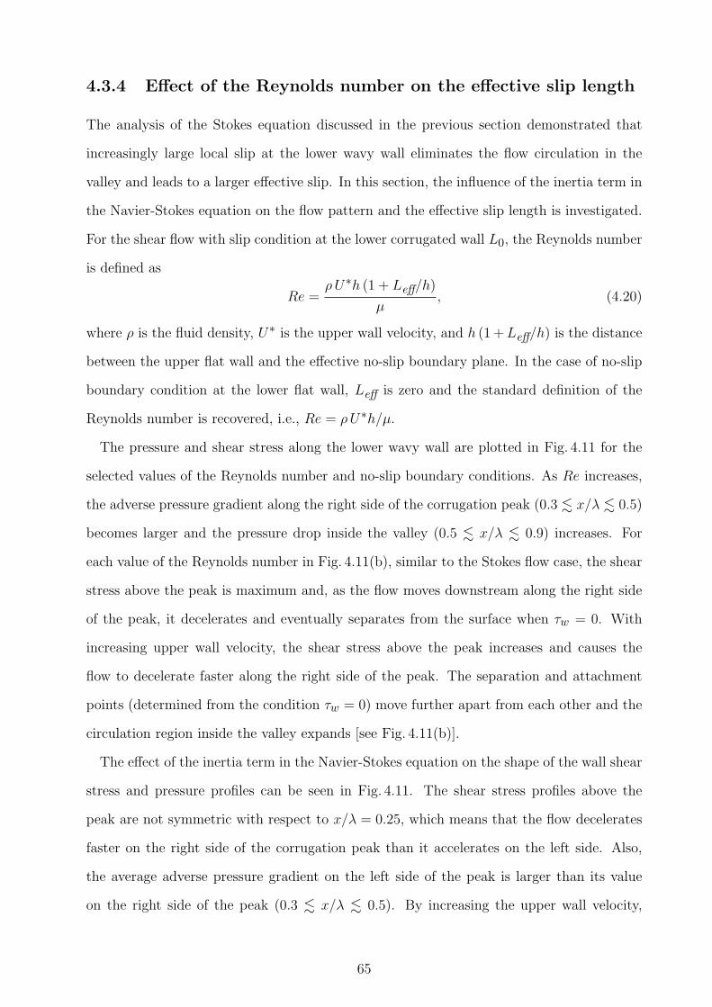
4.3.4 Effect of the Reynolds number on the effective slip length

The analysis of the Stokes equation discussed in the previous section demonstrated that

increasingly large local slip at the lower wavy wall eliminates the flow circulation in the

valley and leads to a larger effective slip. In this section, the influence of the inertia term in

the Navier-Stokes equation on the flow pattern and the effective slip length is investigated.

For the shear flow with slip condition at the lower corrugated wall L0, the Reynolds number

is defined as

Re =ρU∗h (1 + Leff/h)

µ, (4.20)

where ρ is the fluid density, U∗ is the upper wall velocity, and h (1 + Leff/h) is the distance

between the upper flat wall and the effective no-slip boundary plane. In the case of no-slip

boundary condition at the lower flat wall, Leff is zero and the standard definition of the

Reynolds number is recovered, i.e., Re = ρU∗h/µ.

The pressure and shear stress along the lower wavy wall are plotted in Fig. 4.11 for the

selected values of the Reynolds number and no-slip boundary conditions. As Re increases,

the adverse pressure gradient along the right side of the corrugation peak (0.3 . x/λ . 0.5)

becomes larger and the pressure drop inside the valley (0.5 . x/λ . 0.9) increases. For

each value of the Reynolds number in Fig. 4.11(b), similar to the Stokes flow case, the shear

stress above the peak is maximum and, as the flow moves downstream along the right side

of the peak, it decelerates and eventually separates from the surface when τw = 0. With

increasing upper wall velocity, the shear stress above the peak increases and causes the

flow to decelerate faster along the right side of the peak. The separation and attachment

points (determined from the condition τw = 0) move further apart from each other and the

circulation region inside the valley expands [see Fig. 4.11(b)].

The effect of the inertia term in the Navier-Stokes equation on the shape of the wall shear

stress and pressure profiles can be seen in Fig. 4.11. The shear stress profiles above the

peak are not symmetric with respect to x/λ = 0.25, which means that the flow decelerates

faster on the right side of the corrugation peak than it accelerates on the left side. Also,

the average adverse pressure gradient on the left side of the peak is larger than its value

on the right side of the peak (0.3 . x/λ . 0.5). By increasing the upper wall velocity,

65

the separation point moves further upstream than the attachment point downstream. The

formation of asymmetric vortex flow at finite Reynolds numbers is consistent with previous

findings for a flow in an undulated tube [103, 99, 102, 105]. The pressure contours and

streamlines extracted from the NS equation with the no-slip boundary condition are plotted

in Fig. 4.12(a) for ka = 1.12 and Re = 79. The flow streamlines in the valley indicate an

asymmetric clockwise circulation, which is larger than the flow circulation region shown in

Fig. 4.6(a) for the Stokes case.

In the presence of the local slip condition along the lower corrugated wall, the size of the

vortex becomes smaller while the flow structure remains asymmetric (see Fig. 4.12). The

decrease of the vortex size is similar to the case of the Stokes flow shown in Fig. 4.6 and

can also be described in terms of the pressure and shear stress along the lower wall. In

Fig. 4.13 the pressure and shear stress profiles are plotted for the same values of the upper

wall velocity as in Fig. 4.11 but with the slip boundary condition (L0/h = 0.25) along the

lower wall. Note that the Reynolds numbers in Fig. 4.13 are slightly larger than the values

reported in Fig. 4.11 for the same U∗ because of the larger effective slip length entering

the definition of the Reynolds number [see Eq. (4.20)]. For each value of the upper wall

velocity, the adverse pressure gradient and the wall shear stress on the right side of the

peak are smaller than in the case of the no-slip boundary condition, and, as a result, the

vortex either becomes smaller or vanishes (see Figs. 4.11 and 4.13). As the Reynolds number

increases, however, the vortex forms and expands asymmetrically to fill the bottom of the

groove. The inset of the Fig. 4.12(b) demonstrates that the slip velocity at the bottom of the

valley is negative while its normal derivative ∂ut/∂n is positive, in contrast to the velocity

profiles shown in Fig. 4.6 for the same ka = 1.12 and smaller slip lengths L0/h 6 0.08.

The effective slip length is plotted in Fig. 4.14 as a function of the Reynolds number for

the selected values of the intrinsic slip length L0 and ka = 1.12. With increasing Reynolds

number, the flow streamlines move away from the lower boundary and straighten out, the

slope of the normalized velocity profiles increases and the effective no-slip boundary plane

is shifted into the fluid domain. For L0/h 6 0.067, the circulation is always present in

the valley and the flow streamlines in the bulk of the fluid do not penetrate deep into the

valley [e.g. see Fig. 4.12(b)]. For larger slip lengths L0/h > 0.067, the flow streamlines show

66

that there is no backflow at low Re, and the vortex is formed at the bottom of the valley

only at sufficiently large Reynolds numbers indicated by the dashed line in Fig. 4.14. The

numerical results obtained from the solution of the Navier-Stokes equation demonstrate that

the growth or decay of the vortex as a function of the Reynolds number or the intrinsic slip

length is accompanied by the decrease or increase of the effective slip length.

4.4 Conclusions

In this chapter the effects of local slip boundary condition and the Reynolds number on

the flow structure near sinusoidally corrugated surfaces and the effective slip length were

investigated numerically by solving the Stokes and Navier-Stokes equations. The effective

slip length was defined with respect to the mean height of the surface roughness by extrap-

olating the linear part of the velocity profile averaged over the corrugation period. In the

case of the Stokes flow with the local no-slip boundary condition, the effective slip length

decreases with increasing corrugation amplitude and the vortex flow develops in the groove

of the rough surface for ka > 0.79. In the presence of the local slip boundary condition

along the wavy wall, the effective slip length increases and the size of the recirculation zone

is reduced. The vortex vanishes at sufficiently large values of the intrinsic slip length. The

analysis of the pressure and wall shear stress computed from the Navier-Stokes equation

shows that the asymmetric vortex flow develops in the groove due to the inertia term even

when the local slip boundary condition is applied. The effective slip length decreases with

increasing Reynolds number. The numerical simulations suggest that the variation of the

vortex size as a function of either the Reynolds number or the intrinsic slip length correlates

with the magnitude of the effective slip length.

67

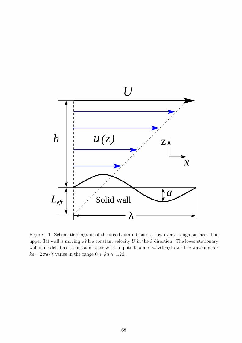
z

x

Solid wall

λL

z( )u

a

U

eff

h

Figure 4.1. Schematic diagram of the steady-state Couette flow over a rough surface. The

upper flat wall is moving with a constant velocity U in the x direction. The lower stationary

wall is modeled as a sinusoidal wave with amplitude a and wavelength λ. The wavenumber

ka = 2 πa/λ varies in the range 0 6 ka 6 1.26.

68

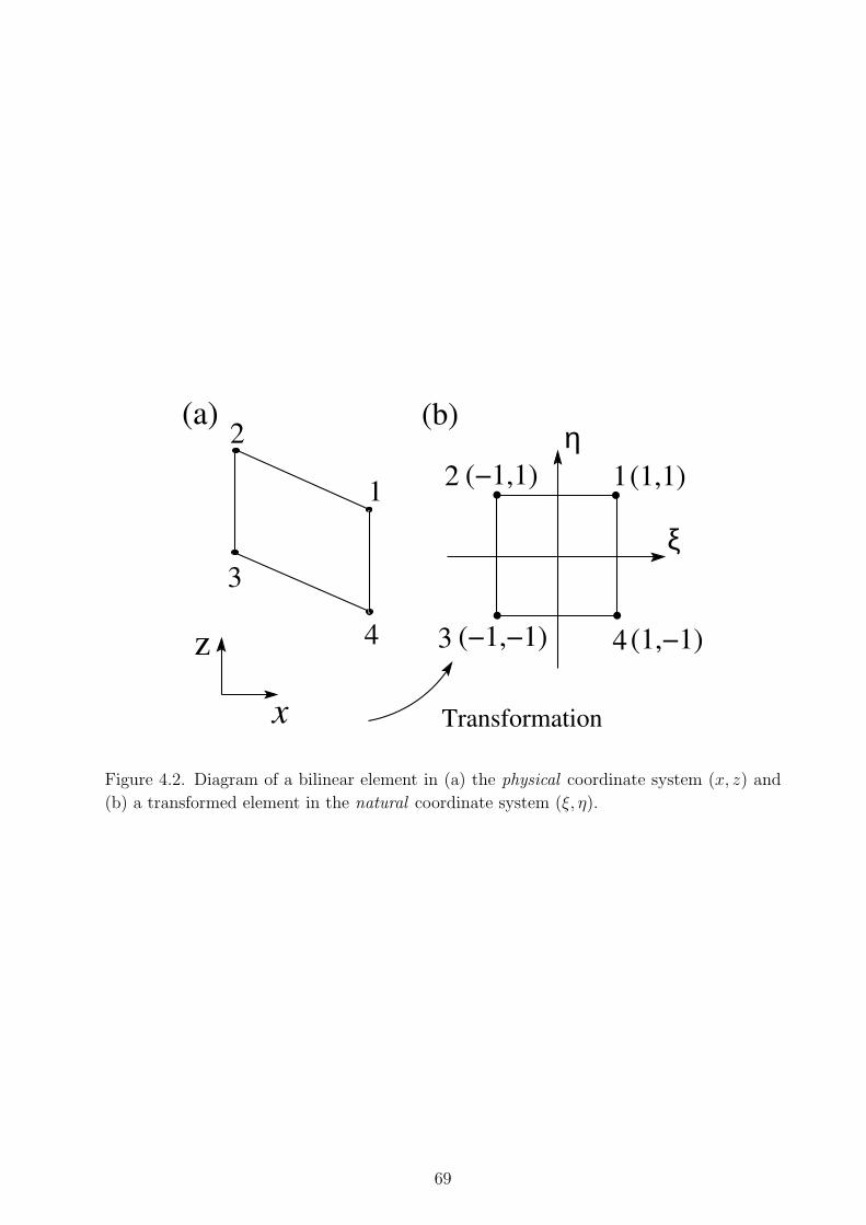
1

3

2

4

x

z

(a)

Transformation

ξ

η1(1,1)

3 (−1,−1)

2

4(1,−1)

(−1,1)

(b)

Figure 4.2. Diagram of a bilinear element in (a) the physical coordinate system (x, z) and

(b) a transformed element in the natural coordinate system (ξ, η).

69

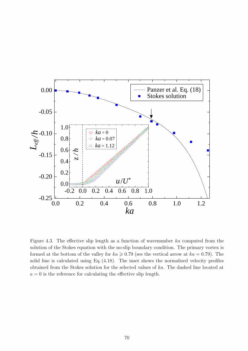
0.0 0.2 0.4 0.6 0.8 1.0 1.2-0.25

-0.20

-0.15

-0.10

-0.05

0.00

-0.2 0.0 0.2 0.4 0.6 0.8 1.00.0

0.2

0.4

0.6

0.8

1.0

Lef

f / h

Panzer et al. Eq. (18)Stokes solution

ka

ka = 1.12ka = 0.07ka = 0

. .

z / h

u /U*

Figure 4.3. The effective slip length as a function of wavenumber ka computed from the

solution of the Stokes equation with the no-slip boundary condition. The primary vortex is

formed at the bottom of the valley for ka > 0.79 (see the vertical arrow at ka = 0.79). The

solid line is calculated using Eq. (4.18). The inset shows the normalized velocity profiles

obtained from the Stokes solution for the selected values of ka. The dashed line located at

a = 0 is the reference for calculating the effective slip length.

70

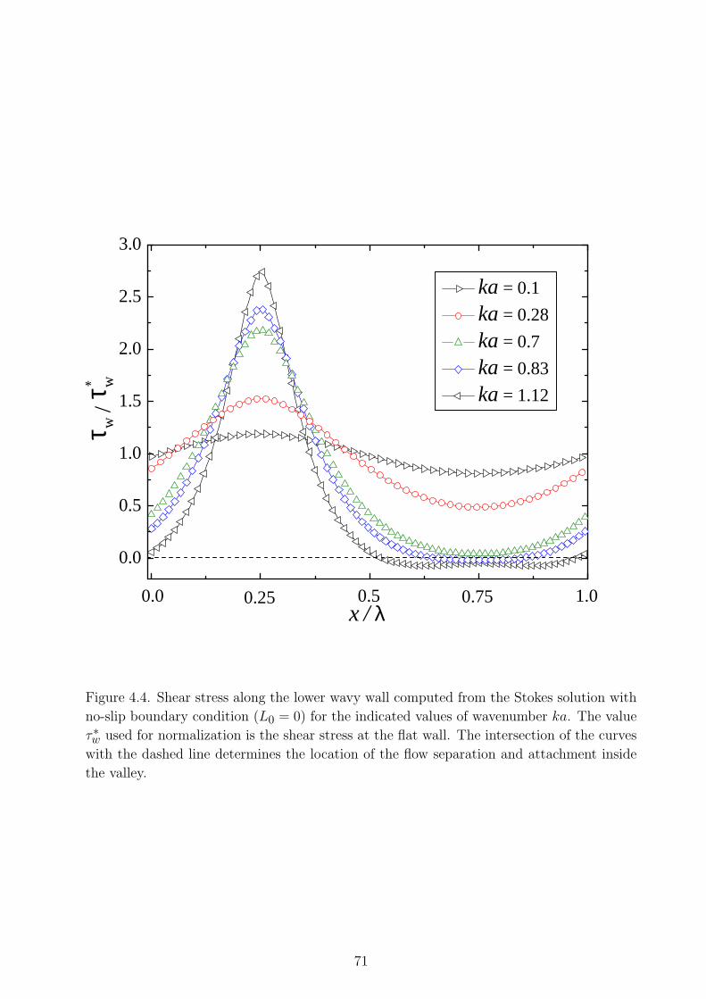
0.0

0.5

1.0

1.5

2.0

2.5

3.0

1.00.750.50.250.0x / λ

τ w

τ w/

*

ka = 0.1

ka = 0.28

ka = 0.7

ka = 0.83

ka = 1.12

Figure 4.4. Shear stress along the lower wavy wall computed from the Stokes solution with

no-slip boundary condition (L0 = 0) for the indicated values of wavenumber ka. The value

τ∗w used for normalization is the shear stress at the flat wall. The intersection of the curves

with the dashed line determines the location of the flow separation and attachment inside

the valley.

71

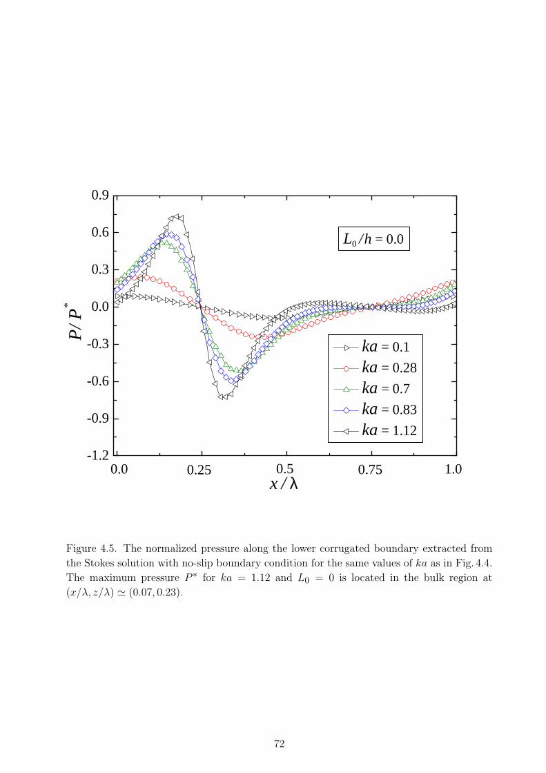
-1.2

-0.9

-0.6

-0.3

0.0

0.3

0.6

0.9

ka = 0.1

ka = 0.28

ka = 0.7

ka = 0.83

ka = 1.12

x / λ1.00.750.50.250.0

P/ P

*

L0 / h = 0.0

Figure 4.5. The normalized pressure along the lower corrugated boundary extracted from

the Stokes solution with no-slip boundary condition for the same values of ka as in Fig. 4.4.

The maximum pressure P ∗ for ka = 1.12 and L0 = 0 is located in the bulk region at

(x/λ, z/λ) ' (0.07, 0.23).

72

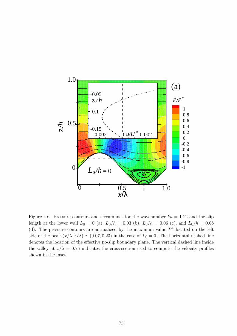
x

z

10.80.60.40.20

-0.2-0.4-0.6-0.8-1L0 = 0

/λ0 0.5 1.0

/h

0

0.5

1.0

P/P*

a( )

/h

-0.002 0 0.002-0.15

-0.1

-0.05

u/U *

z h/

Figure 4.6. Pressure contours and streamlines for the wavenumber ka = 1.12 and the slip

length at the lower wall L0 = 0 (a), L0/h = 0.03 (b), L0/h = 0.06 (c), and L0/h = 0.08

(d). The pressure contours are normalized by the maximum value P ∗ located on the left

side of the peak (x/λ, z/λ) ' (0.07, 0.23) in the case of L0 = 0. The horizontal dashed line

denotes the location of the effective no-slip boundary plane. The vertical dashed line inside

the valley at x/λ = 0.75 indicates the cross-section used to compute the velocity profiles

shown in the inset.

73

x

z

L /h0 = 0.03

/λ0 0.5 1.0

/h

0

0.5

1.0(b)

-0.002 0 0.002-0.15

-0.1

-0.05

u/U*

z h/

Figure 4.6. continued.

74

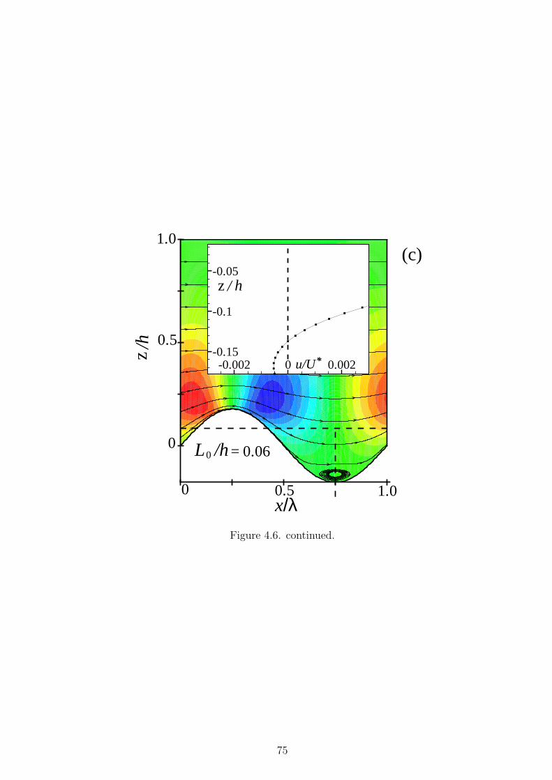
x

z

L /h0 = 0.06

/λ0 0.5 1.0

/h

0

0.5

1.0(c)

-0.002 0 0.002-0.15

-0.1

-0.05

u/U*

z h/

Figure 4.6. continued.

75

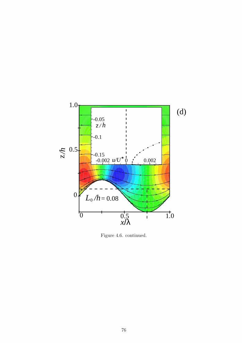
x

z

L /h0 = 0.08

/λ0 0.5 1.0

/h

0

0.5

1.0(d)

-0.002 0 0.002-0.15

-0.1

-0.05

u/U*

z h/

Figure 4.6. continued.

76

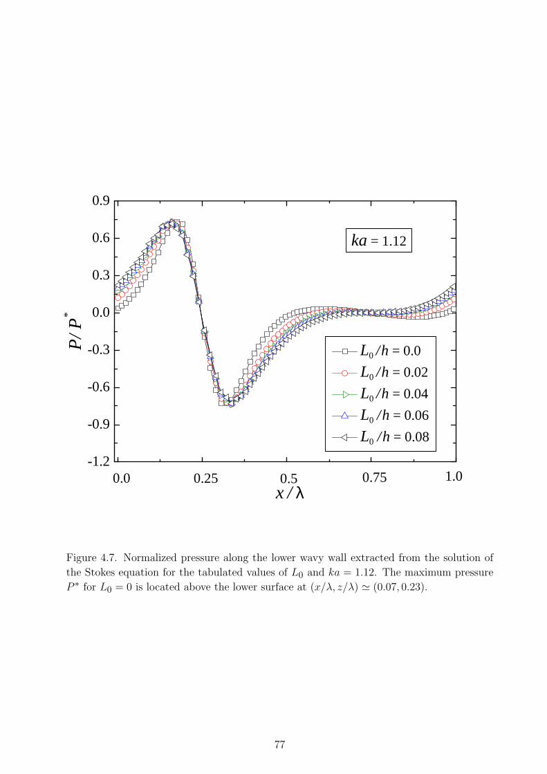
-1.2

-0.9

-0.6

-0.3

0.0

0.3

0.6

0.9

1.00.750.0 0.50.25x / λ

P/ P

*

L0 / h = 0.0

L0 / h = 0.02

L0 / h = 0.04

L0 / h = 0.06

L0 / h = 0.08

ka = 1.12

Figure 4.7. Normalized pressure along the lower wavy wall extracted from the solution of

the Stokes equation for the tabulated values of L0 and ka = 1.12. The maximum pressure

P ∗ for L0 = 0 is located above the lower surface at (x/λ, z/λ) ' (0.07, 0.23).

77

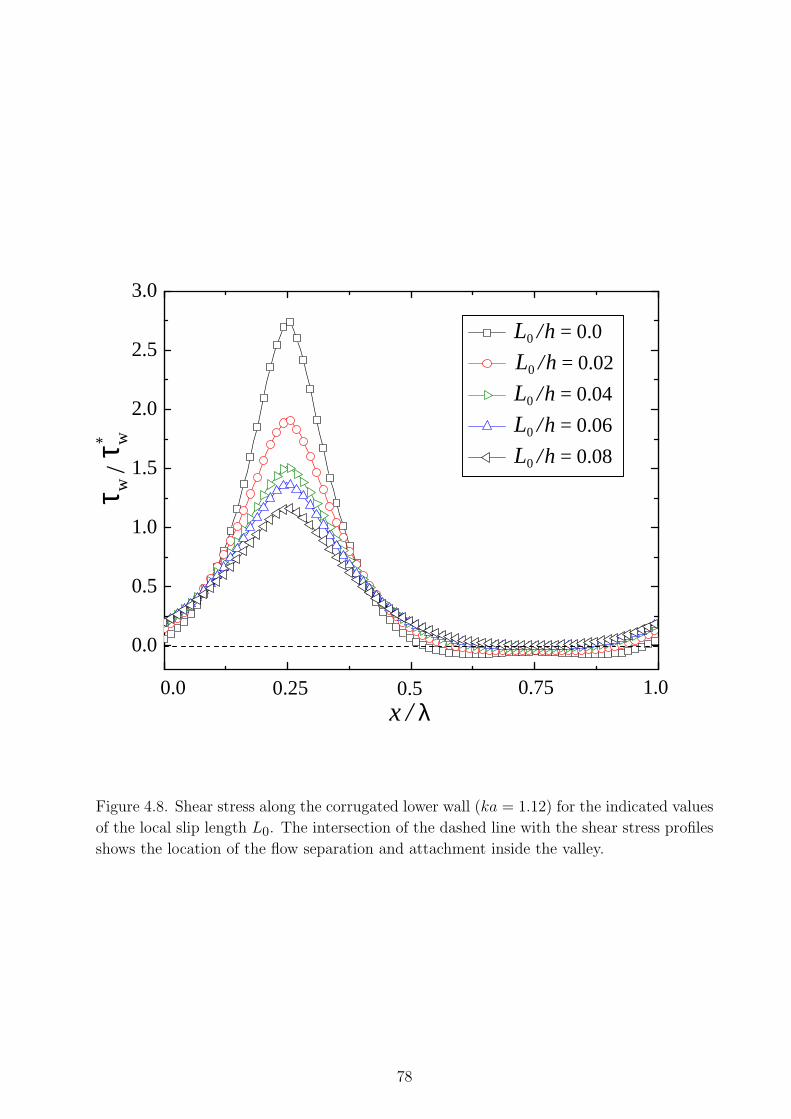
0.0

0.5

1.0

1.5

2.0

2.5

3.0

L0 / h = 0.0

L0 / h = 0.02

L0 / h = 0.04

L0 / h = 0.06

L0 / h = 0.08

1.00.750.50.250.0x / λ

τ w

τ w/

*

Figure 4.8. Shear stress along the corrugated lower wall (ka = 1.12) for the indicated values

of the local slip length L0. The intersection of the dashed line with the shear stress profiles

shows the location of the flow separation and attachment inside the valley.

78

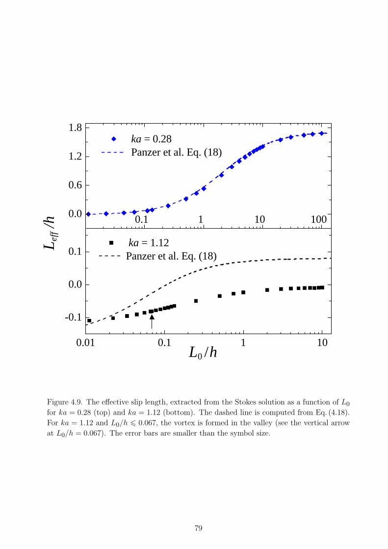
0.01 0.1 1 10

-0.1

0.0

0.1 ka = 1.12 Panzer et al. Eq. (18)

L

eff /

h

L0 / h

0.1 1 10 1000.0

0.6

1.2

1.8

ka = 0.28 Panzer et al. Eq. (18)

Figure 4.9. The effective slip length, extracted from the Stokes solution as a function of L0for ka = 0.28 (top) and ka = 1.12 (bottom). The dashed line is computed from Eq. (4.18).

For ka = 1.12 and L0/h 6 0.067, the vortex is formed in the valley (see the vertical arrow

at L0/h = 0.067). The error bars are smaller than the symbol size.

79

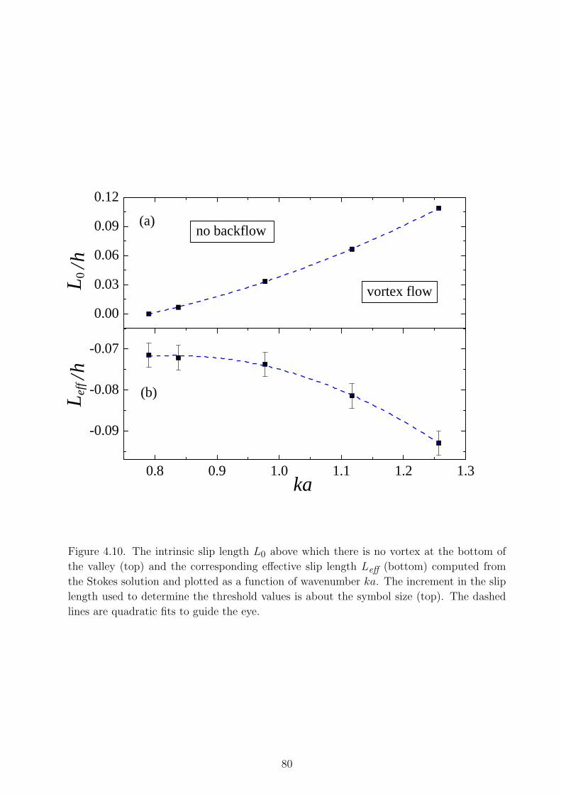
0.8 0.9 1.0 1.1 1.2 1.3

-0.09

-0.08

-0.07

(b)Lef

f / h

ka

0.00

0.03

0.06

0.09

0.12

(a)

vortex flowL0

/ h

no backflow

Figure 4.10. The intrinsic slip length L0 above which there is no vortex at the bottom of

the valley (top) and the corresponding effective slip length Leff (bottom) computed from

the Stokes solution and plotted as a function of wavenumber ka. The increment in the slip

length used to determine the threshold values is about the symbol size (top). The dashed

lines are quadratic fits to guide the eye.

80

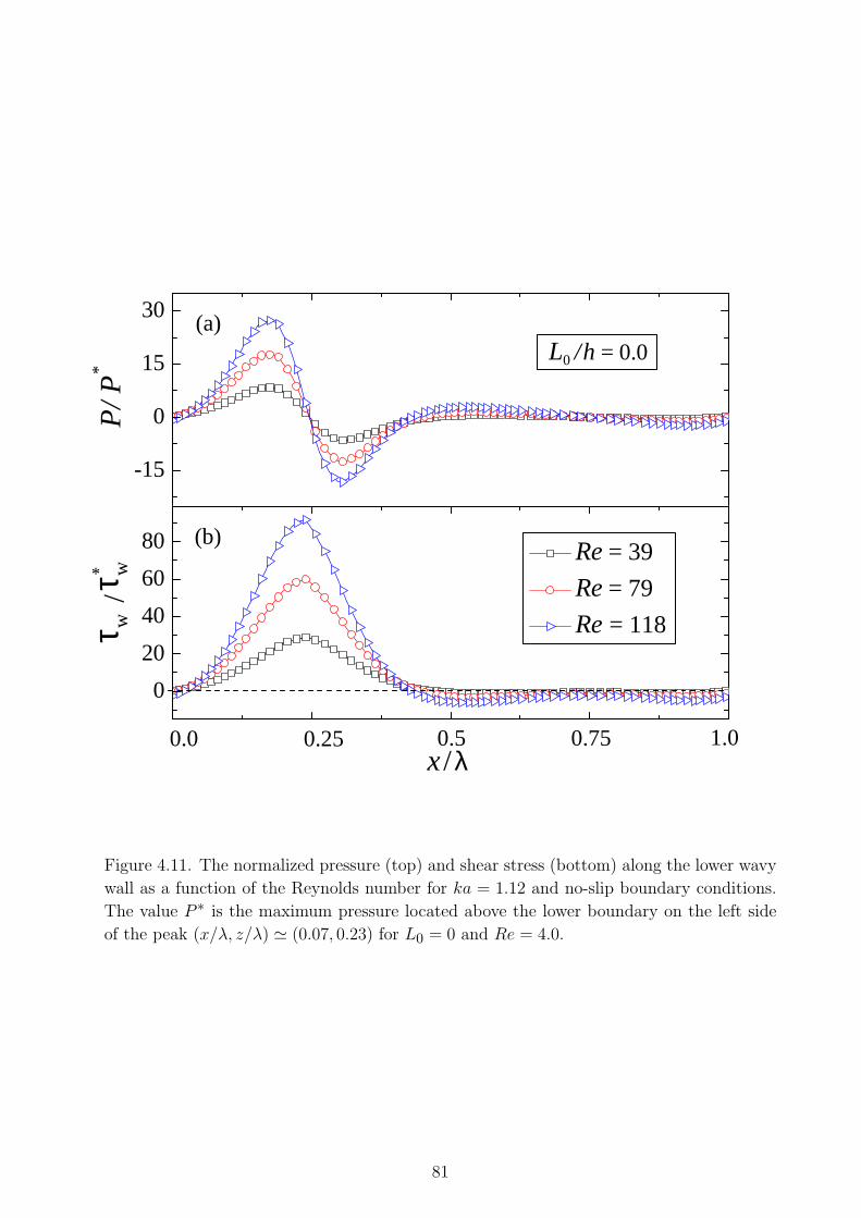
0

20

40

60

80 (b)

x / λ

τ w

τ w/

*

-15

0

15

30

P/ P

*

Re = 39

Re = 79

Re = 118

(a)L0 / h = 0.0

1.00.750.50.250.0

Figure 4.11. The normalized pressure (top) and shear stress (bottom) along the lower wavy

wall as a function of the Reynolds number for ka = 1.12 and no-slip boundary conditions.

The value P ∗ is the maximum pressure located above the lower boundary on the left side

of the peak (x/λ, z/λ) ' (0.07, 0.23) for L0 = 0 and Re = 4.0.

81

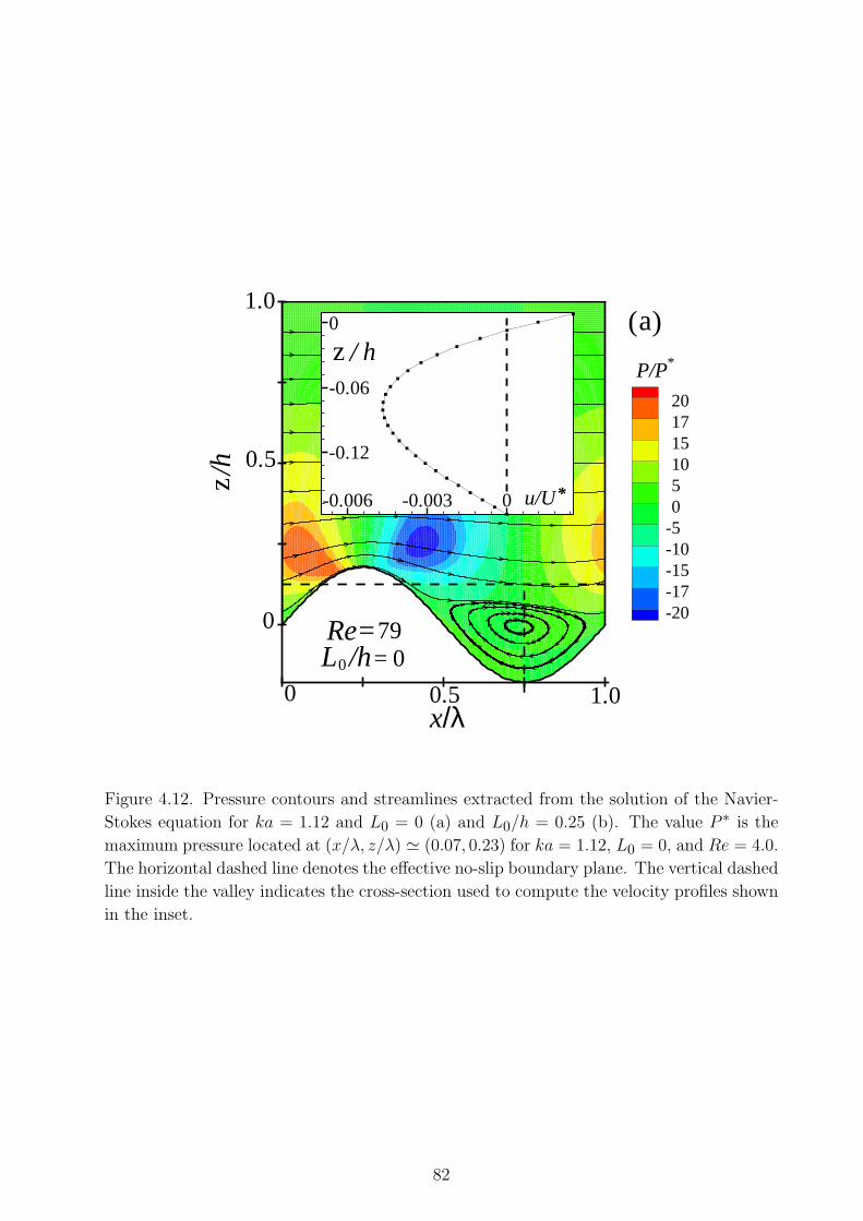
x

z

2017151050

-5-10-15-17-20

L0 = 0

/λ0 0.5 1.0

/h

0

0.5

1.0

Re=79

P/P*

/h

( )a

-0.006 -0.003 0

-0.12

-0.06

0

u/U*

z h/

Figure 4.12. Pressure contours and streamlines extracted from the solution of the Navier-

Stokes equation for ka = 1.12 and L0 = 0 (a) and L0/h = 0.25 (b). The value P ∗ is the

maximum pressure located at (x/λ, z/λ) ' (0.07, 0.23) for ka = 1.12, L0 = 0, and Re = 4.0.

The horizontal dashed line denotes the effective no-slip boundary plane. The vertical dashed

line inside the valley indicates the cross-section used to compute the velocity profiles shown

in the inset.

82

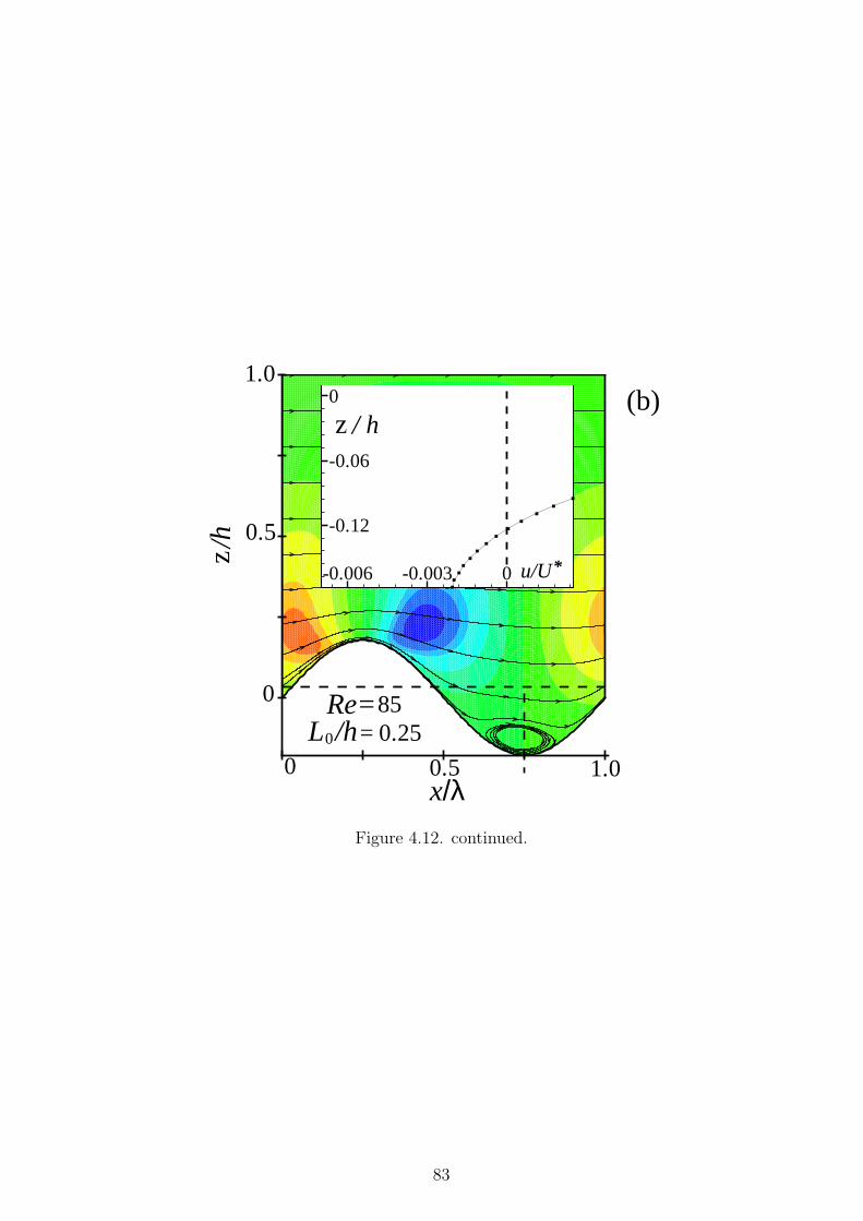
x

z

L0 = 0.25

/λ0 0.5 1.0

/h

0

0.5

1.0

Re=85/h

(b)

-0.006 -0.003 0

-0.12

-0.06

0

u/U*

z h/

Figure 4.12. continued.

83

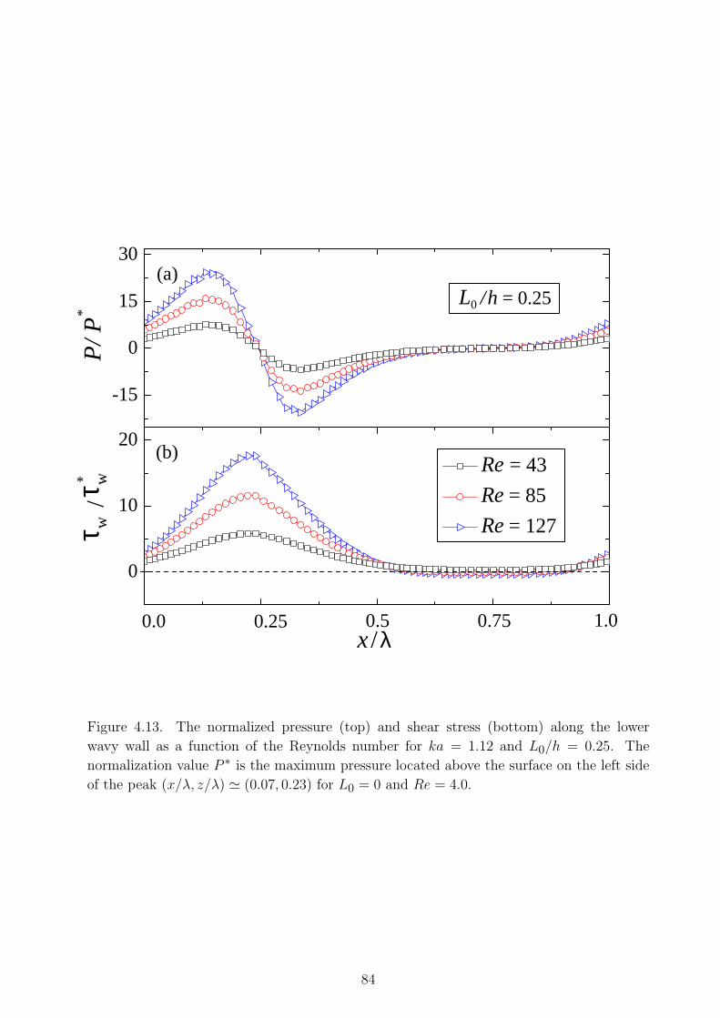
0

10

20(b)

x / λ

τ w

τ w/

*

-15

0

15

30

P/ P

*

Re = 43

Re = 85

Re = 127

(a)L0 / h = 0.25

1.00.750.50.250.0

Figure 4.13. The normalized pressure (top) and shear stress (bottom) along the lower

wavy wall as a function of the Reynolds number for ka = 1.12 and L0/h = 0.25. The

normalization value P ∗ is the maximum pressure located above the surface on the left side

of the peak (x/λ, z/λ) ' (0.07, 0.23) for L0 = 0 and Re = 4.0.

84

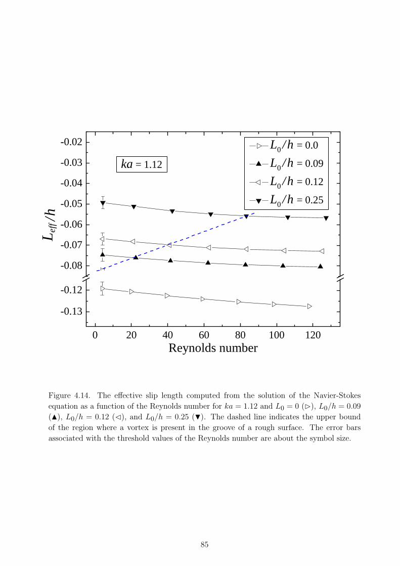
0 20 40 60 80 100 120

-0.13

-0.12

-0.08

-0.07

-0.06

-0.05

-0.04

-0.03

-0.02 L0 / h = 0.0

L0 / h = 0.09

L0 / h = 0.12

L0 / h = 0.25

Lef

f / h

Reynolds number

ka = 1.12

Figure 4.14. The effective slip length computed from the solution of the Navier-Stokes

equation as a function of the Reynolds number for ka = 1.12 and L0 = 0 (B), L0/h = 0.09

(N), L0/h = 0.12 (C), and L0/h = 0.25 (H). The dashed line indicates the upper bound

of the region where a vortex is present in the groove of a rough surface. The error bars

associated with the threshold values of the Reynolds number are about the symbol size.

85

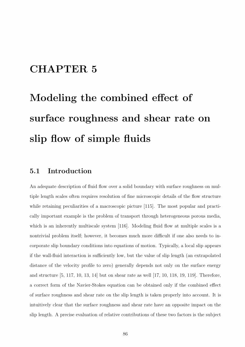
CHAPTER 5

Modeling the combined effect of

surface roughness and shear rate on

slip flow of simple fluids

5.1 Introduction

An adequate description of fluid flow over a solid boundary with surface roughness on mul-

tiple length scales often requires resolution of fine microscopic details of the flow structure

while retaining peculiarities of a macroscopic picture [115]. The most popular and practi-

cally important example is the problem of transport through heterogeneous porous media,

which is an inherently multiscale system [116]. Modeling fluid flow at multiple scales is a

nontrivial problem itself; however, it becomes much more difficult if one also needs to in-

corporate slip boundary conditions into equations of motion. Typically, a local slip appears

if the wall-fluid interaction is sufficiently low, but the value of slip length (an extrapolated

distance of the velocity profile to zero) generally depends not only on the surface energy

and structure [5, 117, 10, 13, 14] but on shear rate as well [17, 10, 118, 19, 119]. Therefore,

a correct form of the Navier-Stokes equation can be obtained only if the combined effect

of surface roughness and shear rate on the slip length is taken properly into account. It is

intuitively clear that the surface roughness and shear rate have an opposite impact on the

slip length. A precise evaluation of relative contributions of these two factors is the subject

86

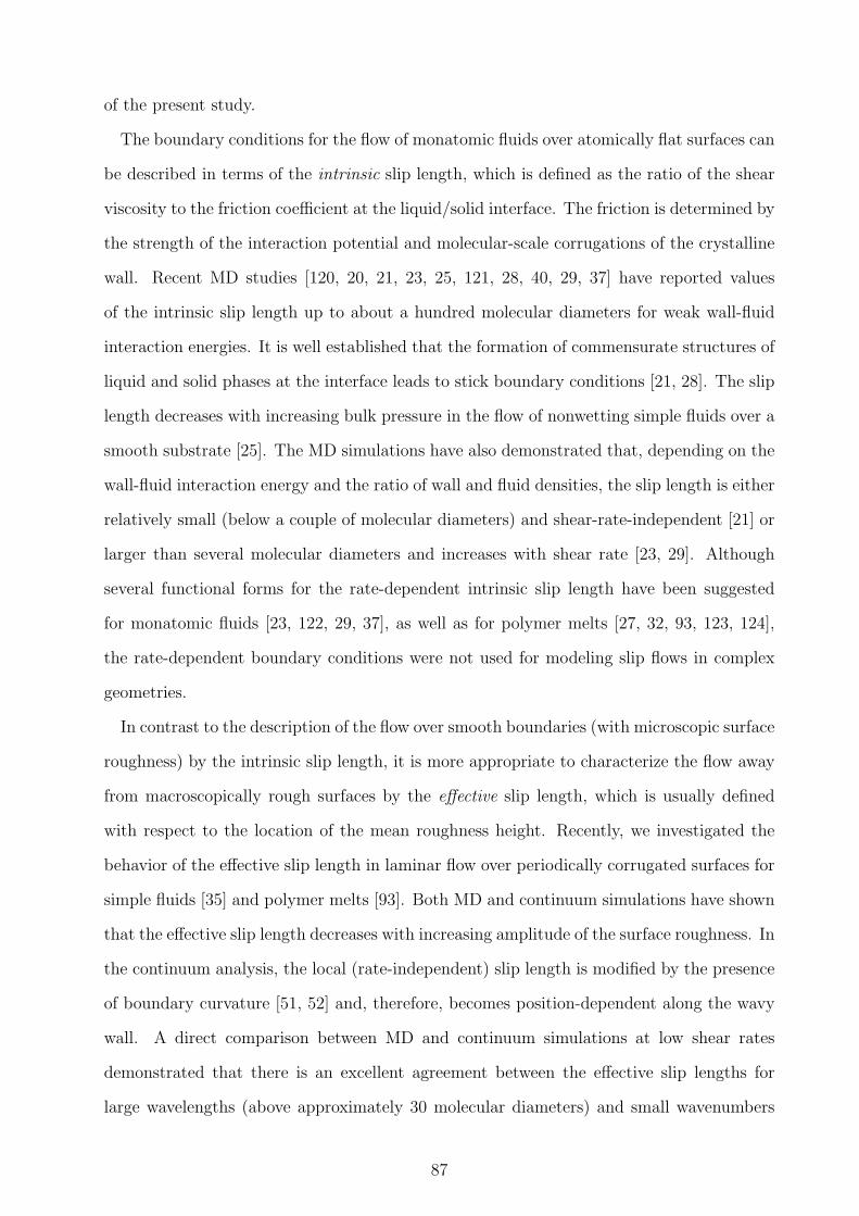
of the present study.

The boundary conditions for the flow of monatomic fluids over atomically flat surfaces can

be described in terms of the intrinsic slip length, which is defined as the ratio of the shear

viscosity to the friction coefficient at the liquid/solid interface. The friction is determined by

the strength of the interaction potential and molecular-scale corrugations of the crystalline

wall. Recent MD studies [120, 20, 21, 23, 25, 121, 28, 40, 29, 37] have reported values

of the intrinsic slip length up to about a hundred molecular diameters for weak wall-fluid

interaction energies. It is well established that the formation of commensurate structures of

liquid and solid phases at the interface leads to stick boundary conditions [21, 28]. The slip

length decreases with increasing bulk pressure in the flow of nonwetting simple fluids over a

smooth substrate [25]. The MD simulations have also demonstrated that, depending on the

wall-fluid interaction energy and the ratio of wall and fluid densities, the slip length is either

relatively small (below a couple of molecular diameters) and shear-rate-independent [21] or

larger than several molecular diameters and increases with shear rate [23, 29]. Although

several functional forms for the rate-dependent intrinsic slip length have been suggested

for monatomic fluids [23, 122, 29, 37], as well as for polymer melts [27, 32, 93, 123, 124],

the rate-dependent boundary conditions were not used for modeling slip flows in complex

geometries.

In contrast to the description of the flow over smooth boundaries (with microscopic surface

roughness) by the intrinsic slip length, it is more appropriate to characterize the flow away

from macroscopically rough surfaces by the effective slip length, which is usually defined

with respect to the location of the mean roughness height. Recently, we investigated the

behavior of the effective slip length in laminar flow over periodically corrugated surfaces for

simple fluids [35] and polymer melts [93]. Both MD and continuum simulations have shown

that the effective slip length decreases with increasing amplitude of the surface roughness. In

the continuum analysis, the local (rate-independent) slip length is modified by the presence

of boundary curvature [51, 52] and, therefore, becomes position-dependent along the wavy

wall. A direct comparison between MD and continuum simulations at low shear rates

demonstrated that there is an excellent agreement between the effective slip lengths for

large wavelengths (above approximately 30 molecular diameters) and small wavenumbers

87

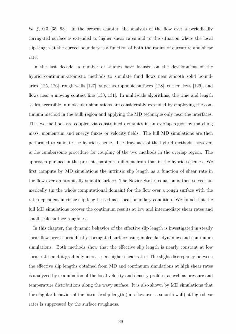
ka . 0.3 [35, 93]. In the present chapter, the analysis of the flow over a periodically

corrugated surface is extended to higher shear rates and to the situation where the local

slip length at the curved boundary is a function of both the radius of curvature and shear

rate.

In the last decade, a number of studies have focused on the development of the

hybrid continuum-atomistic methods to simulate fluid flows near smooth solid bound-

aries [125, 126], rough walls [127], superhydrophobic surfaces [128], corner flows [129], and

flows near a moving contact line [130, 131]. In multiscale algorithms, the time and length

scales accessible in molecular simulations are considerably extended by employing the con-

tinuum method in the bulk region and applying the MD technique only near the interfaces.

The two methods are coupled via constrained dynamics in an overlap region by matching

mass, momentum and energy fluxes or velocity fields. The full MD simulations are then

performed to validate the hybrid scheme. The drawback of the hybrid methods, however,

is the cumbersome procedure for coupling of the two methods in the overlap region. The

approach pursued in the present chapter is different from that in the hybrid schemes. We

first compute by MD simulations the intrinsic slip length as a function of shear rate in

the flow over an atomically smooth surface. The Navier-Stokes equation is then solved nu-

merically (in the whole computational domain) for the flow over a rough surface with the

rate-dependent intrinsic slip length used as a local boundary condition. We found that the

full MD simulations recover the continuum results at low and intermediate shear rates and

small-scale surface roughness.

In this chapter, the dynamic behavior of the effective slip length is investigated in steady

shear flow over a periodically corrugated surface using molecular dynamics and continuum

simulations. Both methods show that the effective slip length is nearly constant at low

shear rates and it gradually increases at higher shear rates. The slight discrepancy between

the effective slip lengths obtained from MD and continuum simulations at high shear rates

is analyzed by examination of the local velocity and density profiles, as well as pressure and

temperature distributions along the wavy surface. It is also shown by MD simulations that

the singular behavior of the intrinsic slip length (in a flow over a smooth wall) at high shear

rates is suppressed by the surface roughness.

88

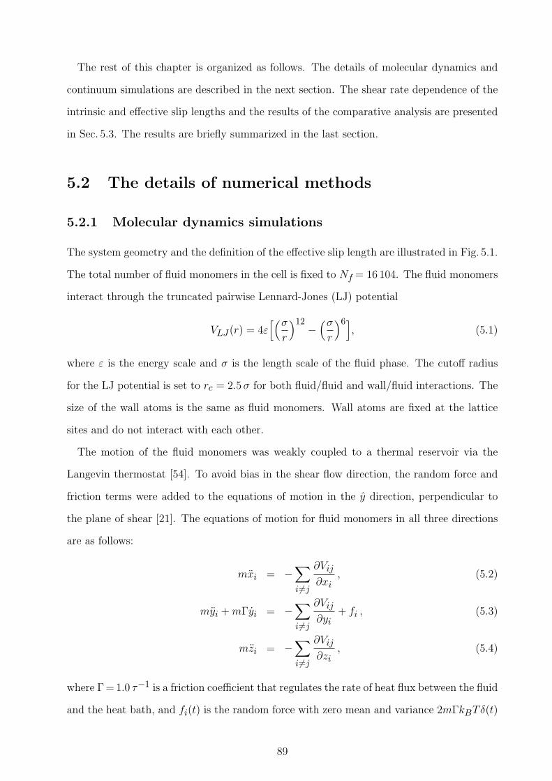
The rest of this chapter is organized as follows. The details of molecular dynamics and

continuum simulations are described in the next section. The shear rate dependence of the

intrinsic and effective slip lengths and the results of the comparative analysis are presented

in Sec. 5.3. The results are briefly summarized in the last section.

5.2 The details of numerical methods

5.2.1 Molecular dynamics simulations

The system geometry and the definition of the effective slip length are illustrated in Fig. 5.1.

The total number of fluid monomers in the cell is fixed to Nf = 16 104. The fluid monomers

interact through the truncated pairwise Lennard-Jones (LJ) potential

VLJ (r) = 4ε[(σ

r

)12 −(σ

r

)6], (5.1)

where ε is the energy scale and σ is the length scale of the fluid phase. The cutoff radius

for the LJ potential is set to rc = 2.5 σ for both fluid/fluid and wall/fluid interactions. The

size of the wall atoms is the same as fluid monomers. Wall atoms are fixed at the lattice

sites and do not interact with each other.

The motion of the fluid monomers was weakly coupled to a thermal reservoir via the

Langevin thermostat [54]. To avoid bias in the shear flow direction, the random force and

friction terms were added to the equations of motion in the y direction, perpendicular to

the plane of shear [21]. The equations of motion for fluid monomers in all three directions

are as follows:

mxi = −∑

i6=j

∂Vij

∂xi, (5.2)

myi + mΓyi = −∑

i6=j

∂Vij

∂yi+ fi , (5.3)

mzi = −∑

i6=j

∂Vij

∂zi, (5.4)

where Γ = 1.0 τ−1 is a friction coefficient that regulates the rate of heat flux between the fluid

and the heat bath, and fi(t) is the random force with zero mean and variance 2mΓkBTδ(t)

89

determined from the fluctuation-dissipation relation. Unless otherwise specified, the tem-

perature of the Langevin thermostat is set to T = 1.1 ε/kB , where kB is the Boltzmann

constant. The equations of motion were integrated using the Verlet algorithm [56] with a

time step ∆t = 0.002 τ , where τ =√

mσ2/ε is the characteristic time of the LJ potential.

The intrinsic slip length was computed at the lower flat wall composed out of two layers

of the FCC lattice with density ρw = 3.1 σ−3 and nearest-neighbor distance d = 0.77 σ be-

tween atoms in the xy plane. The partial slip is permitted along the lower boundary due

to relatively low wall-fluid interaction energy εwf = 0.5 ε. The no-slip boundary condition

is enforced at the flat upper wall with a lower density 0.67 σ−3 by allowing the formation of

commensurate structures of liquid and solid phases at the interface. The nearest-neighbor

distance between wall atoms is 1.28 σ in the (111) plane of the FCC lattice. The wall-fluid

interaction energy ε ensures the no-slip condition at the upper wall holds even at high shear

rates. The cell dimensions are set to Lx = 42.34 σ and Ly = 10.0 σ parallel to the confining

walls. The MD simulations were performed at a constant fluid density (ρ = 0.81 σ−3) en-

semble, i.e., the relative distance between the walls was always fixed to Lz = 41.41 σ in the

z direction. Periodic boundary conditions were applied along the x and y directions.

The effect of surface roughness on slip flow was investigated in the cell with a lower

sinusoidal wall with wavelength λ = Lx and amplitude a = 1.82 σ (see Fig. 5.1). Special

care was taken to make the lower corrugated wall with a uniform density ρw = 3.1 σ−3 (by

including additional rows of atoms along the y direction) so that the lattice spacing along

the sinusoidal curve remained d = 0.77 σ.

The fluid monomer velocities were initialized using the Maxwell-Boltzmann probability

distribution at the temperature T = 1.1 ε/kB . After an equilibration period of about 2 ×104 τ , the velocity and density profiles across the channel were averaged for about 2× 105 τ

within bins of Lx × Ly × ∆z, where ∆z = 0.01 σ. The location and dimensions of the

averaging regions for the computation of the local velocity and density profiles will be

specified in Sec. 5.3.3.

90

5.2.2 Continuum simulations

The two-dimensional, steady-state and incompressible Navier-Stokes (NS) equation is solved

numerically using the finite element method. The equation of motion based on these as-

sumptions is written as follows:

ρu · ∇u = −∇p + µ∇2u, (5.5)

where u = u i + vj is the velocity vector, ρ is the density of the fluid, and p and µ are the

pressure field and fluid viscosity, respectively.

The penalty formulation was implemented for the incompressible solution to avoid de-

coupling of the velocity and pressure terms [57]. In the penalty formulation, the continuity

equation, ∇ · u = 0, is replaced with a perturbed equation

∇ · u = − p

Λ, (5.6)

where Λ is the penalty parameter, which enforces the incompressibility condition. For most

practical situations, where computation is performed with double-precision 64 bit words,

a penalty parameter (Λ) between 107 and 109 is sufficient to conserve the accuracy [57].

After substitution of the pressure term in Eq. (5.6) into Eq. (5.5), the modified momentum

equation can be rewritten as follows:

ρu · ∇u = Λ∇(∇ · u) + µ∇2u. (5.7)

The Galerkin method with rectangular bilinear isoparametric elements is used to integrate

the Navier-Stokes equation [57, 132].

The boundary conditions are applied at the inlet, outlet, and upper and lower walls.

The periodic boundary conditions are implemented along the x direction for the inlet and

outlet. The boundary condition at the upper wall is always no-slip. A partial slip boundary

condition is applied at the lower wall. In addition to the global coordinate system (x, z), a

local coordinate system (~t, ~n) is defined along the lower curved boundary with unit vectors

~t and ~n representing the tangential and normal directions, respectively. The tangential

component of the fluid velocity in the local coordinate system can be computed as

ut = L0[(~n · ∇) ut + ut/R], (5.8)

91

where R is the local radius of curvature and L0 is the intrinsic slip length at the flat

liquid/solid interface [52]. The radius of curvature R is positive and negative for concave

and convex regions, respectively. The second-order forward-differencing scheme was used to

compute accurately the normal derivative of the tangential velocity (~n · ∇) ut at the lower

boundary.

At the beginning of the simulation procedure, the boundary conditions at the upper and

lower walls are set to no-slip. Then, the equations of motion are solved implicitly and the

tangential velocities at the lower boundary are updated according to Eq. (5.8). In the next

step, the updated velocities at the lower boundary are used as a new boundary condition and

the equations of motion are solved again. The iterative process is repeated until a desired

accuracy is achieved. The convergence rate of the solution was controlled by applying an

under-relaxation factor of 0.001 for the boundary nodes. For all results reported in the

present chapter, the continuum simulations were performed with 150× 150 grid resolution.

However, the accuracy of the results was also checked by performing a set of simulations

using a finer grid 180× 180. The maximum error in the effective slip length due to the grid

resolution is Leff/Lz = 0.003. The same error bars were reported in the previous study of

laminar flow over a periodically corrugated surface with either no-slip or (rate-independent)

slip boundary conditions [132].

The averaged error of the solution is defined as

error =[ Np∑

i=1

| uni − un+1

i || un+1

i |]/Np, (5.9)

where Np is the number of nodes in the computational domain, uni is the magnitude of

the velocity at node i and time step n, and un+1i is the magnitude of the velocity in

the next time step. The solution is converged when error 6 10−9 and the tangential

velocities along the lower boundary satisfy ut = Llocal∂ut∂n , where the local slip length is

Llocal = (L−10 −R−1)−1 [52].

92

5.3 Results

5.3.1 MD simulations: the intrinsic and effective slip lengths

We first consider flow in the cell with flat upper and lower walls. The averaged velocity

profiles are plotted in Fig. 5.2 for the selected upper wall speeds. The profiles are linear

throughout the channel except for a slight curvature near the lower wall at U = 5.0 σ/τ .

Note that with increasing upper wall speed, the slip velocity at the lower wall increases

monotonically up to about 2 σ/τ at U = 5.0 σ/τ . The flow velocity at the top boundary

remains equal to the upper wall speed due to the commensurability of liquid and solid

structures at the interface and sufficiently high wall-fluid interaction energy. The shear rate

was estimated from the linear slope of the velocity profiles across the entire cell.

The fluid viscosity computed from the Kirkwood relation [58] is plotted in Fig. 5.3 as a

function of shear rate in the cell with flat walls. In agreement with the results of previous MD

studies on shear flow of simple fluids [23, 29, 37], the shear viscosity µ = 2.15± 0.15 ετσ−3

remains rate-independent up to γτ ' 0.072, which corresponds to the upper wall speed

U = 5.375 σ/τ . It is also known that at high shear rates the fluid temperature profiles become

nonuniform across the cell and the heating up is larger near the interfaces [29, 37, 32]. To

ensure that the fluid viscosity is not affected by the heating up, we performed two additional

sets of simulations at the upper wall speeds U = 1.0 σ/τ and U = 3.5 σ/τ and increased the

temperature of the Langevin thermostat with an increment of 0.05 ε/kB . In the range

of the thermostat temperatures and error bars reported in Fig. 5.3, the shear viscosity

is independent of temperature for both upper wall speeds. In Sec. 5.3.3, the results of

simulations performed at higher temperatures will be used to estimate the effect of pressure

on the slip length.

The intrinsic slip length L0 in the flow over a flat lower wall was determined from the

linear extrapolation of velocity profiles to zero with respect to the reference plane located

0.5 σ above the FCC lattice plane. The variation of the intrinsic slip length as a function

of shear rate is presented in Fig. 5.4. At low shear rates γτ . 0.005, the slip length is nearly

constant. The leftmost data point reported in Fig. 5.4 is γτ ' 1.7× 10−4 at the upper wall

speed U = 0.01 σ/τ . At higher shear rates, the intrinsic slip length first gradually increases

93

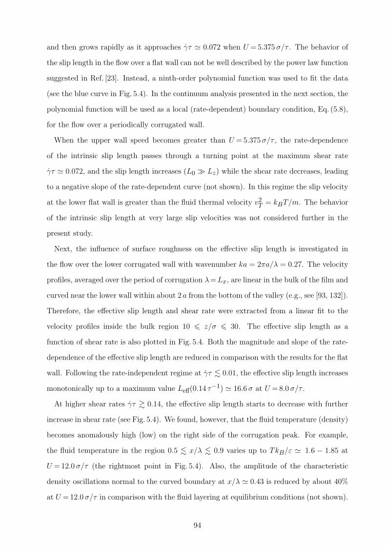
and then grows rapidly as it approaches γτ ' 0.072 when U = 5.375 σ/τ . The behavior of

the slip length in the flow over a flat wall can not be well described by the power law function

suggested in Ref. [23]. Instead, a ninth-order polynomial function was used to fit the data

(see the blue curve in Fig. 5.4). In the continuum analysis presented in the next section, the

polynomial function will be used as a local (rate-dependent) boundary condition, Eq. (5.8),

for the flow over a periodically corrugated wall.

When the upper wall speed becomes greater than U = 5.375 σ/τ , the rate-dependence

of the intrinsic slip length passes through a turning point at the maximum shear rate

γτ ' 0.072, and the slip length increases (L0 À Lz) while the shear rate decreases, leading

to a negative slope of the rate-dependent curve (not shown). In this regime the slip velocity

at the lower flat wall is greater than the fluid thermal velocity v2T = kBT/m. The behavior

of the intrinsic slip length at very large slip velocities was not considered further in the

present study.

Next, the influence of surface roughness on the effective slip length is investigated in

the flow over the lower corrugated wall with wavenumber ka = 2πa/λ = 0.27. The velocity

profiles, averaged over the period of corrugation λ = Lx, are linear in the bulk of the film and

curved near the lower wall within about 2 a from the bottom of the valley (e.g., see [93, 132]).

Therefore, the effective slip length and shear rate were extracted from a linear fit to the

velocity profiles inside the bulk region 10 6 z/σ 6 30. The effective slip length as a

function of shear rate is also plotted in Fig. 5.4. Both the magnitude and slope of the rate-

dependence of the effective slip length are reduced in comparison with the results for the flat

wall. Following the rate-independent regime at γτ . 0.01, the effective slip length increases

monotonically up to a maximum value Leff(0.14 τ−1) ' 16.6 σ at U = 8.0 σ/τ .

At higher shear rates γτ & 0.14, the effective slip length starts to decrease with further

increase in shear rate (see Fig. 5.4). We found, however, that the fluid temperature (density)

becomes anomalously high (low) on the right side of the corrugation peak. For example,

the fluid temperature in the region 0.5 . x/λ . 0.9 varies up to TkB/ε ' 1.6 − 1.85 at

U = 12.0 σ/τ (the rightmost point in Fig. 5.4). Also, the amplitude of the characteristic

density oscillations normal to the curved boundary at x/λ ' 0.43 is reduced by about 40%

at U = 12.0 σ/τ in comparison with the fluid layering at equilibrium conditions (not shown).

94

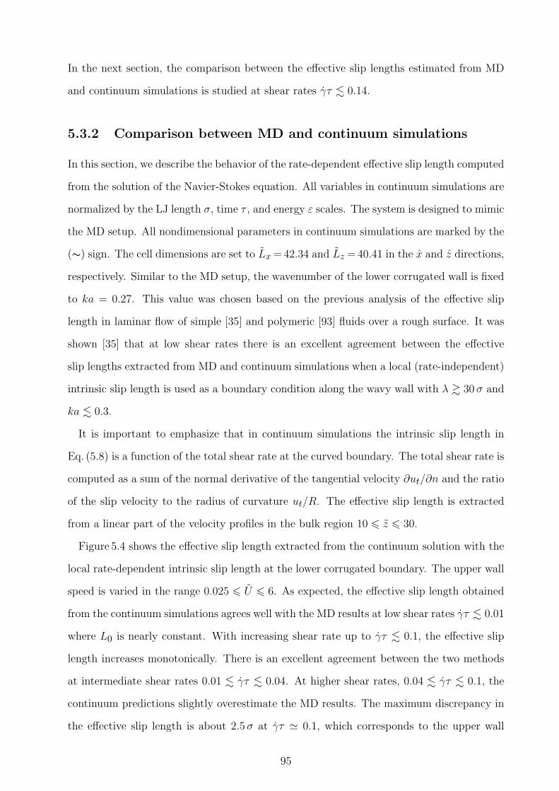
In the next section, the comparison between the effective slip lengths estimated from MD

and continuum simulations is studied at shear rates γτ . 0.14.

5.3.2 Comparison between MD and continuum simulations

In this section, we describe the behavior of the rate-dependent effective slip length computed

from the solution of the Navier-Stokes equation. All variables in continuum simulations are

normalized by the LJ length σ, time τ , and energy ε scales. The system is designed to mimic

the MD setup. All nondimensional parameters in continuum simulations are marked by the

(∼) sign. The cell dimensions are set to Lx = 42.34 and Lz = 40.41 in the x and z directions,

respectively. Similar to the MD setup, the wavenumber of the lower corrugated wall is fixed

to ka = 0.27. This value was chosen based on the previous analysis of the effective slip

length in laminar flow of simple [35] and polymeric [93] fluids over a rough surface. It was

shown [35] that at low shear rates there is an excellent agreement between the effective

slip lengths extracted from MD and continuum simulations when a local (rate-independent)

intrinsic slip length is used as a boundary condition along the wavy wall with λ & 30 σ and

ka . 0.3.

It is important to emphasize that in continuum simulations the intrinsic slip length in

Eq. (5.8) is a function of the total shear rate at the curved boundary. The total shear rate is

computed as a sum of the normal derivative of the tangential velocity ∂ut/∂n and the ratio

of the slip velocity to the radius of curvature ut/R. The effective slip length is extracted

from a linear part of the velocity profiles in the bulk region 10 6 z 6 30.

Figure 5.4 shows the effective slip length extracted from the continuum solution with the

local rate-dependent intrinsic slip length at the lower corrugated boundary. The upper wall

speed is varied in the range 0.025 6 U 6 6. As expected, the effective slip length obtained

from the continuum simulations agrees well with the MD results at low shear rates γτ . 0.01

where L0 is nearly constant. With increasing shear rate up to γτ . 0.1, the effective slip

length increases monotonically. There is an excellent agreement between the two methods

at intermediate shear rates 0.01 . γτ . 0.04. At higher shear rates, 0.04 . γτ . 0.1, the

continuum predictions slightly overestimate the MD results. The maximum discrepancy in

the effective slip length is about 2.5 σ at γτ ' 0.1, which corresponds to the upper wall

95

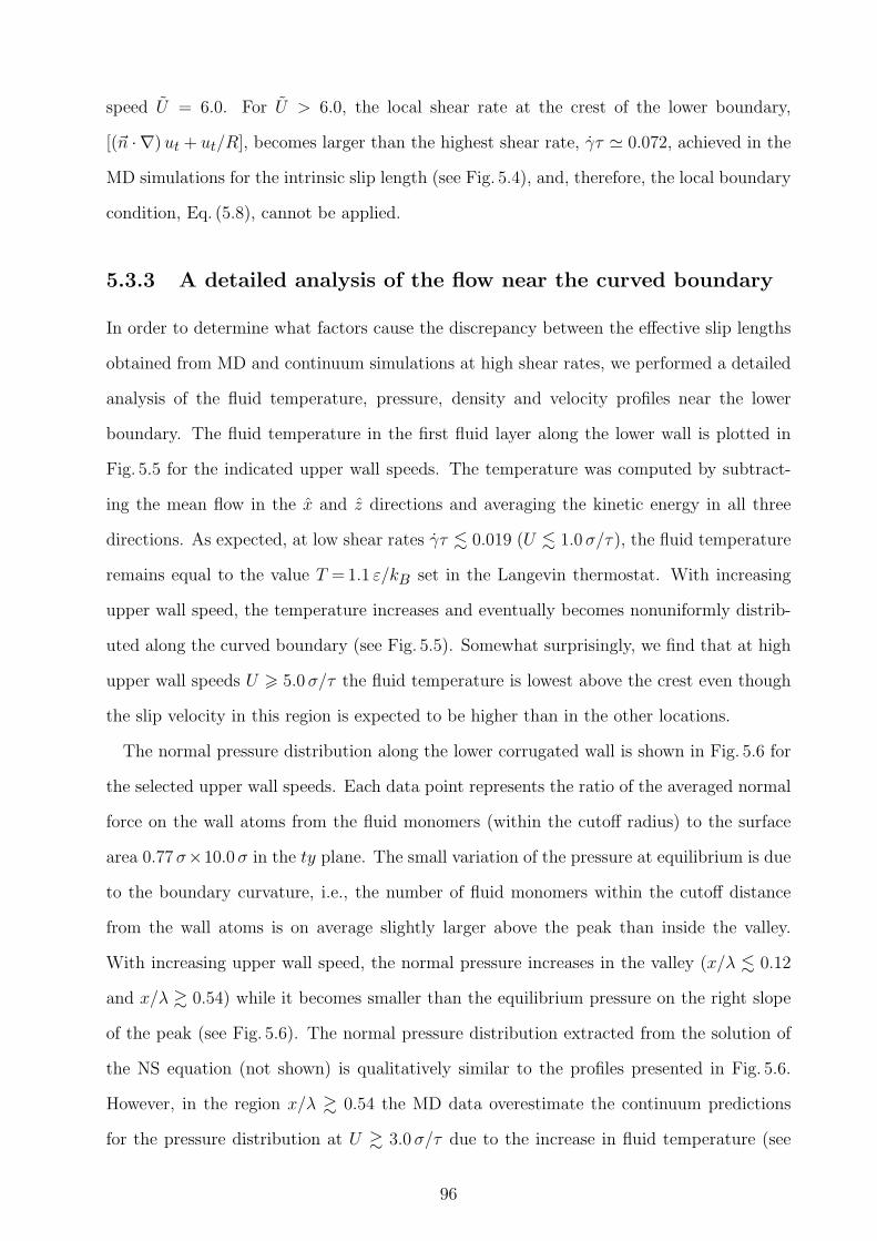
speed U = 6.0. For U > 6.0, the local shear rate at the crest of the lower boundary,

[(~n · ∇) ut + ut/R], becomes larger than the highest shear rate, γτ ' 0.072, achieved in the

MD simulations for the intrinsic slip length (see Fig. 5.4), and, therefore, the local boundary

condition, Eq. (5.8), cannot be applied.

5.3.3 A detailed analysis of the flow near the curved boundary

In order to determine what factors cause the discrepancy between the effective slip lengths

obtained from MD and continuum simulations at high shear rates, we performed a detailed

analysis of the fluid temperature, pressure, density and velocity profiles near the lower

boundary. The fluid temperature in the first fluid layer along the lower wall is plotted in

Fig. 5.5 for the indicated upper wall speeds. The temperature was computed by subtract-

ing the mean flow in the x and z directions and averaging the kinetic energy in all three

directions. As expected, at low shear rates γτ . 0.019 (U . 1.0 σ/τ), the fluid temperature

remains equal to the value T = 1.1 ε/kB set in the Langevin thermostat. With increasing

upper wall speed, the temperature increases and eventually becomes nonuniformly distrib-

uted along the curved boundary (see Fig. 5.5). Somewhat surprisingly, we find that at high

upper wall speeds U > 5.0 σ/τ the fluid temperature is lowest above the crest even though

the slip velocity in this region is expected to be higher than in the other locations.

The normal pressure distribution along the lower corrugated wall is shown in Fig. 5.6 for

the selected upper wall speeds. Each data point represents the ratio of the averaged normal

force on the wall atoms from the fluid monomers (within the cutoff radius) to the surface

area 0.77 σ×10.0 σ in the ty plane. The small variation of the pressure at equilibrium is due

to the boundary curvature, i.e., the number of fluid monomers within the cutoff distance

from the wall atoms is on average slightly larger above the peak than inside the valley.

With increasing upper wall speed, the normal pressure increases in the valley (x/λ . 0.12

and x/λ & 0.54) while it becomes smaller than the equilibrium pressure on the right slope

of the peak (see Fig. 5.6). The normal pressure distribution extracted from the solution of

the NS equation (not shown) is qualitatively similar to the profiles presented in Fig. 5.6.

However, in the region x/λ & 0.54 the MD data overestimate the continuum predictions

for the pressure distribution at U & 3.0 σ/τ due to the increase in fluid temperature (see

96

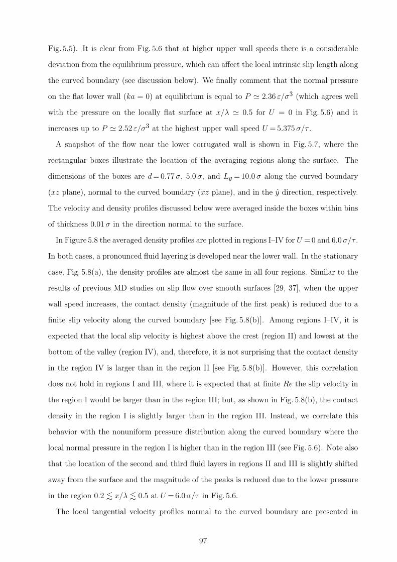
Fig. 5.5). It is clear from Fig. 5.6 that at higher upper wall speeds there is a considerable

deviation from the equilibrium pressure, which can affect the local intrinsic slip length along

the curved boundary (see discussion below). We finally comment that the normal pressure

on the flat lower wall (ka = 0) at equilibrium is equal to P ' 2.36 ε/σ3 (which agrees well

with the pressure on the locally flat surface at x/λ ' 0.5 for U = 0 in Fig. 5.6) and it

increases up to P ' 2.52 ε/σ3 at the highest upper wall speed U = 5.375 σ/τ .

A snapshot of the flow near the lower corrugated wall is shown in Fig. 5.7, where the

rectangular boxes illustrate the location of the averaging regions along the surface. The

dimensions of the boxes are d = 0.77 σ, 5.0 σ, and Ly = 10.0 σ along the curved boundary

(xz plane), normal to the curved boundary (xz plane), and in the y direction, respectively.

The velocity and density profiles discussed below were averaged inside the boxes within bins

of thickness 0.01 σ in the direction normal to the surface.

In Figure 5.8 the averaged density profiles are plotted in regions I–IV for U = 0 and 6.0 σ/τ .

In both cases, a pronounced fluid layering is developed near the lower wall. In the stationary

case, Fig. 5.8(a), the density profiles are almost the same in all four regions. Similar to the

results of previous MD studies on slip flow over smooth surfaces [29, 37], when the upper

wall speed increases, the contact density (magnitude of the first peak) is reduced due to a

finite slip velocity along the curved boundary [see Fig. 5.8(b)]. Among regions I–IV, it is

expected that the local slip velocity is highest above the crest (region II) and lowest at the

bottom of the valley (region IV), and, therefore, it is not surprising that the contact density

in the region IV is larger than in the region II [see Fig. 5.8(b)]. However, this correlation

does not hold in regions I and III, where it is expected that at finite Re the slip velocity in

the region I would be larger than in the region III; but, as shown in Fig. 5.8(b), the contact

density in the region I is slightly larger than in the region III. Instead, we correlate this

behavior with the nonuniform pressure distribution along the curved boundary where the

local normal pressure in the region I is higher than in the region III (see Fig. 5.6). Note also

that the location of the second and third fluid layers in regions II and III is slightly shifted

away from the surface and the magnitude of the peaks is reduced due to the lower pressure

in the region 0.2 . x/λ . 0.5 at U = 6.0 σ/τ in Fig. 5.6.

The local tangential velocity profiles normal to the curved boundary are presented in

97

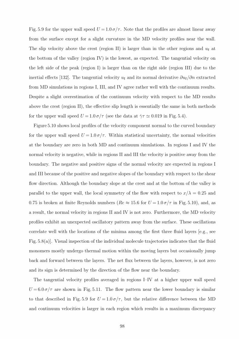
Fig. 5.9 for the upper wall speed U = 1.0 σ/τ . Note that the profiles are almost linear away

from the surface except for a slight curvature in the MD velocity profiles near the wall.

The slip velocity above the crest (region II) is larger than in the other regions and ut at

the bottom of the valley (region IV) is the lowest, as expected. The tangential velocity on

the left side of the peak (region I) is larger than on the right side (region III) due to the

inertial effects [132]. The tangential velocity ut and its normal derivative ∂ut/∂n extracted

from MD simulations in regions I, III, and IV agree rather well with the continuum results.

Despite a slight overestimation of the continuum velocity with respect to the MD results

above the crest (region II), the effective slip length is essentially the same in both methods

for the upper wall speed U = 1.0 σ/τ (see the data at γτ ' 0.019 in Fig. 5.4).

Figure 5.10 shows local profiles of the velocity component normal to the curved boundary

for the upper wall speed U = 1.0 σ/τ . Within statistical uncertainty, the normal velocities

at the boundary are zero in both MD and continuum simulations. In regions I and IV the

normal velocity is negative, while in regions II and III the velocity is positive away from the

boundary. The negative and positive signs of the normal velocity are expected in regions I

and III because of the positive and negative slopes of the boundary with respect to the shear

flow direction. Although the boundary slope at the crest and at the bottom of the valley is

parallel to the upper wall, the local symmetry of the flow with respect to x/λ = 0.25 and

0.75 is broken at finite Reynolds numbers (Re ≈ 15.6 for U = 1.0 σ/τ in Fig. 5.10), and, as

a result, the normal velocity in regions II and IV is not zero. Furthermore, the MD velocity

profiles exhibit an unexpected oscillatory pattern away from the surface. These oscillations

correlate well with the locations of the minima among the first three fluid layers [e.g., see

Fig. 5.8(a)]. Visual inspection of the individual molecule trajectories indicates that the fluid

monomers mostly undergo thermal motion within the moving layers but occasionally jump

back and forward between the layers. The net flux between the layers, however, is not zero

and its sign is determined by the direction of the flow near the boundary.

The tangential velocity profiles averaged in regions I–IV at a higher upper wall speed

U = 6.0 σ/τ are shown in Fig. 5.11. The flow pattern near the lower boundary is similar

to that described in Fig. 5.9 for U = 1.0 σ/τ , but the relative difference between the MD

and continuum velocities is larger in each region which results in a maximum discrepancy

98

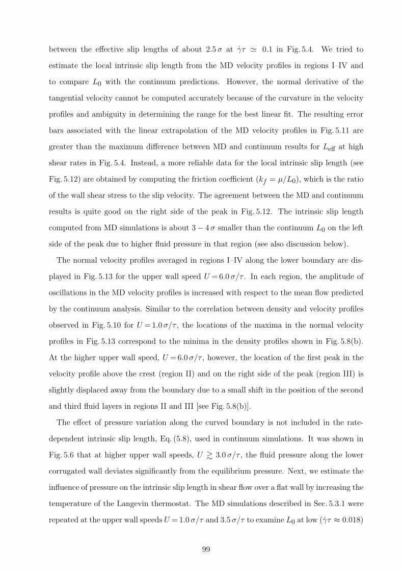
between the effective slip lengths of about 2.5 σ at γτ ' 0.1 in Fig. 5.4. We tried to

estimate the local intrinsic slip length from the MD velocity profiles in regions I–IV and

to compare L0 with the continuum predictions. However, the normal derivative of the

tangential velocity cannot be computed accurately because of the curvature in the velocity

profiles and ambiguity in determining the range for the best linear fit. The resulting error

bars associated with the linear extrapolation of the MD velocity profiles in Fig. 5.11 are

greater than the maximum difference between MD and continuum results for Leff at high

shear rates in Fig. 5.4. Instead, a more reliable data for the local intrinsic slip length (see

Fig. 5.12) are obtained by computing the friction coefficient (kf = µ/L0), which is the ratio

of the wall shear stress to the slip velocity. The agreement between the MD and continuum

results is quite good on the right side of the peak in Fig. 5.12. The intrinsic slip length

computed from MD simulations is about 3− 4 σ smaller than the continuum L0 on the left

side of the peak due to higher fluid pressure in that region (see also discussion below).

The normal velocity profiles averaged in regions I–IV along the lower boundary are dis-

played in Fig. 5.13 for the upper wall speed U = 6.0 σ/τ . In each region, the amplitude of

oscillations in the MD velocity profiles is increased with respect to the mean flow predicted

by the continuum analysis. Similar to the correlation between density and velocity profiles

observed in Fig. 5.10 for U = 1.0 σ/τ , the locations of the maxima in the normal velocity

profiles in Fig. 5.13 correspond to the minima in the density profiles shown in Fig. 5.8(b).

At the higher upper wall speed, U = 6.0 σ/τ , however, the location of the first peak in the

velocity profile above the crest (region II) and on the right side of the peak (region III) is

slightly displaced away from the boundary due to a small shift in the position of the second

and third fluid layers in regions II and III [see Fig. 5.8(b)].

The effect of pressure variation along the curved boundary is not included in the rate-

dependent intrinsic slip length, Eq. (5.8), used in continuum simulations. It was shown in

Fig. 5.6 that at higher upper wall speeds, U & 3.0 σ/τ , the fluid pressure along the lower

corrugated wall deviates significantly from the equilibrium pressure. Next, we estimate the

influence of pressure on the intrinsic slip length in shear flow over a flat wall by increasing the

temperature of the Langevin thermostat. The MD simulations described in Sec. 5.3.1 were

repeated at the upper wall speeds U = 1.0 σ/τ and 3.5 σ/τ to examine L0 at low (γτ ≈ 0.018)

99

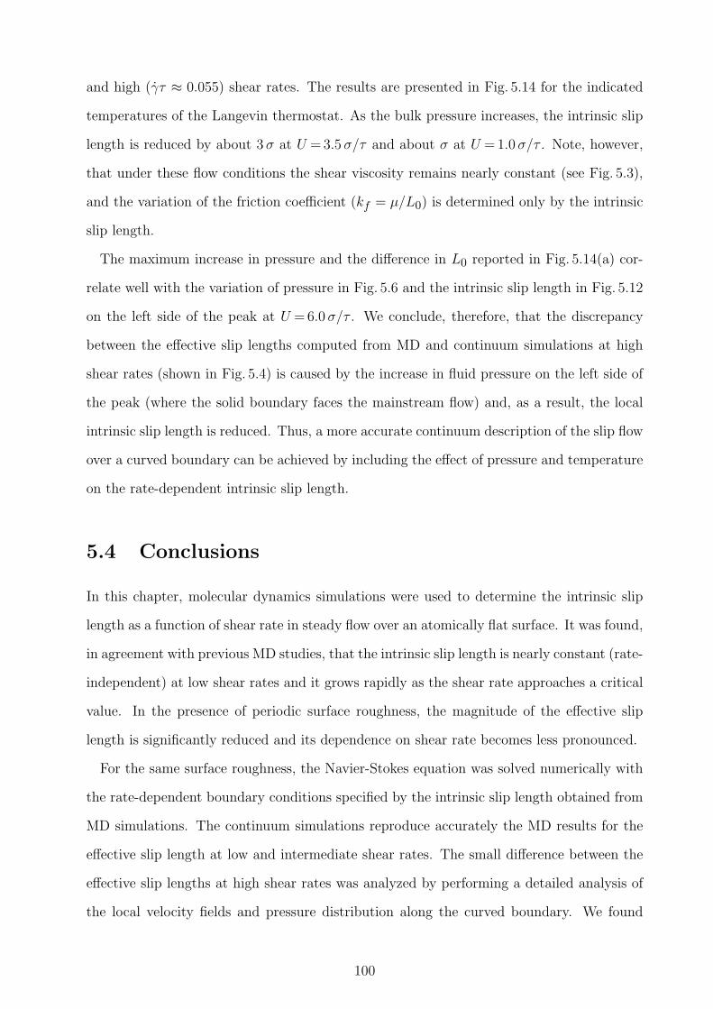
and high (γτ ≈ 0.055) shear rates. The results are presented in Fig. 5.14 for the indicated

temperatures of the Langevin thermostat. As the bulk pressure increases, the intrinsic slip

length is reduced by about 3 σ at U = 3.5 σ/τ and about σ at U = 1.0 σ/τ . Note, however,

that under these flow conditions the shear viscosity remains nearly constant (see Fig. 5.3),

and the variation of the friction coefficient (kf = µ/L0) is determined only by the intrinsic

slip length.

The maximum increase in pressure and the difference in L0 reported in Fig. 5.14(a) cor-

relate well with the variation of pressure in Fig. 5.6 and the intrinsic slip length in Fig. 5.12

on the left side of the peak at U = 6.0 σ/τ . We conclude, therefore, that the discrepancy

between the effective slip lengths computed from MD and continuum simulations at high

shear rates (shown in Fig. 5.4) is caused by the increase in fluid pressure on the left side of

the peak (where the solid boundary faces the mainstream flow) and, as a result, the local

intrinsic slip length is reduced. Thus, a more accurate continuum description of the slip flow

over a curved boundary can be achieved by including the effect of pressure and temperature

on the rate-dependent intrinsic slip length.

5.4 Conclusions

In this chapter, molecular dynamics simulations were used to determine the intrinsic slip

length as a function of shear rate in steady flow over an atomically flat surface. It was found,

in agreement with previous MD studies, that the intrinsic slip length is nearly constant (rate-

independent) at low shear rates and it grows rapidly as the shear rate approaches a critical

value. In the presence of periodic surface roughness, the magnitude of the effective slip

length is significantly reduced and its dependence on shear rate becomes less pronounced.

For the same surface roughness, the Navier-Stokes equation was solved numerically with

the rate-dependent boundary conditions specified by the intrinsic slip length obtained from

MD simulations. The continuum simulations reproduce accurately the MD results for the

effective slip length at low and intermediate shear rates. The small difference between the

effective slip lengths at high shear rates was analyzed by performing a detailed analysis of

the local velocity fields and pressure distribution along the curved boundary. We found

100

that the main cause of the discrepancy between MD and continuum results at high shear

rates is the reduction of the local intrinsic slip length in the region of higher pressure where

the boundary slope becomes relatively large with respect to the mainstream flow. These

findings suggest that the continuum analysis of the flow over a rough surface at high shear

rates should take into account the effect of pressure on the rate-dependent intrinsic slip

length. One way to include pressure in the numerical analysis is to perform an additional

set of MD simulations (for flat walls) at different values of the constant normal load and

vary the upper wall speed. Thus, the intrinsic slip length as a function pressure and shear

rate can be obtained from interpolation of the MD data and then used as a local boundary

condition in the continuum simulation.

101

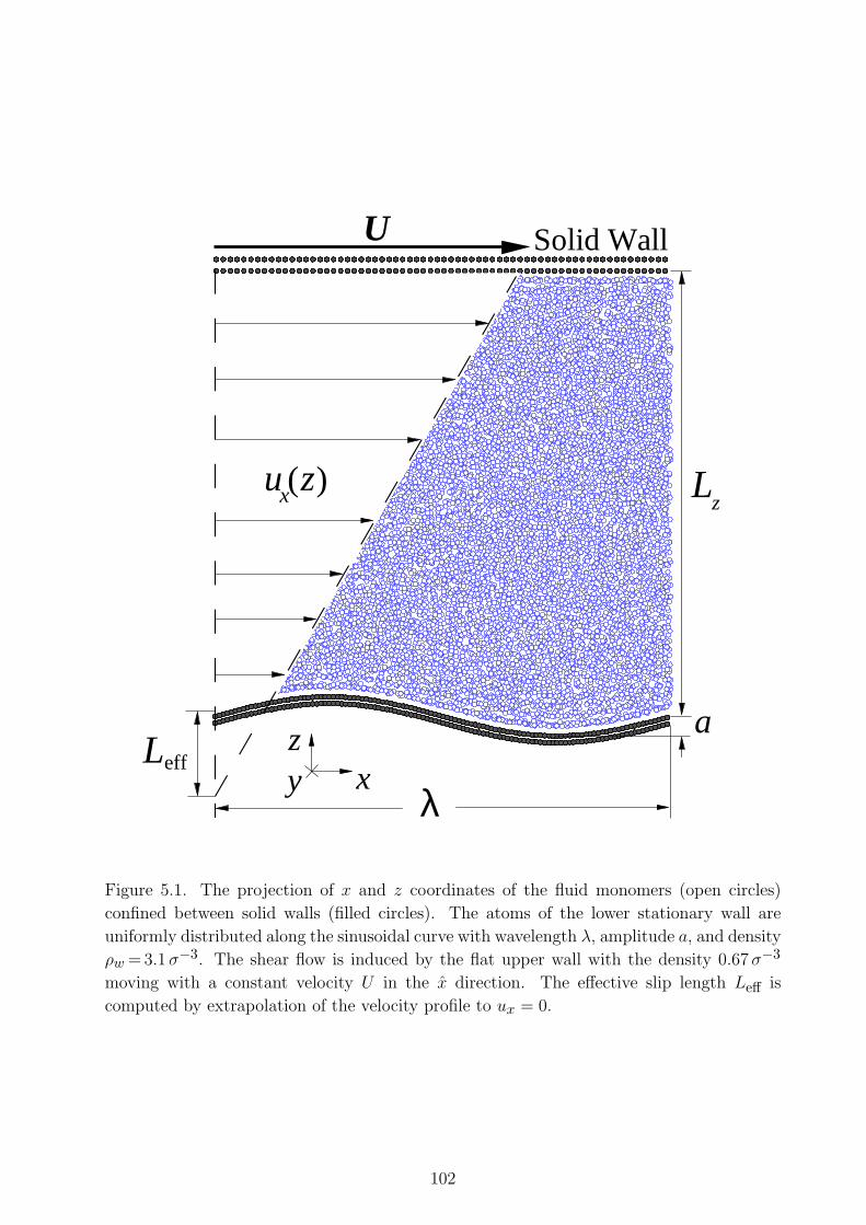
Solid WallU

λLeff

a

xzy

u z( )x Lz

Figure 5.1. The projection of x and z coordinates of the fluid monomers (open circles)

confined between solid walls (filled circles). The atoms of the lower stationary wall are

uniformly distributed along the sinusoidal curve with wavelength λ, amplitude a, and density

ρw = 3.1 σ−3. The shear flow is induced by the flat upper wall with the density 0.67 σ−3

moving with a constant velocity U in the x direction. The effective slip length Leff is

computed by extrapolation of the velocity profile to ux = 0.

102

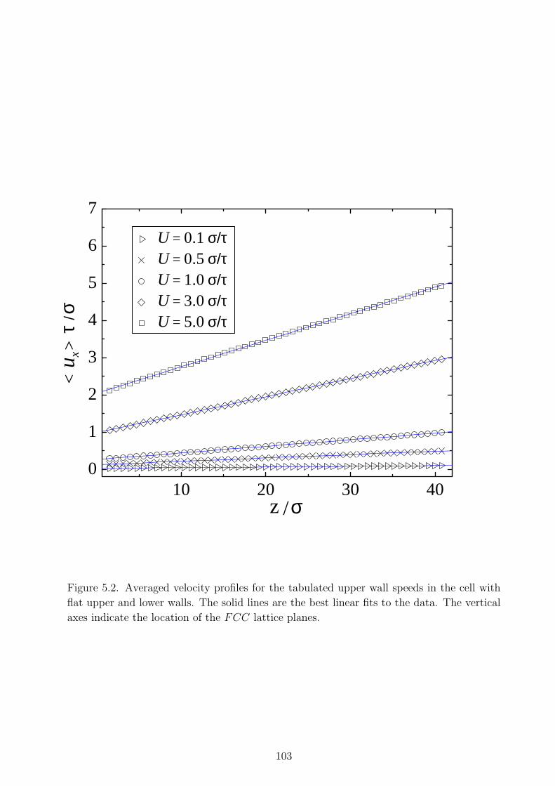
10 20 30 400

1

2

3

4

5

6

7

U = 0.1 σ/τ U = 0.5 σ/τ U = 1.0 σ/τ U = 3.0 σ/τ U = 5.0 σ/τ

σz /

< u

x> τ

/ σ

Figure 5.2. Averaged velocity profiles for the tabulated upper wall speeds in the cell with

flat upper and lower walls. The solid lines are the best linear fits to the data. The vertical

axes indicate the location of the FCC lattice planes.

103

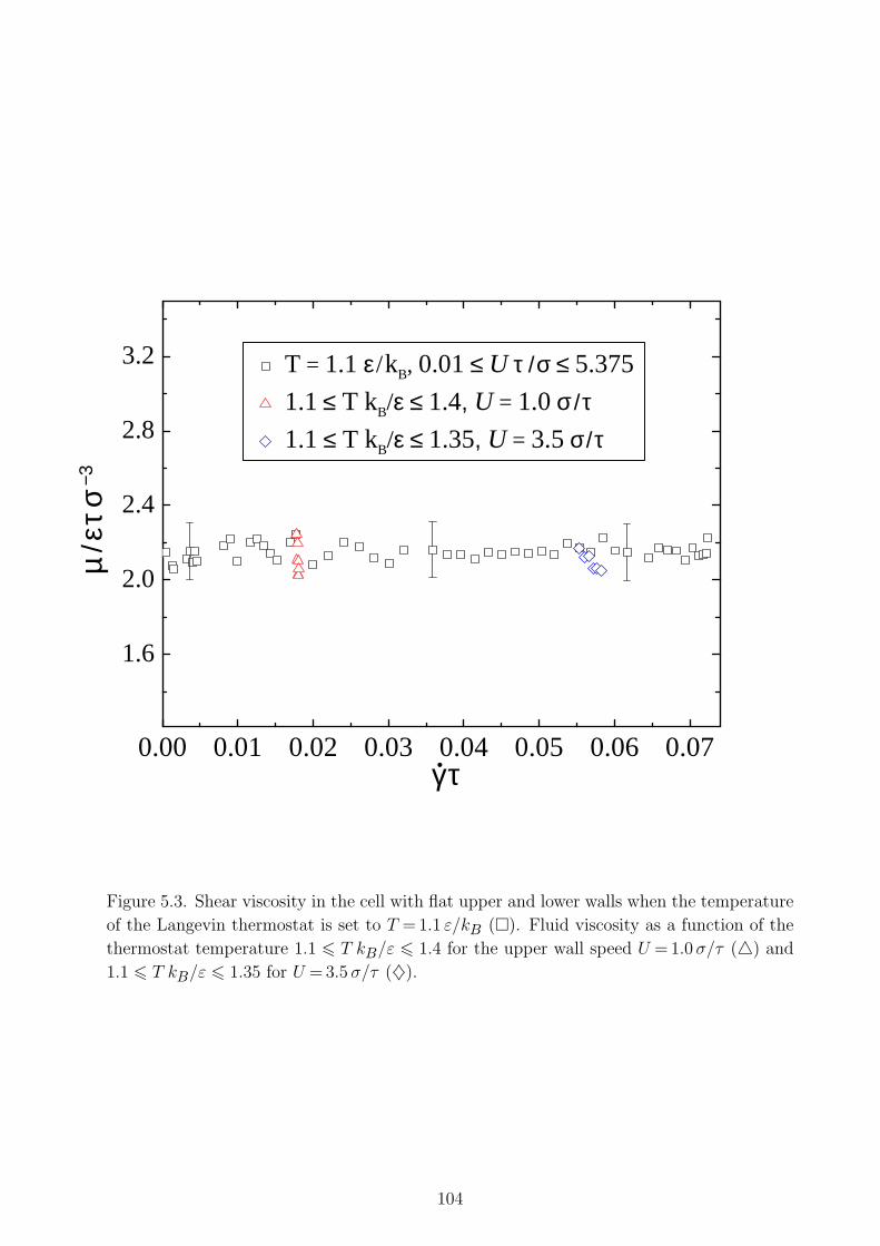
0.00 0.01 0.02 0.03 0.04 0.05 0.06 0.07

1.6

2.0

2.4

2.8

3.2 T = 1.1 ε / kB, 0.01 ≤ U τ / σ ≤ 5.375

1.1 ≤ T kB/ε ≤ 1.4, U = 1.0 σ / τ1.1 ≤ T kB/ε ≤ 1.35, U = 3.5 σ / τ

µ / ε

τ σ −

3

γ τ.

Figure 5.3. Shear viscosity in the cell with flat upper and lower walls when the temperature

of the Langevin thermostat is set to T = 1.1 ε/kB (¤). Fluid viscosity as a function of the

thermostat temperature 1.1 6 T kB/ε 6 1.4 for the upper wall speed U = 1.0 σ/τ (4) and

1.1 6 T kB/ε 6 1.35 for U = 3.5 σ/τ (♦).

104

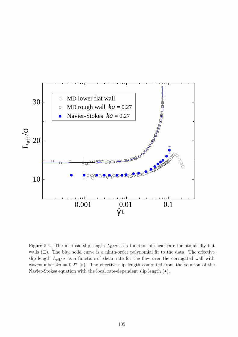
10

20

30

Lef

f /σ

MD lower flat wall MD rough wall ka = 0.27

Navier-Stokes ka = 0.27

0.10.01

γ τ. 0.001

Figure 5.4. The intrinsic slip length L0/σ as a function of shear rate for atomically flat

walls (¤). The blue solid curve is a ninth-order polynomial fit to the data. The effective

slip length Leff/σ as a function of shear rate for the flow over the corrugated wall with

wavenumber ka = 0.27 (). The effective slip length computed from the solution of the

Navier-Stokes equation with the local rate-dependent slip length (•).

105

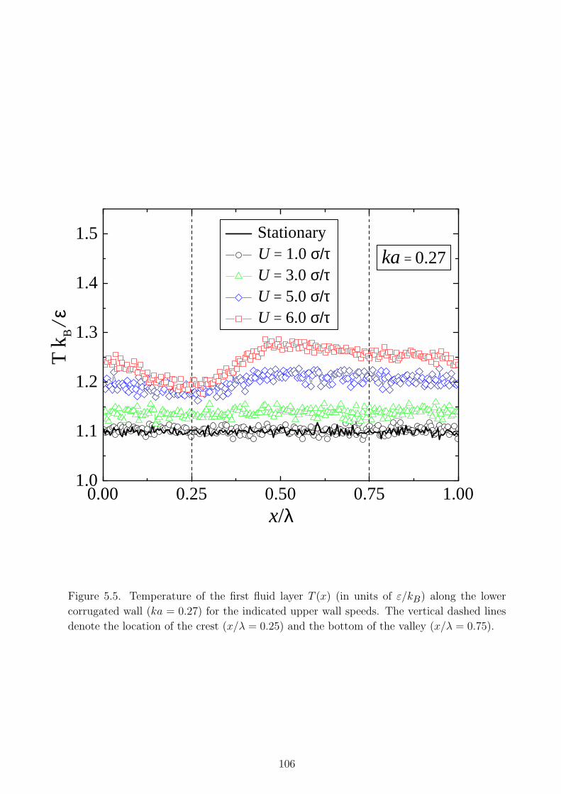
0.00 0.25 0.50 0.75 1.001.0

1.1

1.2

1.3

1.4

1.5

x/λ

T k

B / ε

Stationary U = 1.0 σ/τ U = 3.0 σ/τ U = 5.0 σ/τ U = 6.0 σ/τ

ka = 0.27

Figure 5.5. Temperature of the first fluid layer T (x) (in units of ε/kB) along the lower

corrugated wall (ka = 0.27) for the indicated upper wall speeds. The vertical dashed lines

denote the location of the crest (x/λ = 0.25) and the bottom of the valley (x/λ = 0.75).

106

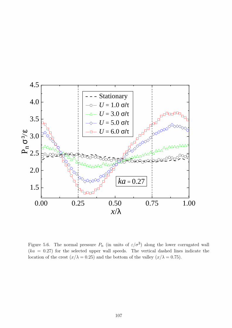
0.00 0.25 0.50 0.75 1.00

1.5

2.0

2.5

3.0

3.5

4.0

4.5

Stationary U = 1.0 σ/τ U = 3.0 σ/τ U = 5.0 σ/τ U = 6.0 σ/τ

Pn

σ 3/ ε

x/λ

ka = 0.27

Figure 5.6. The normal pressure Pn (in units of ε/σ3) along the lower corrugated wall

(ka = 0.27) for the selected upper wall speeds. The vertical dashed lines indicate the

location of the crest (x/λ = 0.25) and the bottom of the valley (x/λ = 0.75).

107

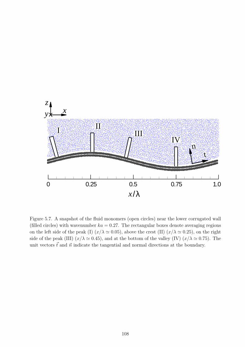
I IIIII

IV

y

x

z

nt

x

λ1.00 0.25 0.5 0.75

/

Figure 5.7. A snapshot of the fluid monomers (open circles) near the lower corrugated wall

(filled circles) with wavenumber ka = 0.27. The rectangular boxes denote averaging regions

on the left side of the peak (I) (x/λ ' 0.05), above the crest (II) (x/λ ' 0.25), on the right

side of the peak (III) (x/λ ' 0.45), and at the bottom of the valley (IV) (x/λ ' 0.75). The

unit vectors ~t and ~n indicate the tangential and normal directions at the boundary.

108

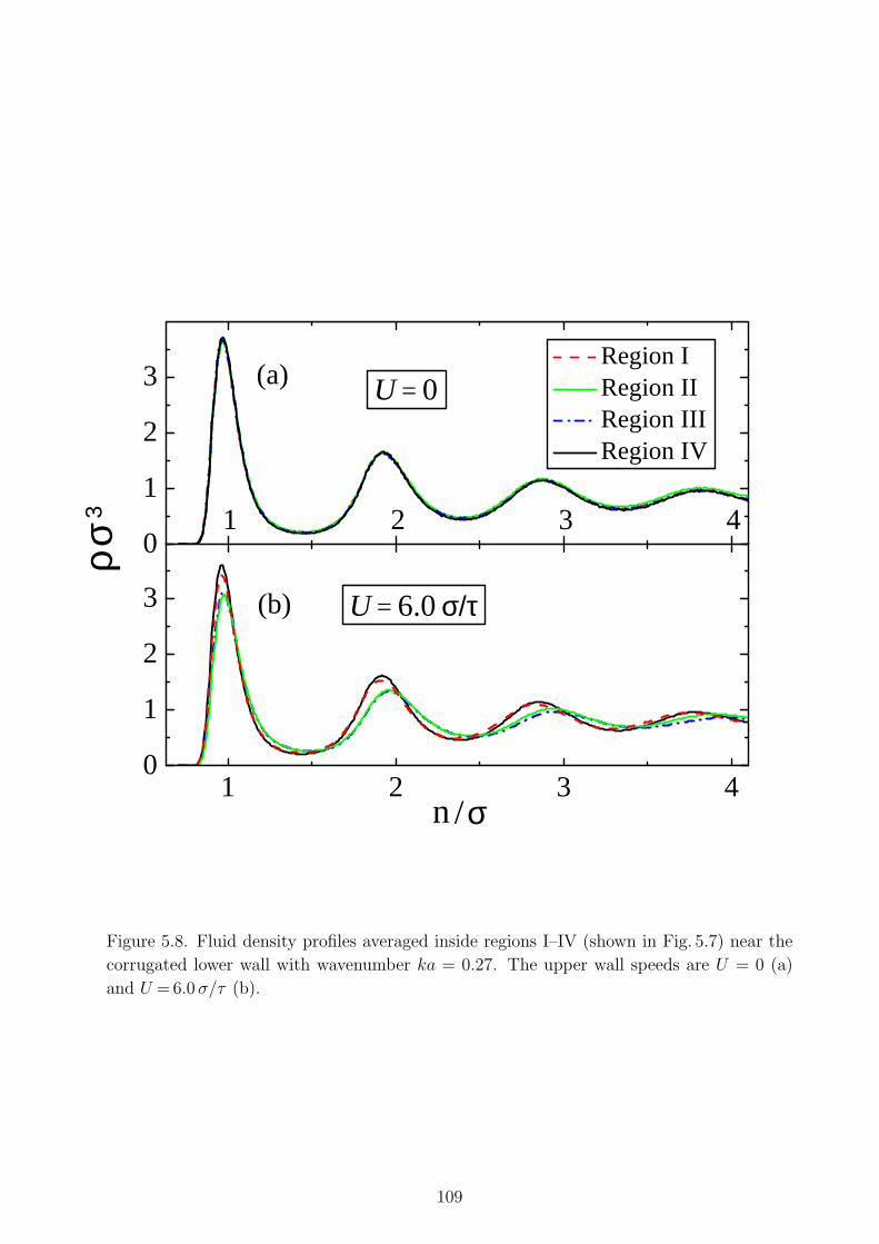
1 2 3 40

1

2

3 (b)

ρ σ 3

σn /

U = 6.0 σ/τ

1 2 3 40

1

2

3

Region I Region II Region III Region IV

(a) U = 0

Figure 5.8. Fluid density profiles averaged inside regions I–IV (shown in Fig. 5.7) near the

corrugated lower wall with wavenumber ka = 0.27. The upper wall speeds are U = 0 (a)

and U = 6.0 σ/τ (b).

109

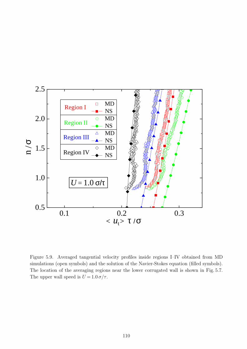
0.1 0.2 0.30.5

1.0

1.5

2.0

2.5

< ut> τ / σ

σ

n /

U = 1.0 σ/τ

MD NS MD NS MD NS MD NSRegion IV

Region II

Region I

Region III

Figure 5.9. Averaged tangential velocity profiles inside regions I–IV obtained from MD

simulations (open symbols) and the solution of the Navier-Stokes equation (filled symbols).

The location of the averaging regions near the lower corrugated wall is shown in Fig. 5.7.

The upper wall speed is U = 1.0 σ/τ .

110

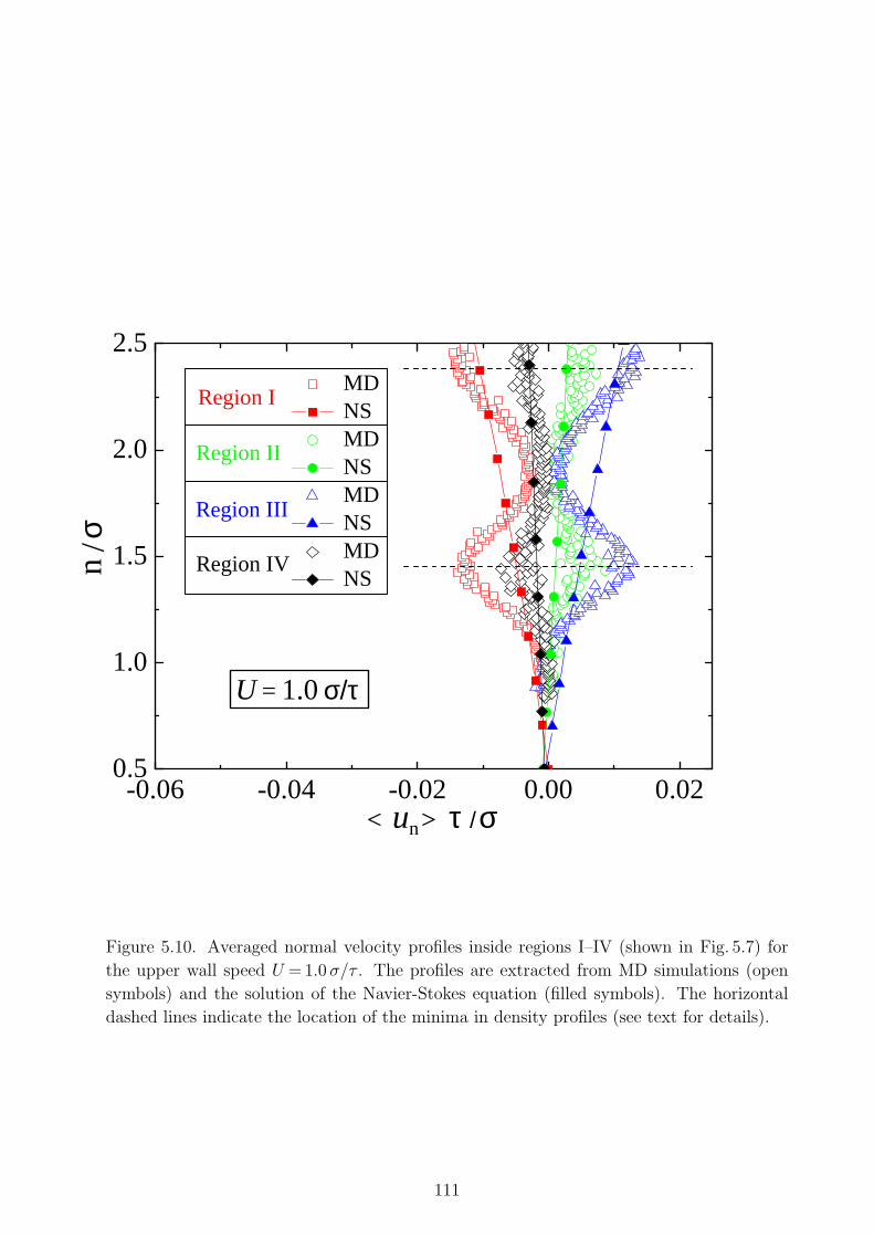
-0.06 -0.04 -0.02 0.00 0.020.5

1.0

1.5

2.0

2.5

< un> τ / σ

σn

/

U = 1.0 σ/τ

Region IV

Region II

Region I

Region III

MD NS MD NS MD NS MD NS

Figure 5.10. Averaged normal velocity profiles inside regions I–IV (shown in Fig. 5.7) for

the upper wall speed U = 1.0 σ/τ . The profiles are extracted from MD simulations (open

symbols) and the solution of the Navier-Stokes equation (filled symbols). The horizontal

dashed lines indicate the location of the minima in density profiles (see text for details).

111

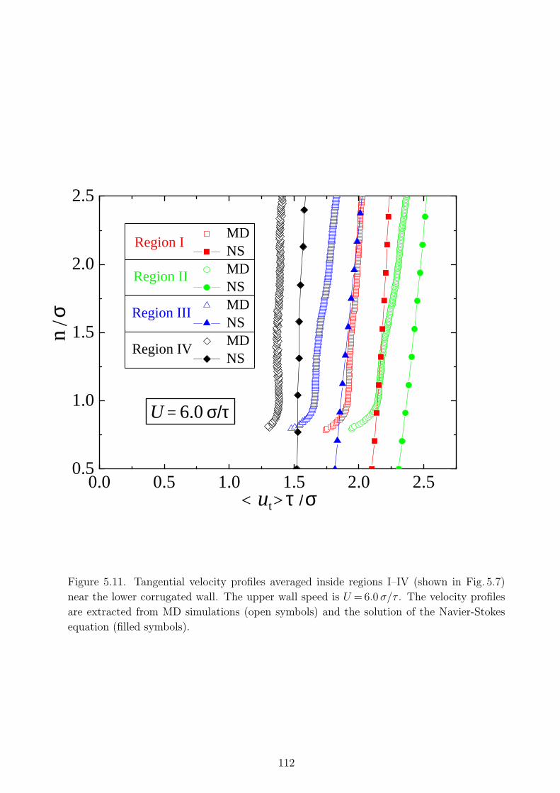
0.0 0.5 1.0 1.5 2.0 2.50.5

1.0

1.5

2.0

2.5

< ut> τ / σ

σn

/

U = 6.0 σ/τ

Region IV

Region II

Region I

Region III

MD NS MD NS MD NS MD NS

Figure 5.11. Tangential velocity profiles averaged inside regions I–IV (shown in Fig. 5.7)

near the lower corrugated wall. The upper wall speed is U = 6.0 σ/τ . The velocity profiles

are extracted from MD simulations (open symbols) and the solution of the Navier-Stokes

equation (filled symbols).

112

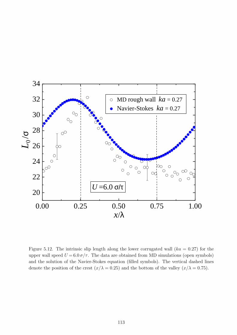
0.00 0.25 0.50 0.75 1.00

20

22

24

26

28

30

32

34

MD rough wall ka = 0.27

Navier-Stokes ka = 0.27

L0 /σ

x/λ

U =6.0 σ/τ

Figure 5.12. The intrinsic slip length along the lower corrugated wall (ka = 0.27) for the

upper wall speed U = 6.0 σ/τ . The data are obtained from MD simulations (open symbols)

and the solution of the Navier-Stokes equation (filled symbols). The vertical dashed lines

denote the position of the crest (x/λ = 0.25) and the bottom of the valley (x/λ = 0.75).

113

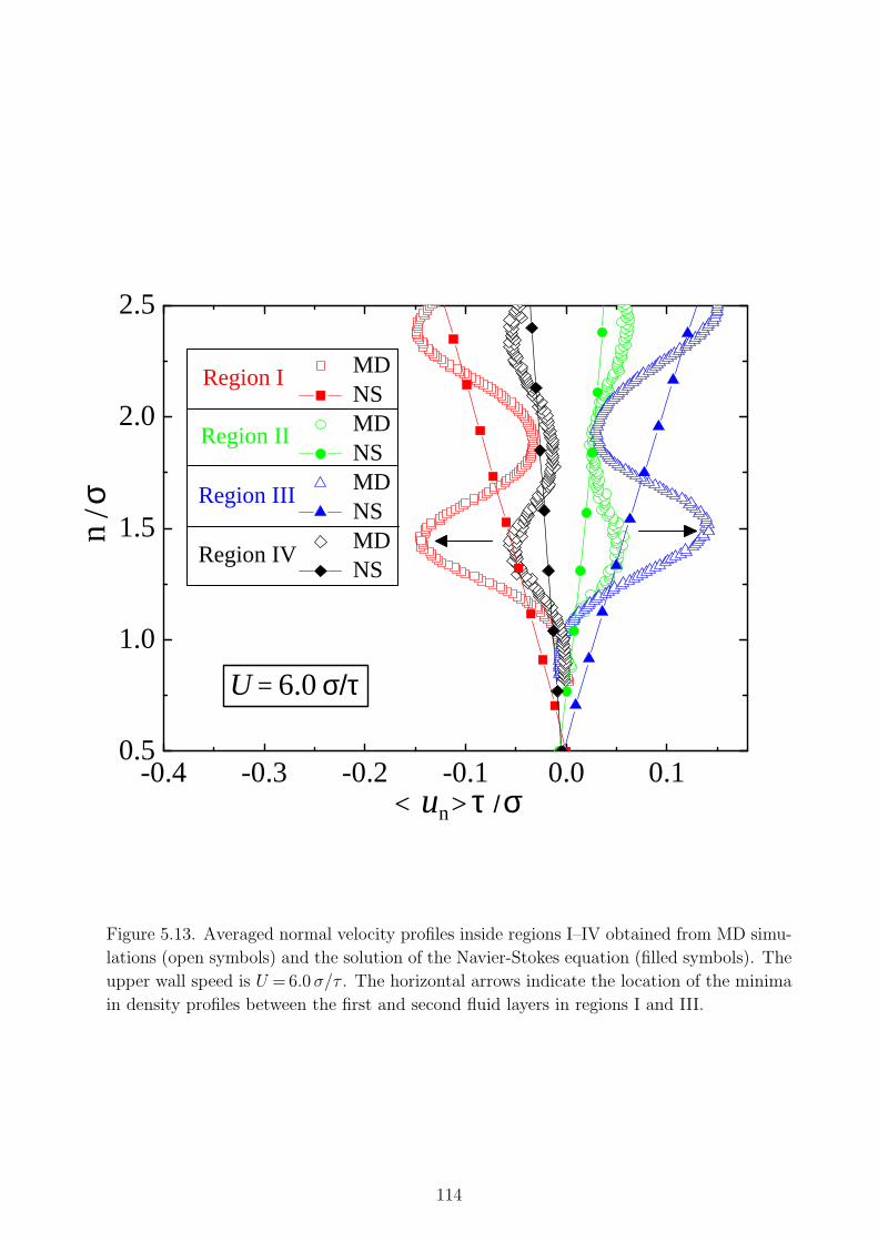
-0.4 -0.3 -0.2 -0.1 0.0 0.10.5

1.0

1.5

2.0

2.5

< un> τ / σ

σn

/

U = 6.0 σ/τ

Region IV

Region II

Region I

Region III

MD NS MD NS MD NS MD NS

Figure 5.13. Averaged normal velocity profiles inside regions I–IV obtained from MD simu-

lations (open symbols) and the solution of the Navier-Stokes equation (filled symbols). The

upper wall speed is U = 6.0 σ/τ . The horizontal arrows indicate the location of the minima

in density profiles between the first and second fluid layers in regions I and III.

114

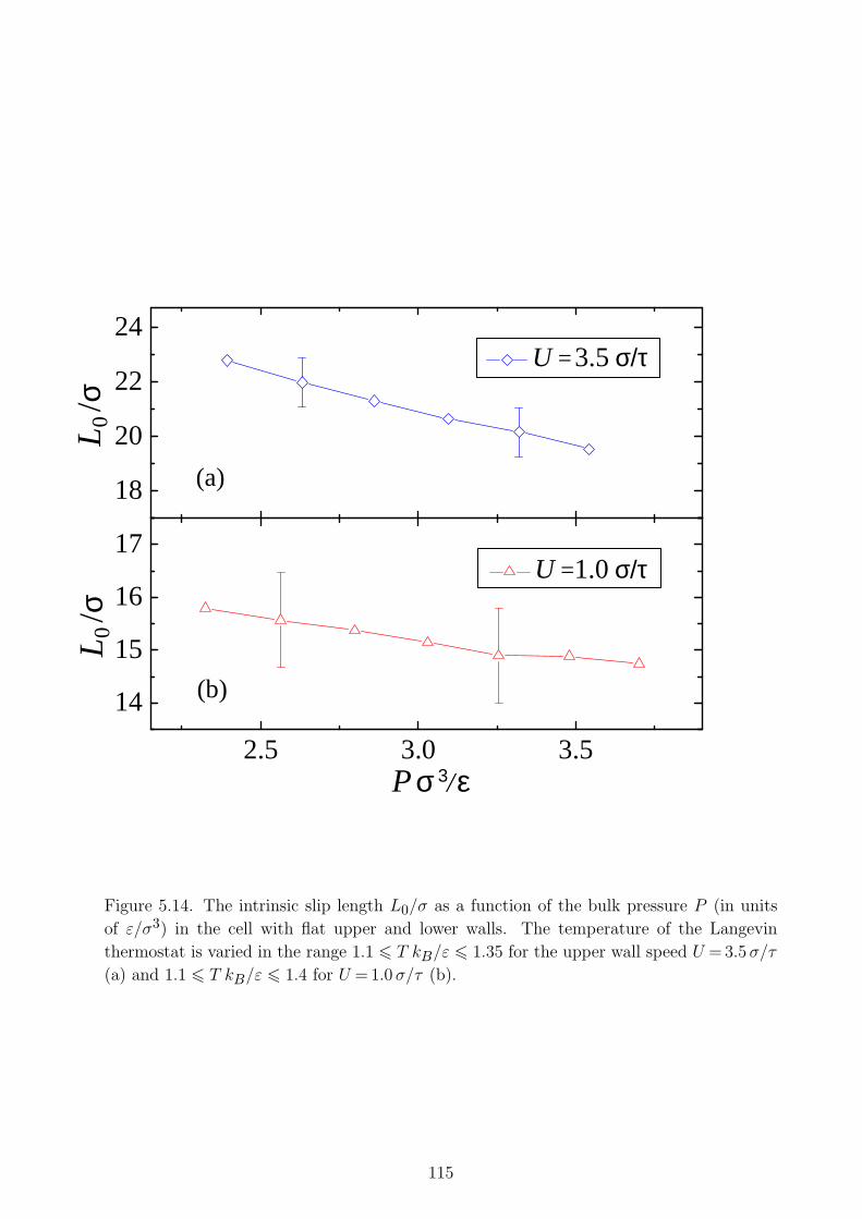
2.5 3.0 3.5

14

15

16

17 U =1.0 σ/τ

L0 /σ

P σ 3/ ε

18

20

22

24

(b)

U = 3.5 σ/τ

L0 / σ

(a)

Figure 5.14. The intrinsic slip length L0/σ as a function of the bulk pressure P (in units

of ε/σ3) in the cell with flat upper and lower walls. The temperature of the Langevin

thermostat is varied in the range 1.1 6 T kB/ε 6 1.35 for the upper wall speed U = 3.5 σ/τ

(a) and 1.1 6 T kB/ε 6 1.4 for U = 1.0 σ/τ (b).

115

CHAPTER 6

Slip boundary conditions for the

moving contact line in molecular

dynamics and continuum simulations

6.1 Introduction

The problem of contact line motion, which involves flow of two immiscible viscous fluids

in contact with a solid substrate, has captivated a lot of attention because of its funda-

mental difficulties and important applications including droplet spreading, spray painting,

lubrication, and coating [134, 135].

In wetting problems, the line of contact of the fluid/fluid interface with the solid wall

is called the contact line. In the absence of the fluid flow relative to the solid wall, the

fluid/fluid interface forms an angle with the solid wall, called the static contact angle θs,

which is determined by the balance of the surface tensions between three media. In the

presence of flow, the shape of the fluid/fluid interface near the wall becomes deformed and

it is described by the dynamic contact angle θd. The deformation of the interface depends on

the flow fields near the contact line, surface tensions, and energy dissipation at the contact

line.

The analytical calculation of flow fields and motion of the contact line with no-slip bound-

ary condition along the solid surface leads to a stress singularity and infinite viscous dissipa-

116

tion near the contact line [136, 137]. Due to multi-scale nature of the moving contact line

problem and breakdown of the local hydrodynamics near the contact point, the problem has

inspired many theoretical/numerical studies over the last 30 years [62, 137, 138, 141, 144].

On the other hand, experimental studies are limited to measuring a macroscopic contact

angle, known also as an apparent contact angle θa, which is accessible at a distance R (order

of microns) from the surface. When the shape of the fluid/fluid interface is deformed on a

molecular distance from the wall, the static contact angle θs and dynamic contact angle θd

are distinguishable while θa depends on the value of R.

Most of analytical and numerical solutions of the moving contact line problem were per-

formed based on the fact that the far field solution of the problem is almost insensitive

to the exact dynamics of the contact line close to wall [138]. One of the possibilities to

remove the singularity at the contact line is to replace the no-slip boundary condition with

slip BC via the Navier model. Some of the challenges in applying the slip models near the

fluid/solid interface include a correct specification of the region near the contact line where

the boundary slip must be applied, the magnitude of the slip length, and the shape of the

fluid/fluid interface.

The molecular dynamics (MD) simulations have been only recently used to study the

moving contact line problem [20, 130, 131, 139, 140, 141, 142, 143, 144, 145]. One of the

advantages of the MD method is that it offers a detailed information about microscopic

flow structure near the contact line without any assumptions about boundary conditions or

constitutive relations. Thus, an accurate physical description of the flow fields and motion of

the contact line can be obtained from MD simulations, which in turn might help to develop

models for characterizing the flow behavior in continuum modeling.

In this chapter, the moving contact line problem is studied using a combined approach of

molecular dynamics and continuum simulations. First, MD simulations are carried out to

resolve the flow fields in the vicinity of the moving contact line on the molecular scale and

to establish a relation between the interfacial shear stresses and slip length as a function of

the distance from the contact line. This is done by extracting the velocity profiles and the

shear and normal stress tensors at the fluid/solid interface. Second, in the presence of shear

flow, the shape of the fluid/fluid interface is accurately resolved using MD simulations. In

117

the next step, the boundary conditions near the moving contact line extracted from MD

simulations are implemented as input conditions in the continuum solution of the Navier-

Stokes equation (using the finite difference/particle tracking methods) to reproduce velocity

profiles and the shape of the fluid/fluid interface.

The rest of this chapter is organized as follows. The details of MD simulations, equili-

bration procedure, careful evaluation of normal stresses near the solid substrate, averaging

velocity profiles are presented in the Sec. 6.2. The continuum model and comparative analy-

sis are described in Sec. 6.3. A brief summary is given in the last section.

6.2 Molecular dynamics (MD) simulations

6.2.1 Equilibrium case

The system consists of two immiscible fluids confined between flat walls. The initial config-

uration of the atoms is presented in Fig. 6.3. Each of two solid walls is modeled as two layers

of FCC lattice in [111] direction. The number of fluid monomers in fluid 1 and 2 are fixed

to Nf1 = 18900 and Nf2 = 18900, respectively. The total number of wall atoms is set to

Nw = 10600. The MD simulations were performed at a constant fluid density (ρ = 0.81 σ−3)

ensemble, while the wall density is set to ρw = 1.86 σ−3 to allow a partial slip flow along the

walls in each single fluid phase. The thermostat temperature is set to T = 1.1 ε/kB , where

kB is the Boltzmann constant. The system size in the x and y directions is Lx = 241.87 σ

and Ly = 7.90 σ. The relative distance between the walls is fixed to Lz = 25.41 σ in the z

direction. Periodic boundary conditions were applied along the x and y directions.

The fluid monomers interact through the truncated pairwise Lennard-Jones (LJ) potential

VLJ (r) = 4ε[(σ

r

)12 − δ(σ

r

)6], (6.1)

where ε is the energy scale and σ is the length scale of the fluid phase. The cutoff radius for

the LJ potential is set to rc = 2.5 σ for the fluid/fluid and wall/fluid interactions. For the

contact line problem, the LJ potential is modified by adding a parameter δ in the attractive

part of the potential. For fluid 1/fluid 1, fluid 2/fluid 2, and wall/fluid interactions δ = 1.

However, for immiscible fluids (fluid 1/fluid 2), δ = −1 and the LJ potential only consists

118

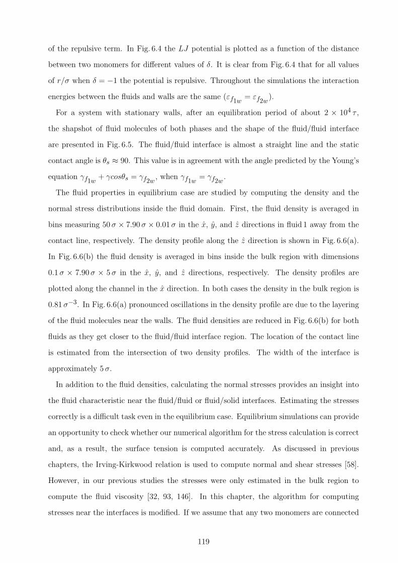
of the repulsive term. In Fig. 6.4 the LJ potential is plotted as a function of the distance

between two monomers for different values of δ. It is clear from Fig. 6.4 that for all values

of r/σ when δ = −1 the potential is repulsive. Throughout the simulations the interaction

energies between the fluids and walls are the same (εf1w= εf2w

).

For a system with stationary walls, after an equilibration period of about 2 × 104 τ ,

the shapshot of fluid molecules of both phases and the shape of the fluid/fluid interface

are presented in Fig. 6.5. The fluid/fluid interface is almost a straight line and the static

contact angle is θs ≈ 90. This value is in agreement with the angle predicted by the Young’s

equation γf1w+ γcosθs = γf2w , when γf1w

= γf2w.

The fluid properties in equilibrium case are studied by computing the density and the

normal stress distributions inside the fluid domain. First, the fluid density is averaged in

bins measuring 50 σ × 7.90 σ × 0.01 σ in the x, y, and z directions in fluid 1 away from the

contact line, respectively. The density profile along the z direction is shown in Fig. 6.6(a).

In Fig. 6.6(b) the fluid density is averaged in bins inside the bulk region with dimensions

0.1 σ × 7.90 σ × 5 σ in the x, y, and z directions, respectively. The density profiles are

plotted along the channel in the x direction. In both cases the density in the bulk region is

0.81 σ−3. In Fig. 6.6(a) pronounced oscillations in the density profile are due to the layering

of the fluid molecules near the walls. The fluid densities are reduced in Fig. 6.6(b) for both

fluids as they get closer to the fluid/fluid interface region. The location of the contact line

is estimated from the intersection of two density profiles. The width of the interface is

approximately 5 σ.

In addition to the fluid densities, calculating the normal stresses provides an insight into

the fluid characteristic near the fluid/fluid or fluid/solid interfaces. Estimating the stresses

correctly is a difficult task even in the equilibrium case. Equilibrium simulations can provide

an opportunity to check whether our numerical algorithm for the stress calculation is correct

and, as a result, the surface tension is computed accurately. As discussed in previous

chapters, the Irving-Kirkwood relation is used to compute normal and shear stresses [58].

However, in our previous studies the stresses were only estimated in the bulk region to

compute the fluid viscosity [32, 93, 146]. In this chapter, the algorithm for computing

stresses near the interfaces is modified. If we assume that any two monomers are connected

119

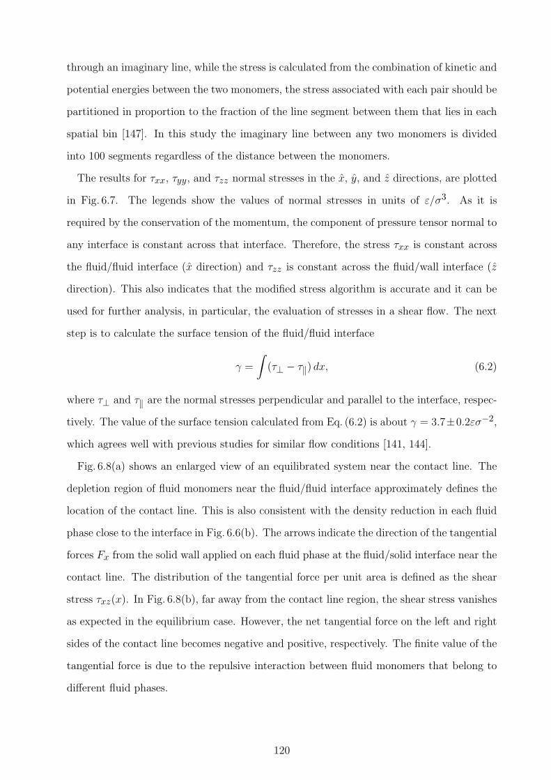
through an imaginary line, while the stress is calculated from the combination of kinetic and

potential energies between the two monomers, the stress associated with each pair should be

partitioned in proportion to the fraction of the line segment between them that lies in each

spatial bin [147]. In this study the imaginary line between any two monomers is divided

into 100 segments regardless of the distance between the monomers.

The results for τxx, τyy, and τzz normal stresses in the x, y, and z directions, are plotted

in Fig. 6.7. The legends show the values of normal stresses in units of ε/σ3. As it is

required by the conservation of the momentum, the component of pressure tensor normal to

any interface is constant across that interface. Therefore, the stress τxx is constant across

the fluid/fluid interface (x direction) and τzz is constant across the fluid/wall interface (z

direction). This also indicates that the modified stress algorithm is accurate and it can be

used for further analysis, in particular, the evaluation of stresses in a shear flow. The next

step is to calculate the surface tension of the fluid/fluid interface

γ =

∫(τ⊥ − τ‖) dx, (6.2)

where τ⊥ and τ‖ are the normal stresses perpendicular and parallel to the interface, respec-

tively. The value of the surface tension calculated from Eq. (6.2) is about γ = 3.7±0.2εσ−2,

which agrees well with previous studies for similar flow conditions [141, 144].

Fig. 6.8(a) shows an enlarged view of an equilibrated system near the contact line. The

depletion region of fluid monomers near the fluid/fluid interface approximately defines the

location of the contact line. This is also consistent with the density reduction in each fluid

phase close to the interface in Fig. 6.6(b). The arrows indicate the direction of the tangential

forces Fx from the solid wall applied on each fluid phase at the fluid/solid interface near the

contact line. The distribution of the tangential force per unit area is defined as the shear

stress τxz(x). In Fig. 6.8(b), far away from the contact line region, the shear stress vanishes

as expected in the equilibrium case. However, the net tangential force on the left and right

sides of the contact line becomes negative and positive, respectively. The finite value of the

tangential force is due to the repulsive interaction between fluid monomers that belong to

different fluid phases.

120

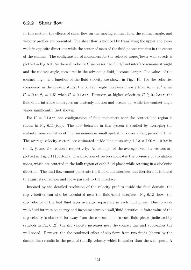
6.2.2 Shear flow

In this section, the effects of shear flow on the moving contact line, the contact angle, and

velocity profiles are presented. The shear flow is induced by translating the upper and lower

walls in opposite directions while the center of mass of the fluid phases remains in the center

of the channel. The configuration of monomers for the selected upper/lower wall speeds is

plotted in Fig. 6.9. As the wall velocity U increases, the fluid/fluid interface remains straight

and the contact angle, measured in the advancing fluid, becomes larger. The values of the

contact angle as a function of the fluid velocity are shown in Fig. 6.10. For the velocities

considered in the present study, the contact angle increases linearly from θs = 90 when

U = 0 to θd = 115 when U = 0.1 σ/τ . However, at higher velocities, U & 0.12 σ/τ , the

fluid/fluid interface undergoes an unsteady motion and breaks up, while the contact angle

varies significantly (not shown).

For U = 0.1 σ/τ , the configuration of fluid monomers near the contact line region is

shown in Fig. 6.11 (top). The flow behavior in this system is studied by averaging the

instantaneous velocities of fluid monomers in small spatial bins over a long period of time.

The average velocity vectors are estimated inside bins measuring 1.0 σ × 7.90 σ × 0.9 σ in

the x, y, and z directions, respectively. An example of the averaged velocity vectors are

plotted in Fig. 6.11 (bottom). The direction of vectors indicates the presence of circulation

zones, which are centered in the bulk region of each fluid phase while rotating in a clockwise

direction. The fluid flow cannot penetrate the fluid/fluid interface, and therefore, it is forced

to adjust its direction and move parallel to the interface.

Inspired by the detailed resolution of the velocity profiles inside the fluid domain, the

slip velocities can also be calculated near the fluid/solid interface. Fig. 6.12 shows the

slip velocity of the first fluid layer averaged separately in each fluid phase. Due to weak

wall/fluid interaction energy and incommensurable wall/fluid densities, a finite value of the

slip velocity is observed far away from the contact line. In each fluid phase (indicated by

symbols in Fig. 6.12), the slip velocity increases near the contact line and approaches the

wall speed. However, the the combined effect of slip flows from two fluids (shown by the

dashed line) results in the peak of the slip velocity which is smaller than the wall speed. A

121

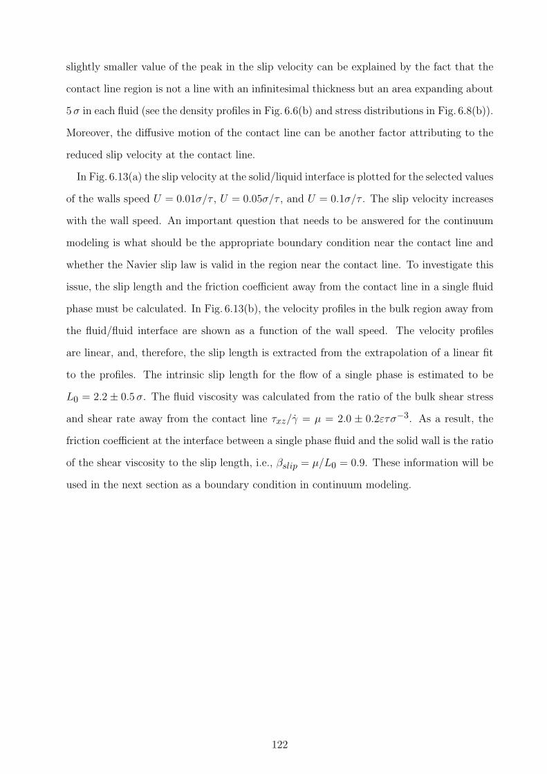
slightly smaller value of the peak in the slip velocity can be explained by the fact that the

contact line region is not a line with an infinitesimal thickness but an area expanding about

5 σ in each fluid (see the density profiles in Fig. 6.6(b) and stress distributions in Fig. 6.8(b)).

Moreover, the diffusive motion of the contact line can be another factor attributing to the

reduced slip velocity at the contact line.

In Fig. 6.13(a) the slip velocity at the solid/liquid interface is plotted for the selected values

of the walls speed U = 0.01σ/τ , U = 0.05σ/τ , and U = 0.1σ/τ . The slip velocity increases

with the wall speed. An important question that needs to be answered for the continuum

modeling is what should be the appropriate boundary condition near the contact line and

whether the Navier slip law is valid in the region near the contact line. To investigate this

issue, the slip length and the friction coefficient away from the contact line in a single fluid

phase must be calculated. In Fig. 6.13(b), the velocity profiles in the bulk region away from

the fluid/fluid interface are shown as a function of the wall speed. The velocity profiles

are linear, and, therefore, the slip length is extracted from the extrapolation of a linear fit

to the profiles. The intrinsic slip length for the flow of a single phase is estimated to be

L0 = 2.2± 0.5 σ. The fluid viscosity was calculated from the ratio of the bulk shear stress

and shear rate away from the contact line τxz/γ = µ = 2.0 ± 0.2ετσ−3. As a result, the

friction coefficient at the interface between a single phase fluid and the solid wall is the ratio

of the shear viscosity to the slip length, i.e., βslip = µ/L0 = 0.9. These information will be

used in the next section as a boundary condition in continuum modeling.

122

6.3 Details of continuum simulations

In moving boundary problems the interface treatment including shape, location, and ve-

locity is highly complicated because the information on the interface need to be computed

along with the field equations. Numerous techniques exist for tracking moving interfaces.

These techniques can be classified under three main categories a) moving grid (Lagrangian)

methods, b) Eulerian methods, and c) combined Lagrangian-Eulerian methods. All these

approaches have their relative merits and none of them is superior for all applications.

In this section, the problem of the contact line motion is modeled using a Lagrangian-

Eulerian algorithm. The Navier-Stokes (N-S) equations are solved with the finite difference

method on a fixed Eulerian grid combined with tracking Lagrangian marker points assigned

on the fluid/fluid interface. The N-S equations provide the description of the pressure and

velocity distributions in the fluid domain [149]. The marker points determine the time

evolution of the fluid/fluid interface [150]. Meanwhile, the molecular dynamics simulations

provide correct boundary conditions near the contact line (i.e., the slip length, shear stresses,

and friction coefficients).

6.3.1 Fixed grid method for immersed objects

This method operates on a fixed Cartesian mesh (Eulerian part) while the fluid/fluid inter-

faces move through the mesh (Lagrangian part). The advantage of the fixed grid approach

is that the grid topology remains simple while large distortions of the interface take place.

In the immersed boundary method, originally used by Peskin [148] to model heart flows,

the interface can be handled via a set of marker points.

Interface

Consider a fluid domain, which is covered with a fixed Cartesian grid. The interface between

Fluid 1 and Fluid 2 represented by a curve C. The grid spacing is h. The immersed boundary

denoted by C(t) (a curve in 2D case) is represented by k markers or interfacial points with

coordinate ~xk(s) with k = 1, 2, ..., K. The markers are uniformly distributed along C(t) at

a fraction of the grid spacing, 0.5 < ds < 1.5h. The fluid/fluid interface is parameterized as

123

a function of the arclength s by fitting a local cubic polynomial to every four neighboring

points. Once the interface position is known, the normal vector and curvature are evaluated

and the material properties in each fluid are assigned. The normal vector in 2D is given by

nx = − ys√x2

s + y2s

and ny =xs√

x2s + y2

s

, (6.3)

where subscript s denotes d/ds. The curvature is then obtained by taking the divergent of

the normal vector:

κ = ~∇ · ~n. (6.4)

Knowing the interface location with respect to the grid system, the material properties

are assigned in each fluid phase based on a Heaviside step function:

β = β1 + (β2 − β1)H(~x− ~xk), (6.5)

where β is the material property such as ρ density and µ shear viscosity. The subscripts

1 and 2 denote Fluid 1 and Fluid 2, respectively. The function H(~x − ~xk) is the discrete

Heaviside step function defined as:

H(~x− ~xk) =

dim∏

m=1

1

2

(1 +

(~xm − (~xm)k)

d+

1

πsin

π(~xm − (~xm)k)

d

)if |~x− ~xk| 6 d

1 if ~x− ~xk > +d

0 if ~x− ~xk < −d

,

(6.6)

where dim is the spatial dimension, d = 2h with h is the grid spacing, ~x is the grid coordinate,

and ~xk is the interfacial marker coordinate. The Heaviside step function allows a smooth

distribution of the material properties over a transition zone d. The transition zone is twice

the grid spacing d = 2h. Therefore, the interface has the finite thickness d. Once the

material properties are assigned to each fluid, the fluid flow equations can be solved.

Immersed boundary treatment

The immersed boundary technique facilitates the communication between the moving mark-

ers, which represent the interface and the fixed grid. In particular, since the location of the

marker points does not coincide with the grid points, the velocity field stored at the cell-

center of each grid is interpolated to obtain the velocity of the interface points, and the

124

interface forces acting on the marker points is distributed to the nearby grid points using a

discrete Delta function. The Delta function is given by:

δ(~x− ~xk) =

dim∏

m=1

1

2d

(1 + cos

π(~xm − (~xm)k)

d

)if |~x− ~xk| 6 d

0 otherwise

. (6.7)

The delta function is the derivative of the Heaviside function and typically spreads over

the region of 4h.

Estimation of the force ~F : The force exerted by the fluid/fluid interface on the flow is

added to the momentum equation. The integral of the source terms is expressed as:

~F =

∫

C(t)γκnδ(~x− ~xk)ds, (6.8)

where the integral is taken over C(t), γ is the surface tension, κ is the curvature, n is the

normal unit vector, δ(~x− ~xk) is the ’Dirac’ Delta function, ~x gives the location of the grid

points, ~xk gives the position of the markers as a function of arclength s. In the discretized

form, the force is estimated by:

~Fp =∑

k

γκknkδ(~x− ~xk)∆sk, (6.9)

The force at the point P , Fp, is evaluated based on the summation of all interfacial forces

of the marker points located inside a circle of radius 2h weighted by the Delta function.

Estimation of the interface velocity ~Uk: The velocity of a marker point or interface veloc-

ity denoted by ~Uk should satisfy the continuity condition. So ~Uk is:

~Uk =

∫

Ω~u δ(~x− ~xk)d~x, (6.10)

where the integral is over the entire fluid domain Ω, ~u is the fluid velocity vector, and

δ(~x− ~xk) is the Delta function. In the discretized form, the velocity of the marker point is:

~Uk =∑

ij

~uijδ(~x− ~xk)h2, (6.11)

where h is the grid spacing, i and j are the grid indices and ~u is the fluid velocity. The

velocity at the kth marker, ~Uk, is the sum of the fluid velocity of the grid points located

inside a circle of radius 2h, weighted by the Delta function.

125

The interface velocity ~Uk is by definition the time derivative of the marker point position:

~Uk =∂~x

∂t. (6.12)

Therefore, the interface is advected as:

~xn+1k = ~xn

k +4t(~Unk ). (6.13)

The dynamics of two immiscible fluids in a channel is governed by the incompressible

Navier-Stokes equations given below

∇ · u = 0, (6.14)

∂(ρu)

∂t+∇ · (uρu) = −∇p + µ∇2u + F. (6.15)

In these equations u is the fluid velocity vector, p the pressure, F the body force, µ the

dynamic viscosity of fluid, ρ the density of fluid, and t time. The properties are constant in

each fluid.

The Navier-Stokes equations are solved using the projection method on fixed Cartesian

grids. The projection method is divided into three steps:

Step1: Solve the momentum equations without pressure. Evaluation of the intermediate

velocities ux and uz for a two dimensional problem:

( u − un

∆t

)+

(3(u · ∇u)n − (u · ∇u)n−1

2

)=

ν∇2un − ν∇2u

2+ F, (6.16)

where n is the time step level and F is the source term.

The pressure equation is derived by assuming that the velocity satisfies the continuity

equation at n + 1 time step level.

Step 2: The following equation is solved for the pressure

∇ · un+1 = 0 ⇒ ∇ · (1ρ∇pn+1) =

1

∆t∇ · u . (6.17)

Step 3: Combining the velocity and pressure information: Finally, the correction step is

done as follows

un+1 = u −∆t(1

ρ∇pn+1). (6.18)

126

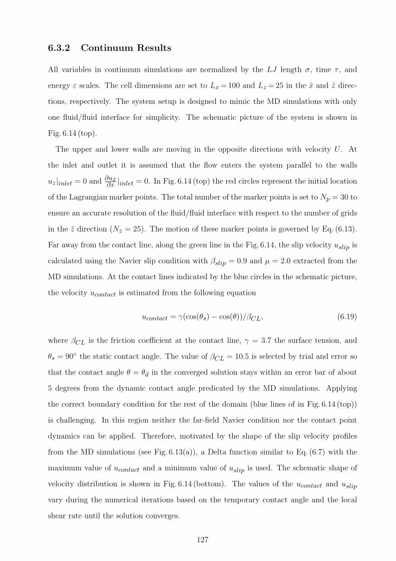
6.3.2 Continuum Results

All variables in continuum simulations are normalized by the LJ length σ, time τ , and

energy ε scales. The cell dimensions are set to Lx = 100 and Lz = 25 in the x and z direc-

tions, respectively. The system setup is designed to mimic the MD simulations with only

one fluid/fluid interface for simplicity. The schematic picture of the system is shown in

Fig. 6.14 (top).

The upper and lower walls are moving in the opposite directions with velocity U . At

the inlet and outlet it is assumed that the flow enters the system parallel to the walls

uz|inlet = 0 and ∂ux∂x |inlet = 0. In Fig. 6.14 (top) the red circles represent the initial location

of the Lagrangian marker points. The total number of the marker points is set to Np = 30 to

ensure an accurate resolution of the fluid/fluid interface with respect to the number of grids

in the z direction (Nz = 25). The motion of these marker points is governed by Eq. (6.13).

Far away from the contact line, along the green line in the Fig. 6.14, the slip velocity uslip is

calculated using the Navier slip condition with βslip = 0.9 and µ = 2.0 extracted from the

MD simulations. At the contact lines indicated by the blue circles in the schematic picture,

the velocity ucontact is estimated from the following equation

ucontact = γ(cos(θs)− cos(θ))/βCL, (6.19)

where βCL is the friction coefficient at the contact line, γ = 3.7 the surface tension, and

θs = 90 the static contact angle. The value of βCL = 10.5 is selected by trial and error so

that the contact angle θ = θd in the converged solution stays within an error bar of about

5 degrees from the dynamic contact angle predicated by the MD simulations. Applying

the correct boundary condition for the rest of the domain (blue lines of in Fig. 6.14 (top))

is challenging. In this region neither the far-field Navier condition nor the contact point

dynamics can be applied. Therefore, motivated by the shape of the slip velocity profiles

from the MD simulations (see Fig. 6.13(a)), a Delta function similar to Eq. (6.7) with the

maximum value of ucontact and a minimum value of uslip is used. The schematic shape of

velocity distribution is shown in Fig. 6.14 (bottom). The values of the ucontact and uslip

vary during the numerical iterations based on the temporary contact angle and the local

shear rate until the solution converges.

127

The velocity vectors and the streamlines are shown in Fig. 6.15 for U = 0.01, U = 0.05,

and U = 0.1. The streamline directions indicate that the fluid can not penetrate into the

contact region, and, therefore, a circulation zone is formed in each side of the contact line,

which is shown by a red line. The dynamic contact angle as a function of the wall speed is

plotted in Fig. 6.16 and the results are compared with MD simulations. The dynamic contact

angle in the advancing fluid phase increases with increasing wall speed. As discussed earlier

in Sec. 6.2 and shown in the Fig. 6.16, the value of the friction coefficient βCL was chosen

to keep the contact angle extracted from the Navier-Stokes solution within an error bar of

about 5 from the MD results.

The slip velocity profiles from the Navier-Stokes solution are plotted in Fig. 6.17 by sym-

bols and compared with MD results (dashed lines) for the selected wall speeds. The con-

tinuum results successfully reproduce the slip velocity profiles away from the contact line.

The results show qualitative agreement between the shape of the profiles near the contact

line. Note that one of the differences between the MD and continuum results is that the slip

velocity profile from N-S solution is narrower near the contact region. This discrepancy can

be in part attributed to an ambiguity in defining the width of the Delta function Eq. (6.7)

in the contact region shown in Fig. 6.14 (bottom). It is not clear at present whether the

region near the contact line should be about 3 − 5 σ (as deduced from the density profiles

and shear stress distribution) or even about 10 σ (the width of slip velocity profiles).

6.4 Conclusions

The problem of moving contact line between two immiscible fluids on a smooth surface is

studied using molecular dynamics (MD) and continuum simulations. The flow boundary

conditions near the moving contact line extracted from MD simulations and applied in the

continuum solution of the Navier-Stokes equation to reproduce velocity profiles and the

shape of the fluid/fluid interface. The algorithm based on the Irving-Kirkwood relation

for stress calculation provides an accurate description of shear stresses near fluid/fluid and

fluid/solid interfaces. With increasing wall speed, the contact angle increases and the slip

velocity near the contact line is significantly larger than in shear flow of a single fluid

128

phase. By implementing the slip boundary condition extracted from MD simulations, the

continuum method successfully reproduces the flow pattern and velocity profiles.

129

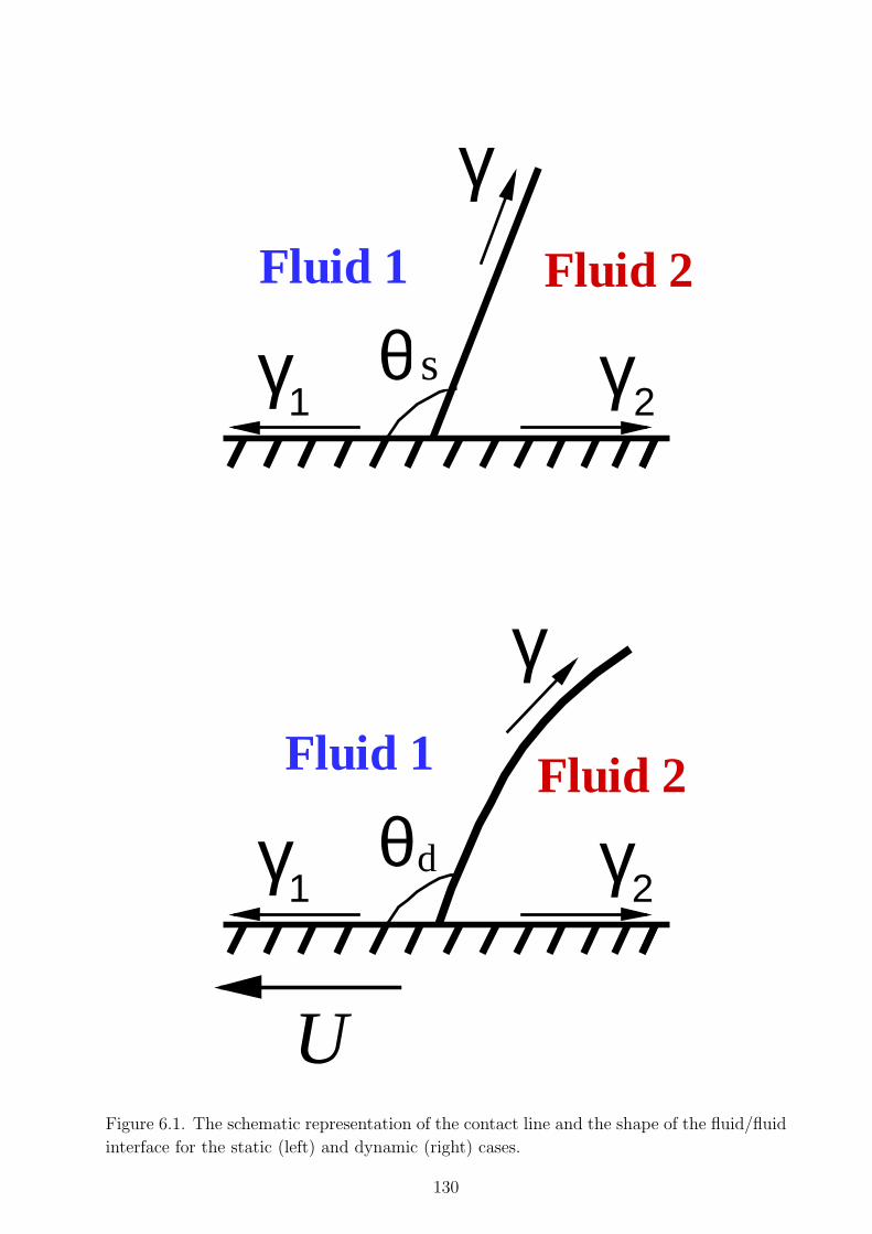
γ

γγ1 2

Fluid 1 Fluid 2

θs

γ

γγ1 2

Fluid 1 Fluid 2

θd

UFigure 6.1. The schematic representation of the contact line and the shape of the fluid/fluid

interface for the static (left) and dynamic (right) cases.

130

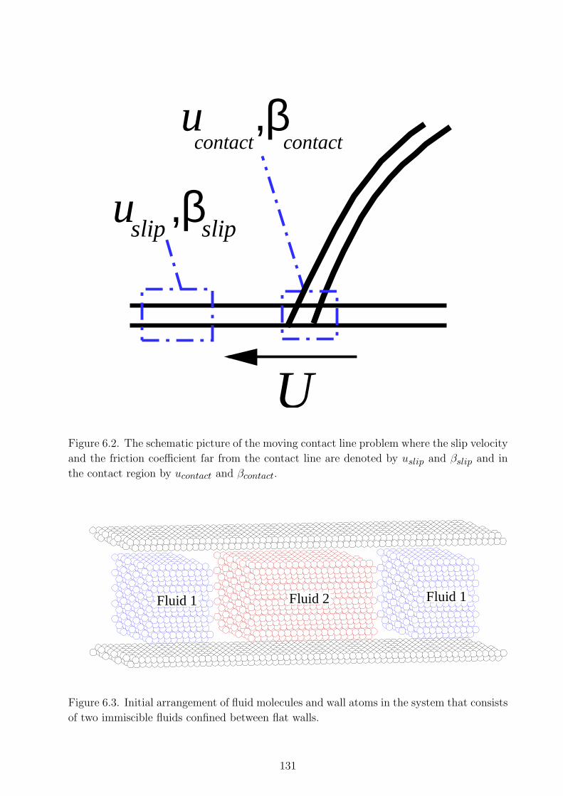
U

u

u

,β

,βslip

contact

slip

contact

Figure 6.2. The schematic picture of the moving contact line problem where the slip velocity

and the friction coefficient far from the contact line are denoted by uslip and βslip and in

the contact region by ucontact and βcontact.

Fluid 1 Fluid 1Fluid 2

Figure 6.3. Initial arrangement of fluid molecules and wall atoms in the system that consists

of two immiscible fluids confined between flat walls.

131

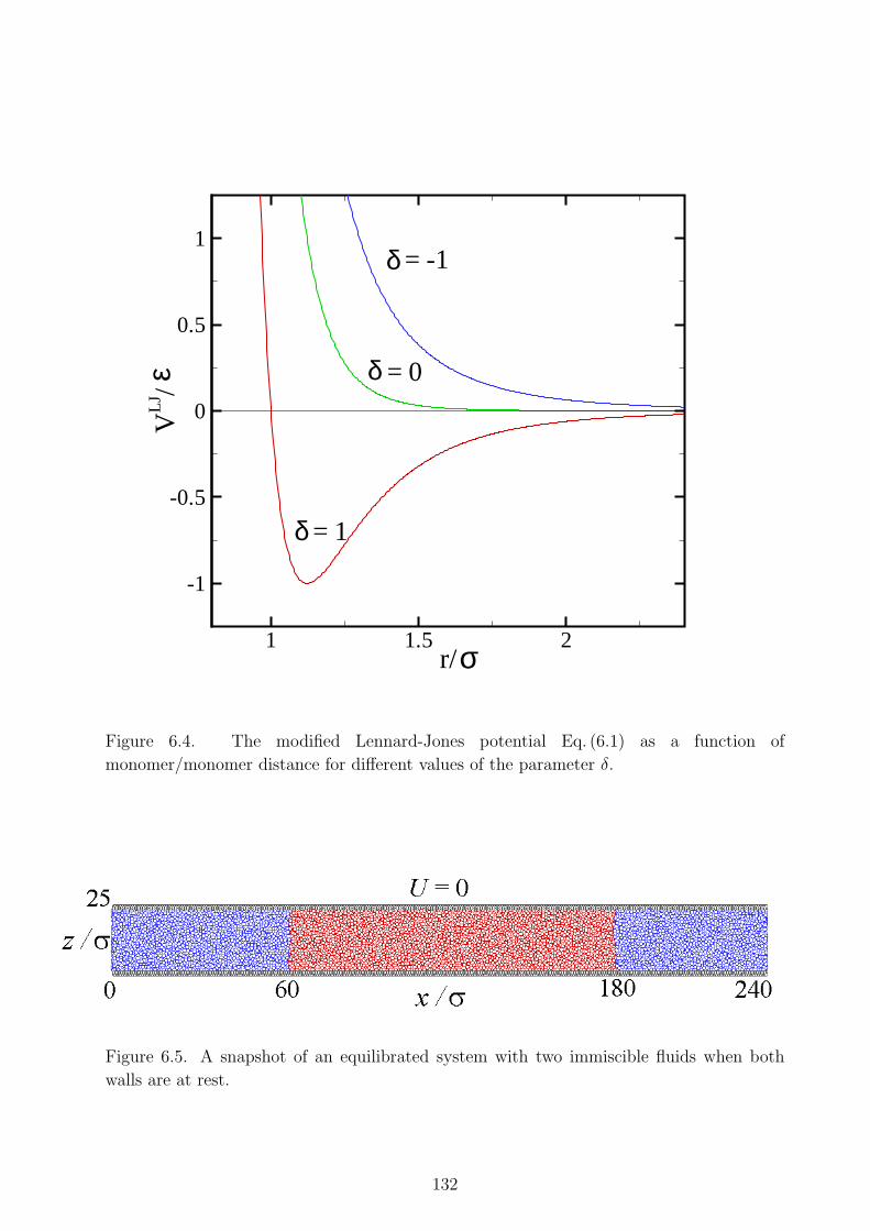
r/

VLJ

/

1 1.5 2

-1

-0.5

0

0.5

1

σ

ε

δ

δ

δ

= 1

= -1

= 0

Figure 6.4. The modified Lennard-Jones potential Eq. (6.1) as a function of

monomer/monomer distance for different values of the parameter δ.

Figure 6.5. A snapshot of an equilibrated system with two immiscible fluids when both

walls are at rest.

132

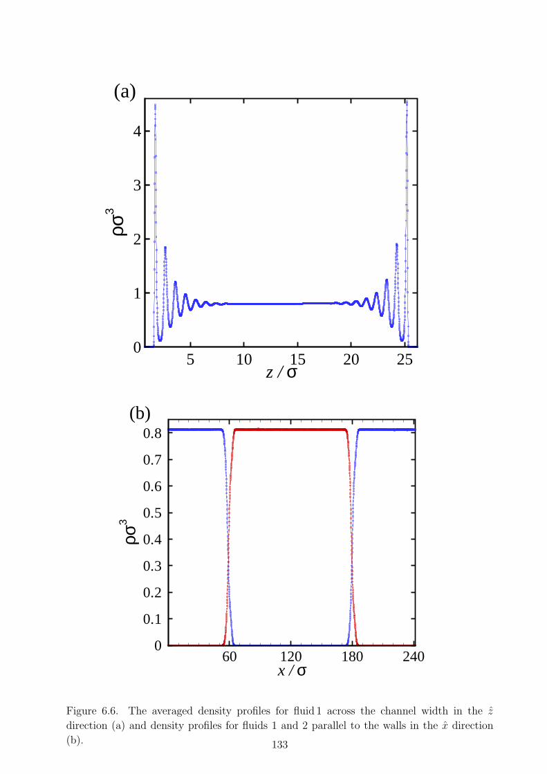
ρσ3

5 10 15 20 250

1

2

3

4

(a)

z / σ

ρσ3

60 120 180 2400

0.1

0.2

0.3

0.4

0.5

0.6

0.7

0.8

x / σ

(b)

Figure 6.6. The averaged density profiles for fluid 1 across the channel width in the z

direction (a) and density profiles for fluids 1 and 2 parallel to the walls in the x direction

(b). 133

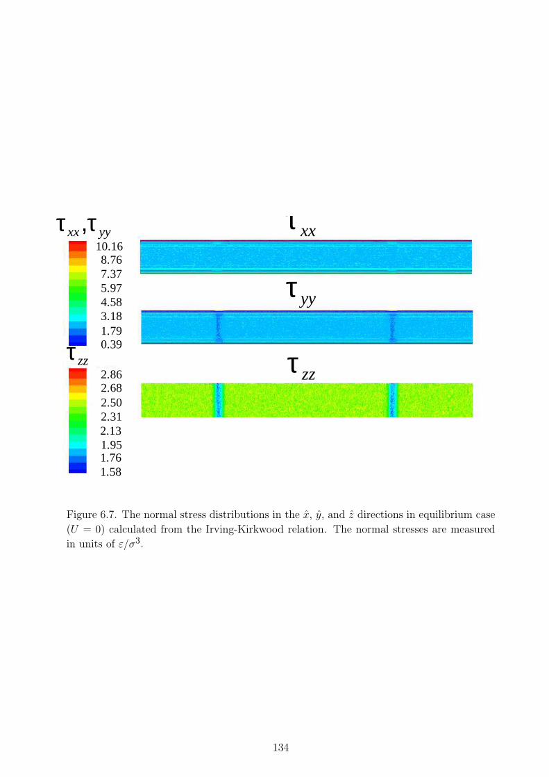
1.58

0.39

2.682.502.312.131.951.76

2.86

10.168.767.375.974.583.181.79

τ zz

,τ yy

τ yy

τ xx

τ zz

τ xx

Figure 6.7. The normal stress distributions in the x, y, and z directions in equilibrium case

(U = 0) calculated from the Irving-Kirkwood relation. The normal stresses are measured

in units of ε/σ3.

134

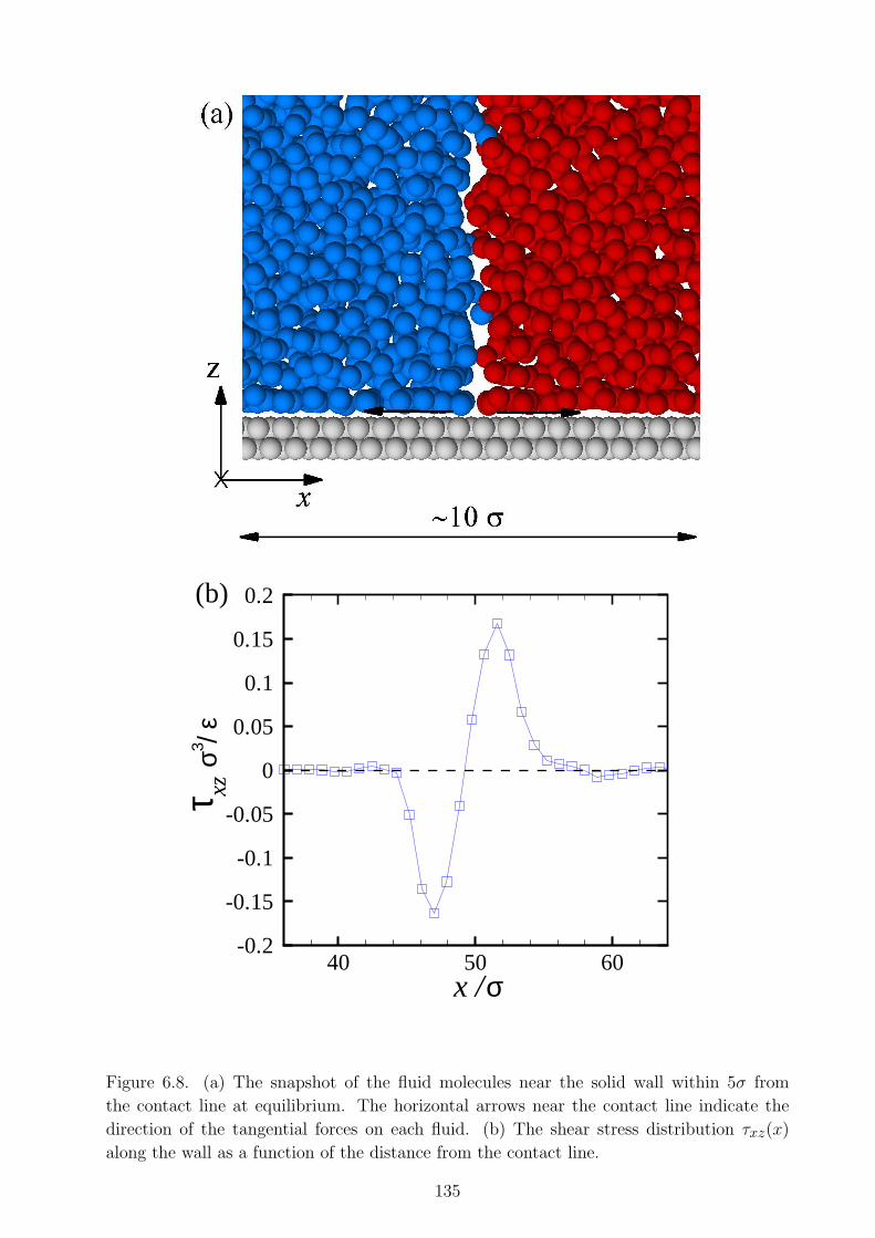
40 50 60-0.2

-0.15

-0.1

-0.05

0

0.05

0.1

0.15

0.2

x /σ

xz

(b)

σ3 /ετ

Figure 6.8. (a) The snapshot of the fluid molecules near the solid wall within 5σ from

the contact line at equilibrium. The horizontal arrows near the contact line indicate the

direction of the tangential forces on each fluid. (b) The shear stress distribution τxz(x)

along the wall as a function of the distance from the contact line.

135

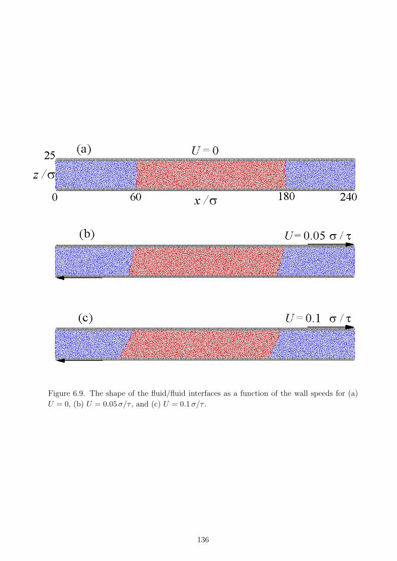
Figure 6.9. The shape of the fluid/fluid interfaces as a function of the wall speeds for (a)

U = 0, (b) U = 0.05 σ/τ , and (c) U = 0.1 σ/τ .

136

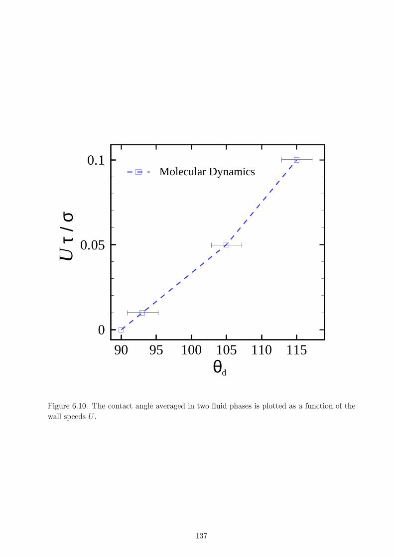
90 95 100 105 110 115

0

0.05

0.1

θ

U

d

Molecular Dynamics

τ/σ

Figure 6.10. The contact angle averaged in two fluid phases is plotted as a function of the

wall speeds U .

137

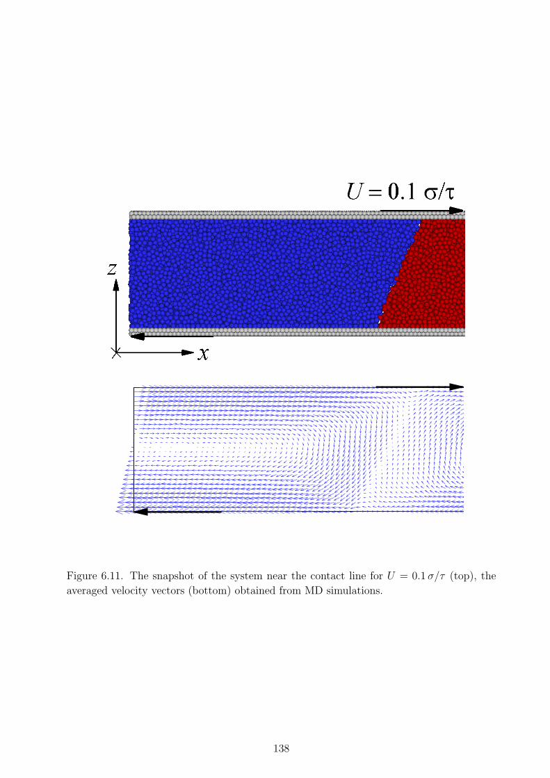
Figure 6.11. The snapshot of the system near the contact line for U = 0.1 σ/τ (top), the

averaged velocity vectors (bottom) obtained from MD simulations.

138

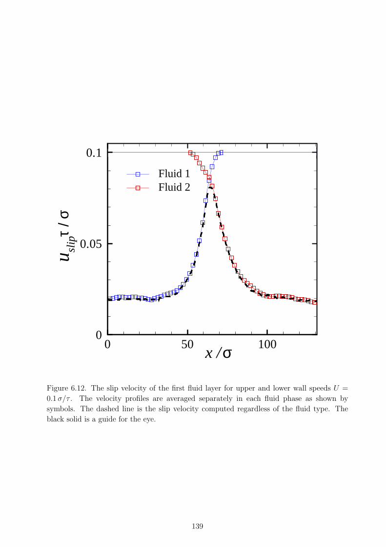
0 50 1000

0.05

0.1

x /σ

u slipτ/

σ

Fluid 1Fluid 2

Figure 6.12. The slip velocity of the first fluid layer for upper and lower wall speeds U =

0.1 σ/τ . The velocity profiles are averaged separately in each fluid phase as shown by

symbols. The dashed line is the slip velocity computed regardless of the fluid type. The

black solid is a guide for the eye.

139

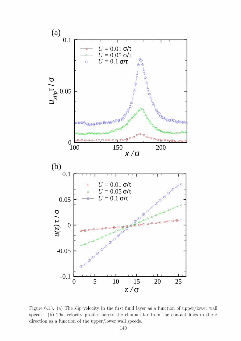
100 150 2000

0.05

0.1

x /σ

U = 0.1 σ/τ

U = 0.01 σ/τU = 0.05 σ/τ

u slip

(a)

τ/σ

0 5 10 15 20 25-0.1

-0.05

0

0.05

0.1

U = 0.1σ/τ

0.01U = σ/τU = 0.05σ/τ

z / σ

u(z)

(b)

τ/σ

Figure 6.13. (a) The slip velocity in the first fluid layer as a function of upper/lower wall

speeds. (b) The velocity profiles across the channel far from the contact lines in the z

direction as a function of the upper/lower wall speeds.

140

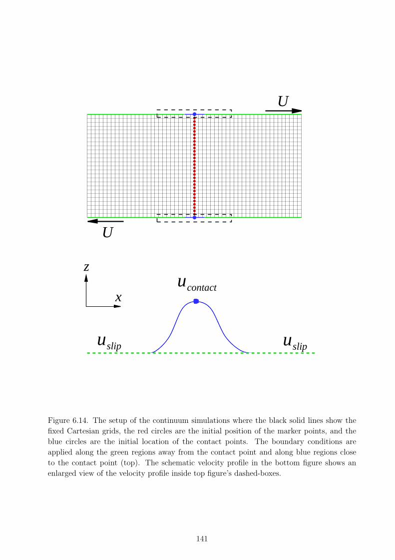
U

U

uslip

ucontact

uslip

x

z

Figure 6.14. The setup of the continuum simulations where the black solid lines show the

fixed Cartesian grids, the red circles are the initial position of the marker points, and the

blue circles are the initial location of the contact points. The boundary conditions are

applied along the green regions away from the contact point and along blue regions close

to the contact point (top). The schematic velocity profile in the bottom figure shows an

enlarged view of the velocity profile inside top figure’s dashed-boxes.

141

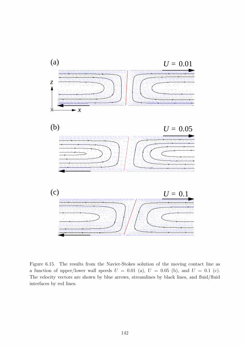
U = 0.01

x

z

(a)

U = 0.05(b)

U = 0.1(c)

Figure 6.15. The results from the Navier-Stokes solution of the moving contact line as

a function of upper/lower wall speeds U = 0.01 (a), U = 0.05 (b), and U = 0.1 (c).

The velocity vectors are shown by blue arrows, streamlines by black lines, and fluid/fluid

interfaces by red lines.

142

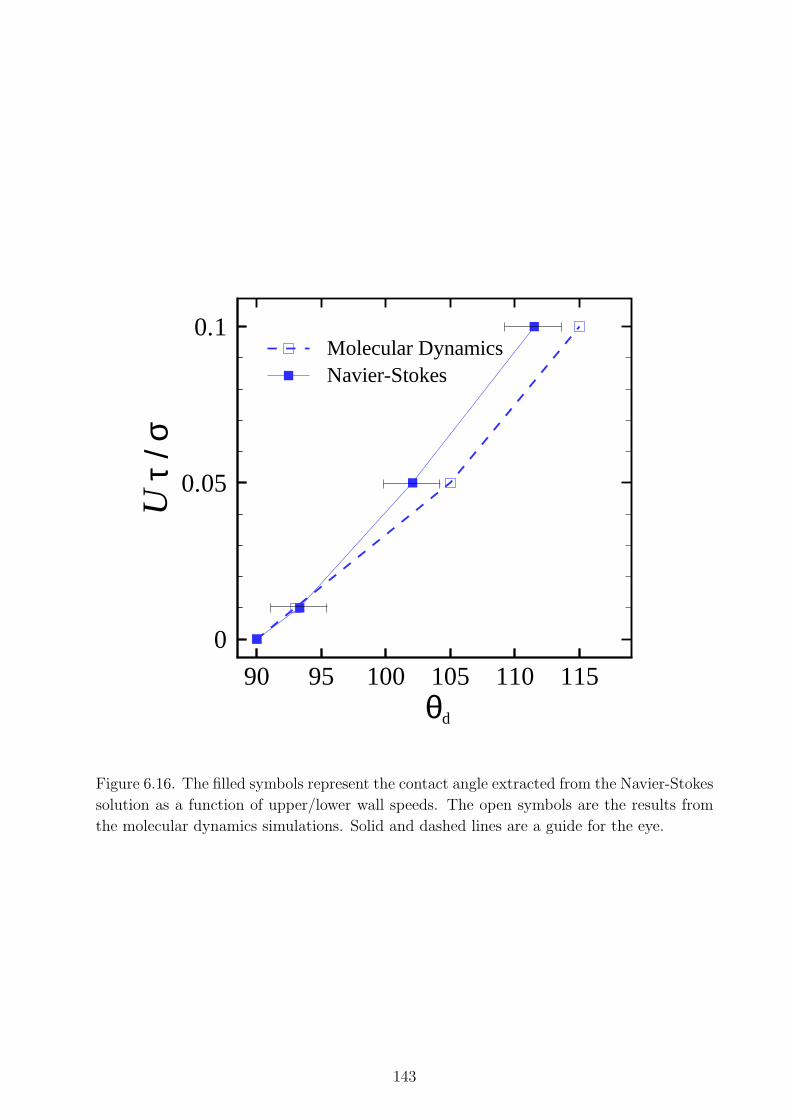
90 95 100 105 110 115

0

0.05

0.1

θ

U

d

Navier-StokesMolecular Dynamics

τ/σ

Figure 6.16. The filled symbols represent the contact angle extracted from the Navier-Stokes

solution as a function of upper/lower wall speeds. The open symbols are the results from

the molecular dynamics simulations. Solid and dashed lines are a guide for the eye.

143

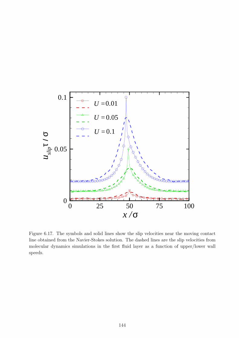
0 25 50 75 1000

0.05

0.1

0.1U =

U =

U =

0.01

0.05

x /σ

u slipτ/

σ

Figure 6.17. The symbols and solid lines show the slip velocities near the moving contact

line obtained from the Navier-Stokes solution. The dashed lines are the slip velocities from

molecular dynamics simulations in the first fluid layer as a function of upper/lower wall

speeds.

144

BIBLIOGRAPHY

145

[1] G. Karniadakis, A. Beskok, and N. Aluru, Microflows and nanoflows: Fundamentals

and simulation (Springer, New York, 2005).

[2] H. A. Stone, A. D. Stroock, and A. Ajdari, “Engineering flows in small devices: Mi-

crofluidics toward a lab-on-a-chip,” Annu. Rev. Fluid Mech. 36, 381 (2004).

[3] A. A. Darhuber and S. M. Troian, “Principles of microfluidic actuation by modulation

of surface stresses,” Annu. Rev. Fluid Mech. 37, 425 (2005).

[4] C. Neto, D. R. Evans, E. Bonaccurso, H. J. Butt, and V. S. J. Craig, “Boundary slip

in Newtonian liquids: A review of experimental studies,” Rep. Prog. Phys. 68, 2859

(2005).

[5] N. V. Churaev, V. D. Sobolev, and A. N. Somov, “Slippage of liquids over lyophobic

solid-surfaces,” J. Colloid Interface Sci. 97, 574 (1984).

[6] C. Cottin-Bizonne, S. Jurine, J. Baudry, J. Crassous, F. Restagno, and E. Charlaix,

“Nanorheology: An investigation of the boundary condition at hydrophobic and hy-

drophilic interfaces,” Eur. Phys. J. E 9, 47 (2002).

[7] L. Joly, C. Ybert, and L. Bocquet, “Probing the nanohydrodynamics at liquid-solid

interfaces using thermal motion,” Phys. Rev. Lett. 96, 046101 (2006).

[8] T. Schmatko, H. Hervet, and L. Leger, “Friction and slip at simple fluid-solid interfaces:

The roles of the molecular shape and the solid-liquid interaction,” Phys. Rev. Lett. 94,

244501 (2005).

[9] R. Pit, H. Hervet, and L. Leger, “Direct experimental evidence of slip in hexadecane:

Solid interfaces,” Phys. Rev. Lett. 85, 980 (2000).

[10] Y. Zhu and S. Granick, “Limits of the hydrodynamic no-slip boundary condition,”

Phys. Rev. Lett. 88, 106102 (2002).

[11] E. Bonaccurso, H. J. Butt, and V. S. J. Craig, “Surface roughness and hydrodynamic

boundary slip of a newtonian fluid in a completely wetting system,” Phys. Rev. Lett.

90, 144501 (2003).

[12] J. Sanchez-Reyes and L. A. Archer, “Interfacial slip violations in polymer solutions:

Role of microscale surface roughness,” Langmuir 19, 3304 (2003).

[13] T. Schmatko, H. Hervet, and L. Leger, “Effect of nanometric-scale roughness on slip

at the wall of simple fluids,” Langmuir 22, 6843 (2006).

[14] O. I. Vinogradova and G. E. Yakubov, “Surface roughness and hydrodynamic boundary

conditions,” Phys. Rev. E 73, 045302(R) (2006).

[15] K. B. Migler, H. Hervet, and L. Leger, “Slip transition of a polymer melt under shear

stress,” Phys. Rev. Lett. 70, 287 (1993).

146

[16] R. G. Horn, O. I. Vinogradova, M. E. Mackay, and N. Phan-Thien, “Hydrodynamic

slippage inferred from thin film drainage measurements in a solution of nonadsorbing

polymer,” J. Chem. Phys. 112, 6424 (2000).

[17] Y. Zhu and S. Granick, “Rate-dependent slip of Newtonian liquid at smooth surfaces,”

Phys. Rev. Lett. 87, 096105 (2001).

[18] V. S. J. Craig, C. Neto, and D. R. M. Williams, “Shear-dependent boundary Slip in an

aqueous Newtonian liquid,” Phys. Rev. Lett. 87, 054504 (2001).

[19] C. H. Choi, K. J. A. Westin, and K. S. Breuer, “Apparent slip flows in hydrophilic and

hydrophobic microchannels,” Phys. Fluids 15, 2897 (2003).

[20] J. Koplik, J. R. Banavar, and J. F. Willemsen, “Molecular dynamics of fluid flow at

solid interfaces,” Phys. Fluids A 1, 781 (1989).

[21] P. A. Thompson and M. O. Robbins, “Shear flow near solids: Epitaxial order and flow

boundary conditions,” Phys. Rev. A 41, 6830 (1990).

[22] P. A. Thompson, M. O. Robbins, and G. S. Grest, “Structure and shear response in

nanometer thick films,” Israel Journal of Chemistry 35, 93 (1995).

[23] P. A. Thompson and S. M. Troian, “A general boundary condition for liquid flow at

solid surfaces,” Nature (London) 389, 360 (1997).

[24] A. Jabbarzadeh, J. D. Atkinson, and R. I. Tanner, “Wall slip in the molecular dynamics

simulation of thin films of hexadecane,” J. Chem. Phys. 110, 2612 (1999).

[25] J.-L. Barrat and L. Bocquet, “Large slip effect at a nonwetting fluid-solid interface,”

Phys. Rev. Lett. 82, 4671 (1999).

[26] M. Cieplak, J. Koplik, J. R. Banavar, “Boundary conditions at a fluid-solid interface,”

Phys. Rev. Lett. 86, 803 (2001).

[27] N. V. Priezjev and S. M. Troian, “Molecular origin and dynamic behavior of slip in

sheared polymer films,” Phys. Rev. Lett. 92, 018302 (2004).

[28] T. M. Galea and P. Attard, “Molecular dynamics study of the effect of atomic roughness

on the slip length at the fluid-solid boundary during shear flow,” Langmuir 20, 3477

(2004).

[29] N. V. Priezjev, “Rate-dependent slip boundary conditions for simple fluids,” Phys. Rev.

E 75, 051605 (2007).

[30] R. Khare, J. J. dePablo, and A. Yethiraj, “Rheology of confined polymer melt,” Macro-

molecules 29, 7910 (1996).

[31] A. Koike and M. Yoneya, “Chain length effects on frictional behavior of confined ul-

trathin films of linear alkanes under shear,” J. Phys. Chem. B 102, 3669 (1998).

147

[32] A. Niavarani and N. V. Priezjev, “Slip boundary conditions for shear flow of polymer

melts past atomically flat surfaces,” Phys. Rev. E 77, 041606 (2008).

[33] J. P. Gao, W. D. Luedtke, and U. Landman, “Structures, solvation forces and shear of

molecular films in a rough nano-confinement,” Tribol. Lett. 9, 3 (2000).

[34] A. Jabbarzadeh, J. D. Atkinson, and R. I. Tanner, “Effect of the wall roughness on slip

and rheological properties of hexadecane in molecular dynamics simulation of Couette

shear flow between two sinusoidal walls,” Phys. Rev. E 61, 690 (2000).

[35] N. V. Priezjev and S. M. Troian, “Influence of periodic wall roughness on the slip

behaviour at liquid/solid interfaces: Molecular-scale simulations versus continuum pre-

dictions,” J. Fluid Mech. 554, 25 (2006).

[36] C. Kunert and J. Harting, “Roughness induced boundary slip in microchannel flows,”

Phys. Rev. Lett. 99, 176001 (2007).

[37] N. V. Priezjev, “Effect of surface roughness on rate-dependent slip in simple fluids,” J.

Chem. Phys. 127, 144708 (2007).

[38] E. Lauga and H. A. Stone, “Effective slip in pressure-driven Stokes flow,” J. Fluid

Mech. 489, 55 (2003).

[39] S. C. Hendy, M. Jasperse, and J. Burnell, “Effect of patterned slip on micro- and

nanofluidic flows,” Phys. Rev. E 72, 016303 (2005).

[40] N. V. Priezjev, A. A. Darhuber, and S. M. Troian, “Slip behavior in liquid films on

surfaces of patterned wettability: Comparison between continuum and molecular dy-

namics simulations,” Phys. Rev. E 71, 041608 (2005).

[41] T. Qian, X. P. Wang, and P. Sheng, “Hydrodynamic slip boundary condition at chem-

ically patterned surfaces: A continuum deduction from molecular dynamics,” Phys.

Rev. E 72, 022501 (2005).

[42] S. C. Hendy and N. J. Lund, “Effective slip boundary conditions for flows over nanoscale

chemical heterogeneities,” Phys. Rev. E 76, 066313 (2007).

[43] S. Richardson, “On the no-slip boundary condition,” J. Fluid Mech. 59, 707 (1973).

[44] C. Cottin-Bizonne, J.-L. Barrat, L. Bocquet, and E. Charlaix, “Low-friction flows of

liquid at nanopatterned interfaces,” Nature Mat. 2, 237 (2003).

[45] C. Cottin-Bizonne, C. Barentin, E. Charlaix, L. Bocquet, and J.-L. Barrat, “Dynam-

ics of simple liquids at heterogeneous surfaces: Molecular-dynamics simulations and

hydrodynamic description,” Eur. Phys. J. E 15, 427 (2004).

[46] M. Sbragaglia, R. Benzi, L. Biferale, S. Succi, and F. Toschi, “Surface roughness-

hydrophobicity coupling in microchannel and nanochannel flows,” Phys. Rev. Lett. 97,

204503 (2006).

148

[47] M. Sbragaglia and A. Prosperetti, “A note on the effective slip properties for microchan-

nel flows with ultrahydrophobic surfaces,” Phys. Fluids 19, 043603 (2007).

[48] J. Ou, B. Perot, and J. P. Rothstein, “Laminar drag reduction in microchannels using

ultrahydrophobic surfaces,” Phys. Fluids 16, 4635 (2004).

[49] C. H. Choi and C. J. Kim, “Large slip of aqueous liquid flow over a nanoengineered

superhydrophobic surface,” Phys. Rev. Lett. 96, 066001 (2006).

[50] P. Joseph, C. Cottin-Bizonne, J.-M. Benoit, C. Ybert, C. Journet, P. Tabeling, and

L. Bocquet, “Slippage of water past superhydrophobic carbon nanotube forests in mi-

crochannels,” Phys. Rev. Lett. 97, 156104 (2006).

[51] D. Einzel, P. Panzer, and M. Liu, “Boundary condition for fluid flow: Curved or rough

surfaces,” Phys. Rev. Lett. 64, 2269 (1990).

[52] P. Panzer, M. Liu, and D. Einzel, “The effects of boundary curvature on hydrodynamic

fluid flow: Calculation of slip lengths,” Int. J. Mod. Phys. B 6, 3251 (1992)

[53] K. Kremer and G. S. Grest, “Dynamics of entangled linear polymer melts: A molecular

dynamics simulation,” J. Chem. Phys. 92, 5057 (1990).

[54] G. S. Grest and K. Kremer, “Molecular-dynamics simulation for polymers in the pres-

ence of a heat bath,” Phys. Rev. A 33, 3628 (1986).

[55] J. P. Boon and S. Yip, Molecular Hydrodynamics (McGraw-Hill, New York, 1980).

[56] M. P. Allen and D. J. Tildesley, Computer Simulation of Liquids (Clarendon, Oxford,

1987).

[57] J. C. Heinrich and D. W. Pepper, Intermediate Finite Element Method: Fluid Flow

and Heat Transfer Applications (Taylor and Francis, Philadelphia, 1999).

[58] J. H. Irving and J. G. Kirkwood, “The statistical mechanical theory of transport

processes. IV. The equations of hydrodynamics,” J. Chem. Phys. 18, 817 (1950).

[59] R. B. Bird, C. F. Curtiss, R. C. Armstrong, and O. Hassager, Dynamics of Polymeric

Liquids 2nd ed. (Wiley, New York, 1987).

[60] Z. Xu, J. J. dePablo, and S. Kim, “Transport properties of polymer melts from non-

equilibrium molecular dynamics,” J. Chem. Phys. 102, 5836 (1995).

[61] J. T. Bosko, B. D. Todd, and R. J. Sadus, “Viscoelastic properties of denrimers in the

melt from nonequilibrium molecular dynamics,” J. Chem. Phys. 121, 12050 (2004).

[62] L. M. Hocking, “A moving fluid interface on a rough surface,” J. Fluid Mech. 76, 801

(1976).

[63] E. O. Tuck and A. Kouzoubov, “A laminar roughness boundary condition,” J. Fluid

Mech. 300, 59 (1995).

149

[64] T. Aoyagi, J. Takimoto, and M. Doi, “Molecular study of polymer melt confined be-

tween walls,” J. Chem. Phys. 115, 552 (2001).

[65] I. Bitsanis and G. Hadziioannou, “Molecular-dynamics simulations of the structure and

dynamics of confined polymer melts,” J. Chem. Phys. 92, 3827 (1990).

[66] S. J. Plimpton, J. Comp. Phys. 117, 1 (1995); see also URL http://lammps.sandia.gov.

[67] L. Bocquet and J.-L. Barrat, “Flow boundary conditions from nano- to micro-scales,”

Soft Matter 3, 685 (2007).

[68] V. Mhetar and L. A. Archer, “Slip in entangled polymer solutions,” Macromolecules

31, 6639 (1998).

[69] K. M. Awati, Y. Park, E. Weisser, and M. E. Mackay, “Wall slip and shear stresses

of polymer melts at high shear rates without pressure and viscous heating effects,” J.

Non-Newton. Fluid Mech. 89, 117 (2000).

[70] X. Zhou, D. Andrienko, L. Delle Site, and K. Kremer, “Flow boundary conditions for

chain-end adsorbing polymer blends,” J. Chem. Phys. 123, 104904 (2005).

[71] C. Pastorino, K. Binder, T. Kreer, and M. Muller, “Static and dynamic properties of

the interface between a polymer brush and a melt of identical chains,” J. Chem. Phys.

124, 064902 (2006).

[72] S. Barsky and M. O. Robbins, “Molecular dynamics study of slip at the interface

between immiscible polymers,” Phys. Rev. E 63, 021801 (2001).

[73] M. Tsige and G. S. Grest, “Molecular dynamics simulation of solventpolymer interdif-

fusion: Fickian diffusion,” J. Chem. Phys. 120, 2989 (2004).

[74] J. L. Barrat and J. P. Hansen, Basic concepts for simple and complex liquids (Cambridge

University Press, Cambridge, 2003).

[75] J. N. Israelachvili, Intermolecular and Surface Forces, 2nd ed. (Academic Press, San

Diego, 1992).

[76] M. O. Robbins, “Fluid dynamics: All stressed out,” Nature (London) 389, 331 (1997).

[77] Z. Xu, R. Khare, J. J. dePablo, and S. Kim, “On the calculation of transport properties

of polymer melts from nonequilibrium molecular dynamics,” J. Chem. Phys. 106, 8285

(1997).

[78] E. D. Smith, M. O. Robbins, and M. Cieplak, “Friction on adsorbed monolayers,” Phys.

Rev. B 54, 8252 (1996).

[79] M. S. Tomassone, J. B. Sokoloff, A. Widom, J. Krim, “Dominance of phonon friction

for a xenon film an a silver (111) surface,” Phys. Rev. Lett. 79, 4798 (1997).

[80] C. Pastorino, T. Kreer, M. Muller, and K. Binder, “Comparison of dissipative particle

dynamics and Langevin thermostats for out-of-equilibrium simulations of polymeric

systems,” Phys. Rev. E 76, 026706 (2007).

150

[81] D. J. Beebe, G. A. Mensing, and G. M. Walker, “Physics and applications of microflu-

idics in biology,” Annu. Rev. Biomed. Eng. 4, 261 (2002).

[82] T. M. Squires and S. R. Quake, “Microfluidics: Fluid physics at the nanoliter scale,”

Rev. Mod. Phys. 77, 977 (2005).

[83] V. Mengeaud, J. Josserand, and H. H. Girault, “Mixing processes in a zigzag microchan-

nel: Finite element simulations and optical study,” Anal. Chem. 74, 4279 (2002).

[84] A. Gigras and S. Pushpavanam, “Early induction of secondary vortices for micromixing

enhancement,” Microfluid. Nanofluid. 5, 89 (2008).

[85] H. M. Metwally and R. M. Manglik, “Enhanced heat transfer due to curvature-induced

lateral vortices in laminar flows in sinusoidal corrugated-plate channels,” Int. J. Heat

Mass Transfer 47, 2283 (2004).

[86] P. E. Geyer, N. R. Rosaguti, D. F. Fletcher, and B. S. Haynes, “Thermohydraulics

of square-section microchannels following a serpentine path,” Microfluid. Nanofluid. 2,

195 (2006).

[87] N. R. Rosaguti, D. F. Fletcher, and B. S. Haynes, “Low-Reynolds number heat transfer

enhancement in sinusoidal channels,” Chem. Eng. Sci. 62, 694 (2007).

[88] J. H. Forrester and D. F. Young, “Flow through a converging-diverging tube and its

implications in occlusive vascular disease. 1. Theoretical development,” J. Biomech. 3,

297 (1970).

[89] D. M. Wootton and D. N. Ku, “Fluid mechanics of vascular systems, diseases, and

thrombosis,” Annu. Rev. Biomed. Eng. 1, 299 (1999).

[90] S. A. Berger and L. D. Jou, “Flows in stenotic vessels,” Annu. Rev. Fluid Mech. 32,

347 (2000).

[91] C. Cottin-Bizonne, B. Cross, A. Steinberger, and E. Charlaix, “Boundary slip on

smooth hydrophobic surfaces: Intrinsic effects and possible artifacts,” Phys. Rev. Lett.

94, 056102 (2005).

[92] V. P. Sokhan, D. Nicholson, and N. Quirke, “Fluid flow in nanopores: An examination

of hydrodynamic boundary conditions,” J. Chem. Phys. 115, 3878 (2001).

[93] A. Niavarani and N. V. Priezjev, “Rheological study of polymer flow past rough surfaces

with slip boundary conditions,” J. Chem. Phys. 129, 144902 (2008).

[94] K. M. Jansons, “Determination of the macroscopic (partial) slip boundary condition for

a viscous flow over a randomly rough surface with a perfect slip microscopic boundary

condition,” Phys. Fluids 31, 15 (1988).

[95] M. J. Miksis and S. H. Davis, “Slip over rough and coated surfaces,” J. Fluid Mech.

273, 125 (1994).

151

[96] K. Sarkar and A. Prosperetti, “Effective boundary conditions for Stokes flow over a

rough surface,” J. Fluid Mech. 316, 223 (1996).

[97] C. Y. Wang, “Flow over a surface with parallel grooves,” Phys. Fluids 15, 1114 (2003).

[98] N. Lecoq, R. Anthore, B. Cichocki, P. Szymczak, and F. Feuillebois, “Drag force on a

sphere moving towards a corrugated wall,” J. Fluid Mech. 513, 247 (2004).

[99] J. C. F. Chow and K. Soda, “Laminar flow in tubes with constriction,” Phys. Fluids

15, 1700 (1972).

[100] G. L. Bordner, “Nonlinear analysis of laminar boundary layer flow over a periodic

wavy surface,” Phys. Fluids 21, 1471 (1978).

[101] S. Taneda, “Visualization of separating Stokes flows,” J. Phys. Soc. Jpn. 46, 1935

(1979).

[102] I. Sobey, “On flow through furrowed channels. Part 1. Calculated flow patterns,” J.

Fluid Mech. 96, 1 (1980).

[103] T. Nishimura, Y. Ohori, and Y. Kawamura, “Flow characteristics in a channel with

symmetric wavy wall for steady flow,” J. Chem. Eng. Japan 17, 466 (1984).

[104] S. Tsangaris and D. Potamitis, “On laminar small Reynolds-number flow over wavy

walls,” Acta Mechanica 61, 109 (1986).

[105] G. Leneweit and D. Auerbach, “Detachment phenomena in low Reynolds number

flows through sinusoidally constricted tubes,” J. Fluid Mech. 387, 129 (1999).

[106] H. Zhou, R. J. Martinuzzi, R. E. Khayat, A. G. Straatman, and E. Abu-Ramadan,

“Influence of wall shape on vortex formation in modulated channel flow,” Phys. Fluids

15, 3114 (2003).

[107] C. Pozrikidis, “Creeping flow in two-dimensional channels,” J. Fluid Mech. 180, 495

(1987).

[108] M. Scholle, A. Wierschem, and N. Aksel, “Creeping films with vortices over strongly

undulated bottoms,” Acta Mechanica 168, 167 (2004).

[109] J. C. Heinrich and R. S. Marshall, “Viscous incompressible flow by a penalty function

finite element method,” Computers and Fluids 9, 73 (1981).

[110] T. J. R. Hughes, W. K. Liu, and A. Brooks, “Finite element analysis of incompressible

viscous flows by the penalty function formulation,” J. Comp. Phys. 30, 1 (1979).

[111] T. B. Benjamin, “Shearing flow over a wavy boundary,” J. Fluid Mech. 6, 161 (1959).

[112] F. Pan and A. Acrivos, “Steady flows in rectangular cavities,” J. Fluid Mech. 28, 643

(1967).

[113] H. K. Moffatt, “Viscous and resistive eddies near a sharp corner,” J. Fluid Mech. 18,

1 (1964).

152

[114] H. Schlichting and K. Gersten, Boundary-Layer Theory (Springer, Berlin, 2000).

[115] P. Koumoutsakos, “Multiscale flow simulations using particles,” Annu. Rev. Fluid

Mech. 37, 457 (2005).

[116] D. A. Nield and A. Bejan, Convection in Porous Media (Springer, New York, 2006).

[117] J. Baudry, E. Charlaix, A. Tonck, and D. Mazuyer, “Experimental evidence for a large

slip effect at a nonwetting fluid-solid interface,” Langmuir 17, 5232 (2001).

[118] Y. Zhu and S. Granick, “No-slip boundary condition switches to partial slip when

fluid contains surfactant,” Langmuir 18, 10058 (2002).

[119] U. Ulmanella and C.-M. Ho, “Molecular effects on boundary condition in mi-

cro/nanoliquid flows,” Phys. Fluids 20, 101512 (2008).

[120] U. Heinbuch and J. Fischer, “Liquid flow in pores: Slip, no-slip, or multilayer sticking,”

Phys. Rev. A 40, 1144 (1989).

[121] J.-L. Barrat and L. Bocquet, “Influence of wetting properties on hydrodynamic bound-

ary conditions at a fluid/solid interface,” Faraday Discuss. 112, 119 (1999).

[122] S. C. Yang and L. B. Fang, “Effect of surface roughness on slip flows in hydrophobic

and hydrophylic microcannels by molecular dynamics simulation,” Molecular Simula-

tion 31, 971 (2005).

[123] A. Martini, H. Y. Hsu, N. A. Patankar, and S. Lichter, “Slip at high shear rates,”

Phys. Rev. Lett. 100, 206001 (2008).

[124] N. V. Priezjev, “Shear rate threshold for the boundary slip in dense polymer films,”

Phys. Rev. E 80, 031608 (2009).

[125] S. T. O’Connell and P. A. Thompson, “Molecular dynamics-continuum hybrid com-

putations: A tool for studying complex fluid flows,” Phys. Rev. E 52, R5792 (1995).

[126] E. G. Flekkøy, G. Wagner, and J. Feder, “Hybrid model for combined particle and

continuum dynamics,” Europhys. Lett. 52, 271 (2000).

[127] X. B. Nie, S. Y. Chen, W. E, and M. O. Robbins, “A continuum and molecular

dynamics hybrid method for micro- and nano-fluid flow,” J. Fluid Mech. 500, 55 (2004).

[128] Q. Li and G.-W. He, “An atomistic-continuum hybrid simulation of fluid flows over

superhydrophobic surfaces,” Biomicrofluidics 3, 022409 (2009).

[129] X. B. Nie, S. Y. Chen, and M. O. Robbins, “Hybrid continuum-atomistic simulation

of singular corner flow,” Phys. Fluids 16, 3579 (2004).

[130] N. G. Hadjiconstantinou, “Hybrid atomistic-continuum formulations and the moving

contact-line problem,” J. Comput. Phys. 154, 245 (1999).

[131] W. Q. Ren and W. E, “Heterogeneous multiscale method for the modeling of complex

fluids and microfluidics,” J. Comput. Phys. 204, 1 (2005).

153

[132] A. Niavarani and N. V. Priezjev, “The effective slip length and vortex formation in

laminar flow over a rough surface,” Phys. Fluids 21, 052105 (2009).

[133] W. Shyy, H.S. Udaykumar, M. M. Rao, and R. W. Smith, Computational Fluid Dy-

namics with Moving Boundaries (Dover Publications, Inc., New York, 1996).

[134] G. de Gennes, “Wetting: Statics and dynamics,” Rev. Mod. Phys. 57, 827 (1985).

[135] A. L. Yarin, “Drop impact dynamics: Splashing, spreading, receding, bouncing,”

Annu. Rev. Fluid Mech. 38, 159 (2006).

[136] C. Huh and L. E. Scriven, “Hydrodynamic model of steady movement of a

solid/liquid/fluid contact line,” J. Colloid Interface Sci. 35, 85 (1971).

[137] E. B. Dussan V., “On the spreading of liquids on solid surfaces: Static and dynamic

contact lines,” Annu. Rev. Fluid Mech. 11, 371 (1979).

[138] R. G. Cox, “The dynamics of the spreading of liquids on a solid surface. Part 1.

Viscous flow,” J. Fluid Mech. 168, 169 (1986).

[139] J. Koplik, J. R. Banavar, and J. F. Willemsen, “Molecular dynamics of Poiseuille flow

and moving contact lines,” Phys. Rev. Lett. 60, 1282 (1988).

[140] P. A. Thompson and M. O. Robbins, “Simulations of contact-line motion: Slip and

the dynamic contact angle,” Phys. Rev. Lett. 63, 766 (1989).

[141] P. A. Thompson, W. B. Brinckerhoff and M. O. Robbins, “Microscopic studies of

static and dynamic contact angles,” J. Adhesion Science and Technology 7, 535 (1993).

[142] N. G. Hadjicostantinou, “Combining atomistic and continuum simulations of contact-

line motion,” Phys. Rev. E 59, 2475 (1999).

[143] T. Qian, X. P. Wang, and P. Sheng, “Molecular scale contact line hydrodynamics of

immiscible flows,” Phys. Rev. E 68, 016306 (2003).

[144] W. Ren and W. E, “Boundary conditions for the moving contact line problem,” Phys.

Fluids 19, 022101 (2007).

[145] T. Ito, Y. Hirata, and Y. Kukita, “Fluid epitaxialization effect on velocity dependence

of dynamic contact angle on molecular scale,” J. Chem. Phys. 132, 054702 (2010).

[146] A. Niavarani and N. V. Priezjev, “Modeling the combined effect of surface roughness

and shear rate on slip flow of simple fluids,” Phys. Rev. E 81, 011606 (2010).

[147] C. Denniston and M. O. Robbins, “Mapping molecular models to continuum theories

for partially miscible fluids,” Phys. Rev. E 69, 021505 (2004).

[148] C. S. Peskin, “Numerical analysis of blood flow in the heart,” J. Comput. Phys. 25,

220 (1977).

154

[149] M. Griebel, T. Dornseifer, and T. Neunhoeffer, Numerical simulation in fluid dynam-

ics: A practical introduction (Society for industrial and applied mathematics, Philadel-

phia, 1998).

[150] W. Shyy, M. Francois, H. Udaykumar, N. N’dri, and R. Tran-son-tay, “Moving bound-

aries in micro-scale biofluid dynamics,” Appl. Mech. Rev. 54, 405 (2001).

155