MOISTURE CONTROL METHODOLOGY FOR GAS PHASE …

University of Kentucky University of Kentucky

UKnowledge UKnowledge

Theses and Dissertations--Biosystems and Agricultural Engineering Biosystems and Agricultural Engineering

2011

MOISTURE CONTROL METHODOLOGY FOR GAS PHASE MOISTURE CONTROL METHODOLOGY FOR GAS PHASE

COMPOST BIOFILTERS COMPOST BIOFILTERS

Lucas Dutra de Melo University of Kentucky, [email protected]

Right click to open a feedback form in a new tab to let us know how this document benefits you. Right click to open a feedback form in a new tab to let us know how this document benefits you.

Recommended Citation Recommended Citation Dutra de Melo, Lucas, "MOISTURE CONTROL METHODOLOGY FOR GAS PHASE COMPOST BIOFILTERS" (2011). Theses and Dissertations--Biosystems and Agricultural Engineering. 2. https://uknowledge.uky.edu/bae_etds/2

This Master's Thesis is brought to you for free and open access by the Biosystems and Agricultural Engineering at UKnowledge. It has been accepted for inclusion in Theses and Dissertations--Biosystems and Agricultural Engineering by an authorized administrator of UKnowledge. For more information, please contact [email protected].

http://uknowledge.uky.edu/

http://uknowledge.uky.edu/

https://uknowledge.uky.edu/

https://uknowledge.uky.edu/bae_etds

https://uknowledge.uky.edu/bae_etds

https://uknowledge.uky.edu/bae

https://uky.az1.qualtrics.com/jfe/form/SV_9mq8fx2GnONRfz7

mailto:[email protected]

STUDENT AGREEMENT: STUDENT AGREEMENT:

I represent that my thesis or dissertation and abstract are my original work. Proper attribution

has been given to all outside sources. I understand that I am solely responsible for obtaining

any needed copyright permissions. I have obtained and attached hereto needed written

permission statements(s) from the owner(s) of each third-party copyrighted matter to be

included in my work, allowing electronic distribution (if such use is not permitted by the fair use

doctrine).

I hereby grant to The University of Kentucky and its agents the non-exclusive license to archive

and make accessible my work in whole or in part in all forms of media, now or hereafter known.

I agree that the document mentioned above may be made available immediately for worldwide

access unless a preapproved embargo applies.

I retain all other ownership rights to the copyright of my work. I also retain the right to use in

future works (such as articles or books) all or part of my work. I understand that I am free to

register the copyright to my work.

REVIEW, APPROVAL AND ACCEPTANCE REVIEW, APPROVAL AND ACCEPTANCE

The document mentioned above has been reviewed and accepted by the student’s advisor, on

behalf of the advisory committee, and by the Director of Graduate Studies (DGS), on behalf of

the program; we verify that this is the final, approved version of the student’s dissertation

including all changes required by the advisory committee. The undersigned agree to abide by

the statements above.

Lucas Dutra de Melo, Student

Dr. George B. Day V, Major Professor

Dr. Dwayne Edwards, Director of Graduate Studies

MOISTURE CONTROL METHODOLOGY FOR GAS PHASE COMPOST

BIOFILTERS

THESIS

Master of Science in Biosystems and Agricultural Engineering in the College of Engineering at the University of Kentucky

By

Lucas Dutra de Melo

Lexington, Kentucky

Director: Dr. George B. Day V, Research Specialist

Lexington, Kentucky

2011

Copyright© Lucas Dutra de Melo 2011

ABSTRACT OF THE THESIS


BIOFILTERS

Gas phase biofilters are used for controlling odors from animal facilities.

Some characteristics can affect their performance and moisture content is one

very important. A methodology for controlling and measuring moisture content is

required to optimize these systems. An experiment was conducted to determine

the appropriate placement of a set of soaker hoses 1.2 m in length for water

application. It was found that the soaker hose installed in the lower region of the

biofilter coupled with appropriate and timely application of water was able to

minimize drying of the compost. Thermal conductance proved to be a reliable

indicator for measuring the moisture content. Biofilters using the soaker hoses

together with the thermal conductance as a media moisture sensor were able to

maintain moisture content above 30% w.b. which provided sufficient water for

microbial activity and ammonia abatement. A characterization of the ammonia

and nitrous oxide concentrations was performed in order to compare the

behavior of the gases when water was applied versus no water addition. These

analyses revealed that the overall performance was not significantly different

between treatments. But a more detailed assessment inside the biofilter media is

performed; it is possible to identify different processes taking place.

KEYWORDS: Compost Biofilters, thermal conductance, ammonia

removal, nitrous oxide, moisture content.

Lucas Dutra de Melo


BIOFILTERS

By

Lucas Dutra de Melo

Dr. George B. Day V

Dr. Dwayne Edwards

DEDICATION

To my mother Cláudia for the love, support,

caring and patience when I wasn’t present. To

my father José Sergio who always motivated

me to be my best and for the inspiration on

working hard. To my sister Isis for the support

and advice on the hardest decisions. And to

God for giving me strength and illumination to

walk my path.

DEDICAÇÃO

Para minha mãe Cláudia, pelo amor, suporte,

carinho e paciência quando não estive

presente. Para o meu pai José Sergio que

sempre me motivou a ser o meu melhor e pela

inspiração de sempre trabalhar duro. Para

minha irmã Isis pelo apoio e conselhos nas

mais difíceis decisões. E a Deus por me dar

força e iluminação na minha jornada.

iii

ACKNOWLEDGMENTS

First I would like to thanks God for strength, wisdom and illumination to

pursue my dreams and to hold on for the opportunities that life putted in my path.

Then I want to thank my family for the love, support and always believing

in me. I know that they were with me all the time, in the good and the bad. I am

thankful for everything they have done for me, for the education, the inspiration

and guidance that helped me to be the person I am today.

I want to thank Dr. George Day who has been more than a mentor for me

during my staying in Lexington; he has supported me, believed in me and helped

me in the difficult times and not only in the work. He helped me become a better

engineer with wise insights and advices. He is and always will be a friend, a

member of my chosen family.

Thanks to Dr Taraba for helping me when most needed in my work and for

the advices and teaching towards my degree. I know that his professionalism and

friendship will be always remembered.

Thanks to the former chairman of the Biosystems and Agricultural

Engineering Department Dr. Shearer for supporting my work and for financial

support.

I also want to thank the other member of my committee Dr. Gates for

giving me the opportunity to come to Unite States and pursue my degree, and for

being such a good friend, mentor and for believing in my work. And special

thanks for him for travelling 6 hours across 3 states to be present throughout my

work and to give so much good advice.

A special thanks for Dr. Del Nero Maia for being of so much help during

the whole project, for the tutoring and for putting the hands to work when

necessary. And of course for the fun outside the department, for presenting me

to the Lexington life, for the political conversations that for many times got some

heat coming out of it but always fun.

Thanks to Lloyd Dunn and Burl Fannin for all the help with the biofilters

and for putting stuff together, for helping me find tools whenever I needed and for

being there when I most needed somebody to give me a hand.

iv

Thanks to Andy Watson, Enrique Alves, Rodrigo Baldo, Williams Ferreira

and many others who helped me handle the compost, carry it, mix it with water

and of course load the biofilters; I know it was not an easy job and that was really

exhausting.

I want to express my appreciation to James Worten at the Waste Water

Treatment Plant of Lexington, KY, who received us with arms wide open to get

some samples of sludge, which was very important to the accomplishment of this

work.

Thanks to Michael Sama for his great help and teaching on the principles

of capacitance which was very helpful during the project and for helping me with

the electronics in my project.

Also thanks to Tatiana Sales that even from far away was always

available to give ideas and solutions for anything I asked.

A very special thanks for these two girls Daniela Sarti and Ester Buiate, I

do not think there are enough words to describe how important they are to me,

they make my life much easier in Lexington, giving me support when needed and

being strong handed when necessary. Thank you very much you are both my

adopted sisters, and I will take you in my heart forever.

And thanks to all the friends I made here: Santosh, Igor, Gabi,

Shankshank, Quélen, Luis Gustavo, Ricardo, Maíra, Rodrigo, Tatiana, Rogério,

Flávio and so many others that were really special to me and that forever will be

in my heart.

I know there is a lot of people that are not mentioned here, but I want them

to know that I am really thankful to everyone that made part of my life, you are

responsible for making me the person I am today.

I want to acknowledge the financial supported provided by USDA/ARS

Cooperative State Research, NRI Air Quality Program. Without their support this

project could not be accomplished.

v

Agradecimentos

Primeiro gostaria de agradecer a Deus pela força, sabedoria e iluminação

para perseguir meus sonhos e a agarrar as oportunidades que a vida pois no

meu caminho.

E também eu quero agradecer a minha família pelo amor, suporte e por

sempre acreditar em mim. Eu sei que eles estavam comigo o tempo todo, nos

bons e maus. Eu sou muito agradecido por tudo que eles fizeram por mim, pela

educação, inspiração e pela orientação que me ajudou a ser a pessoa que sou

hoje.

Eu quero agradecer Dr. George Day, quem tem sido mais do que um

mentor para mim durante minha estadia em Lexington, ele tem me dado suporte,

acreditado em mim e me ajudado nos tempos difíceis e não apenas no trabalho.

Ele me ajudou a ser um engenheiro melhor com suas dicas e conselhos. Ele é e

sempre será um amigo, um membro da minha família escolhida.

Obrigado ao Dr. Taraba por ter me ajudado quando eu mais precisei no

meu trabalho e por todos os conselhos e ensinamentos em prol da minha

formação. Eu sei que seu profissionalismo e amizade serão para sempre

lembrados.

Obrigado ao ex chefe do Departamento de Engenharia Agrícola e de

Biosistemas Dr. Shearer pelo suporte ao meu trabalho e pelo apoio financeiro.

Eu também gostaria de agradecer o outro membro do meu comitê Dr.

Gates por ter me dado a oportunidade de vir aos Estados Unidos para

prosseguir com minha formação, e por ter sido um bom amigo, tutor e por

acreditar no meu trabalho. E um agradecimento especial por ele viajar 6 horas

por 3 estados para estar presente durante meu trabalho e dar vários bons

conselhos.

Um agradecimento especial para o Dr. Del Nero Maia por ter sido tão

prestativo durante todo o projeto, pela tutoria e por ter posto as mãos na obra

quando necessário. E claro por toda a diversão fora do departamento, por ter

apresentado a vida em Lexington, pelas discussões políticas que várias vezes

se tornaram um pouco quentes mas acima de tudo divertidas.

vi

Obrigado ao Lloyd Dunn e Burl Fannin por toda a ajuda com os biofiltros e

por juntar as peças do quebra-cabeça, por ajudar a achar as diversas

ferramentas sempre que eu precisava e por estarem sempre dispostos a ajudar

na hora que eu mais precisei de uma mão.

Obrigado a Andy Watson, Enrique Alves, Rodrigo Baldo, Williams Ferreira

e muitos outros que ajudaram a trabalhar com o compost, carregá-lo, misturá-lo

com água e claro à carregar os biofiltros. Eu sei que não era um trabalho fácil e

sim muito cansativo.

Eu quero expressar minha gratidão à James Worten da Estação de

Tratamento de Água Residuária de Lexington, KY, quem nos recebeu de braços

abertos para pegar amostras de lodo, que foi muito importante para a conclusão

desse trabalho.

Obrigado ao Michael Sama por sua grande ajuda e ensinamentos nos

princípios da capacitância, os quais foram de muita ajuda durante o projeto e

pela ajuda com as partes eletrônicas do projeto.

Também obrigado a Tatiana Sales que mesmo estando longe sempre se

fez disponível para dar idéias e soluções para qualquer coisa que eu

perguntasse.

Um obrigado muito especial para essas duas garotas Daniela Sarti e

Ester Buiate. Eu não acho que existam palavras suficientes para descrever quão

importante elas são para mim, elas fizeram minha vida muito mais fácil em

Lexington, me dando suporte quando precisei e puxando minha orelha quando

necessário. Muito obrigado, vocês duas são minhas irmãs adotadas e eu vou

levá-las para sempre no meu coração.

E obrigado a todos os amigos que fiz aqui: Santosh, Igor, Gabi,

Shankshank, Quélen, Luis Gustavo, Ricardo, Maíra, Rodrigo, Tatiana, Rogério,

Flávio e vários outros que foram muito especiais para mim e que estarão para

sempre no meu coração.

Eu sei que existem muitas pessoas que não foram mencionadas aqui,

mas eu quero que elas saibam que eu estou muito agradecido por todos que

vii

fizeram parte da minha vida, vocês são responsáveis por terem feito de mim

quem eu sou hoje.

Quero reconhecer o apoio financeiro provido pelo USDA/ARS

Cooperative State Research, NRI Air Quality Program. Suporte sem o qual esse

projeto não poderia ser concluído

viii

Table of Contents

ACKNOWLEDGMENTS ............................................................................ iii

Table of Contents .................................................................................... viii

List of Figures ............................................................................................xi

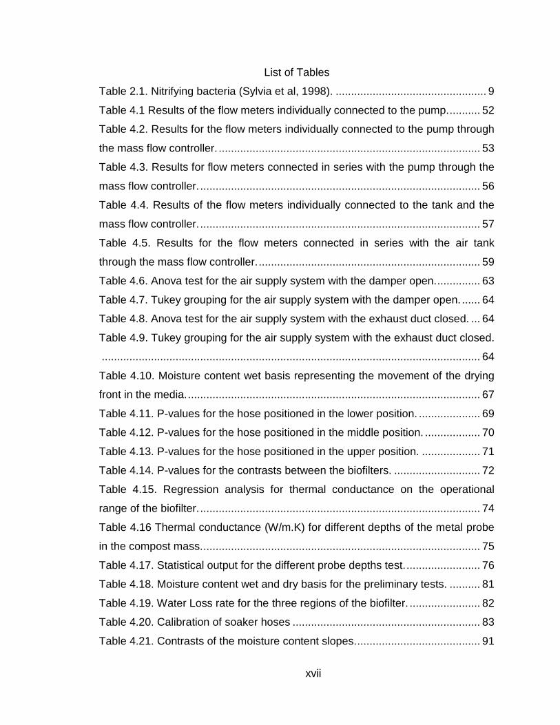
List of Tables .......................................................................................... xvii

Chapter 1 Introduction ............................................................................... 1

1.1 Summary .......................................................................................... 1

1.2 Justification ...................................................................................... 2

1.2.1 Importance ................................................................................. 2

1.3 Benefits ............................................................................................ 3

1.4 Objectives ........................................................................................ 3

1.5 Expected outcomes .......................................................................... 4

Chapter 2 Literature review ........................................................................ 5

2.1 Biofiltration ....................................................................................... 5

2.2 Compost ........................................................................................... 6

2.2.1 Porosity ...................................................................................... 6

2.2.2 Water Content ............................................................................ 7

2.2.3 Temperature .............................................................................. 7

2.2.4 Chemical Properties .................................................................. 8

2.2.5 Microbial population ................................................................... 9

2.3 Pilot Scale gas phase biofilters ........................................................ 9

2.4 Irrigation system ............................................................................. 10

2.5 Moisture sensing ............................................................................ 10

2.5.1 Capacitance technology .......................................................... 10

2.5.2 Thermal conductance technology ............................................ 10

ix

2.6 Gas sampling ................................................................................. 11

2.6.1 Manual ..................................................................................... 11

2.6.2 Automated ............................................................................... 12

Chapter 3 Material and Methods .............................................................. 13

3.1 Biofilters chambers ......................................................................... 13

3.1.1 Flow meter test ........................................................................ 15

3.1.2 Chamber leakage .................................................................... 17

3.1.3 Balancing the system: exhaust side ......................................... 20

3.1.4 Balancing the system: supply side ........................................... 21

3.2 Sieve shaker machine .................................................................... 23

3.3 Physical properties ......................................................................... 26

3.3.1 Particle size distribution ........................................................... 26

3.3.2 Compost water content ............................................................ 26

3.4 Irrigation system ............................................................................. 37

3.4.1 Calibration................................................................................ 38

3.4.2 Positioning Experiment ............................................................ 39

3.4.3 Water application interval ........................................................ 44

3.5 Ammonia and Nitrous Oxide observations ..................................... 45

3.5.1 Experimental set-up ................................................................. 45

3.5.2 Water balance .......................................................................... 48

3.5.3 Concentration analysis ............................................................ 49

Chapter 4 Results and discussion ........................................................... 51

4.1 The biofilter chambers ................................................................. 51

4.1.1 Flow meter test ...................................................................... 51

4.1.2 Chamber leakage .................................................................. 59

x

4.1.3 Balancing the system: exhaust side ...................................... 61

4.1.4 Balancing the system: supply system side ............................ 63

4.2 Sieve shaker machine ................................................................. 64

4.3 Physical properties ...................................................................... 65

4.3.1 Particle size distribution ......................................................... 65

4.3.2 Compost water content .......................................................... 66

4.4 Irrigation system .......................................................................... 78

4.4.1 Preliminary test and calibration ............................................. 78

4.4.2 Soaker hose test.................................................................... 82

4.4.3 Hose positioning (water added) ............................................. 84

4.4.4 Water application interval ...................................................... 91

4.5 Ammonia and Nitrous Oxide Observations .................................. 93

4.5.1 Water balance ....................................................................... 93

4.5.2 Ammonia Removal .............................................................. 109

4.5.3 Nitrous oxide ....................................................................... 124

Chapter 5 Conclusions........................................................................... 134

Chapter 6 Recommendations for future work ........................................ 138

Appendices ............................................................................................ 139

Appendix A.Evaluation of capacitance as moisture measure method

...................................................................................................................... 139

Appendix B. Statistical Analysis for Flow meters tests ..................... 160

Appendix C. Statistical Analysis for the drying front movement ....... 164

Appendix D. Nitrous Oxide Removal efficiencies Statistics .............. 170

Appendix E. Water replacement calculation..................................... 174

References ............................................................................................ 177

Vita......................................................................................................... 181

xi

List of Figures

Figure 2.1. Nitrogen Cycle (Sylvia et al, 1998) ..................................................... 6

Figure 2.2. From Del Nero Maia (2010), automated sampling system: control

diagram. ............................................................................................................. 12

Figure 3.1. Biofilter chambers in the Agriculture Air Quality Laboratory (Sales,

2008). ................................................................................................................. 14

Figure 3.2. Modifications of the biofilter chamber. .............................................. 15

Figure 3.3. Schematic for flow meter connections in series with both: air pump or

pressurized air cylinder. ...................................................................................... 16

Figure 3.4. Setup of the flow meters connected in series with the pump (not

shown) or the cylinder through the mass flow controller. .................................... 17

Figure 3.5. Smoke machine connected to the biofilter plenum ........................... 18

Figure 3.6. Smoke passing through the compost. .............................................. 19

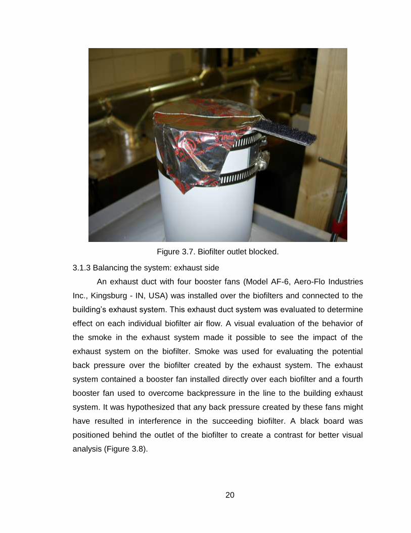
Figure 3.7. Biofilter outlet blocked. ..................................................................... 20

Figure 3.8. Black board positioned behind the outlet, with smoke coming out. .. 21

Figure 3.9. System connecting the fan to the plenum and biofilters. .................. 22

Figure 3.10. Air regulator and air delivery to the plenum. ................................... 22

Figure 3.11. Position of the measurements for air flow from the plenum. ........... 23

Figure 3.12. Sales (2008) sieving machine. ....................................................... 24

Figure 3.13. 3D model of the improved sieve shaker. ........................................ 25

Figure 3.14. Sieve shaker machine with the add-on component. ....................... 26

Figure 3.15. Biofilter and its regions. .................................................................. 29

Figure 3.16. Grabber tool. .................................................................................. 30

Figure 3.17. Side wall openings for the grabber tool. ......................................... 30

Figure 3.18. Grabbing tool for taking samples. ................................................... 31

Figure 3.19. Containers used for storage. .......................................................... 32

Figure 3.20. Concrete mixer used for mixing compost. ...................................... 33

Figure 3.21. Cups filled with compost at different moisture levels ...................... 34

Figure 3.22. Decagon probe inserted into the compost. ..................................... 35

Figure 3.23. Thermal conductance probe tested for plywood wall effect. ........... 36

xii

Figure 3.24. Thermal conductance measurement when the probe is inserted 1/3

of the length. ....................................................................................................... 37

Figure 3.25. Hose Calibration device. ................................................................. 38

Figure 3.26. Pressure gauge. ............................................................................. 39

Figure 3.27. Conical drying noted by Sales, 2008 .............................................. 40

Figure 3.28. Conical drying formation in the biofilters. ........................................ 41

Figure 3.29. Hose located in the lower position. ................................................. 42

Figure 3.30. Hose located in the middle position. ............................................... 42

Figure 3.31. Hose located at the upper position in the biofilter. .......................... 43

Figure 3.32. Container collecting water from the biofilter. ................................... 45

Figure 3.33. Multiplexer connecting the sampling points of the INNOVA. .......... 47

Figure 3.34. Solenoid valves within the multiplexer box. .................................... 47

Figure 3.35. INNOVA photoacoustic gas analyzer. ............................................ 48

Figure 4.1. Graph representing the flow meters connected individually with the

pump through the mass flow controller. .............................................................. 54

Figure 4.2. Graph representing the flow meters connected individually with the

pump through the mass flow controller in the range between 20 and 40 ml/min. 55

Figure 4.3. Graphic representing the flow meters connected to the tank

individually through the mass flow controller. ..................................................... 58

Figure 4.4. Smoke rising to the media surface. .................................................. 60

Figure 4.5. No back pressure over biofilter 1. ..................................................... 62

Figure 4.6. Slight back pressure over biofilter 2. ................................................. 62

Figure 4.7. Showing back pressure over biofilter 3. ............................................ 63

Figure 4.8. As received compost particle size distribution. ................................. 65

Figure 4.9. Characterization of the drying front movement in the biofilter. .......... 68

Figure 4.10. Drying pattern for lower region. ...................................................... 69

Figure 4.11. Drying pattern for middle region. .................................................... 70

Figure 4.12. Drying pattern for upper region. ...................................................... 71

Figure 4.13. Thermal conductance exponential regression for compost medium

particle sizes. ...................................................................................................... 72

xiii

Figure 4.14. Thermal conductance linear regression for compost medium particle

sizes. .................................................................................................................. 73

Figure 4.15. Preliminary test for water demand calculation. ............................... 79

Figure 4.16. Linear regression of the soaker hose flow with the pressure. ......... 83

Figure 4.17. Chart showing the moisture content of the regions of biofilters with

the hose installed in the lower position. .............................................................. 85

Figure 4.18. SAS output to the lower region when the hose is positioned in the

lower region. ....................................................................................................... 85

Figure 4.19. SAS output to the middle region when the hose is positioned in the

lower region. ....................................................................................................... 86

Figure 4.20. SAS output to the upper region when the hose is positioned in the

lower region. ....................................................................................................... 86


the hose installed in the middle position. ............................................................ 87

Figure 4.22. SAS output to the lower region when the hose is positioned in the

middle region. ..................................................................................................... 87


middle region. ..................................................................................................... 88


middle region. ..................................................................................................... 88


the hose installed in the middle position. ............................................................ 89

Figure 4.26. SAS output of the equilibrium period of the lower region when the

hose is positioned in the upper region. ............................................................... 89

Figure 4.27. SAS output of the middle region when the hose is positioned in the

upper region. ...................................................................................................... 90

Figure 4.28. SAS output of the upper region when the hose is positioned in the

upper region. ...................................................................................................... 90

Figure 4.29. Moisture content in the three regions of the biofilter during the run

when no water was applied. ............................................................................... 94

xiv

Figure 4.30. Moisture content in the three regions of the biofilter during the run

when water was applied according to the thermal conductance sensor. ............ 94

Figure 4.31. Lower region drying fronts comparison between the treatments with

no water and water applied. ............................................................................... 95

Figure 4.32. Middle region drying fronts comparison between the treatments with


Figure 4.33. Upper region drying fronts comparison between the treatments with


Figure 4.34. Water vapor profile in the biofilter. ................................................ 102

Figure 4.35. Water removed from the biofilter. ................................................. 104

Figure 4.36. Thermal conductance in the biofilter compost in the three regions.

......................................................................................................................... 105

Figure 4.37. SAS output for the thermal conductance readings after 250 hours.

......................................................................................................................... 105

Figure 4.38. Calculated moisture content based on the equation 4.1 calibrated for

thermal conductance. ....................................................................................... 106

Figure 4.39. Comparison of the moisture content calculated by the thermal

conductance method with the oven method at the lower position of the biofilters.

......................................................................................................................... 107


conductance method with the oven method at the middle position of the biofilters.

......................................................................................................................... 108



......................................................................................................................... 108

Figure 4.42. Ammonia removal efficiency for the lower region with no water. .. 109

Figure 4.43. Ammonia removal efficiency for the middle region with no water. 110

Figure 4.44. Ammonia removal efficiency for the upper region with no water. . 111

Figure 4.45. Ammonia removal efficiency for the headspace region with no water.

......................................................................................................................... 112

xv

Figure 4.46. Ammonia removal efficiency for the overall biofilter with no water.

......................................................................................................................... 112

Figure 4.47. Graphical representation of the moisture content and the ammonia

removal of the lower region during the treatment when no water is being added.

......................................................................................................................... 113



......................................................................................................................... 114



......................................................................................................................... 115

Figure 4.50. Ammonia removal efficiency for the lower region with water. ....... 116

Figure 4.51. Ammonia removal efficiency for the middle region with water. ..... 117

Figure 4.52. Ammonia removal efficiency for the upper region with water. ...... 118

Figure 4.53. Ammonia removal efficiency for the headspace region with water.

......................................................................................................................... 119

Figure 4.54. Ammonia removal efficiency for the overall biofilter with water. ... 120

Figure 4.55. Profile of moisture content during the test with water being applied.

......................................................................................................................... 121


removal of the lower region during the treatment with water being added. ....... 122


removal of the middle region during the treatment with water being added. ..... 123


removal of the upper region during the treatment with water being added. ...... 124

Figure 4.59. Nitrous oxide progression in the lower region with no water. ........ 125



Figure 4.62. Nitrous oxide progression in the headspace region with no water.

......................................................................................................................... 128

Figure 4.63. Nitrous oxide removal efficiency in the lower region with water. ... 129

xvi

Figure 4.64. Nitrous oxide removal efficiency in the middle region with water. . 130

Figure 4.65. Nitrous oxide removal efficiency in the upper region with water. .. 131

Figure 4.66. Nitrous oxide removal efficiency in the upper region with water. .. 132

Figure 4.67. Nitrous oxide removal efficiency in the overall biofilter with water. 133

xvii

List of Tables

Table 2.1. Nitrifying bacteria (Sylvia et al, 1998). ................................................. 9

Table 4.1 Results of the flow meters individually connected to the pump. .......... 52

Table 4.2. Results for the flow meters individually connected to the pump through

the mass flow controller. ..................................................................................... 53

Table 4.3. Results for flow meters connected in series with the pump through the

mass flow controller. ........................................................................................... 56

Table 4.4. Results of the flow meters individually connected to the tank and the

mass flow controller. ........................................................................................... 57

Table 4.5. Results for the flow meters connected in series with the air tank

through the mass flow controller. ........................................................................ 59

Table 4.6. Anova test for the air supply system with the damper open. .............. 63

Table 4.7. Tukey grouping for the air supply system with the damper open. ...... 64

Table 4.8. Anova test for the air supply system with the exhaust duct closed. ... 64

Table 4.9. Tukey grouping for the air supply system with the exhaust duct closed.

........................................................................................................................... 64

Table 4.10. Moisture content wet basis representing the movement of the drying

front in the media. ............................................................................................... 67

Table 4.11. P-values for the hose positioned in the lower position. .................... 69

Table 4.12. P-values for the hose positioned in the middle position. .................. 70

Table 4.13. P-values for the hose positioned in the upper position. ................... 71

Table 4.14. P-values for the contrasts between the biofilters. ............................ 72

Table 4.15. Regression analysis for thermal conductance on the operational

range of the biofilter. ........................................................................................... 74

Table 4.16 Thermal conductance (W/m.K) for different depths of the metal probe

in the compost mass. .......................................................................................... 75

Table 4.17. Statistical output for the different probe depths test. ........................ 76

Table 4.18. Moisture content wet and dry basis for the preliminary tests. .......... 81

Table 4.19. Water Loss rate for the three regions of the biofilter. ....................... 82

Table 4.20. Calibration of soaker hoses ............................................................. 83

Table 4.21. Contrasts of the moisture content slopes. ........................................ 91

xviii

Table 4.22. Water interval evaluation. ................................................................ 92

Table 4.23. Tukey grouping for water interval tests. ........................................... 92

Table 4.24. Mass of water lost in the biofilter when no water is applied into the

media. ................................................................................................................. 98

Table 4.25. Water loss for the biofilter when water is applied into the media. .. 100

Table 4.26. Water loss for the biofilter treatment for water applied into the media,

taking into consideration the water added during the process. ......................... 101

1

Chapter 1 Introduction

1.1 Summary

The emission of greenhouse gases (GHG’s) by confined animal feeding

operations (CAFO’s) has become an important issue as governments consider

the establishment of stricter limits on GHG emissions. Mitigation strategies are

being developed involving new and emerging technologies to reduce these

emissions. One technology to treat ventilation air that has been studied is the

compost-based biofilter because of its economy, ease of maintenance and

sustainability.

Compost-based biofilter performance depends on variables related to the

physical characteristics of the media. Considerable work has been accomplished

to define these characteristics and their effects on biofilter performance.

Research conducted by Sales (2008) identified an optimal media particle size

distribution which minimized the pressure drop across the media stack. Further, it

has been shown that moisture content is a key variable in maximizing biological

conversion of ammonia (NH3) to nitrate-N and ultimately to nitrogen gas (N2).

However, the importance of optimal media moisture content has only been

recently identified. Del Nero Maia (2010) has shown that the media moisture

content not only affected microbial activity that oxidizes ammonia, but recognized

some moisture content conditions that can work as a trigger for nitrous oxide

(N2O) and methane (CH4) production. Nitrous oxide (N2O) and methane are

greenhouse gases which exert a significant impact on the radiation heat balance

of the planet (Lashof, 1990).

Increased demand for food in the world has resulted in increased need

within the agri-business sector to supply more foodstuffs as efficiently as

possible. High density food production must necessarily involve increased

agriculture activity and often, these enterprises may involve higher production of

GHG’s. Thus, in order to meet world food demand, new and more efficient

techniques for mitigation of these gases are necessary. Previous work has

shown that biofilter efficiency is directly related to moisture content. Therefore, to

be considered efficient, a biofilter must include effective, reliable instrumentation

2

for media moisture control. The purpose of this work is to establish a system that

will deliver water to the media to maintain certain prescribed levels of moisture

content to maximize NH3 conversion and minimize or prevent N2O production.

1.2 Justification

1.2.1 Importance

Researchers worldwide are studying the effects of greenhouse gases on

climate change and it is known that agriculture contributes significantly to GHG

production. Specifically, livestock production generates various harmful gases

like methane and carbon dioxide; which have been targeted as chief contributors.

Increased food production in this case will lead to increased generation of

potentially harmful gases. The generation of GHG and its relation to climate

change continues to be an important topic of discussion and this relation has yet

to be proven. However solutions for mitigation of these gases have been

developed and are being placed on the market as a means to control the

increased amount of gas emitted into the atmosphere. Smith (2007) listed

various technologies such as cropland management, pasture improvement,

management of organic soils, restoration of degraded lands and livestock and

manure management which include biofiltration.

Biofiltration is an important mitigation technology which has been proven

cost-effective and environmentally friendly. Further, the biomass for the media

may be a waste by-product which figures as a sustainable method for waste

recycling. Operational strategies for biofilters to effectively mitigate the exhaust

gas(es) of concern continue to evolve as the science behind the reactions within

the biofilters is developed. Recent findings have shown that various

characteristics of the biomedia itself, such as moisture content (Del Nero Maia,

2010) and particle size (Sales, 2008) can affect biofilter performance and even

create conditions that can produce higher levels of harmful gases like nitrous

oxide. The media particle size can affect the performance through formation of

preferential flow pathways (Sales, 2008) and excessive moisture content in the

compost can create conditions that favor the transformation of ammonia into

3

nitrous oxide (Del Nero Maia, 2010) by affecting the particle micro-environment

oxygen concentrations and microbial viability on external surfaces and internal

pores. This latter consideration is of particular concern to researchers owing to

the nature of the gas itself. Nitrous oxide is considered to have the equivalent

global warming potential of approximately 180 units of CO2 in the atmosphere

(Lashof, 1990). Thus the need for an adequate moisture measurement and

delivery system is demonstrated. Accurate control of moisture will optimize the

process of biofiltration for maximum ammonia conversion and minimum nitrous

oxide production.

1.3 Benefits

Biofilters operating at optimal moisture levels should provide higher rates

of ammonia conversion and minimize nitrous oxide production. This system

coupled with its relatively low operating costs and high sustainability will provide

society with a tool to reduce the emission of greenhouse gases to the

atmosphere. This may in turn, reduce the impact of the animal production system

on climate change. In the short term this technology could provide society with a

cleaner exhaust air that lowers impacts on those individuals that live or work in

the surroundings of agricultural facilities and provide improved animal welfare

and a more comfortable place to work.

1.4 Objectives

The scope of this study is to evaluate and test an indirect method for

moisture measurement coupled with a method for applying water in gas phase

compost biofilters in order to maintain optimal moisture levels. The major

objectives of this work are:

Objective 1:

Evaluate the use of commercially available “soaker hoses” as a method

for moisture delivery and to determine the effect of vertical position within the

biofilter on moisture content uniformity.

4

Objective 2:

Evaluate the thermal conductance of the biofilter media as an indirect

means for moisture measurement.

Objective 3:

Determine the effect of the moisture control methodology on the ammonia

and nitrous oxide concentrations across the gas phased biofilter.

1.5 Expected outcomes

Objective 1:

An optimal vertical positioning of a set of commercially available soaker

hoses within the media does exist to maintain a set moisture level in the entire

biofilter volume.

Objective 2:

The relationship between the moisture content and the thermal

conductance, and to use this property as reference in a model for predicting

moisture content.

Objective 3:

The effect of the use of a uniform, controlled moisture application system

working together with a moisture sensor in the biofilter media is expected to

enhance the biofilter performance.

5

Chapter 2 Literature review

2.1 Biofiltration

Biofiltration is an alternative method for treatment of large air streams with

low ammonia concentrations. This method is inexpensive compared to traditional

absorption technologies and therefore attractive to animal production farms

(Baquerizo, 2005).

Biofiltration technology uses biological processes that happen in nature to

remove odorous compounds from the air stream. It achieves high levels of

reduction when the concentrations of the compounds are below 2,000 parts per

million (ppm) (Boyette, 2008).

The system which creates conditions for these biological processes to

happen is called a gas-phased biofilter which has a porous solid media such as

compost to work as the support for the microbes to grow. Another element that

must be provided to the biofilter is water. The water activity in the media is an

indicator of the intensity with which water associates with various entities within

the system. Values greater than 0.95, provide conditions for microbes to grow

and to create a thin surface layer referred to as a biofilm, where the pollutants

are diluted and are transformed into non pollutant compounds (Wani et al, 1997).

This technology differs from other biological waste treatments in that the

biological mass is static and the waste being treated is moving across the

biological mass which acts as the filter (Cohen, 2000).

The concept of using biological technologies as a way of mitigating gases

is a new idea. However, the use of biofiltration for odor control has been in the

US since 1953 and in Europe and Japan more recently (Ergas et al, 1995).

Biofiltration technology has evolved for 20 years from a system for odor removal

to a complex system that mitigates specific chemicals (Swanson et al, 1997).

The most common gas that needs to be reduced on animal producing

farms is ammonia. Biofiltration applies the nitrogen cycle (Figure 2.1) in a closed

and controlled environment. Ammonia is an essential nutrient for various

microorganisms that use it for energy and transforms it into nitrogen gas (Sylvia

6

et al, 1998). It is this process that is used in the biofilters to transform the

ammonia into nitrogen gas.

Figure 2.1. Nitrogen Cycle (Sylvia et al, 1998)

2.2 Compost

The biofiltration process is dependent on a porous solid media, which

provides a physical support to the microorganisms that are responsible for the

metabolization of ammonia adsorbed from the air. Some characteristics must be

fulfilled by the compost for the biofilter to work properly: porosity, availability,

costs of handling and ability to support the microorganisms’ growth requirements.

2.2.1 Porosity

Compost media bed porosity, as compared to internal particle porosity, is

a critical property of the media material (Sales, 2008) and the ideal bed porosity

is one that provides the greatest microbial surface area at the least resistance to

airflow. This is primarily an energy concern because high porosity requires less

fan power (Mann, 2002). Also, the size of the pores can affect the formation of

7

preferential pathways which could lead to anaerobic cores in the biofilter (Sales,

2008).

2.2.2 Water Content

The microbial transformations that occur during the biofiltration process

require water. This underscores the importance of media water holding capacity

and a determinant of the degradation rates (Bohn, 1999). Water is the basic

element to sustain life and is especially important for the biological processes of

ammonia transformation.

Water content is an important indicator; however, it is only an indirect

index of availability, because water can be found bound to the particles in a way

that is not available to the microbes (Bohn, 1999). Microbes need water for two

main reasons: formation of the biofilm, an environment which supports microbial

growth, and also to provide a medium where the gases can be diluted and diffuse

to the microbes for processing (Robert et al, 2005).

Typically, biofilters run in the 55% moisture range (Boyette, 1998). One

important step for biofiltration moisture control is to identify a reliable method for

continuously monitoring the water content in the media in order to calculate the

necessary water to be replaced (Robert et al, 2005). Capacitance based sensors

could be an affordable method because they are already a widely used

methodology for soil water measurement. Compost is assumed to have similar

characteristics as soil. Therefore, it is expected that capacitance would respond

to water content similarly to soil. Other technology for water measurement that

could be tested is thermal conductance, which is a characteristic of the compost

related to moisture content.

2.2.3 Temperature

Temperature affects microorganisms’ rate and ability to transform the

gases, and also affects the media drying process. A high temperature in the

compost can kill the microorganisms while a cold temperature could slow down

the metabolism of the microorganisms decreasing biofilter performance. In

addition, the temperature of the biofilter incoming air is important. If the gas is

8

warm, it has a higher water capacity and will dry the biofilter media (Sales, 2008).

If exhausted gas to be treated is warm with a high relative humidity, and the

biofilter is outside of a building in winter conditions, there may be continual water

condensation and saturation of the medium (Devinny et al, 1999)., This may

create anaerobic regions inside the media that are more likely to produce nitrous

oxide and methane. Microbial activity requires that the temperature should

remain above freezing, and optimally between 15.6o and 21.1o C (Goldstein,

1996).

2.2.4 Chemical Properties

The pH of the media affects the efficiency of a biofilter because the

microorganisms responsible for the biofiltration processes have an optimal pH

range. Fortunately, there are species that are tolerant to neutral pH range (pH =

7) in which the biofilters are designed to operate (Devinny et al, 1999).

Transformation of ammonia to nitrate-N or nitrogen gas is a reaction that

yields energy. This is one of the reasons that the biofiltration process happens.

The microorganisms need energy to sustain their life so in this case the ammonia

works as a nutrient and energy source for the microorganisms (Sylvia et al,

1998). A microorganism also needs carbon and other minerals which are

provided by the biological activities of the consortium of microorganisms already

present in the media from the sludge used as an inoculum. Some of these

nutrients also come from the compost itself that is formed from once-living

tissues of plants (Devinny et al, 1999).

Oxygen concentration is another important component for the biofiltration

process because of the relatively low concentrations are necessary for the

conversion of nitrate to nitrogen. However, the distribution of oxygen in the

biofilter is not uniform and is hard to control, which may lead to areas with low

oxygen where incomplete denitrification can occur along with methane

production (Devinny et al, 1999) and nitrous oxide production (Del Nero Maia,

2010).

9

2.2.5 Microbial population

Most organic substrates contain their own indigenous population of

microbes including: bacteria, actinomycetes and fungi. These microbes generally

are present in the material at the beginning of the composting process (Sylvia et

al, 1998). There are certain groups of microorganisms that are more important in

the compost because of their involvement with the nitrification and denitrification

processes. Table 2.1 shows some nitrifying bacteria:

Table 2.1. Nitrifying bacteria (Sylvia et al, 1998).

Class Genus Species Physiological Habitats

NH3 oxidizers

Betaproteobacteria

Nitrosomanas

europae Halotolerant Sewage treatment, eutrophic

freshwater, brackish water eutrophus

halophila

communis

Soil

nitrosa Urease Eutrophic freshwater

oligotropha Urease Oligotrophic freshwater, soil

ureae

aestuarii Halophilic, urease Marine environment

marina

Nitrosospira briensis Some have urease Soil, rocks, freshwater

multiformis

tenuis

Gammaproteobacteria Nitrosococcus nitrosus Halophilic, some have urease Marine environment

oceani

2.3 Pilot Scale gas phase biofilters

Sales (2008) designed and constructed three quarter-scale biofilters at the

Biosystems and Agricultural Engineering Department at the University of

Kentucky. The pilot scale biofilters were assembled and located in the

Agricultural Air Quality Laboratory (Room 179). Sales (2008) results indicate that

biofilter number three did not behave similarly compared to the other two units.

The cause of this disparate behavior was not identified. Leakage in ducts or

tubing was suspected and leakage tests were recommended to be performed on

each biofilter as well as all sampling lines, the air supply system, and the gas

metering subsystems.

10

2.4 Irrigation system

Moisture content in a biofilter is a key factor for its performance, thus, an

irrigation system may be beneficial in optimizing its operation. Humidification of

the airstream alone may not succeed in maintaining the moisture content of the

media bed at optimal values as reported by Sales (2008). Hence, an irrigation

system that could supply enough water to balance drying is essential for a

successful biofilter (Devinny et al, 1999).

Sales (2008) recommended that the application of water onto the media

should be improved. Inlet application proved to be insufficient to control media

moisture content. Sales suggested a strategy which used a fogging system in the

inlet airstream along with irrigation from the top of the media bed. A further

alternative would use soaker hoses within the biofilter media to maintain media

bed moisture.

2.5 Moisture sensing

2.5.1 Capacitance technology

Capacitance probes are a commonly used technique for measuring water

content in soils (Kelleners et al., 2004), and they have improved substantially in

the last decade (Polyakov, 2005). These types of sensors have advantages such

as low power dissipation, low noise and ease of integration with other sensing

devices (Wu, 2004).

Capacitance is not only used for soil moisture measurements, but is also

used in other applications for measuring moisture content. Blichmann (1988)

used capacitance to measure the water content in the skin. Kandala (1989) used

it to measure moisture content in corn kernels. Owing to the similar

characteristics between compost and soil, it is assumed that capacitance would

also work for moisture measurement in compost.

2.5.2 Thermal conductance technology

Thermal conductance in the literature is referred to as a transport

property, which provides an indication of the transfer rate of energy through the

11

diffusion process. This transport of energy depends on the state of the matter,

which is related to physical, atomic and molecular structure (DeWitt, 2006).

Chandrakanthi (2005) stated that thermal conductivity is an important

property that governs the behavior of leaf compost biofilters used in treating

gaseous pollutants. Thermal conductance depends on several factors, such as

texture, organic matter, water content and bulk density. Therefore, the

measurement of moisture content through thermal conductance is assumed to be

a viable option for use in compost based gas phase biofilters using other forms of

material as a microbial substrate.

2.6 Gas sampling

The process of sampling gases from the biofilters is one of the most

important steps in conducting this research. It is important to have a significant

number of samples to have a more accurate measure of the gas concentrations.

Further, the position of the sampling points within the biofilter is a key point to

analyze. Multiple sampling points provide the opportunity to characterize the

behavior of the gases inside the biofilter, creating a profile of the concentrations

for each of the regions. This methodology for gas collection provides the ability to

keep track of which regions are actively abating the gases and which conditions

within that region are affecting the process. There are two ways to sample gas

from the biofilters. One is manually selecting the sampling points to be measured

and the other is continuous and automated.

2.6.1 Manual

The manual procedure was performed by Sales (2008) and consisted of

measuring each of the six points (inlet and outlet in three biofilters) for ten

minutes which provided approximately 20 measurements of the gas

concentration at each port. The last ten measurements out of 20 were chosen to

represent the actual gas concentration at that port. A manifold was used to

switch from one port to the other. Gas samples were taken from the plenum pit

(inlet) and from the head space (exhaust) of each biofilter every 12 hours for nine

days in each of three runs, for a total of 27 days of data collection.

12

2.6.2 Automated

Del Nero Maia (2010) designed an automated sampling point selection

system (Figure 2.2) for gas sampling that could make continuous measurements

of gas concentration during the biofiltration process. This allowed a greater

number of measurements over time.

Figure 2.2. From Del Nero Maia (2010), automated sampling system: control diagram.

The automated system features a multiplexer containing multiple solenoid

valves individually connected to sampling ports at each biofilter. The output of

the multiplexer sends gas samples to an INNOVA 1314 photoacoustic gas

analyzer (INNOVA Model 1314, California Analytical, Inc., Orange, CA, USA) for

constituent concentration analysis and recording of data. The data is transmitted

and stored numerically on a personal computer. Fifteen samples were taken for

each location, after which, a custom written sampling program sends a signal to

the multiplexer to close the current sampling valve and switch to the next

sampling position. The process is repeated until all 15 sampling ports (five

positions on three chambers) have been sampled and recorded. The program

then directs the entire sequence to begin again providing long term and

continuous measurement of multiple ports.

13

Chapter 3 Material and Methods

3.1 Biofilters chambers

This section of the work will detail the methods and testing undertaken to

identify and correct anomalies reported in Sales (2008) in the data obtained from

chamber 3 in addition to the materials and methods required by the objectives of

the project.

Three pilot scale biofilters were built and installed by Sales (2008) in the

Agriculture Air Quality Laboratory at the Biosystems and Agriculture Engineering

Department (Figure 3.1). The chambers were made of plywood and coated with

water based catalyzed epoxy (Pro Industrial 0 VOC Acrylic, Sherwin Williams

Company, USA) to assure the durability of the structure and to avoid the release

of any volatile organic compound. The biofilters had a plenum pit (0.40 m x 0.60

m x 0.18 m) with an aeration floor baseplate (BacTee BioAer® Aeration Floor

System, Bactee Systems, Inc., Grand Forks, ND, USA) for air distribution. The

chambers included a 7.6 cm diameter hole for gas duct connection, four

sampling ports on one side wall spaced vertically at every 15.2 cm. A metallic

cone was used as the lid for each chamber during the experiment, in which the

velocity of the air was measured at its outlet. Internal dimensions, not counting

the volume on the cone lid, are 0.60 m x 0.81 m x 0.61 m comprising a total

volume of 0.30 m3. The front wall was made of acrylic sheet for visual inspection

of the media column (Sales, 2008).

14

Figure 3.1. Biofilter chambers in the Agriculture Air Quality Laboratory (Sales, 2008).

Some modifications to the original design were performed on the chambers

in order to support the new procedures of the experiments. Three sampling ports

in opposing side walls of the biofilter were installed for compost sampling placed

15.2 cm vertically from each other with the lowest one at 7.6 cm from the bottom

of the chamber. A hose connection was installed at the top of the back wall with a

combination of a ball valve and a pressure gauge for water control using the

gauge for flow control. Also the lower 1/3 of the biofilter and the plenum pit were

coated with black rubberized undercoating (Rust-Oleum Undercoating

Rubberized) for waterproofing as evidenced on Figure 3.2.

15

Figure 3.2. Modifications of the biofilter chamber.

It was reported during the MS research of Sales (2008) that Chamber 3

presented anomalies in the results. Statistically, it was very important for each of

the chambers to provide similar results. Several possible components of the

chamber were identified as possibly contributing to the differences found in

Chamber 3. To investigate this further, various tests were performed to identify

the origin of the anomalies and modify the biofilter components as needed. The

tests performed are described as follow.

3.1.1 Flow meter test

One of the first areas for consideration was to determine if flow

imbalances were caused by any of the flow meters. The original apparatus used

16

a set of precision flow meters (FL-220, Omega Engineering, Inc., Stamford, CT,

USA) to accurately meter NH3 into the chambers as a controlled contaminant

stream. The flow meters were connected to a diaphragm pump for air supply,

and then the vernier valve positions of the 3 flow meters were set to assess the

flow marked on the body of the flow meters, assuming the flow from the pump

was constant.

Initial testing of the flow meters using the pump as an air source revealed

slight oscillations in flow. Thus, owing to the pulsing nature of the pump, the flow

meters were then tested with a mass flow controller (MFC) to eliminate any

interference in the readings (Figure 3.3). The MFC was installed in the circuit and

the flow meters were tested individually and in series, with two different air flow

sources: the diaphragm pump and a pressurized air tank.

Figure 3.3. Schematic for flow meter connections in series with both: air pump or pressurized air cylinder.

Two flow rates were set by the MFC. The rates were 20 and 25 mL.min-1

for tests with the flow meters connected in series (Figure 3.4). The flow meters

were assessed for these two flow rates by alternating the order of the flow meters

17

to eliminate any interference that the order might create. Individually, the MFC

was set to supply various flows from 20 to 50 mL.min-1 with 5 mL.min-1

increments.

Figure 3.4. Setup of the flow meters connected in series with the pump (not shown) or the cylinder through the mass flow controller.

3.1.2 Chamber leakage

Examination of the physical structure of the biofilter chambers was the

next area for consideration, because any leakage in this structure could be

responsible for errors or differences in previous results. The examination for any

leakage in the structure was performed visually using smoke, looking for any sign

of leakage coming out of the biofilter in any place other than the exhaust. . A

smoke machine (ROSKO Fog Machine, model 1700) was used to produce

glycerin smoke (ROSKO, FG07303A). The smoke machine was connected to the

plenum pit of the biofilter (Figure 3.5) to push the smoke into the structure of the

biofilter (Figure 3.6). This arrangement required the biofilter to be disconnected

from the plenum. The test was performed with the exhaust system turned on, in

18

order to create more realistic conditions for the test. Additional tests were

performed with the exhaust system turned off.

Figure 3.5. Smoke machine connected to the biofilter plenum

Each biofilter was examined separately. Smoke was not applied to the

intake of the plenum fan to avoid accumulation of glycerin on the duct walls. The

compost used in these tests was discarded after the test because of the

presence of the glycerin in the media and because of the lack of information

about how the potential “glycerin coating” could interfere in the biofiltration

process.

19

Figure 3.6. Smoke passing through the compost.

A test was performed by sealing the outlet of the biofilter to block the

smoke from coming out of the top (Figure 3.7) in an attempt to create conditions

of positive pressure inside the chamber. This was done in order to identify small

leakages which might only occur at higher pressure.

20

Figure 3.7. Biofilter outlet blocked.

3.1.3 Balancing the system: exhaust side

An exhaust duct with four booster fans (Model AF-6, Aero-Flo Industries

Inc., Kingsburg - IN, USA) was installed over the biofilters and connected to the

building’s exhaust system. This exhaust duct system was evaluated to determine

effect on each individual biofilter air flow. A visual evaluation of the behavior of

the smoke in the exhaust system made it possible to see the impact of the

exhaust system on the biofilter. Smoke was used for evaluating the potential

back pressure over the biofilter created by the exhaust system. The exhaust

system contained a booster fan installed directly over each biofilter and a fourth

booster fan used to overcome backpressure in the line to the building exhaust

system. It was hypothesized that any back pressure created by these fans might

have resulted in interference in the succeeding biofilter. A black board was

positioned behind the outlet of the biofilter to create a contrast for better visual

analysis (Figure 3.8).

21

Figure 3.8. Black board positioned behind the outlet, with smoke coming out.

3.1.4 Balancing the system: supply side

The air delivery system consisted of an axial fan connected to a plenum

with three supply ducts connected to the biofilters (Figure 3.9) and one exhaust

duct used as an auxiliary air flow regulator (Figure 3.10). It was important for this

system to be correctly balanced to deliver a uniform air flow to each of the three

biofilters.

22

Figure 3.9. System connecting the fan to the plenum and biofilters.

Figure 3.10. Air regulator and air delivery to the plenum.

23

It was speculated that the anomalies associated with Chamber 3 as

reported by Sales (2008) may have been attributable to air flow distribution

problems within the supply plenum. Fan tests were performed with the air flow

regulator opened and closed to determine any possible imbalances in the air flow

rate supplied to Chamber 3. The air flow out of the plenum was measured with a

hot wire anemometer (Model 425, Testo, Inc., Sparta, NJ, USA) right at the exit

of the plenum pit of the biofilter (Figure 3.11). Six measurements were taken at

each opening of the plenum with the air flow regulator opened and closed. The

data were analyzed using Analysis of Variance with means separated by the

Tukey test.

Figure 3.11. Position of the measurements for air flow from the plenum.

3.2 Sieve shaker machine

This study required a large amount of sieved compost to provide sufficient

material for the three replicate biofilters. Several large trailer loads of compost

were brought to campus from the farm to supply enough material for the

experiment. Raw compost was prepared at the Beef Research Unit (BRU) at the

24

University of Kentucky C. Oran Little Research Center (LRC) located in

Woodford County, KY.

The original system (Figure 3.12) designed and developed by Sales

(2008) was intended to provide three distinct gradations. The scope of the work

for this project required only a single gradation earlier referred to as the “medium

particle size” (4.75mm < Medium < 8.0mm), thus, the system was further

modified to reduce the amount of time and labor required to produce the

necessary material. It was observed that the material was retained on the

screens for a long period of time before falling to the next level. Accordingly, an

add-on component was designed to increase the slope of the screens without

decreasing its sieving functionality. This add-on component was constructed at

the Agricultural Machinery Research Laboratory of the Biosystems and

Agricultural Engineering Department at the University of Kentucky and attached

on top of the shaker (Figure 3.13).

Figure 3.12. Sales (2008) sieving machine.

25

Figure 3.13. 3D model of the improved sieve shaker.

Further, solid side walls were installed to avoid spreading the compost

dust to the surrounding environment in the laboratory during sieving (Figure

3.14). Custom wood stands were built to facilitate the procedure of collecting the

sieved compost. All of the enhancements to the system greatly improved the

tedious process of sieving.

As-received compost was poured onto the top of the sieve shaker

machine using a skid steer loader (Bobcat S630) equipped with a 0.76 m3

bucket, and sieved all the way down to the bottom pan. Each sieve had an

opening to either the front or the back of the machine to deliver the sieved

material into receiving containers placed at the respective openings. The material

retained on the sieves was separated into five particle size ranges as the

machine was shaking: Rocks > 12.5mm > Large > 8.0mm > Medium > 4.75mm >

Small > 1.35mm > Fines. The “Rocks”, “Large”, “Small” and “Fines” gradations

were discarded and the remaining “Medium” gradation was used for testing.

26

Figure 3.14. Sieve shaker machine with the add-on component.

3.3 Physical properties

3.3.1 Particle size distribution

A total of 1200 grams of as-received compost was sieved in a testing

sieve shaker (model Ro-Tap B, W. S. Tyler, Inc., Mentor, OH USA). The compost

was divided into four samples that were sieved through four screens (12.5, 8,

4.75 and 1.7 mm). These samples were allowed to vibrate for three minutes and

the amount of compost retained on each screen was weighed. This process was

carried out in order to determine the relative percentage of each gradation in the

as-received material. This information was used to determine approximately how

much compost was required to obtain the necessary material for these

experiments. In order to remain consistent with Sales (2008) earlier work, each

particle size within the compost was classified by name.

3.3.2 Compost water content

The most important parameter to be measured during the experiments is

compost water content. This value can be measured directly or indirectly. The

27

direct method involves taking representative media samples from the biofilters

and measuring the amount of water present. This method is both labor intensive

and time consuming. Further, it is difficult to automate and is destructive,

because the samples taken from the media stack cannot be replaced. This latter

consideration is of particular concern owing to the scale of the biofilters used in

this project. It is desirable to avoid the development of preferential flow paths

within the stack, and it is possible that repeated manual sampling could

contribute to the establishment of these pathways. The indirect way uses other

physical properties of the matter that may be correlated to moisture content. This

project tested a commercially available thermal conductance meter (Decagon

KD2 Pro Thermal Properties Analyzer, Decagon Devices) to establish the

correlation between thermal conductance and compost moisture content. The

indirect method was compared to the direct method and to measurements made

using a photoacoustic gas analyzer (INNOVA Model 1314, California Analytical,

Inc., Orange, CA, USA), which allows long term, non-invasive measurements of

the water content of the air entering the biofilter and coming out of it. The

difference of the water content is assumed to be water evaporated from the

compost.

3.3.2.1 The direct method

The procedure, referred to as the Standard Oven Drying Procedure (Ahn,

2009) consists of taking a sample of the compost matter for which the water

content is desired to be measured and recording its initial weight. The material is

then dried in an oven for 24 hours at 103oC. Once the sample is dried, it is

weighed and the difference between initial and final weight is the water that was

present in the matter. Water content can be determined on a wet basis (Mwb) or

on a dry basis (Mdb). The first relates the water weight to the total weight and the

second relates water weight to the dry matter weight. Equations for calculating

the moisture content are presented below.

28

For moisture content wet basis:

3.1

Mwb = moisture content (wet basis, decimal)

= mass of water, kg

= mass of dry matter, kg

For moisture content dry basis:

3.2

Mdb = moisture content (dry basis, decimal)

= mass of water, kg

= mass of dry matter, kg

Earlier work by Sales (2008) established optimum particle size and air flow

rates (residence times) to optimize NH3 conversion. This project’s experimental

goal required that the drying front inside the biofilter be characterized in order to

determine a moisture replacement strategy. The biofilter chamber was divided

into three regional layers: Lower, Middle and Upper (Figure 3.15). Samples were

extracted from each region twice a day with a grabber tool (Figure 3.16) through

a sealable opening on the side wall of the biofilter (Figure 3.17). The grabber tool

is a flexible instrument with three spring loaded tweezers in the tip which close

automatically when the thumb actuator is retracted. This tool was used owing to

its ability to reach a representative area across the region for sampling (Figure

3.18). Multiple small samples (particles) were extracted from each region to

ensure that the results would be more representative of the true value of

moisture content for that region. Further, it was assumed that the biofilter would

have a vertical symmetry with respect to the moisture content.

Three samples of approximately nine grams of compost were extracted

from each region of the biofilter for moisture content measurement. The

containers were then placed in the oven to dry at 103oC for 24 hours.

29

Figure 3.15. Biofilter and its regions.

30

Figure 3.16. Grabber tool.

Figure 3.17. Side wall openings for the grabber tool.

31

Figure 3.18. Grabbing tool for taking samples.

A water content of 50% w.b. was chosen for this experiment. The amount

of water to be added to the compost depends on its actual moisture content and

is calculated based on dry basis moisture content with the following equation.

3.3

Where:

= water to be added, kg

= dry mass, kg

= moisture content dry basis initial, decimal

= moisture content dry basis final, decimal

Figure 3.19 shows the containers used for storage and transportation of

compost for processing. The amount of water to be applied to each portion of

compost was calculated for each container. The material was placed into a

concrete mixer (Model 65CM, Stone Construction Equipment, Inc., Honeoye, NY,

USA) (Figure 3.20) for water application. Three containers were assigned to each

32

biofilter with one container for each region. One container held the volume used

in the concrete mixer when adjusting the initial moisture content.

Thorough mixing of the compost with calculated amounts of water is an

important process during the experiments because the water in the compost

must be evenly distributed to ensure all the compost used had the same initial

moisture content. The procedure for applying the water was to put one container

in the concrete mixer and add the calculated amount of water, and then mix it

until the water is absorbed by the compost.

Once the compost had the water added to it, each container was placed in

one region in the biofilters and it was sampled to determine the initial moisture

content in order to ensure uniformity among all the regions.

Figure 3.19. Containers used for storage.

33

Figure 3.20. Concrete mixer used for mixing compost.

3.3.2.2 The indirect method

Initially, an effort was undertaken to evaluate a capacitive sensor board

design developed by Robert (2005) as a potential means of moisture

measurement within the biofilters. There were two phases for testing the

capacitance-based sensor. The first consisted of using the control board built by

Robert (2005) to develop a set of small form factor capacitance grids. These

grids were essentially two metal planes which acted as the charged surfaces.

The second phase involved using a commercially available capacitance meter

(BK Precision, model 815) to measure the capacitance through these same

metal grids as a function of the media water content. A more descriptive

approach to these tests is presented in Appendix A.

The technology chosen for this project involved the evaluation of a

commercially available thermal conductivity sensor as a method for indirect

measurement of the moisture content in the compost. The Decagon KD2-Pro

(Decagon Devices Inc.) was used to evaluate the thermal conductance

associated with eight water content levels ranging from 150g of water to 500g in

34

50g increments (Figure 3.21) This sensor uses a metal probe that heats up the

material and then reads the temperature decay as the material dissipates the

heat to calculate its thermal properties (Figure 3.22). This range of moisture

content was selected to emulate the driest conditions where little or no microbial

activity occurs up to conditions simulating the water holding capacity of the

material. Three replicates of water content were prepared by mixing 150 g of

compost at 10% w.b. initial moisture content with one of the eight different water

contents in a small bucket, starting with the lowest amount of water.

Measurements were made by placing the sensor probe into the compost and

recording the measurement after 1 min, which was the recommended procedure

for this sensor.

Figure 3.21. Cups filled with compost at different moisture levels

35

Figure 3.22. Decagon probe inserted into the compost.

Tests were performed with the medium particle size because it was the

one used during the experiments. However, additional tests with the large and

small gradations were also performed to validate the technology as a viable

approach for moisture measurement in different media gradations. The tests with

the large and small gradations were performed the same way as the medium

particle sizes, with the same initial moisture content and the same water addition.

The thermal conductance versus moisture content was regressed for each

particle size to develop a representative relationship.

The probe was used with the entire length of the needle embedded inside

the compost. However, it was noted that when used in the biofilter the plywood

wall created an additional “layer” which might interfere with the measurement.

36

Therefore, a test was designed to determine the effect of the plywood wall on the

sensor probe readings (Figure 3.23) and the effects that partial insertion of the

probe would make on the readings (Figure 3.24).

Figure 3.23. Thermal conductance probe tested for plywood wall effect.

37

Figure 3.24. Thermal conductance measurement when the probe is inserted 1/3 of the length.

Three compost moisture content levels were used in this test: 35, 45 and

55% w.b. with three repetitions for each moisture content. There were five

treatments in this test: three depths of insertion (1/3, 2/3, and 1), and two

plywood conditions (wet and dry). The numbers 1/3, 2/3 and 1 represent the

fractional length of the needle inserted in the compost, and the plywood used

was one dry and the other wet. The wet plywood was submerged in water for 1

hour to absorb water. The idea for using wet plywood was to simulate situations

where the plywood in the biofilter might have absorbed water from the compost.

This portion of the work was undertaken to fulfill the requirements of

Objective 2 of this research.


Sales (2008) recommended enhancements to the original laboratory setup

which included the use of soaker hoses within the biofilter media to maintain

moisture. Thus, six meters (20 ft.) of commercially available soaker hose (SWAN

38

1/2"Dia. Soaker Hose) were obtained and tested for water application in compost

biofilters. The tests consisted of the calibration of the flow as affected by the

water pressure in the hoses and optimization of hose position within the media

stack to create a uniform water distribution and to maintain moisture content.

This portion of the work was undertaken to fulfill the requirements of Objective 1

of the research.

3.4.1 Calibration

The calibration tests were performed in the Agricultural Air Quality

Laboratory in the Biosystems and Agricultural Engineering Department (room

179), using a 68 liter plastic container as a reservoir for the water and a stainless

steel grid to support the hose. Three meters of soaker hose were positioned on

the grid over the container (Figure 3.25) and connected to the water distribution

system of the building using a gauge to monitor the pressure in the hoses (Figure

3.26).

Figure 3.25. Hose Calibration device.

39

Figure 3.26. Pressure gauge.

Water was allowed to flow through the hoses for four minutes. Each run

was repeated three times. The amount of water accumulated in the reservoir was

weighed. Pressure was adjusted from 28 kPa (4 psi) to 126 kPa (18 psi) in

increments of 7 kPa (1 psi).

The water delivered in four minutes was regressed against applied

pressure to determine water flow as a function of pressure. A check for linearity

of the results and analysis of variance were used to determine goodness of fit for

the prediction model. This equation is important to establish the pressure that

has to be applied to deliver the desired water flow.

3.4.2 Positioning Experiment

The formation of an inverted conical drying region (Figure 3.27) was noted

by Sales (2008) and further described (Figure 3.28) by Dutra de Melo (2010).

The soaker hoses were installed in the pilot-scale biofilters and were tested at

three different regions, lower, middle and upper. The tests consisted of drying the

material in the biofilters by blowing air through the compost media at a rate of

40

104 m3.hr-1 which provided a residence time of 6 seconds, (the average

residence time suggested in the literature).

Figure 3.27. Conical drying noted by Sales, 2008

41

Figure 3.28. Conical drying formation in the biofilters.

The lower position corresponded to an installed height of the hose equal

to one third of the height of the compost media, or approximately 12.6 cm (5 in)

as shown in Figure 3.29. The middle position corresponded to an installed height

of the hose equal to two thirds of the height of the compost media, or

approximately 25.3 cm (10 in) as shown in Figure 3.30. The upper position

corresponded to laying the hose on the surface of the compost media which was

38.1 cm (15 in.) high as shown in Figure 3.31.

42

Figure 3.29. Hose located in the lower position.

Figure 3.30. Hose located in the middle position.

43

Figure 3.31. Hose located at the upper position in the biofilter.

The dependent variable was moisture content from each level measured

twice a day and determined by the oven dry test. This data was used to build a

curve of the moisture content over time. The purpose of the experiment was to

keep the media moisture content constant with time for each position.

A linear regression has the form of Y = AX + B, in this case the Y

represents the moisture content and the X the time. The procedure was to

determine if there was a significant difference between the slope constants, A

and zeroes, B, for each of the hose positions. A zero slope reflects constant

moisture in the media. The standard error of the regression gives information on

the variability in moisture content, and the standard errors of the regression

coefficients gives insight into the goodness of fit.

The media moisture content was the average of 3 samples at a point in

time for each region in the biofilter, lower, middle and upper. The samples were

taken through openings on the side walls with a grabbing tool for a representative

sample of each layer.

44

There were four treatments for this experiment: no hose, lower, middle

and upper position for the hose. A repeated measures statistical analysis method

was used for comparison between the curves produced by these treatments.

This method determines whether there is significant difference between the water

contents of the regions in the biofilters. This is necessary to determine the

appropriate placement of the soaker hose in the compost and to fulfill Objective

1.

3.4.3 Water application interval

It was assumed that the water loss due to drying of the media could be

balanced by adding water for two minutes at 69 kPa (10 psi) which gives a flow

rate of 34 ml/s as determined in the positioning experiment. The experimental

design included three water application time durations: 30 seconds of application

with 2 minutes interval, 2 minutes straight and 15 seconds with 45 seconds

interval; with three biofilters as the replications. The tests were performed

sequentially which likely had an effect on the latter two treatments.

The effectiveness of the application strategy depended on the ability of the

media to absorb the water before it drained from the media bed. The collected

water that drained from the biofilter during the interval tests was the response

variable tested for significance of impact of the time interval treatment effects on

the application interval of water.

45

Figure 3.32. Container collecting water from the biofilter.

3.5 Ammonia and Nitrous Oxide observations

Work completed under Objectives 1 and 2 provided the moisture control

methodology necessary to evaluate ammonia abatement within the pilot scale

biofilters. During this experiment the water content of the biofilters was monitored

using the thermal conductance sensor and the standard oven drying test. Water

that was lost due to drying would be replaced by the hoses installed in the

position indicated in Objective 1.

3.5.1 Experimental set-up

Weighed, sieved compost was mixed with domestic waste water

nitrification sludge, used as inoculum obtained from the West Hickman Waste

Water Treatment Plant of Lexington, KY in a concrete mixer (Model 65 cm, Stone

46

Construction Equipment, Inc., Honeoye, NY, USA). Uniformity of moisture

distribution was assumed when no free water was present in the drum of the

mixer as visually verified by direct inspection of the material in the drum. A total

of 204 liters of compost were loaded into the biofilters with a particle size range

of 4.75 mm to 8 mm. This particle size range is an optimized particle size for

better ammonia removal with minimum pressure drop (Sales, 2008). An initial

moisture content of 50% was used since this was considered the optimum for

ammonia (NH3) removal while minimizing nitrous oxide (N2O) generation (Maia,

2010).

The biofilters were loaded with 120 cm of soaker hose installed in the

mass of compost in the position indicated by Objective 1. Also thermal

conductance was used for moisture content monitoring as described in

Objective 2.

Flow meters (FL-220, Omega Engineering, Inc., Stamford, CT, USA) were

used to adjust the anhydrous ammonia (99.99% concentration) flow to a

calculated loading rate of 0.8 g/h. This required the flow meter to deliver 30

ml/min to the inlet of each biofilter where it was diluted with clean room air from

the plenum. The airflow from the plenum was adjusted to 108 m3/h which

provided a loading rate of 10 ppmv.

The automated gas sampling system developed by Del Nero Maia (2010)

was used to collect the data for ammonia (NH3) and nitrous oxide (N2O) at five

sampling points in each biofilter. The automated system included a multiplexer

running 16 solenoids valves (Figure 3.33 and Figure 3.34) used to select different

sampling points across the three chambers. The software selects the ports and

records the readings of ammonia, nitrous oxide and water vapor from a

photoacoustic gas analyzer (INNOVA Model 1314, California Analytical, Inc.,

Orange, CA, USA) shown in Figure 3.35.

47

Figure 3.33. Multiplexer connecting the sampling points of the INNOVA.

Figure 3.34. Solenoid valves within the multiplexer box.

48

Figure 3.35. INNOVA photoacoustic gas analyzer.

3.5.2 Water balance

The water vapor concentration was read and analyzed during the analysis

of ammonia and nitrous oxide in order to develop a water balance. Three

methods were compared: the direct method where compost samples were taken

from the media for standard oven drying, the thermal conductance method

performed during the period of the experiment and the water loss calculated

using the water vapor concentration data collected with the photoacoustic gas

analyzer (INNOVA).

The thermal conductance method was used as the reference. Thermal

conductance was measured four times a day on each of the three regions of the

three biofilters. The data were entered into an EXCEL® spreadsheet that

calculated the moisture content using the regression from the thermal

conductance calibration test. The spreadsheet took the moisture content and

transformed it into dry basis which was a more accurate way to measure the

difference of water content for application of makeup water to the mass.

49

3.5.3 Concentration analysis

Gases were sampled in the plenum pit of the biofilter (inlet), lower, middle,

upper position and in the headspace (outlet), for a total of 15 points of gas

sampling. The process of analyzing the gases was continuous with the use of the

software that connects the multiplexer with the INNOVA gas analyzer. It was

programmed to make 15 readings at each sampling point. Subsequent readings

were taken when the computer closed one solenoid valve and opened the next

point to be analyzed. Ammonia, nitrous oxide, methane, carbon dioxide and

water vapor were the gases sampled by the INNOVA. Gas profiles were

developed for this analysis by calculating the removal efficiency of the treatment

using equation 3.4.

(

) 3.4

= removal efficiency

= inlet concentration of the gases

= outlet concentration of the gases

This removal efficiency was calculated in two ways. The first method

calculated the removal which occurred region by region in order to create a

profile of removal efficiencies for the gases across the media. The second

method considered the removal efficiency of the biofilter as a whole by taking into

consideration of the concentration at the inlet and outlet of the biofilter.

The trend curves for these removal efficiencies were compared with the

moisture content in each of the regions and also with the air flow rates applied to

the biofilters. These comparisons were performed visually in order to find any link

between the behavior of the gases in the biofilter and the conditions that the

biofilter was subjected too.

An important observation during these comparisons was the behavior of

the biofilter as whole in contrast with each individual region. This consideration

provided additional insight to the processes which occurred in the system and

had a significant impact on the conclusions regarding behavior and efficiency.

50

The conclusions drawn would have been noticeably different had this not be

taken into consideration.

51

Chapter 4 Results and discussion

A significant effort was put forth to evaluate the biofilter chambers and all

of the auxiliary systems in order to identify measurement anomalies associated

with chamber 3. Characterization of the compost with respect to the moisture

content was undertaken by evaluating the thermal properties of the compost as a

reference for moisture content. The use of a soaker hose as a way to apply water

into the compost was evaluated and tested to determine the effect of its vertical

position in the biofilter. The effects of applying the moisture measurement

method with the water application system were investigated by direct observation

of the gas concentrations within the biofilters.

4.1 The biofilter chambers

In order to identify and correct the anomaly in chamber number 3 reported

by Sales (2008) the overall system beginning with the flow meters, including the

chambers, the exhaust system, and the supply system were analyzed for

possible sources of leakage or infiltration. The results of those analyses are

presented in the following sections.

4.1.1 Flow meter test

Two different tests were formulated to evaluate the meters in order to

determine if any flow imbalances had occurred. The first test compared flow

rates of the meters connected to a small diaphragm pump, which was the flow

supply. A second series of tests were performed using a mass flow controller

(MFC) to control the flow rates. The test was performed with the air pump as a

supply source for the MFC and subsequently repeated using a compressed air

cylinder in order to alleviate any pulsing from the pressure source which may

have affected the results.

4.1.1.1 Pump control

The flow meters were connected to the pump as a source for the flow and

the verniers were set to three different positions to assess the flow that was

marked. The results presented in Table 4.1 show the individual readings from the

flow meters connected to the pump.

52

Table 4.1 Results of the flow meters individually connected to the pump.

Flow meter Vernier Setting

Flow(ml/min)

3

0.000 30

0.500 6

1.000 1.7

2

0.000 25

0.500 17

1.000 3.5

1

0.000 10

0.500 7.5

1.000 2.3

These values are approximations because during the test the ball that

marks the flow in the flow meter was not stable at one value, it was varying

across many values because of the non-steady nature of the diaphragm pump.

Because of this behavior the following tests were performed with the inclusion of

a mass flow controller.

4.1.1.2 Mass flow controller

The conditions for these tests called for the flow to be controlled by a

mass flow controller using different flow sources: one is the diaphragm pump and

the other uses a pressurized air tank. Table 4.2 shows the results for the flow

meters when they were connected individually to the pump through the mass

flow controller and presented a more steady measure with lower variation of the

measurements in the flow meter.

53

Table 4.2. Results for the flow meters individually connected to the pump through

the mass flow controller.

Mass Flow

Controller (ml/min)

FM3 (ml/min)

FM2 (ml/min)

FM1 (ml/min)

20 6 6 6

25 13 13 12

30 22 20 20

35 32 30 30

40 40 38 38

45 50 48 40

50 60 60 40

An important observation that can be seen in Figure 4.1 is the relatively

poor performance of the flow meters when measuring flow at their upper and

lower limits, measuring 5 mL.min-1 when the actual flow was 20 mL.min-1 and 60

mL.min-1 when the actual flow was 50 mL.min-1. This information shows the

importance of the calibration of this equipment before using it to avoid

discrepancies during operation. The flow for this research will be in the range of

35 mL.min-1 in which presented an R2 of 0.99 and a P-value of 0.84 when the

three flow meters were compared with each other. This indicates that there is not

a significant difference between the three flow meters (Appendix B).

54

Figure 4.1. Graph representing the flow meters connected individually with the pump through the mass flow controller.

The data were analyzed over a smaller range of operation and the results

indicated the three flow meters were in close agreement. Figure 4.2 shows the

linear regressions for the three biofilters. Flow meter 1 showed a better

agreement with the remaining meters and in this case all showed equation

coefficients very close one to another with a P-value of 0.90 (Appendix B).

Further this range is the most representative for the range that the flow meters

will be operating during this experiment.

y = 1.8x - 31.6 R² = 0.998

y = 1.8x - 31.7 R² = 0.992

y = 1.3x - 17.4 R² = 0.936

0

10

20

30

40

50

60

70

20 25 30 35 40 45 50

Flo

w m

ete

r (m

l/m

in)

Mass Flow Controller (ml/min)

Flow meters conected to the pump through MFC

FM3

FM2

FM1

Linear (FM3)

Linear (FM2)

Linear (FM1)

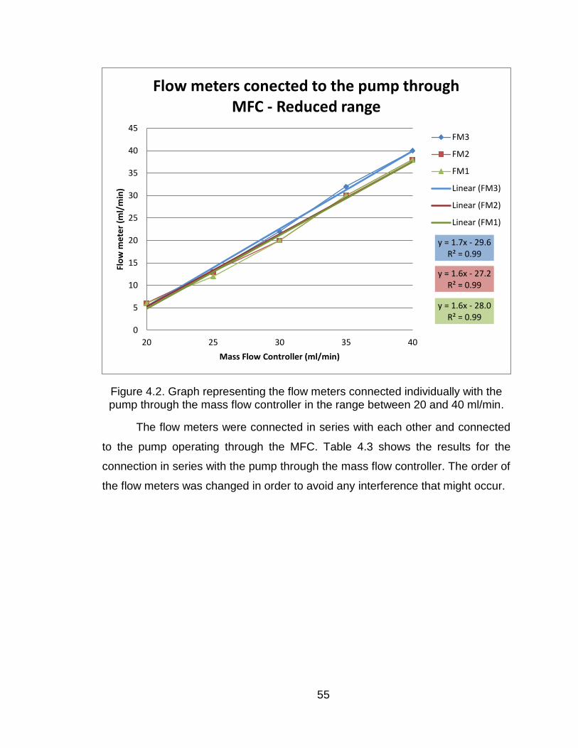
55

Figure 4.2. Graph representing the flow meters connected individually with the pump through the mass flow controller in the range between 20 and 40 ml/min.

The flow meters were connected in series with each other and connected

to the pump operating through the MFC. Table 4.3 shows the results for the

connection in series with the pump through the mass flow controller. The order of

the flow meters was changed in order to avoid any interference that might occur.

y = 1.7x - 29.6 R² = 0.99

y = 1.6x - 27.2 R² = 0.99

y = 1.6x - 28.0 R² = 0.99

0

5

10

15

20

25

30

35

40

45

20 25 30 35 40

Flo

w m

ete

r (m

l/m

in)


Flow meters conected to the pump through MFC - Reduced range

FM3

FM2

FM1

Linear (FM3)

Linear (FM2)

Linear (FM1)

56

Table 4.3. Results for flow meters connected in series with the pump through the

mass flow controller.

Order Flow meter MFC (20 mL.min-1) MFC (25 mL.min-1)

1-2-3

1 3 8

2 3 8

3 4 9

2-3-1

1 2.5 5.5

2 4.5 10

3 3.5 7.5

3-1-2

1 1.8 4.5

2 2 5.5

3 2.5 8

An important observation from Table 4.3 which first suggested the idea of

the unbalanced nature of these flow meters at lower flows was made when one

realized the mass flow controller was set to 20 and 25 mL.min-1. The flow meters

showed a maximum reading of 10 mL.min-1. Here the order of the flow meters did

not show significant difference with P-values of 0.48 and 0.32 for 20 and 25

mL.min-1 respectively (Appendix B).

Concern regarding the pulsing nature of the diaphragm pump as a flow

source resulted in a set of companion tests using a compressed air tank as the

source. The results presented in Table 4.4 correspond to the use of the tank

connected with the flow meters individually.

57

Table 4.4. Results of the flow meters individually connected to the tank and the

mass flow controller.

MCF (mL.min-1) FM3 (mL.min-1) FM2 (mL.min-1) FM1 (mL.min-1)

20 25 28 25

25 32.5 30 30

30 37.5 37.5 35

35 42.5 43 40

40 49 45 45

45 50 50 50

50 52.5 52.5 53

The data in this experiment (Figure 4.3) suggest that the range of good

agreement for the flow meters is larger, ranging from 20 to 50 ml/min. That can

be observed through the R2 of the linear regressions that are all above 0.95 and

with very similar coefficients for regressions through an ANNOVA with the P-

value of 0.95 (Appendix B). This may be attributable to having sufficient

pressure at the tank to overcome the pressure drop imposed by the MFC.

58

Figure 4.3. Graphic representing the flow meters connected to the tank individually through the mass flow controller.

The flow meters were then connected in series with the tank through the

mass flow controller. The results are presented in Table 4.5, where the flow

meters had their order changed similar to the test when connected to the pump in

order to avoid any error that might occur as a consequence of the order. The

results presented high P-values which indicate that there were no significant

differences when the order was changed (Appendix B).

y = 0.92x + 9.0 R² = 0.95

y = 0.86x + 10.6 R² = 0.97

y = 0.95x + 6.2 R² = 0.99

20

25

30

35

40

45

50

55

20 25 30 35 40 45 50

Flo

w m

ete

r (m

l/m

in)


Flow meters conected to the air cylinder through MFC

FM3

FM2

FM1

Linear (FM3)

Linear (FM2)

Linear (FM1)

59

Table 4.5. Results for the flow meters connected in series with the air tank

through the mass flow controller.

Flow meter MFC (20 mL.min-1) MFC (25 mL.min-1)

1-2-3

1 17.5 22.5

2 25 30

3 25 30

2-3-1

1 12.5 15

2 25 32.5

3 17.5 28

3-1-2

1 10 15

2 18 22.5

3 15 20

The tests with flow meters indicated that all three of them were working

properly and in agreement with each other eliminating the hypothesis of flow

imbalances from the flow meters.

4.1.2 Chamber leakage

Tests were conducted to find leakage within the biofilter chambers that

could have compromised their operation by creating different pressure conditions

within the chambers. Various points in the structure were evaluated for leakage,

with special attention given to the joints where the wood was glued together.

The analyses using smoke tests were made visually. Wherever there was

smoke coming out of the biofilter other than the exhaust, a leakage point was

identified. During the test the smoke was flowing uniformly across the media, with

a linear front rising from the bottom to the top of the media (Figure 4.4).

60

Figure 4.4. Smoke rising to the media surface.

This behavior of the smoke was an indication that no preferential

pathways were forming in the media while the tests were being performed.

Preferential pathways are a problem for the biofilters because the airflow can

pass faster which in turn, can reduce the percentage of the biofilter bacterial

population exposed to the ammonia in the air for metabolization.

No major leaks were found in the chambers. However, a very small leak

was noticed between the chamber and the cone at one corner on biofilter #3 and

also under biofilter #1 through a crack at the bottom of the plenum. After some

discussion it was decided that this leakage was not significant to the biofilter

performance and also did not have an effect on the performance of the other

biofilters.

A smoke test was performed in biofilter #1 with the outlet plugged

expecting that some pressure would build up within the biofilter. This was done

to simulate the pressure caused by the air coming from the blower and therefore

some smoke would escape from any possible leaking points. Unfortunately, the

smoke machine was not able to produce sufficient pressure and the smoke

61

merely exiting from the hose supplying the smoke. Hence, this test was not able

to conclude anything about possible leaks when the biofilter is pressurized.

Therefore it was not repeated for the other two biofilters.

4.1.3 Balancing the system: exhaust side

An important observation made during the smoke test happened when the

exhaust system was turned on. It could be seen in biofilter 1 that the exhaust

system was drawing the smoke thoroughly in a well-defined shape (Figure 4.5).

The exhaust stream was less well-defined over biofilter number 2, which

indicated the possibility of slight back pressure at the exhaust hood (Figure 4.6).

This pattern was even more noticeable over biofilter number 3 (Figure 4.7).

These differences may have been indictors of non-uniform conditions within the

test chambers which could mean a higher gas flow in a biofilter. After some

consideration it was concluded that was not the reason for the unexpected

values for biofilter number 3. It was reasoned that the potential back pressure

created by the exhaust fan above biofilter 3 was not responsible for the behavior

reported in Sales (2008) because the chaotic formation of the smoke during the

test was outside the biofilter. There was insufficient pressure in the biofilter from

the smoke machine to create positive pressure in the biofilter; still the smoke was

coming out the biofilter. This suggests that during the actual tests when the

biofilter is under pressure, this back pressure from the exhaust fan is small

enough to be considered negligible or does not exist and therefore would not

constitute a source of error.

62

Figure 4.5. No back pressure over biofilter 1.

Figure 4.6. Slight back pressure over biofilter 2.

63

Figure 4.7. Showing back pressure over biofilter 3.

4.1.4 Balancing the system: supply system side

The supply system was tested to check if the three biofilters were

operating under the same conditions during the tests. It was important to

determine whether the air flow supplied to them was the same. Two treatments

were performed while testing the supply system. One treatment operated the

system with the balancing damper over the plenum open and the other with the

damper closed.

The p-value of the averages of the air speed coming out of the plenum

was calculated for comparison. The results of that analysis show that there was a

significant difference between the biofilters when the damper was opened (Table

4.6). The Tukey analysis for means difference shows that biofilter 2 and 3 are not

significantly different, but that both are different from biofilter 1 (Table 4.7).

Table 4.6. Anova test for the air supply system with the damper open.

Source DF Type III SS Mean Square ((m.sec-1)2) F-Value Pr > F

Biofilter 2 0.503 0.25167 66.62 <0.0001

64

Table 4.7. Tukey grouping for the air supply system with the damper open.

Tukey Grouping Mean (m.sec-1) N Biofilter

A 6.5 6 3

A 6.5 6 2

B 6.2 6 1

Error mean square 0.0038

Table 4.8 shows the p-values for the treatment where the damper was

closed and sealed. The results show the p-value is high which means no

significant difference exists between biofilters. The equilibrium among the

biofilters is further proven with the Tukey analysis in Table 4.9, where the test

classifies all biofilters as being in the same group.

Table 4.8. Anova test for the air supply system with the exhaust duct closed.

Source DF Type III SS Mean Square ((m.sec-1)2) F-Value Pr > F

Biofilter 2 0.191875 0.0959375 0.02 0.9814

Table 4.9. Tukey grouping for the air supply system with the exhaust duct closed.

Tukey Grouping Mean (m.sec-1) N Biofilter

A 6.3 6 2

A 6.3 6 1

A 6.2 6 3


4.2 Sieve shaker machine

The new add-on component increased the performance of sieving

significantly. The compost was sieved at a rate of 0.272 m3.h-1 for the medium

gradation. This rate represented a total throughput of 2.092 cubic meters per

hour, which represents about 2.75 trips of a skid steer loader per hour.

65

4.3 Physical properties

4.3.1 Particle size distribution

As-received compost was sieved in order to measure the different portions

of particles sizes that are present in the media. After the measurement the total

of the particle sizes, used on this experiment comprised 48% (140 g) of the total

amount of compost measured. Material with a particle size bigger than 12.5 mm

represents 3% (9.325 g), large material 8% (22.975 g), medium material 13%

(37.55 g), small material 27% (79.35 g) and the finer material with diameter

smaller than 1.35 mm represents 49% (146.55 g) of the total (Figure 4.8).

Figure 4.8. As received compost particle size distribution.

Previous research has shown that the presence of fines in the as-received

compost, such as that used in the field, can contribute to the formation of

preferential air ways and also significant pressure drops which are problematic

for airflow (Sales, 2008). The material used for this experiment was comprised of

49% fines which further underscore the importance of sieving material for

improved biofilter efficiency. These results are comparable with Sales, 2008,

9.3

23.0

37.6

79.4

146.6

0.0

20.0

40.0

60.0

80.0

100.0

120.0

140.0

160.0

Rocks Large Medium Small Fines

Compost Particle Size Distribution (g)

66

where the fines material comprised 46.3%. The other particle sizes were also

similar to within a +/- 5% range. This suggests that the compost produced at the

farm for this experiment was physically very similar to that used by Sales (2008)

in the earlier work and therefore an additional basis for comparison was

established.

This project used the medium particle size (between 4.75 and 8 mm),

which represented 13% (539 g) of the total amount of as received material. The

tests outlined for the biofilters required a total of 612 liters of sieved, medium

particle size material. This required a total of 4707 liters of as received compost

to be sieved. A total of 7700 liters of as received compost was sieved in order to

provide additional enough material for the supporting experiments. Compost

material ranging between 1.35 to 4.75 mm and 8 to 12.5 mm comprised a total of

4095 liters and was saved.

4.3.2 Compost water content

4.3.2.1 Moisture measurement - Direct method

A preliminary drying test was performed to characterize the drying front

curves for the different regions of the biofilters. Table 4.10 shows the movement

of the drying front through the media, with the lower part of the biofilter drying

faster than the regions above it.

67

Table 4.10. Moisture content wet basis representing the movement of the drying

front in the media.

Time (hours) B1 B2 B3

Lower Middle Upper Lower Middle Upper Lower Middle Upper

0 0.45 0.51 0.51 0.48 0.45 0.46 0.51 0.50 0.49

12 0.26 0.50 0.46 0.35 0.46 0.47 0.40 0.53 0.49

24 0.19 0.48 0.48 0.18 0.50 0.47 0.20 0.50 0.45

36 0.13 0.42 0.48 0.18 0.44 0.45 0.15 0.46 0.48

48 0.07 0.43 0.40 0.10 0.42 0.42 0.09 0.42 0.43

60 0.10 0.33 0.34 0.11 0.27 0.36 0.10 0.36 0.40

72 0.09 0.29 0.38 0.07 0.17 0.40 0.10 0.21 0.33

84 0.10 0.12 0.28 0.08 0.17 0.36 0.08 0.19 0.34

96 0.04 0.15 0.27 0.09 0.10 0.19 0.10 0.10 0.33

108 0.14 0.08 0.08 0.24 0.09 0.09 0.11 0.08 0.09

These data are presented graphically in Figure 4.9 to better represent the

drying front movement. It can be seen that the middle part just starts to dry after

the lower part reaches equilibrium in the moisture content, after about 50 hours

and the upper region starts to dry after about 70 hours.

68

Figure 4.9. Characterization of the drying front movement in the biofilter.

The individual biofilters were compared to determine if all three of them

were subjected to the same pattern of drying front movement. Figure 4.10 shows

the drying front in the lower region for the three biofilters, and indicates a drying

period in the firsts 52 hours of experiment and after this time the moisture content

reaches equilibrium with the supply air at approximately 10% wet basis. Table

4.11 shows that the P-Value for the equilibrium period is high which indicates that

the slopes are not significant different from zero and the drying period have a

significantly different slope from zero.

0.00

0.10

0.20

0.30

0.40

0.50

0.60

0 20 40 60 80 100 120

Mo

istu

re c

on

ten

t w

.b.

Time (hours)

Drying front movement

Lower

Middle

Upper

69

Table 4.11. P-values for the hose positioned in the lower position.

Lower Region P-Value

Equilibrium Period 0.0115

Drying Period <0.0001

Figure 4.10. Drying pattern for lower region.

Results for drying in the middle position are presented in Figure 4.11

where the data shows a drying front that started after 52 hours, when the lower

region reaches an equilibrium at 10% w.b.. This is important information because

it is possible to assume that the lower region worked as a buffer for the regions

above it allowing them to dry after the lower region have reached equilibrium.

This equilibrium period and drying period are described by the Table 4.12 and

the statistical analyses are in the Appendix C, where it is possible to see that the

three biofilters are working similarly.

70

Table 4.12. P-values for the hose positioned in the middle position.

Middle Region P-Value



Figure 4.11. Drying pattern for middle region.

Figure 4.12 is the graphical representation of the drying front in the upper

position of the three biofilters. It is possible to see that there are two distinctive

periods of drying: the first period is the equilibrium period when the moisture

content is kept constant. This is the period where the biofilter media is in

moisture equilibrium with the air exiting the middle region. The second period is

the drying period that starts at 60 hours just few hours after the middle region

starts to dry and the lower reaches equilibrium, Table 4.13 shows the p-values

for these periods during the experiment and the statistical analysis are in the

Appendix C.

71

Table 4.13. P-values for the hose positioned in the upper position.

Upper Region P-Value



Figure 4.12. Drying pattern for upper region.

With all this information it can be concluded that the medium and upper

region dries out after the lower region reaches equilibrium moisture content. The

lower region is a moisture buffer zone for the biofilter which indicates the critical

need for moisture content control in this region. It could be assumed once the

moisture is maintained in equilibrium at the designed level in the lower region the

other regions would be protected.

Table 4.14 shows the P-values for the contrasts between the biofilters

where they are all high values which means that the three biofilters are working

similarly as replicates. Appendix C shows the statistical analysis for these

contrasts.

72

Table 4.14. P-values for the contrasts between the biofilters.

1 vs 2 1 vs 3 2 vs 3

Dry Period

Lower 0,89 0,41 0,34

Middle 0,54 0,75 0,35

Upper 0,47 0,94 0,51

Equilibrium

Lower 0,22 0,52 0,06

Middle 0,04 0,46 0,16

Upper 0,31 0,53 0,7

4.3.2.2 Moisture measurement - Indirect method

A curve for thermal conductance and moisture content was developed

using three replicates of eight media moisture content for the medium size range.

This measurement resulted in the graphical representation shown in Figure 4.13

and presented an R2 of 0.925 for an exponential regression.

Figure 4.13. Thermal conductance exponential regression for compost medium particle sizes.

A second regression analysis was performed on the range between 30

and 50% because this was the range of moisture content in which a biofilter

y = 0.0569e3.1789x R² = 0.925

0

0.1

0.2

0.3

0.4

0.5

0.6

0.7

0.8

10% 20% 30% 40% 50% 60% 70%

The

rmal

Co

nd

uct

ance

(W

/m.K

)

Moisture content w.b. (%)

Thermal Conductance for medium particle size

73

would normally operate. In this case the data presented a different pattern as

presented in Figure 4.14 where a linear regression with a R2 of 0.85 was fitted to

the data. The standard error for the operational range regression is presented in

Table 4.15 with a value of 0.02.

Figure 4.14. Thermal conductance linear regression for compost medium particle sizes.

y = 0.504x - 0.0204 R² = 0.8588

0

0.05

0.1

0.15

0.2

0.25

0.3

30% 35% 40% 45% 50% 55% 60%

The

rmal

co

nd

uct

ance

(W

/m.K

)


Thermal Conductance

74

Table 4.15. Regression analysis for thermal conductance on the operational

range of the biofilter.

The medium particle size presented an R2 equal to 0.859 relating moisture

content to thermal conductivity. The moisture content of the biofilters is intended

to fall within this narrower range because of it encompasses the limits of

microbial activity on the lower end and reasonable levels of ammonia conversion

without the danger of nitrous oxide production on the upper end. Based on the

exponential regression equation 4.1 was be used during the performance tests to

measure the water present in the compost and estimate the amount of water to

be applied to maintain the target media moisture content.

4.1

= Moisture content (wet basis)

= Thermal conductance read in the sensor (W/m.k)

The use of this sensor presented the possibility of error in the

measurement from partial insertion of the probe into the compost. The initial

calibration experiments were performed with the probe entirely inserted into the

compost mass. However, when the system was used in the biofilter there would

be a difference in the inserted depth owing to the thickness of the biofilter

plywood wall.

75

A test was conducted to measure the effect of the depth of the probe in

the compost mass. Five treatments were chosen, entirely inside the mass, 2/3

and 1/3 of the needle inserted into the media and also with plywood covering a

portion of the probe. The plywood itself had two treatments: wet and dry, in order

to consider the water absorption of the biofilter wall. Three replicates and three

moisture contents were used for this experiment with the results presented in

Table 4.16.

Table 4.16 Thermal conductance (W/m.K) for different depths of the metal probe

in the compost mass.

35% 45% 55%

1

0.210 0.212 0.315

0.234 0.179 0.249

0.203 0.214 0.556

2/3

0.173 0.172 0.176

0.161 0.180 0.144

0.176 0.173 0.175

1/3

0.144 0.096 0.104

0.107 0.108 0.125

0.111 0.099 0.091

Plywood dry

0.160 0.205 0.159

0.227 0.180 0.209

0.188 0.186 0.243

Plywood wet

0.195 0.181 0.190

0.181 0.227 0.207

0.156 0.187 0.225

76

A statistical comparison between the depths was performed in order to

determine any difference among the results of thermal conductance and the

condition of the treatment. The results of that analysis are presented in Table

4.17.

Table 4.17. Statistical output for the different probe depths test.

Moisture (% w.b.)

Depth Depth Estimate (W/m.K)

StdErr tValue P-

value

35

1

1/3 0.09 0.02 4.05 0.0003

2/3 0.04 0.02 1.71 0.0974

Plywood 0.02 0.02 0.91 0.3704

Plywood wet

0.03 0.02 1.43 0.1624

1/3

2/3 -0.05 0.02 -2.34 0.0261

Plywood -0.07 0.02 -3.14 0.0038

Plywood wet

-0.06 0.02 -2.62 0.0137

2/3

Plywood -0.02 0.02 -0.8 0.4291

Plywood wet

-0.01 0.02 -0.28 0.7823

Plywood Plywood

wet 0.01 0.02 0.52 0.605

45

1

1/3 0.11 0.02 4.63 <.0001

2/3 0.02 0.02 1 0.3244

Plywood 0.01 0.02 0.41 0.6846

Plywood wet

0.00 0.02 0.13 0.8962

1/3 2/3 -0.08 0.02 -3.63 0.001

Plywood -0.10 0.02 -4.22 0.0002

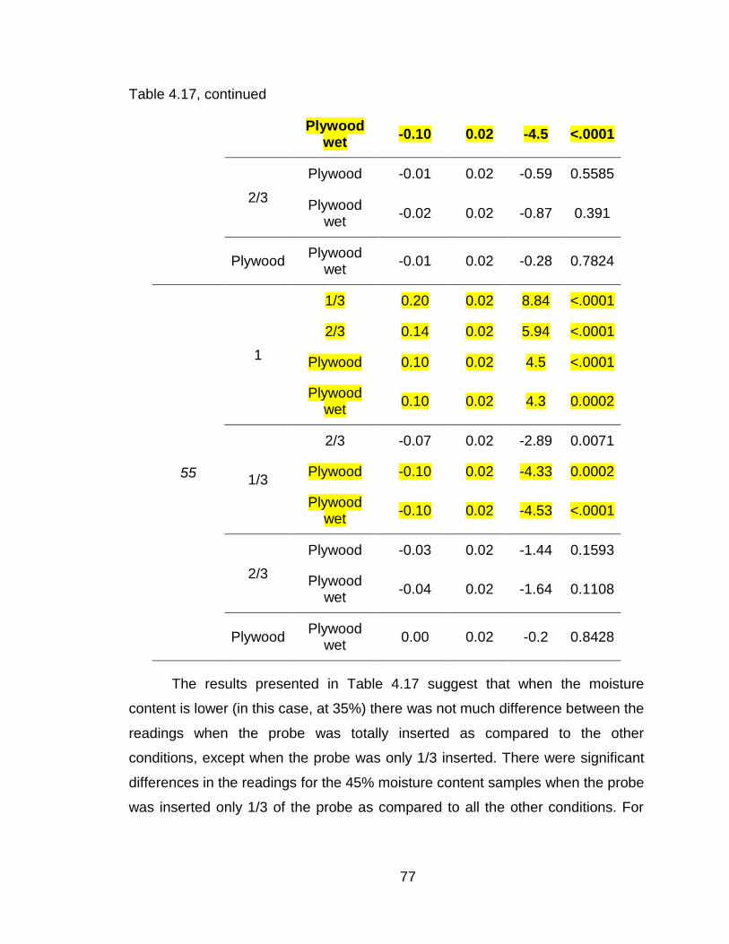
77

Table 4.17, continued

Plywood wet

-0.10 0.02 -4.5 <.0001

2/3

Plywood -0.01 0.02 -0.59 0.5585

Plywood wet

-0.02 0.02 -0.87 0.391

Plywood Plywood

wet -0.01 0.02 -0.28 0.7824

55

1

1/3 0.20 0.02 8.84 <.0001

2/3 0.14 0.02 5.94 <.0001

Plywood 0.10 0.02 4.5 <.0001

Plywood wet

0.10 0.02 4.3 0.0002

1/3

2/3 -0.07 0.02 -2.89 0.0071

Plywood -0.10 0.02 -4.33 0.0002

Plywood wet

-0.10 0.02 -4.53 <.0001

2/3

Plywood -0.03 0.02 -1.44 0.1593

Plywood wet

-0.04 0.02 -1.64 0.1108

Plywood Plywood

wet 0.00 0.02 -0.2 0.8428

The results presented in Table 4.17 suggest that when the moisture

content is lower (in this case, at 35%) there was not much difference between the

readings when the probe was totally inserted as compared to the other

conditions, except when the probe was only 1/3 inserted. There were significant

differences in the readings for the 45% moisture content samples when the probe

was inserted only 1/3 of the probe as compared to all the other conditions. For

78

55% samples there is significant difference of the readings for any condition

other than entirely inserted.

These results suggest that for any moisture condition it is important that

the probe stays more than 1/3 inserted into the compost to get a better

measurement. Further, with increased moisture content it was more important to

get the probe fully inserted into the compost. These analyses also indicated

embedment of the probe into the compost for a more accurate and reliable

measurement, instead of inserting it in the media through the biofilter wall.


4.4.1 Preliminary test and calibration

The preliminary test for drying the compost was the no hose treatment

used when analyzing the effects of vertical positions of the hoses. It was

performed in order to determine the amount of water that should be applied in the

biofilter to maintain given moisture content during operation. These results also

reinforce the movement of the drying front through the media pattern, with the

lower part of the biofilter drying faster than the upper part as shown in section

4.3.2.1 when the drying front’s curves were characterized.

79

Figure 4.15. Preliminary test for water demand calculation.

An average of 111 kg of wet compost was loaded into the three biofilters

with an initial moisture content of 47%, which translated to 58.6 kg of dry matter

and 52.5 kg of water.

0%

10%

20%

30%

40%

50%

60%

0 50 100 150 200

Mo

istu

re c

on

ten

t w

.b. (

%)

TIme (hours)

Preliminary drying test - Hose Positioning - No hose

Lower

Middle

Upper

80

Table 4.18 was used as the reference for calculating the most severe

drying rate during the test which occurred between 72 and 101 hours at the

upper region. However, based on the preliminary tests when the middle and

upper regions did not start to dry before the lower region reached equilibrium, it

was determined that the most severe drying rate occurred in the lower region

where the water loss reached 6.28 kg between 48 and 57 hours. This constituted

a water loss rate of 0.42 kg/h as show in Table 4.19. Details for water application

and calculation are shown in the Appendix E.

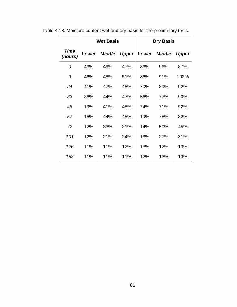
81

Table 4.18. Moisture content wet and dry basis for the preliminary tests.

Wet Basis Dry Basis

Time (hours)

Lower Middle Upper Lower Middle Upper

0 46% 49% 47% 86% 96% 87%

9 46% 48% 51% 86% 91% 102%

24 41% 47% 48% 70% 89% 92%

33 36% 44% 47% 56% 77% 90%

48 19% 41% 48% 24% 71% 92%

57 16% 44% 45% 19% 78% 82%

72 12% 33% 31% 14% 50% 45%

101 12% 21% 24% 13% 27% 31%

126 11% 11% 12% 13% 12% 13%

153 11% 11% 11% 12% 13% 13%

82

Table 4.19. Water Loss rate for the three regions of the biofilter.

Water Loss Rate (kg/h)

Time Lower Middle Upper

0 0.00 0.00 0.00

9 0.01 0.10 -0.33

24 0.21 0.03 0.14

33 0.30 0.25 0.04

48 0.42 0.09 -0.02

57 0.10 -0.15 0.21

72 0.07 0.37 0.48

101 0.01 0.15 0.09

126 0.01 0.12 0.14

153 0.00 -0.01 0.00

The highest drying rate for this process was used to calculate the

necessary water to be applied into the biofilter media. It was assumed that if the

system could supply enough water for this rate, then all the drying rates would

exceeded and the media would maintain its moisture content.

4.4.2 Soaker hose test

The soaker hoses were calibrated to determine the flow as a function of

pressure before being used in the biofilters. There were two steps involved in the

calibration. First, three meters of soaker hose were calibrated in order to find the

rate of flow per meter of hose. This information helped to determine the

appropriate length of hose to be placed in the media in order to supply enough

water to the biofilter. The hose was subjected to a series of pressures where the

amount of water collected and recorded are presented in Table 4.20. This

analysis was repeated three times. The results of the analysis along with a

prediction curve are presented in Figure 4.16.

83

Table 4.20. Calibration of soaker hoses

Pressure (kPa)

Flow (ml/s)

27.6 30.1

41.4 33.1

55.2 37.1

68.9 40.7

82.7 43.3

96.5 43.3

110.3 48.8

124.1 51.1

Figure 4.16. Linear regression of the soaker hose flow with the pressure.

The prediction model showed excellent agreement with the data resulting

in an R2 of 0.95. The model was used with the water requirements calculated in

y = 0.0518x + 7.783 R² = 0.9531

8

9

10

11

12

13

14

15

20 40 60 80 100 120 140

Wat

er

Flo

w p

er

me

ter

of

ho

se (

mL.

(s.m

)-1)

Pressure (Kpa)

Flow (mL.(s.mhose)-1)

Flow (mL.(s.m)-1)

Linear (Flow (mL.(s.m)-1))

84

the drying tests to define a length for the soaker hose to be installed in the

biofilter. The drying tests data indicated that the highest rate of water removal

from the biofilters was 420 grams of water per hour.

The equation for the hoses was created with three meters of hose, so the

equation can be transformed into a linear equation showing the flow results as a

function of the length. The equation then is transformed into the following.

4.2

= water flow (mL.(s.m)-1)

= pressure (kPa)

The flow is given in mL.(s.m)-1 of soaker hose and the pressure in kPa. It

was stipulated that the hose would work at a 68.95 kPa (10 psi) controlled by ball

valve and monitored by a pressure gauge. This is half of the maximum pressure

allowed in the soaker hose. The flow resulting from this pressure was 14.5 ml/s

over 1.2 m of soaker hose which required 5 minutes to apply all the water

necessary for the 12 hour period between readings.

4.4.3 Hose positioning (water added)

The hose positioning tests evaluated the performance of the soaker hoses

placed at three different positions in the biofilter which constituted the treatments

of this experiment. Compost samples were taken twice a day to monitor the

moisture content of the biofilters and water was applied to the biofilter right after

the sample was taken in order to avoid interference with the measurements.

Figure 4.17 shows the profile of moisture content in the biofilter when the

hose was positioned at the lower region. Figure 4.18 and Figure 4.19 shows the

SAS output for the moisture slopes in the lower and middle region and the p-

value calculated demonstrated that these slopes are not different from zero

which means constant moisture content. The upper region dried throughout the

extent of the experiment at a very low rate, but still the slope is not zero (Figure

4.20).

85

Figure 4.17. Chart showing the moisture content of the regions of biofilters with the hose installed in the lower position.

Figure 4.18. SAS output to the lower region when the hose is positioned in the lower region.

0

0.1

0.2

0.3

0.4

0.5

0.6

0.7

0 20 40 60 80 100 120

Mo

istu

re C

on

ten

t w

.b.

Time (hours)

Hose in Lower position

Lower

Middle

Upper

86


lower region.


lower region.

87

The hose when placed in the middle region allowed media drying (Figure

4.21), because its slopes were significantly different from zero as shown in

Figure 4.22, Figure 4.23 and Figure 4.24 in the SAS output with high p-value for

the slopes.

.

Figure 4.21. Chart showing the moisture content of the regions of biofilters with the hose installed in the middle position.

Figure 4.22. SAS output to the lower region when the hose is positioned in the middle region.

0%

10%

20%

30%

40%

50%

60%

70%

0 50 100 150 200

Mo

istu

re c

on

ten

t (%

)

Time (hours)

Hose in the Middle Position

Lower

Middle

Upper

88

Figure 4.23. SAS output to the middle region when the hose is positioned in the middle region.

Figure 4.24. SAS output to the upper region when the hose is positioned in the middle region.

The hose in the upper position (Figure 4.25) was able to bring the lower

region into an equilibrium moisture content of 30% w.b. after 20 hours as can be

seen in Figure 4.26 where the p value for the slope in the lower region after 20

hours is not significantly different from zero. The upper and middle regions were

drying (Figure 4.27 and Figure 4.28). One possible explanation for this could be

that the water was only passing through the media and not being absorbed by

the compost.

89

Figure 4.25. Chart showing the moisture content of the regions of biofilters with the hose installed in the middle position.

Figure 4.26. SAS output of the equilibrium period of the lower region when the hose is positioned in the upper region.

0%

10%

20%

30%

40%

50%

60%

70%

80%

0 20 40 60 80 100 120

Mo

istu

re c

on

ten

t (%

)

Time (hours)

Hose in the Upper Position

Lower

Middle

Upper

90

Figure 4.27. SAS output of the middle region when the hose is positioned in the upper region.

Figure 4.28. SAS output of the upper region when the hose is positioned in the upper region.

The installation of the soaker hose was a viable concept for delivering

water to the compost media, especially in the lower region where the hose was

able to keep the moisture at a level that sustains microbial activity throughout the

media over the extent of this experiment. Some drying was observed during the

process when the hose was placed in the middle and upper position. This could

be an indication of insufficient hose in the media, or that the shape of the hose

was not able to deliver the water accurately in the media or even that the water

was not being absorbed by the media.

The slopes of each region were contrasted among four treatments: no

hose, hose in lower, hose in middle and hose in upper. These contrasts were

constructed to find the treatment that was most different from the “no hose”

treatment when no water was applied.

91

Table 4.21. Contrasts of the moisture content slopes.

Contrasts

Label Num DF Den DF F Value Pr > F

No hose vs Lower 1 332 15.07 0.0001

Lower vs Middle 1 332 3.49 0.0625

No hose vs Middle 1 332 8.96 0.0030

No hose vs Upper 1 332 0.00 0.9727

Lower vs Upper 1 332 14.79 0.0001

Middle vs Upper 1 332 8.67 0.0035

The ANOVA results for this analysis are presented in Table 4.21. It is

possible to see that the moisture content slope in “lower” treatment is significantly

different from the “no hose” treatment. This is reasonable because the lower

position of the hose was able to maintain the moisture content. The hose in the

“middle” treatment was also significantly different from zero, but the reason is

that the drying rate was much lower than when “no hose” was applied. The

“upper” treatment did not show any difference from the “no hose” treatment

because of the drying of the upper and middle regions.

4.4.4 Water application interval

Water was applied for two minutes to the biofilter at different time intervals

in order to evaluate if there was any difference in the applied water draining from

the biofilter over different application times (Table 4.22).

92

Table 4.22. Water interval evaluation.

Time Biofilter Water (kg)

30 sec

1 0.85

2 1.1

3 1.35

120 sec

1 1.5

2 1.55

3 1.5

15 sec

1 1.55

2 1.5

3 1.55

A Tukey analysis was performed to test the differences between the

treatments (Table 4.23). The treatment with water being applied for 30 seconds

with two minutes interval is significantly different from others treatments with the

lower mean for water drainage.

Table 4.23. Tukey grouping for water interval tests.

Tukey Grouping Mean (kg of H2O) N Time (sec)

A 1.5333 3 15

A 1.5167 3 120

B 1.1000 3 30


Water applied for a total of two minutes during four applications of 30

seconds at two minute intervals presented the lowest mean for applied water

draining from the filter.

93

4.5 Ammonia and Nitrous Oxide Observations

4.5.1 Water balance

4.5.1.1 Direct Method

The Direct Method consisted of taking compost samples from the three

regions of the biofilter with a grabbing tool in a way that was representative of

that region. First, samples were taken once a day, but after the first week the

samples were taken every two days. The time interval was increased because

taking samples diminished the amount of compost and the process of taking

samples every day during the whole time of the experiment would be damaging

for the compost mass.

The moisture content for each of the three regions of the biofilters is

represented in Figure 4.29 and Figure 4.30. When no water was applied to the

compost, it was possible to see a fast drying rate for the lower region which

reaches 10% w.b. moisture content after approximately 100 hours. The middle

region began to dry right after this region gets to 20% w.b. The upper region of

the biofilter was the region with the slowest drying rate reaching 20% moisture

content after 350 hours.

The treatments where water was applied to the compost were

characterized by higher levels of moisture content which maintained microbial

activity for the whole extent of the experiment. The lower region started to dry,

but it was maintained above levels required that support microbial activity.

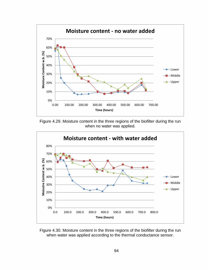
94

Figure 4.29. Moisture content in the three regions of the biofilter during the run when no water was applied.

Figure 4.30. Moisture content in the three regions of the biofilter during the run when water was applied according to the thermal conductance sensor.

0%

10%

20%

30%

40%

50%

60%

70%

0.00 100.00 200.00 300.00 400.00 500.00 600.00 700.00

Mo

istu

re C

on

ten

t w

.b. (

%)

Time (hours)

Moisture content - no water added

Lower

Middle

Upper

0%

10%

20%

30%

40%

50%

60%

70%

80%

0.0 100.0 200.0 300.0 400.0 500.0 600.0 700.0 800.0

Mo

isu

tre

Co

nte

nt

w.b

. (%

)

Time (hours)

Moisture content - with water added

Lower

Middle

Upper

95

Water was applied to the compost based on moisture content readings

taken four times a day with the thermal capacitance meter. Figure 4.31 shows

the drying front in the lower region for the two treatments. The data for the two

treatments presented the same pattern but in the treatment with water the lower

region may have worked as buffer for the regions above, as can be seen in

Figure 4.32. This likely occurred when the soaker hoses kept the minimum

moisture content of the middle region above 50% w.b. The upper region

presented the same pattern of drying as the lower region but at higher moisture

content (Figure 4.33).

These shifts in the drying curves are important because it elevates the

overall moisture content of the biofilters. This is important because biological

activity ceases at moisture content lower than 17% w.b.(water activity < 0.95) for

this media (Del Nero Maia, 2010).

Figure 4.31. Lower region drying fronts comparison between the treatments with no water and water applied.

0%

10%

20%

30%

40%

50%

60%

70%

80%

0.00 100.00 200.00 300.00 400.00 500.00 600.00 700.00 800.00

Mo

istu

re c

on

ten

t w

.b. (

%)

Time (hours)

Lower region moisture content

No water

Water

96

Figure 4.32. Middle region drying fronts comparison between the treatments with no water and water applied.

Figure 4.33. Upper region drying fronts comparison between the treatments with no water and water applied.

0%

10%

20%

30%

40%

50%

60%

70%

80%

0.00 100.00 200.00 300.00 400.00 500.00 600.00 700.00 800.00

Mo

istu

re c

on

ten

t w

.b. (

%)

Time (hours)

Middle region moisture content

No water

Water

0%

10%

20%

30%

40%

50%

60%

70%

80%

0.00 100.00 200.00 300.00 400.00 500.00 600.00 700.00 800.00

Mo

istu

re c

on

ten

t w

.b. (

%)

Time (hours)

Upper region moisture content

No water

Water

97

Without the water application the biofilters reached a moisture content

threshold that does not support biological activity after 100 hours in the lower

region, 300 hours in the middle and 450 hours in the upper region. Conversely,

with the water being applied the biofilters did not reach this limit for the extent of

the experiment.

Calculation of the water loss rate in this experiment allowed a better

understanding of the water behavior in the biofilters when comparing

measurement methods, because the water content values were all in Kg.

Table 4.24 shows the biofilter loses a total of 77.2 kg of water during the

entire time of the experiment (647 hours of operation).This is a considerable

amount of water taking into consideration that the initial amount of water in the

biofilter was 88 kg. Drying removed about 87% of the initial water, taking into

consideration that this treatment represented no water replacement.

98

Table 4.24. Mass of water lost in the biofilter when no water is applied into the

media.

No Water

Time (hours)

Lower (kg)

Middle (kg)

Upper (kg)

0 22.4 25 26.2

17 29.5 28.7 23.8

40 6 26.6 18

64 4.4 26.3 15.1

136 1.6 10.6 8.7

160 1.3 7.3 7

189 1.3 5.8 6.3

238 1.4 4.8 6.7

303 1.8 2 5.1

351 1.5 1.4 4.6

400 1.5 1.6 3.4

448 1.8 2.2 2.5

496 1.8 2.1 3.9

520 1.5 1.6 2.9

616 3.7 4.4 5.8

647 2.2 2.3 2.7

Total Loss (kg)

27.3 26.4 23.5

99

Table 4.25 shows the final water loss which corresponded to the

difference between the initial and the final water content of the experiment for the

treatment when water was being applied to the compost to compensate for the

drying. It is possible to see that drying occurred but at a lower rate than the no

water treatment. Table 4.26 presents the total water lost which is the amount of

water lost throughout the experiment and accounting for the water that was

applied by the hoses. This represents the actual amount of water removed from

the compost.

100

Table 4.25. Water loss for the biofilter when water is applied into the media.

Water

Time (h)

Lower (kg)

Middle (kg)

Upper (kg)

0 30.2 31.8 31

20 21.2 20.3 29.9

43 23.4 25.8 33.9

67 22.6 32.4 30.4

91 16.6 25.6 30

115 10.6 28.6 26.2

139 7.6 23.5 19.9

233 4.5 21.4 16.2

281 4.1 22.5 19

338 4.4 14 12.3

382 3.8 12.8 14.7

425 5.7 21.8 12.2

472 5.8 14.9 11.6

547 13.2 18 11.1

619 7.5 15.3 9.3

712 6.5 15.3 7.7

713 6.5 15.5 9.4

Total Loss (kg)

23.7 16.9 24.5

101

Table 4.26. Water loss for the biofilter treatment for water applied into the media,

taking into consideration the water added during the process.

Water

Time (h) Lower

(kg) Middle

(kg) Upper (kg)

0 9.1 11.5 1.1

20 0 0 0

43 0.8 0 3.5

67 6 6.9 0.4

91 6 0 3.7

115 2.9 5.1 6.3

139 3.1 2.1 3.8

233 0.4 0 0

281 0 8.5 6.7

338 0.6 1.2 0

382 0 0 2.5

425 0 6.9 0.7

472 0 0 0.5

546 5.7 2.6 1.8

619 1 0 1.5

712 0 0 0

713 0 0 0

Total Loss (kg)

35.7 44.8 32.5

102

Table 4.21 shows that drying represented 70% of the total initial water

amount in the biofilter. Based on this data, it is inferred that there was a 17%

reduction in the moisture loss by the media.

4.5.1.2 Photoacoustic gas analyzer

The INNOVA 1412 is a photoacoustic gas analyzer that measures the

amount of water vapor as well as other gases present in a sample. It was used

during the experiment to track the water vapor in the gas stream across all the

regions of the biofilter by determining the increase in water content of the gas

phase.

Sampling ports were installed in five regions in the biofilter: plenum, lower,

middle, upper and headspace. This was necessary to create a profile of the

water loss across the media. The INNOVA gives the amount of water in the air as

mgh2o/m3air. Figure 4.34 is a graphic representation of the amount of water in

the gas phase in the five regions of the biofilters during the treatment of water

being applied.

Figure 4.34. Water vapor profile in the biofilter.

103

The water loss in the biofilter as measured by the INNOVA was calculated

in kg of water to generate a comparison to the oven tests. The airflow was used

to calculate the amount of water that was removed from the compost. To

calculate the water removed from the biofilter, the difference between the

headspace water vapor content and the laboratory air water vapor contents was

calculated.

The laboratory air had an average of 25oC and 57% relative humidity

which gave an average of 9,500 mg/m3 of water vapor. The average air flow was

95 m3/h. The water removed from the biofilter was determined by calculating the

difference of water content of the air coming out of the headspace from the water

content of the laboratory air with equation 4.3.

4.3

= Water removal (mg/m3)

= Headspace air water content (mg/m3)

= Laboratory air water content (mg/m3)

This water removal (Figure 4.35) was then multiplied by the air flow to find

the mass of water being removed from the compost which gave the rate of water

loss in g/h of water removed.

The water loss rate can be multiplied the time interval between readings to

find the water mass removed. The total amount of water lost based on the Innova

measurements is 308 kg of water during 691 hours of experiment.

104

Figure 4.35. Water removed from the biofilter.

4.5.1.3 Thermal conductance

The values for thermal conductance vs. time in the compost biofilter are

presented in Figure 4.36. Three measuring points were used on the wall of the

biofilter to measure the thermal conductance of the compost during the

abatement test.

0

1000

2000

3000

4000

5000

6000

7000

8000

9000

0 100 200 300 400 500 600 700 800

Wat

er

rem

ova

l (m

g/m

3)

Time (hours)

Water removal

105

Figure 4.36. Thermal conductance in the biofilter compost in the three regions.

The values for thermal conductivity were transformed into equivalent

moisture contents using the calibration equation 4.1. The results are presented

in Figure 4.38. The data indicate that this material reached equilibrium after 250

hours for all three regions. As indicated by the SAS output in the Figure 4.37

because of the high p-value which means no significant difference with a zero

slope.

Figure 4.37. SAS output for the thermal conductance readings after 250 hours.

0.05

0.10

0.15

0.20

0.25

0.30

0 100 200 300 400 500 600 700

The

rmal

Co

nd

uct

ance

(w

/m.K

)

Time (hours)

Thermal Conductance

Lower

Middle

upper

106

Figure 4.38. Calculated moisture content based on the equation 4.1 calibrated for thermal conductance.

The discrepancy between moisture content as compared to the direct

moisture content was first attributed to the fact that the thermal conductivity

probe was not entirely inserted into the compost. However, as reported in

Section 4.2.2.3, this hypothesis was discarded.

Thermal conductance did not show good performance for a reason not yet

defined.

0%

10%

20%

30%

40%

50%

60%

0 100 200 300 400 500 600 700 800

Mo

istu

re c

on

ten

t w

.b. (

%)

TIme (hours)

Thermal conductance moisture content

Lower

Middle

upper

107

Figure 4.39. Comparison of the moisture content calculated by the thermal conductance method with the oven method at the lower position of the biofilters.

The lower position showed that for both methods of measurements the

regression has high R2, and that the thermal conductance method presented an

offset of the actual data.

Comparisons on the middle and upper regions are presented in Figure

4.40 and Figure 4.41 respectively. In these two regions the thermal conductance

measurements also indicated an offset of the actual moisture content.

y = -3E-09x3 + 4E-06x2 - 0.0018x + 0.3712 R² = 0.8287

y = -7E-09x3 + 9E-06x2 - 0.0038x + 0.7419 R² = 0.8797

0%

10%

20%

30%

40%

50%

60%

70%

80%

0 100 200 300 400 500 600 700 800

Mo

istu

re c

on

ten

t w

.b. (

%)

Time (hours)

Lower

Thermal ConductanceOvenPoly. (Thermal Conductance)Poly. (Oven)

108





y = -1E-09x3 + 2E-06x2 - 0.001x + 0.3642 R² = 0.7085

y = 7E-10x3 - 4E-07x2 - 0.0002x + 0.669 R² = 0.6584

0%

10%

20%

30%

40%

50%

60%

70%

80%

0 100 200 300 400 500 600 700 800

MO

istu

re C

on

ten

t w

.b. (

%)

Time (hours)

Middle


y = -1E-09x3 + 2E-06x2 - 0.0008x + 0.2932 R² = 0.5131

y = 3E-10x3 + 4E-08x2 - 0.0006x + 0.7094 R² = 0.9552

0%

10%

20%

30%

40%

50%

60%

70%

80%

0 100 200 300 400 500 600 700 800

Mo

istu

re c

on

ten

t w

.b. (

%)

Time (hours)

Upper


109

4.5.2 Ammonia Removal

Ammonia concentrations were measured using a photoacoustic gas

analyzer at five points in the biofilter in order to develop a profile of the ammonia

conversion. The removal efficiency of each region is graphically represented in

Figure 4.42, Figure 4.43, Figure 4.44 and Figure 4.45, where a negative number

means ammonia production and a positive number means ammonia reduction.

4.5.2.1 No moisture control

The lower biofilter region had high removal efficiency that rose to 90% in

biofilter 1 and approximately 60% in biofilters 2 and 3 as can be seen in Figure

4.42 while biofilters 2 and 3 leveled out at around 60%. The removal efficiency

remained relatively constant for the three biofilters after 50 hours of the

experiment.

Figure 4.42. Ammonia removal efficiency for the lower region with no water.

The ammonia removal efficiency in the middle biofilter position when no

water was applied is found in Figure 4.43. The removal efficiency remained in the

zero to 20% range for biofilters 2 and 3. Biofilter 1 indicated that ammonia was

-0.6

-0.4

-0.2

0.0

0.2

0.4

0.6

0.8

1.0

1.2

0 100 200 300 400 500 600 700

Re

mo

val E

ffic

ien

cy

Time- hr

Lower - No water

Biofilter 1 R1 Biofilter 2 R1 Biofilter 3 R1

110

generated. With the moisture content of the media at 10% (Figure 4.32), there

was no microbial activity to support ammonia generation. The position of the gas

sampling tube for this region may have been located in an area where there was

short circuiting the gas through a media section where there was low conversion

or adsorption due to no uniformity of media moisture as seen in Figure 4.38 and

Figure 4.55.

Figure 4.43. Ammonia removal efficiency for the middle region with no water.

The upper biofilter region (Figure 4.44) indicated that biofilter 2 was

generating some ammonia. Again, Figure 4.33 indicates that the media moisture

content was less than 20% which does not support microbial activity and

indicates short circuiting as discussed in the previous paragraph. Biofilter 1 had

low removal efficiency and biofilter 3 had removal efficiency around 20%.

-0.6

-0.4

-0.2

0.0

0.2

0.4

0.6

0.8

1.0

1.2

0 100 200 300 400 500 600 700

Re

mo

val E

ffic

ien

cy

Time- hr

Middle - No water


111

Figure 4.44. Ammonia removal efficiency for the upper region with no water.

There was some removal in the layer of media between the upper region

sampling port and the headspace sampling port but at a very low rate (Figure

4.45). When the biofilter was analyzed as a whole the overall ammonia removal

efficiency was calculated by the difference between the inlet and outlet

concentrations (Figure 4.46) and in this case biofilter 3 had the higher ammonia

removal rate.

-0.6

-0.4

-0.2

0.0

0.2

0.4

0.6

0.8

1.0

1.2

0 100 200 300 400 500 600 700

Re

mo

val E

ffic

ien

cy

Time- hr

Upper - No water


112

Figure 4.45. Ammonia removal efficiency for the headspace region with no water.

Figure 4.46. Ammonia removal efficiency for the overall biofilter with no water.

-0.6

-0.4

-0.2

0.0

0.2

0.4

0.6

0.8

1.0

1.2

0 100 200 300 400 500 600 700

Re

mo

val E

ffic

ien

cy

Time- hr

Headspace - No water


0.0

0.1

0.2

0.3

0.4

0.5

0.6

0.7

0.8

0.9

1.0

0 100 200 300 400 500 600 700

Re

mo

val E

ffic

ien

cy

Time- hr

Overall - No water

Biofilter 1 Biofilter 2 Biofilter 3

113

Low moisture content biofilters (no microbial activity) that still have

ammonia removal, especially in the lower region (Figure 4.47) exhibit ammonia

adsorption to the solid media by hydrogen bonding (Liberty, 2001). Liberty (2001)

reported that compost can hold up to 1.6 gmol of ammonia per kilo of dry matter

of compost for media moisture content near zero. Therefore, the biofilters filled

with 51 kg of dry mass would potentially hold up to 81.6 gmol of ammonia. A

nitrogen balance on the biofilters with no moisture control can account for the

removal efficiency of ammonia when moisture no longer supported microbial

activity. This can explain the ammonia removal efficiencies in the lower region.

Figure 4.47. Graphical representation of the moisture content and the ammonia removal of the lower region during the treatment when no water is being added.

Ammonia removal efficiency in the middle region had two distinctive

phases (Figure 4.48). The first phase had sufficient moisture content in the

compost until around 250 hours to sustain biological activity and therefore

ammonia removal. After 250 hours, the moisture decreased to below 10% w.b.

and biological activity ceased. There was some ammonia generation after 250

-0.4

-0.2

0

0.2

0.4

0.6

0.8

0 100 200 300 400 500 600 700

Mo

istu

re C

on

ten

t an

d A

mm

on

ia R

em

ova

l (%

)

Time (hours)

Lower region: moisture content x ammonia removal

Moisture content Ammonia removal

Stable range

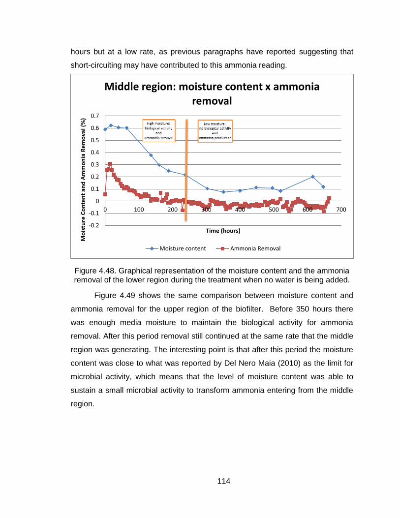
114

hours but at a low rate, as previous paragraphs have reported suggesting that

short-circuiting may have contributed to this ammonia reading.


Figure 4.49 shows the same comparison between moisture content and

ammonia removal for the upper region of the biofilter. Before 350 hours there

was enough media moisture to maintain the biological activity for ammonia

removal. After this period removal still continued at the same rate that the middle

region was generating. The interesting point is that after this period the moisture

content was close to what was reported by Del Nero Maia (2010) as the limit for

microbial activity, which means that the level of moisture content was able to

sustain a small microbial activity to transform ammonia entering from the middle

region.

-0.2

-0.1

0

0.1

0.2

0.3

0.4

0.5

0.6

0.7

0 100 200 300 400 500 600 700

Mo

istu

re C

on

ten

t an

d A

mm

on

ia R

em

ova

l (%

)

Time (hours)

Middle region: moisture content x ammonia removal

Moisture content Ammonia Removal

115


The removal of ammonia during the no water added test could have

resulted from three factors: bacterial activity until 400 hours would have had

sufficient moisture to support biological activity, absorption of ammonia by the

compost mass and the rest was accounted for in the inefficiency of the system,

because the biofilters were not 100% efficient for ammonia removal.

4.5.2.2 Moisture control

Figure 4.50 showed that the lower regions of biofilters 2 and 3 generated

ammonia until about 150 hours while biofilter 1 presented the higher ammonia

removal efficiency. The initial production was from the re-equilibrium of the initial

inoculums species die-off that generated ammonia.

-0.1

0

0.1

0.2

0.3

0.4

0.5

0.6

0.7

0.8

0 100 200 300 400 500 600 700

Mo

istu

re C

on

ten

t an

d A

mm

on

ia R

em

ova

l (%

)

Time (hours)

Upper region: moisture content x ammonia removal


116

Figure 4.50. Ammonia removal efficiency for the lower region with water.

The middle biofilter region had the most unusual behavior for ammonia

removal (Figure 4.51). In this region biofilter 1 had a peak of ammonia generation

and settled at a 30% generation level while biofilter 2 had a peak of removal and

settled at 80% removal.

-1.0

-0.8

-0.6

-0.4

-0.2

0.0

0.2

0.4

0.6

0.8

1.0

1.2

0 100 200 300 400 500 600 700 800

Re

mo

val E

ffic

ien

cy

Time- hr

Lower - With water

BiofilterW 1 R1 BiofilterW 2 R1 BiofilterW 3 R1

117

Figure 4.51. Ammonia removal efficiency for the middle region with water.

Figure 4.52 indicates biofilter 1 showed no activity for ammonia removal,

while biofilter 2 and 3 had peak of removal initially then, after 200 hours stabilized

at 20 % removal efficiency.

-1.0

-0.8

-0.6

-0.4

-0.2

0.0

0.2

0.4

0.6

0.8

1.0

1.2

0 100 200 300 400 500 600 700 800

Re

mo

val E

ffic

ien

cy

Time- hr

Middle - With water


118

Figure 4.52. Ammonia removal efficiency for the upper region with water.

Figure 4.53 illustrates the removal efficiency of the biofilter media layer

between the upper region sample port and the headspace sample port indicating

that there was no ammonia removal with the efficiency at zero.

-1.0

-0.8

-0.6

-0.4

-0.2

0.0

0.2

0.4

0.6

0.8

1.0

1.2

0 100 200 300 400 500 600 700 800

Re

mo

val E

ffic

ien

cy

Time- hr

Upper - With water


119

Figure 4.53. Ammonia removal efficiency for the headspace region with water.

The overall performance of ammonia removal when water was applied

remained above 80% for the three biofilters (Figure 4.54). This is similar to the

test with no water where the ammonia removal efficiencies were between 70%

and 90%.

-1.0

-0.8

-0.6

-0.4

-0.2

0.0

0.2

0.4

0.6

0.8

1.0

1.2

0 100 200 300 400 500 600 700 800

Re

mo

val E

ffic

ien

cy

Time- hr

Headspace - With water


120

Figure 4.54. Ammonia removal efficiency for the overall biofilter with water.

Figure 4.55 is a basis for understanding the behavior of the ammonia

removal in each region. A drying zone developed in the lower region near the

center with moist zones around the soaker hose. Water was replenished by the

soaker hose and the lower region removed ammonia. More uneven moisture

content was visible in the middle region justifying the differences of the ammonia

removal in the middle region among the three biofilters. The upper region can be

seen to be wet and uniform. It reflected a removal efficiency that has a more

stable pattern.

0.0

0.1

0.2

0.3

0.4

0.5

0.6

0.7

0.8

0.9

1.0

0 100 200 300 400 500 600 700

Re

mo

val E

ffic

ien

cy

Time- hr

Overall - With water

BiofilterW 1 BiofilterW 2 BiofilterW 3

121

Figure 4.55. Profile of moisture content during the test with water being applied.

The response of the biofilter was illustrated when comparing the time

series of the moisture contents with the ammonia removal efficiency. Figure 4.56

presents the moisture content with ammonia removal in the lower biofilter region

with the water addition treatment. There was ammonia generation through 100

hours which reached its maximum removal efficiency of about 50% at 150 hours.

It was maintained at that level until the end of the experiment. The moisture

content did not drop below 20% w.b. which ensured continuing microbial activity.

122

Figure 4.56. Graphical representation of the moisture content and the ammonia removal of the lower region during the treatment with water being added.

The moisture content was more stable in the middle biofilter region (Figure

4.57) throughout the duration of the experiment. The ammonia removal efficiency

shows a pattern similar to the ones reported by Sales (2008) and Del Nero Maia

(2010) where the removal efficiency reaches a peak in the beginning and then

settles to a stable removal.

-0.60

-0.40

-0.20

0.00

0.20

0.40

0.60

0.80

0.0 100.0 200.0 300.0 400.0 500.0 600.0 700.0 800.0

Mo

istu

re C

on

ten

t an

d A

mm

on

ia R

em

ova

l (%

)

Time (hours)

Lower region: moisture content x ammonia removal


123

Figure 4.57. Graphical representation of the moisture content and the ammonia removal of the middle region during the treatment with water being added.

The moisture content in the upper biofilter region (Figure 4.58)

continuously decreased from the initial value of 70% to 40%, This level of

moisture maintained the biological activity for ammonia removal through the

whole experiment. The same dynamics were reported by Sales (2008) and Del

Nero Maia (2010) where the removal efficiency peaked during the first 100 hours.

This occurred in the same time period when the lower and middle biofilter regions

were generating ammonia from inoculums degradation, justifying the

approximately 140% removal efficiency in the upper region.

-0.40

-0.20

0.00

0.20

0.40

0.60

0.80

0.0 100.0 200.0 300.0 400.0 500.0 600.0 700.0 800.0

Mo

istu

re C

on

ten

t an

d A

mm

on

ia R

em

ova

l (%

)

Time (hours)

Middle region: moisture content x ammonia removal


124

Figure 4.58. Graphical representation of the moisture content and the ammonia removal of the upper region during the treatment with water being added.

It is important to point out that the hose system coupled with a novel

moisture measurement technology were generally successful in keeping the

moisture at levels which supported microbial activity. This was evidenced by the

fact that over the course of this work the ammonia removal efficiencies were kept

positive. The system requires further development to achieve its original goal of

maintaining “set-point” moisture levels, however, this work proved the viability of

the concept.

4.5.3 Nitrous oxide

Generation of nitrous oxide is a big concern when operating biofilters. It is

closely related to moisture content control even when operating at the optimal

moisture content range of 38-43% for ammonia removal. This range was

identified for the biofilter media tested that minimized nitrous oxide generation

(Maia, 2010).

Nitrous oxide is formed when nitrate-N is present. Nitrate is formed during

ammonia oxidation under microenvironment moisture conditions around or

-0.50

-0.30

-0.10

0.10

0.30

0.50

0.70

0.90

1.10

1.30

1.50

0.0 100.0 200.0 300.0 400.0 500.0 600.0 700.0 800.0

Mo

istu

re C

on

ten

t an

d A

mm

on

ia R

em

ova

l (%

)

Time (hours)

Upper region: moisture content x ammonia removal


125

internal to media particles that limits oxygen. It was expected that during the test

with no water being applied to the compost that no nitrous oxide would be formed

because of the absence of or low biological activity. Graphical representations of

N2O removal are presented below in Figure 4.59 to Figure 4.62.

Figure 4.59. Nitrous oxide progression in the lower region with no water.

-0.20

-0.10

0.00

0.10

0.20

0.30

0.40

0.50

0.60

0.70

0.80

0 100 200 300 400 500 600 700

Mo

istu

re C

on

ten

t an

d N

itro

us

Oxi

de

Re

mo

val

Time (hour)

Nitrous Oxide - Lower - No water


Media MC 1 R1 Media MC 2 R1 Media MC 3 R1

Linear (Biofilter 1 R1) Linear (Biofilter 2 R1) Linear (Biofilter 3 R1)

Poly. (Media MC 1 R1) Poly. (Media MC 2 R1) Poly. (Media MC 3 R1)

126


-0.20

-0.10

0.00

0.10

0.20

0.30

0.40

0.50

0.60

0.70

0.80

0 100 200 300 400 500 600 700

Mo

istu

re C

on

ten

t an

d N

itro

us

Oxi

de

Re

mo

val

Time (hours)

Nitrous Oxide - Middle - No water




Power (Media MC 1 R2) Log. (Media MC 1 R2) Poly. (Media MC 1 R2)

Poly. (Media MC 2 R2) Poly. (Media MC 3 R2)

127


-0.20

-0.10

0.00

0.10

0.20

0.30

0.40

0.50

0.60

0.70

0.80

0 100 200 300 400 500 600 700

Mo

istu

re C

on

ten

t an

d N

Itro

us

Oxi

de

Re

mo

val

Time (hours)

Nitrous Oxide - Upper - No water





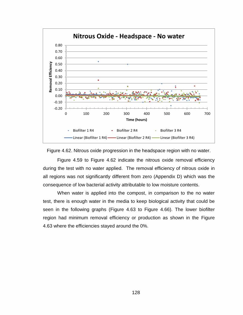
128

Figure 4.62. Nitrous oxide progression in the headspace region with no water.

Figure 4.59 to Figure 4.62 indicate the nitrous oxide removal efficiency

during the test with no water applied. The removal efficiency of nitrous oxide in

all regions was not significantly different from zero (Appendix D) which was the

consequence of low bacterial activity attributable to low moisture contents.

When water is applied into the compost, in comparison to the no water

test, there is enough water in the media to keep biological activity that could be

seen in the following graphs (Figure 4.63 to Figure 4.66). The lower biofilter

region had minimum removal efficiency or production as shown in the Figure

4.63 where the efficiencies stayed around the 0%.

-0.20

-0.10

0.00

0.10

0.20

0.30

0.40

0.50

0.60

0.70

0.80

0 100 200 300 400 500 600 700

Re

mo

val E

ffic

ien

cy

Time (hours)

Nitrous Oxide - Headspace - No water



129

Figure 4.63. Nitrous oxide removal efficiency in the lower region with water.

As in the ammonia analysis, negative values of nitrous oxide means

generation of nitrous oxide and positive values means removal. In the middle

biofilter region (Figure 4.64) nitrous oxide was generated. Some nitrous oxide

generation occurred in biofilter 2 with further removal after around 100 hours.

Biofilters 1 and 3 indicated little or no activity.

-0.4

-0.2

0.0

0.2

0.4

0.6

0.8

0 100 200 300 400 500 600 700 800

Mo

istu

re C

on

ten

t an

d N

Itro

us

Oxi

de

Re

mo

val

Time (hours)

Nitrous Oxide - Lower - With water


Media MC 1 Media MC 2 Media MC 3

Log. (BiofilterW 2 R1) Linear (BiofilterW 2 R1) Linear (BiofilterW 3 R1)

Poly. (Media MC 2) Log. (Media MC 3) Poly. (Media MC 3)

130

Figure 4.64. Nitrous oxide removal efficiency in the middle region with water.

Figure 4.65 shows that in the upper biofilter region, some nitrous oxide

was generated. This likely occurred because its moisture content was maintained

at levels above 43% for a sufficient time for the denitrifying bacteria population to

grow.

-0.4

-0.2

0.0

0.2

0.4

0.6

0.8

0 100 200 300 400 500 600 700 800

Mo

istu

re C

on

ten

t an

d N

Itro

us

Oxi

de

Re

mo

val

Time (hours)

Nitrous Oxide - Middle - With water



Poly. (BiofilterW 1 R2) Poly. (BiofilterW 2 R2) Linear (BiofilterW 3 R2)


131

Figure 4.65. Nitrous oxide removal efficiency in the upper region with water.

The biofilter media between the upper sampling port and the headspace

port indicated removal of nitrous oxide that was formed in the upper region

(Figure 4.66).

-0.4

-0.2

0.0

0.2

0.4

0.6

0.8

0 100 200 300 400 500 600 700 800

Mo

istu

re C

on

ten

t an

d N

itro

us

Oxi

de

Re

mo

val

Time (hours)

Nitrous Oxide - Upper - With water



Poly. (BiofilterW 1 R3) Poly. (BiofilterW 2 R3) Poly. (BiofilterW 3 R3)

Poly. (Media MC 1 R3) Linear (Media MC 2 R3) Linear (Media MC 3 R3)

132

Figure 4.66. Nitrous oxide removal efficiency in the upper region with water.

One very important observation can be made by considering that the

overall nitrous oxide removal efficiency remained close to 0% (Figure 4.67). If

only the overall efficiency were taken into consideration, it would have masked all

the activity which occurred in the middle of the biofilter, thus leading to an

incorrect conclusion that no nitrous oxide was generated. It was generated and

consumed (Appendix D).

-0.40

-0.30

-0.20

-0.10

0.00

0.10

0.20

0.30

0.40

0 100 200 300 400 500 600 700 800

Re

mo

val E

ffic

ien

cy

Time (hours)

Nitrous Oxide - Headspace - With water

BiofilterW 1 R4 BiofilterW 2 R4

133

Figure 4.67. Nitrous oxide removal efficiency in the overall biofilter with water.

-0.50

-0.40

-0.30

-0.20

-0.10

0.00

0.10

0.20

0.30

0.40

0.50

0 100 200 300 400 500 600 700

Re

mo

val E

ffic

ien

cy

Time (hours)

Overall Removal Efficiency

BiofilterW 1 BiofilterW 2 BiofilterW 3

Linear (BiofilterW 1) Linear (BiofilterW 2) Linear (BiofilterW 3)

134

Chapter 5 Conclusions

Three compost biofilter chambers located in the Air Quality Laboratory at

the Biosystems and Agricultural Engineering Department were evaluated for

structural integrity and uniformity. These analyses were performed to verify the

unusual behavior of biofilter number 3.

The flow meters located in the back of the biofilters were tested

individually. They were found to have a linear relation between 20 and 40 ml/min

when they were connected to a pump. The linear relation was extended from 20

to 50 ml/min when they were connected to a pressurized tank. This range

included the flow that was used during the experiments.

No major leakage in the structure of any of the biofilters was found during

the evaluation, and thus, this hypothesis was eliminated as the source of the

anomaly associated with any biofilter chamber. A small leak was identified in

between the box and the cone at one corner on biofilter #3 and also under

biofilter #1, but it could not be identified as the reason for the disparate behavior

of biofilter 3.

Evaluation of the exhaust system for any interference revealed that the

exhaust in biofilter 3 exhibited a small back pressure which caused chaotic

behavior of the smoke coming out of the biofilter. But after consideration it was

concluded that this had no effect on the contradictory values for biofilter number

3 because the back pressure and the chaotic behavior of the smoke occurred

outside of the chamber.

The air supply system was also evaluated by testing the exhaust duct

located above the plenum. It was concluded that this exhaust duct was

responsible for an unbalanced air delivery to the biofilters. When the balancing

damper was opened biofilter 1 was significantly different from the other two, and

when it was closed all three biofilters were subjected to an air flow with no

significant difference between each other.

The add-on component to the sieve shaker machine resulted in a much

better performance both in quantity of compost sieved and labor demand. It was

possible to sieve more compost with less manual labor at a faster throughput.

135

The original design demanded 25 hours of work to sieve 0.75 m3 and with the

add-on this time was reduced to 2.75 hours of work.

Compost from the Animal Research Center at the University of Kentucky

was characterized according to its physical properties and was sieved to obtain a

medium particle size ranging from 4.75 to 8 mm. This particle size represented

13% of the as received compost, and the rest of the compost was characterized

as rocks (>12.5 mm) with 3% of the total, large particle size (between 12.5 and 8

mm) with 8%, small particle size (between 4.75 and 1.35 mm) with 27% and the

fines (<1.35 mm) that represented 49% of the as received compost.

An alternative indirect method of moisture sensing was incorporated which

relied on the thermal conductivity of the compost. A relationship with an R2 of

0.925 was found for moisture content and thermal conductivity. An equation for

calculating the moisture content of compost with the thermal readings was

calculated and used during the experiment. The downside of this technology is

the need for better performance of the sensor. The probe should be completely

inserted into the mass of compost or even embedded within it. Another significant

factor is the relatively high price of the sensor.

Commercially available soaker hoses were calibrated to determine flow as

a function of pressure in order to determine the amount of water being applied to

the biofilter. A linear regression was created, to calculate the amount of water to

be applied to the compost. The water was turned on at constant pressure for a

controlled water application. The optimized position of soaker hose for water

application was the lower region of the biofilter. This was concluded because the

hose in the lower position maintained constant moisture content in the biofilter

media.

A water application interval was tested to verify if the interval that the

water was turned on and off affected the capacity of the biofilter to hold water or

drain before being adsorbed. The Tukey means grouping showed that there was

no significant difference between the intervals tested. However, the interval

where the water was allowed to run for 30 seconds with a two minute interval

between applications was different from the other two. This is an important

136

consideration for a control system design where the software controls how many

30 seconds applications will be necessary and automatically adjusting the

interval between them as may be required to maintain given moisture content.

The results of the procedures conducted during these tests indicated that further

testing was required in order to make a determination of the application interval.

The water balance conducted during the experiment showed that the no

water treatment resulted in the compost moisture content behaving as expected

where the lower region dried faster than the others reaching an equilibrium

moisture content of 10% wb at 100 hours. The middle region reached this level at

300 hours and the upper region reached a level below 20% w.b. after 400 hours.

This level of moisture content is important because it determines when the

biological activity ceases. With no water being applied to the media, the biofilter

loses its biological activity after 400 hours.

The installation of the soaker hose prevented the biofilter from dropping to

moisture content levels below 20% w.b.. The average moisture content

throughout the entire biofilter stayed above 30% w.b. Therefore, the water being

applied to the lower region of the biofilter resulted in all regions maintaining

sufficient moisture content to support biological activity.

The results reported above are based on the direct method for measuring

water content. Some measurement discrepancies with the direct method

occurred when the INNOVA was used for estimating the water in the biofilter.

Using the INNOVA measurements of the water content of the exhaust air, the

total amount of water lost was 91 kg of water when no water was applied and

308 kg of water when water was being applied. The difference in these values

demonstrates that maintaining the biofilter media moisture content requires

significant application of water.

Thermal conductance was used to track the moisture in the compost

during the experiment. The results of the analysis did not show a close

correlation between the predicted replacement volume of water and what was

actually leaving the system. The water calculated to be added into the biofilter

was lower than what was actually being lost through drying. The reason for this

137

phenomenon is still unknown and requires further study. The effect of depths of

the probe in the compost did not show any major effect in the reading that would

cause this much offset in the moisture readings. Thermal conductance for

moisture measurement was a viable indirect method for a second/control system

for water application. An alternative is to use the probes totally embedded into

the mass of compost on each of the regions of the biofilter connected with a

multiplexer for a complete moisture profile of the media.

Gas removal analysis should be performed on a region by region basis

instead of only at the inlet and outlet of the entire biofilter. The results showed

that it was possible to draw different conclusions based on these two different

analyses. In this research effort, the two treatments (no water being applied and

water being applied) had the same results when the gases were analyzed over

the entire biofilter, but when the region by region analysis was performed the

results presented different patterns.

138

Chapter 6 Recommendations for future work

Pilot scale biofilters need an impermeable finish to deal with the amount of

water that would be present during a long term experiment, or perhaps be

constructed of a different material such as a stainless-steel that would be inert to

the ammonia and standing water.

An improved, real-time water balance is important for validation of media

bed moisture content and the true effect of water application measurements and

the effects of applied water. A collector system for drainage water below the

biofilter is recommended for accounting all water losses.

Simplify the design of the air delivery system, eliminating any exhaust duct

or balancing damper for airflow regulation. This balance damper was found to be

the cause of chamber performance anomalies in earlier work.

The drying tests showed that the middle and upper regions began to dry

after the lower region was in equilibrium with the incoming gas stream. This

suggests that the lower region works as a moisture buffer for the rest of the

biofilter stacks. This characteristic function, other experiments could evaluate

using materials with different water holding capacities for the buffer region and

determine the effect on the water content in the biofilter. This modification could

also be applied to the upper region which still dries even with the middle region

being kept constant. It may be beneficial to place a buffer material over the

surface of the biofilter in order to decrease upper region drying.

Moisture sensing systems will likely require the thermal conductor to be

totally embedded in the mass of compost. Further, a multiplexer system similar to

that developed by Del Nero Maia (2010) can be adapted for the continuous

monitoring of the moisture content.

139

Appendices

Appendix A. Evaluation of capacitance as moisture measure method

A.1 Introduction

To fulfill the objective of finding an indirect nondestructive method for

moisture measurement of the compost, capacitance was evaluated as matter for

indirect measurement method for moisture content. This electrical property is

already used in different fields to this end, like in soil which have similar

characteristics to compost. And these similarities lead to the experimentation of

capacitance.

A.2 Literature Review

Capacitance is the measurement of the stored electrical charge between

parallel bodies, when there is an electrical potential and infinite resistance

between them (Kelleners et al., 2004). The technique of using capacitance for

moisture content measurement in soil have been improved substantially

(Polyakov, 2005), and present some advantages for this kind of use because is a

fast and nondestructive method for moisture measurement, also is easily

automated (Kelleners et al., 2004).

Typically to measure the moisture content in soil the probes used to

measure the capacitance operates at a wide frequency range from 10 MHz to

several hundred megahertz (Eller, 1995), these probes are a safe, fast and

inexpensive part of the capacitance method and initially they used empirical

calibrations where the probe response is directly related to the moisture content

in soil which means that the calibration is instrument dependent, to avoid this

disadvantage a twofold calibration strategy is developed and described by

Robinson et al, 1998. Because of time restraints this kind of experimentation was

not performed during this experiment.

In these tests it was used 3 control boards built by Robert et al, 2005

which were designed to work with a large area capacitive plate sensor at media

moisture content of 10 to 70% wet basis. The frequencies used were between

300 kHz to 15 MHz, with a new compost media with various particle sizes,

resulting in porosity of 57%; this media is similar to the ones used in newly

140

contracted biofilter. The experimented consisted in air drying the compost and

adding water in seven incremental steps in order to have seven different

moisture contents, for which samples were taken for drying in the microwave to

measure the moisture content by weight difference and at the same time the

capacitance in the plates were recorded.

A.3 Material and Methods

This portion of the work involved evaluation of a sensor board design

developed by Robert (2005) and was intended to satisfy a portion of the

requirements for Objective 2 but due some lack of details in the testing could not

be used. There were two phases for testing the capacitance based sensor. The

first consisted of using the control board built by Robert (2005) to develop a set

of small form factor capacitance grids which were essentially two metal grids

which acted as the capacitive surfaces. The second phase was accomplished

using a commercially available capacitance meter (BK 815, BK Precision Corp.)

to measure the capacitance through the metal grids as a function of the media

water content. The grids had a surface area of 0.133 m2 and two different wire

spacing: 1.25 cm (0.5 in) and 0.625 cm (0.25 in).

A.3.1 Chicken wire test

Robert et al (2005) described capacitance plates formed from large

galvanized fence panels approximately 91.4 cm by 76.2 cm which were much too

large for use in pilot scale biofilter studies. Thus, it was necessary to develop

small form factor grids for evaluation of the sensor boards in the present

laboratory setup. A preliminary test used a 0.625 cm (0.25 in) spacing galvanized

wire grid, commonly known as chicken wire, as the capacitance grids replacing

the large capacitive grids used by Robert et al (2005). Three airtight, plastic

boxes (with 27 liters) were filled with compost of known moisture content. Each

box contained two chicken wire grids with an area of 0.133 m2 and was filled with

sieved compost (Figure A.3.1.1 and Figure A.3.1.2). A layer of compost

approximately 2.5 cm thick was placed in the bottom of the container with the first

chicken wire grid placed above it. An additional layer of compost 2.5 cm thick

141

was placed over the first grid followed by the remaining chicken wire grid to

create the capacitance volume.

Figure A.3.1.1 Installation of the grids inside the boxes.

142

Figure A.3.1.2 Boxes with the chicken wire in the compost.

The chicken wire grids were supplied with a +/- 9 volts DC current. A

prototype “breadboard” (Figure A.3.1.3) was constructed to serve as a hardwire

switch allowing selective connection of all three boards to a multimeter (Equus

3320 Auto-Ranging Digital Multimeter). During this procedure the frequency used

was no adjusted or recorded, because the boards were tested as they were

received assuming they were in adjusted in accordance with each other.

143

Figure A.3.1.3 Prototype board connected to the control boards.

Twice a day samples of compost were removed from the boxes and dried

in an oven for 24 hours at 105oC to determine the moisture content. The

multimeter voltage across the grids was recorded for comparison to the oven-

dried values.

A.3.2 Insulated grids

Analysis of the preliminary data gathered using the chicken wire grids

indicated that the bare wire grids may have actually been short circuited through

the compost media owing to its relatively high moisture content. It was decided to

construct insulated grids and repeat the tests to determine if short circuiting did,

in fact, take place in the media. Coated wire grids made of galvanized wires and

coated with vinyl were obtained from McNichols CO. (Vinylmesh, galvanized-

PVC coated, 0.2 cm wire). Two different grid spacing (1.25 cm and 0.625 cm)

were investigated as possible replacements for the chicken wire grids. The grids

used in the experiment are smaller than what is sold by the manufacturer which

required the material to be cut. The cutting process leaves the cut points

exposed affecting its insulation properties. Thus, a tray was fabricated (Figure

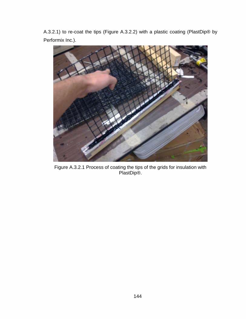
144

A.3.2.1) to re-coat the tips (Figure A.3.2.2) with a plastic coating (PlastDip® by

Performix Inc.).

Figure A.3.2.1 Process of coating the tips of the grids for insulation with PlastDip®.

145

Figure A.3.2.2 Tips of the grids insulated with PlastDip®.

The insulated grids were evaluated using two processes, dynamic and

static. Details of these processes are presented in the following sections.

A.3.2.1 Dynamic test

The grids were placed inside the biofilters (Figure A.3.2.1.1) with 68 liters

of compost at initial moisture content of 50% (w.b.). The chambers were

subjected to an airflow rate of 104 m3/h to dry the compost. The grids were

connected to separate controller boards (one for each chamber) at the same

voltage described earlier (Figure A.3.2.1.2).

146

Figure A.3.2.1.1 Grids installed in the lower position of the biofilter.

Figure A.3.2.1.2 Control board installed on the side of the biofilter.

147

The compost was allowed to dry for 12 hours. Media samples were

collected every hour for determination of the water content, along with the

voltage across the control board for later comparison. A single spacing size grid

was used in all three biofilters for each test in order to exclude the effect of

pressure drop on the drying rate. The test was repeated for both grid sizes.

The data were analyzed to determine if a relationship between moisture

content and voltage at the meter (i.e., capacitance across the grids) exists.

Linear regression was used to check for linearity of the results and analysis of

variance will be used to determine goodness of fit for the prediction model.

A.3.2.2 Static tests

The dynamic tests were designed to evaluate the sensor’s ability to track

varying moisture content over time. A subsequent set of tests referred to in this

case as static tests were designed to evaluate the sensor’s stability in measuring

relatively constant moisture content.

The static tests utilized the same plastic, airtight containers used for the

earlier chicken wire tests. Six boxes were filled with compost at known moisture

contents (40, 50 and 60% w.b.) with two grids placed 2.54 cm (1 in) apart (Figure

A.3.2.2.1). Three boxes contained the 1.27 cm (0.5 in) grid spacing and three

contained the 0.635 cm (0.25 in) grid spacing. The boxes were sealed so the

compost would not loose water with time.

148

Figure A.3.2.2.1 Boxes with the grids used for the static tests.

The static tests were performed using a commercially available

capacitance meter (BK 815, BK Precision Corp.), because the control boards

were suspected to be unstable. The readings were taken every hour for 12

hours, after which, the boxes were emptied and filled with the next moisture

content. The tests were replicated three times in order to allow every box be filled

with each of the three moisture contents.

The data were analyzed for three replicates of three moisture contents

and two grid spacing to determine if a relationship between moisture content and

capacitance at the meter exists. Linear regression was used to check for linearity

of the results and analysis of variance will be used to determine goodness of fit

for the prediction model.

A.4 Results and discussion

A.4.1 Chicken wire test

The development of a good set of small form factor capacitance plates

was undertaken as part of the requirements of objective 2 and was a

fundamental requirement to make the control boards built at the University of

149

Illinois work with the pilot scale biofilters. The design requirements included low

pressure drop, a good surface for capacitance, and economy. Chicken wire was

used in the preliminary tests of the control boards owing to its economy and

availability as an easy resource found in a farm. Its electrical capability was

tested in order to find if it would work as a set of capacitance plates.

During this test the moisture content was kept constant inside a sealed

box and the voltage read with each control board. Figure A.4.1.1 shows that for

the three control boards there is a very weak linear regression, with R2s not

bigger than 0.47, between the moisture content and the voltage. The interaction

between the boards and the moisture content has some strength with a p-value

of 0.006 what is a small p-value but with potential (Figure A.4.1.2).

Figure A.4.1.1 DC Voltage across the boards using chicken wire as capacitance plates.

y = -3.8x + 2.1 R² = 0.38

y = -1.1x + 0.9 R² = 0.26

y = -6.1x + 2.9 R² = 0.47 0

0.2

0.4

0.6

0.8

1

1.2

1.4

1.6

1.8

25% 27% 29% 31% 33% 35%

DC

Vo

ltag

e (

volt

s)


Chicken wire as capacitance plates

Board 13

Board 14

Board 15

Linear (Board 13)

Linear (Board 14)

Linear (Board 15)

150

Figure A.4.1.2 SAS output to the chicken wire tests.

One problem with the chicken wire is that they are not insulated what

would culminate in short circuiting in the compost. Capacitance is the ability of a

body to hold an electrical charge, in this case the chicken wire grids, so if the

chicken wires are short-circuiting there will be current across the compost

masking the measurements of the capacitance and also because of the compost

depending on the moisture content can work as conductor and build up electrical

charge on it.

A.4.2 Insulated grids: Dynamic Test

Insulated grids were used to avoid short-circuiting across the compost

which would directly affect the capacitance. Dynamic tests were performed by

placing the insulated grids into the biofilters during a drying test. Samples were

taken every hour and the voltage across the control boards measured. The

results of this analysis are presented in Figure A.4.2.1. Is possible to see that the

relation between moisture content and the voltage is relatively constant, like is

shown in Figure A.4.2.2 where the curves for the three boards are not

151

significantly different from each other and also not different from slope zero,

which indicates that no matter the moisture content in the compost the voltage

readings does not change.

Figure A.4.2.1 DC voltage measured on the control boards during the dynamic test with the 1.27 cm (0.5 in) insulated grids.

y = -0.36x + 1.7 R² = 0.01

y = 0.54x + 1.0 R² = 0.44

y = 0.74x + 1.2 R² = 0.39 0.75

1.25

1.75

2.25

2.75

3.25

5% 15% 25% 35% 45% 55% 65%

DC

Vo

ltag

e (

volt

s)


Voltage on 1.27 cm grids

Board 13

Board 14

Board 15

Linear (Board 13)

Linear (Board 14)

Linear (Board 15)

152

Figure A.4.2.2 SAS output to the insulated grids with wire spacing of 1.27 cm (0.5 in).

The 1.27 cm insulated grids presented very poor linear regressions with

R2s not bigger than 0.44 and all the three control boards presented regressions

that have small coefficients turning them in almost horizontal lines what means

that the voltage across the grids measured with the control board does not vary

with the moisture content of the compost. The 0.635 cm (0.25 in) grids also

presented similar behavior in what concerns the voltage across the grids with the

moisture content (Figure A.4.2.3) with linear regression approximating of

horizontal lines, which can be inferred by analyzing the p-values in Figure A.2.4

showing that the slopes are not significantly different from each other or to the

zero slope. The results showing horizontal lines mean that the voltage does not

change with the moisture content.

153

Figure A.4.2.3 DC voltage measured on the control boards during the dynamic test with the 0.635 cm (0.25 in) insulated grids.

y = -0.11x + 1.0 R² = 0.20

y = 0.48x + 1.2 R² = 0.35

y = 0.34x + 0.51 R² = 0.02 0.6

0.8

1

1.2

1.4

1.6

1.8

40% 45% 50% 55% 60% 65% 70% 75%

DC

Vo

ltag

e (

volt

s)


Voltage on 0.635 cm grids

Board 13

Board 14

Board 15

Linear (Board 13)

Linear (Board 14)

Linear (Board 15)

154

Figure A.4.2.4 SAS output to the insulated grids with wire spacing of 0.635 cm (0.25 in).

A.4.3 Insulated grids: Static Test

Static tests were also performed with these insulated grids, this series of

tests involved placing the grids into a compost box in which the moisture content

was more or less constant and measuring the capacitance across the grids. It

was expected that this measurement would be stable because of the association

of the capacitance with the moisture content.

Graphic representations of the capacitance readings for different moisture

contents and the two grids spacing are presented in the Figure A.4.3.1 to Figure

A.4.3.6.

155

Figure A.4.3.1 Capacitances across the 1.27 cm (0.5 in) grids when moisture

content is 40% w.b.

Figure A.4.3.2 Capacitances across the 1.27 cm (0.5 in) grids when moisture content is 50% w.b.

y = 0.2713x + 13.241 R² = 0.8259

y = -0.3636x + 54 R² = 0.0394

y = 1.1105x + 13.642 R² = 0.6511 0

10

20

30

40

50

60

70

0 2 4 6 8 10 12

Cap

acit

ance

(m

F)

Time (hours)

40% moisture content

Day 1

Day 2

Day 3

Linear (Day 1)

Linear (Day 2)

Linear (Day 3)

y = 0.2014x + 11.726 R² = 0.8278

y = -0.8664x + 28.615 R² = 0.6643

y = 0.6822x + 13.49 R² = 0.9211 0

5

10

15

20

25

30

35

0 2 4 6 8 10 12

Cap

acit

ance

(m

F)

Time (hours)

50% moisture content (1.27 cm)

Day 1

Day 2

Day 3

Linear (Day 1)

Linear (Day 2)

Linear (Day 3)

156


content is 60% w.b.


content is 40% w.b.

y = 0.20x + 8.1 R² = 0.83

y = 0.40x + 12.3 R² = 0.77

y = 6.05x + 15.4 R² = 0.90

0

10

20

30

40

50

60

70

80

90

0 2 4 6 8 10 12

Cap

acit

ance

(m

F)

Time (hours)


Day 1

Day 2

Day 3

Linear (Day 1)

Linear (Day 2)

Linear (Day 3)

y = -0.57x + 64.7 R² = 0.26

y = -0.68x + 82.5 R² = 0.34

0

10

20

30

40

50

60

70

80

90

100

0 2 4 6 8 10 12

Cap

acit

ance

(m

F)

Time (hours)


Day 1

Day 2

Linear (Day 1)

Linear (Day 2)

157

Figure A.4.3.5 Capacitances across the 0.635 cm (0.25 in) grids when moisture content is 50% w.b.


content is 60% w.b.

y = 0.29x + 9.8 R² = 0.74

y = -0.24x + 15.8 R² = 0.53

0

2

4

6

8

10

12

14

16

18

0 2 4 6 8 10 12

Cap

acit

ance

(m

F)

Time (hours)


Day 1

Day 2

Linear (Day 1)

Linear (Day 2)

y = 0.29x + 9.8 R² = 0.74

y = -0.19x + 15.4 R² = 0.28

0

2

4

6

8

10

12

14

16

18

0 2 4 6 8 10 12

Cap

acit

ance

(m

F)

Time (hours)


Day 1

Day 2

Linear (Day 1)

Linear (Day 2)

158

These graphic representations of the capacitance being tested with

constant moisture showed that the capacitance was changing over time. Some of

the regressions have larges R2’s what means good fit for the period of the

experiment. But during the experiment the observations was that the number

were constantly increasing. This behavior can be associated to the use of DC

voltage during the experiment which can lead to the accumulation of charge in

the compost.

To verify this behavior where the capacitance increases with time, a

further test was performed with the same boxes with the moisture sealed to keep

constant over time. So the capacitance was measured every hour for 12 hours

for five days. Figure A.4.3.7 shows the capacitance readings for 6 different

moisture levels with the 1.27 cm (0.5 in), a Pearson correlation analysis (Table

A.4.3.1) were performed to verify the correlation of the capacitance with time that

showed a very strong correlation.

Figure A.4.3.7 Insulated grids capacitance readings for DC voltage excitation for different moisture contents.

0

5

10

15

20

25

30

35

0 20 40 60 80 100 120 140 160

Cap

acit

ance

(m

F)

Time (hours)

Insulated Grids

10%

45%

30%

35%

40%

50%

159

Table A.4.3.1 Correlation of capacitance with time.

Pearson Correlation Coefficients, N = 162 Prob > |r| under H0: Rho=0

Time logcap

Time

1.00000

-0.31154 <.0001

logcap

-0.31154 <.0001

1.00000

A.5 Conclusions

Although these experimentations were not conclusive about the capability

of the capacitance as an method for moisture content measurement, because

during this experiment the frequency was not adjusted, also it was not used the

AC current, is important to point out that the insulated wire grids are an

interesting approach for future works when evaluating the capacitance in the

compost media. Also from these tests is possible to take the correct protocol to

test, where the compost stays at constant moisture content and the capacitance

is recorded over time for further correlation.

160

Appendix B. Statistical Analysis for Flow meters tests

Table B.1 Annova for the flow meters connected to the pump through the mass

flow controller.

Anova: Single Factor

SUMMARY Groups Count Sum Average Variance

FM3 7 223 31.85714 384.8095 FM2 7 215 30.71429 374.9048 FM1 7 186 26.57143 196.9524

ANOVA Source of Variation SS df MS F P-value F crit

Between Groups 108.2857 2 54.14286 0.169786 0.845181 3.554557

Within Groups 5740 18 318.8889

Total 5848.286 20

Table B.2 Annova for the flow meters connected to the pump through the mass

flow controller in the reduced operation range for the research.

Anova: Single Factor


FM3 5 113 22.6 189.8 FM2 5 107 21.4 164.8 FM1 5 106 21.2 169.2

ANOVA Source of

Variation SS df MS F P-value F crit

Between Groups 5.733333 2 2.866667 0.016418 0.983738 3.885294

Within Groups 2095.2 12 174.6

Total 2100.933 14

161

Table B.3 Annova for the flow meters connected in series with the pump using

the mass flow controller with a flow of 20 ml/min.

Flow meters connected in series with the pump

MFC 20

SUMMARY

Groups Count Sum Average Variance

1 3 7.3 2.4 0.4

2 3 9.5 3.2 1.6

3 3 10 3.3 0.6

ANOVA

Source of Variation SS df MS F P-

value F

crit

Between Groups 1.4 2 0.7 0.8 0.49 5.1


Total 6.4 8

Table B.4 Annova for the flow meters connected in series with the pump using

the mass flow controller with a flow of 20 ml/min.

Flow meters connected in series with the pump

MFC 25

SUMMARY


1 3 18.0 6.0 3.3

2 3 23.5 7.8 5.1

3 3 24.5 8.2 0.6

ANOVA

Source of Variation SS df MS F P-

value F

crit

Between Groups 8.2 2 4.1 1.4 0.32 5.1


Total 26 8

162

Table B.5 Annova for the flow meters connected to the tank through the mass

flow controller.

Flow meters conected to the air cylinder through MFC

SUMMARY


FM3 7 289 41.3 103.2

FM2 7 286 40.9 89.2

FM1 7 278 39.7 107.2

ANOVA

Source of Variation SS df MS F P-value F crit

Between Groups 9.2 2 4.6 0.0 0.95 3.6


Total 1807.5 20

Table B.6 Annova for the flow meters connected in series with the air cylinder

using the mass flow controller with a flow of 20 ml/min.

Anova: Single Factor MFC 20


1 3 40 13.33 14.58 2 3 68 22.67 16.33 3 3 57.5 19.17 27.08


Between Groups 133.388889 2 66.69 3.45 0.10 5.14

Within Groups 116 6 19.33

Total 249.388889 8

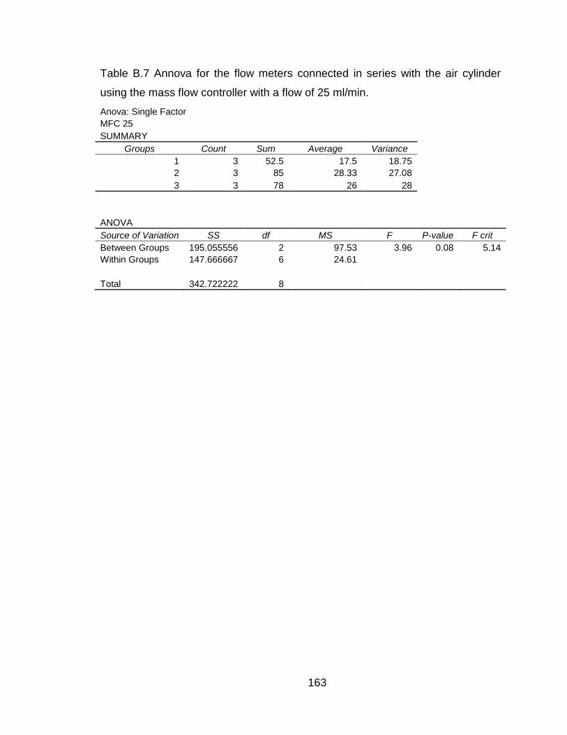
163

Table B.7 Annova for the flow meters connected in series with the air cylinder

using the mass flow controller with a flow of 25 ml/min.

Anova: Single Factor MFC 25


1 3 52.5 17.5 18.75 2 3 85 28.33 27.08 3 3 78 26 28


Between Groups 195.055556 2 97.53 3.96 0.08 5.14

Within Groups 147.666667 6 24.61

Total 342.722222 8

164

Appendix C. Statistical Analysis for the drying front movement

The drying front movement was described in order to visualize the

different drying processes that happen inside the biofilter and with these data to

show where the and if the moisture is constant when the slopes are not

significantly different from zero. Below find the SAS code for these comparisons

and the output for each of the region. Information from this analysis is the

uniformity of the biofilters as replicates.

Table C.1 SAS code used for comparing the slopes of the drying front for each of

the region in the biofilters.

The first analysis performed is the drying period on the lower region, which

happens from 0 to 52 hours. In Table C.2 is possible to see that the slopes are

different from zero but not significantly different from each other, what enforces

that the three biofilters are true replicates.

165

Table C.2 SAS output for slope analysis of the drying period in the lower region.

After the drying period starting at 52 hours the lower region gets into

equilibrium moisture content around 10% wet basis. This equilibrium can be seen

on Table C.3 where the slopes are not significantly different from zero what

means a constant slope and also not significantly different from each other.

166

Table C.3 SAS output for slope analysis of the equilibrium period in the lower

region.

In the middle region during the firsts 52 hours the moisture content stays

in equilibrium while the lower region is drying. This equilibrium period is shown in

Table C.4 whit the same output as the equilibrium period in the lower region

where the slopes are not significantly different from zero and from each other.

167

Table C.4 SAS output for slope analysis of the equilibrium period in the middle

region.

The drying period in the middle region starts after the 52 hours period

which is proved in the Table C.5 with the slopes being significantly different from

zero. And like the other analysis the biofilters are all working uniformly.

168

Table C.5 SAS output for slope analysis of the drying period in the middle region.

As in the middle region the upper region has a constant moisture content

period and starts to dry after a point. But even though the upper part has a

similar pattern as the middle the constant moisture content period goes until 65

hours and them starts to dry, these periods of constant moisture content and

drying for the upper region are presented in Table C.6.

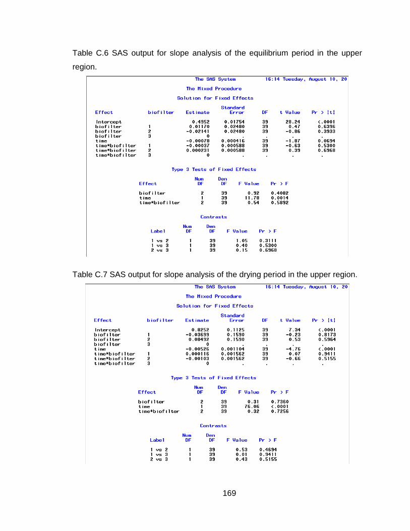
169

Table C.6 SAS output for slope analysis of the equilibrium period in the upper

region.

Table C.7 SAS output for slope analysis of the drying period in the upper region.

170

Appendix D. Nitrous Oxide Removal efficiencies Statistics

When there was no water being applied into the biofilter the nitrous oxide

generation and/or removal was not significantly different from zero, this

performance is due to the fact that the nitrous oxide can only be generated by

microbial activity and this microbial activity cannot happens on low moisture

conditions. The descriptive statistics for the slopes of removal are presented in

Table D.1, Table D.2 and Table D.3.

Table D.1 Descriptive statistics for nitrous oxide removal efficiency when no

water is being applied into the biofilter 1.

Biofilter 1 (No Water)

Lower Middle Upper Headspace Overall

Mean 0.00 0.00 -0.01 0.00 0.00

Standard Error 0.01 0.00 0.00 0.01 0.01

Median 0.00 0.00 0.00 0.00 0.00

Mode -0.01 0.00 0.00 0.00 0.00

Standard Deviation 0.07 0.06 0.06 0.07 0.08

Sample Variance 0.01 0.00 0.00 0.01 0.01

Kurtosis 47.15 38.58 56.60 33.83 45.20

Skewness 5.57 -4.33 -5.87 4.86 5.42

Range 0.83 0.64 0.65 0.70 0.86

Minimum -0.15 -0.53 -0.56 -0.16 -0.14

Maximum 0.68 0.11 0.09 0.54 0.72

Sum 0.53 -0.23 -0.87 0.69 0.12

Count 163.00 163.00 163.00 163.00 163.00

Confidence Level(95.0%) 0.01 0.01 0.01 0.01 0.01

171





Mean 0.00 0.00 0.00 0.01 0.00

Standard Error 0.01 0.01 0.01 0.00 0.00

Median 0.00 0.00 -0.01 0.01 0.00

Mode 0.00 #N/A #N/A #N/A 0.00


Sample Variance 0.01 0.01 0.01 0.00 0.00

Kurtosis 31.03 99.39 98.88 14.55 13.64

Skewness -1.51 -8.27 8.81 -0.82 2.49

Range 0.95 1.81 1.15 0.57 0.53

Minimum -0.58 -1.31 -0.15 -0.33 -0.16

Maximum 0.37 0.50 1.00 0.25 0.37

Sum -0.40 -0.36 0.19 0.85 0.27

Count 163.00 163.00 163.00 163.00 163.00






Mean 0.00 -0.01 0.01 0.00 0.00

Standard Error 0.00 0.01 0.01 0.00 0.00

Median 0.00 0.00 0.00 0.00 0.00

Mode #N/A 0.00 0.00 #N/A -0.01


Sample Variance 0.00 0.01 0.01 0.00 0.00

Kurtosis 15.99 96.02 97.17 1.12 8.73

Skewness -0.42 -8.29 8.78 0.34 1.26

Range 0.62 1.48 1.08 0.24 0.53

Minimum -0.35 -1.12 -0.12 -0.09 -0.22

Maximum 0.27 0.35 0.96 0.15 0.31

Sum -0.08 -1.35 1.27 -0.02 -0.18

Count 163.00 163.00 163.00 163.00 163.00


172

In the other hand when water is applied to the biofilter is possible to identify

some activities happening in the biofilter because now there enough water in the

biofilter to maintain biological activity. This activity can be described by the

descriptive statistics presented on Table D.4, Table D.5 and Table D.6.

Table D.4 Descriptive statistics for nitrous oxide removal efficiency when water is

being applied into the biofilter 1.

Biofilter 1 (Water)


Mean 0.01 -0.01 -0.09 0.07 -0.02

Standard Error 0.01 0.01 0.01 0.01 0.01

Median 0.02 -0.01 -0.08 0.06 -0.01

Mode #N/A #N/A #N/A #N/A #N/A


Sample Variance 0.03 0.01 0.02 0.02 0.03

Kurtosis 28.99 15.13 21.75 31.24 13.78

Skewness -2.92 1.20 -3.53 -2.32 -1.77

Range 2.01 1.33 1.36 1.87 1.77

Minimum -1.26 -0.56 -1.06 -1.09 -1.14

Maximum 0.75 0.76 0.30 0.78 0.63

Sum 1.13 -1.28 -13.05 10.10 -3.09

Count 151.00 151.00 151.00 151.00 151.00


173



Biofilter 2 (Water)


Mean -0.02 0.03 -0.10 0.07 -0.02

Standard Error 0.01 0.02 0.02 0.01 0.01

Median -0.01 0.03 -0.09 0.08 -0.01

Mode -0.01 #N/A #N/A #N/A -0.11


Sample Variance 0.01 0.04 0.04 0.03 0.03

Kurtosis 22.81 45.78 36.93 37.92 22.21

Skewness -3.36 -4.21 3.62 -4.71 -3.31

Range 1.18 2.59 2.50 1.91 1.80

Minimum -0.95 -1.69 -0.81 -1.31 -1.29

Maximum 0.23 0.91 1.70 0.60 0.51

Sum -2.84 4.31 -15.34 11.24 -2.63

Count 151.00 151.00 151.00 151.00 151.00




Biofilter 3 (Water)


Mean -0.01 0.00 -0.02 0.06 0.02

Standard Error 0.03 0.03 0.02 0.01 0.01

Median 0.02 0.00 -0.03 0.04 0.03

Mode #N/A 0.00 #N/A #N/A 0.00


Sample Variance 0.11 0.16 0.06 0.01 0.02

Kurtosis 122.11 68.51 42.63 23.63 15.01

Skewness -10.55 4.91 5.40 3.68 -1.68

Range 4.22 5.88 2.69 1.17 1.63

Minimum -3.90 -1.99 -0.76 -0.17 -0.95

Maximum 0.32 3.89 1.92 1.00 0.69

Sum -1.86 -0.49 -3.66 9.53 3.52

Count 151.00 151.00 151.00 151.00 151.00


174

Appendix E. Water replacement calculation

The water replaced during the soaker hoses positioning test was a fixed

value calculated based on a previous test of drying. In this test it would be

calculate the drying rate in kg of water lost per hour. And the biggest rate found

during this drying test would be used as reference. It was assumed that if the

hoses could deliver enough water to replace this amount, even when the drying

rates are smaller it would have the water replaced.

Table E.1 Moisture content wet base for the drying test.

Lower Middle Upper

0 48% 49% 49%

17 34% 50% 48%

41 19% 49% 47%

52 15% 44% 47%

65 9% 43% 42%

76 11% 32% 37%

89 9% 22% 37%

100 9% 16% 33%

113 8% 11% 26%

Each region of the biofilter was filled with an average of 31.2 kg of wet

compost. To transform the Table E.1 in water content is necessary to transform

the wet basis moisture content into dry basis shown in Table E.2, with the

equation E.1.

E.1

MW = moisture content (wet basis)

= moisture content (dry basis)

175

Table E.2 Moisture content dry base for the drying test.

Lower Middle Upper

0 92% 95% 94%

17 51% 98% 91%

41 23% 97% 88%

52 18% 79% 89%

65 9% 74% 71%

76 12% 47% 58%

89 9% 29% 58%

100 10% 19% 48%

113 8% 13% 35%

The initial water content among with the dry mass of the compost is

calculated by multiplying the initial moisture content wet basis by the mass of

compost. Table E.3 shows the dry mass and water content in each region.

Table E.3 Water content and dry mass content of compost in the biofilter in kg.

Lower Middle Upper

Water 15.0 15.2 15.1

Dry

Mass 16.2 16.0 16.1

The dry mass in the compost is constant during the whole experiment, what

makes it the unit used to calculate the exactly amount of water present in the

compost, the results are in Table E.4.

176

Table E.4 Water content in kg of water in each region during the drying test.

Lower Middle Upper

0 14.97 15.21 15.14

17 8.23 15.70 14.60

41 3.76 15.54 14.09

52 2.91 12.55 14.23

65 1.53 11.86 11.45

76 1.91 7.55 9.34

89 1.53 4.64 9.39

100 1.55 3.07 7.73

113 1.37 2.04 5.66

When the difference between water contents by the time of the

measurements a drying rate is found in kg of water per hour (Table E.5).

Table E.5 Drying rates for each region in kg of water per hour.

Lower Middle Upper

0 0.00 0.00 0.00

17 0.40 -0.06 0.03

41 0.19 -0.01 -0.35

52 0.08 -0.08 0.00

65 0.11 -0.01 -0.07

76 -0.03 -0.07 -0.04

89 0.03 -0.04 0.00

100 0.00 -0.02 -0.02

113 0.01 -0.01 -0.02

177

References

Swanson, W. J.; Loehr R. C.; Biofiltration: Fundamentals, Design and

Operations Principles, and Applications, Journal of Environmental Engineering,

1997; 123(6): 538-546.

Ergas, J. S.; Schroeder, E. D.; Chang, D. P. Y.; Morton, R. L.: Control fo

Volatile Organic Compound Emissions Using a Compost Biofilter. Water Environ

Res 1995, 67: 816-821.

Cohen Y.; Biofiltration - the treatment of fluid by microorganisms

immobilized into the filter bedding material: a review. Bioresource Technol, 2001;

77: 257-274.

Morales M, Hernandez S, Cornabe T, Revah S, Auria R; Effect of drying

on biofilter performance: modeling and experimental approach. Environ Sci

Technol, 2003, 37:985–992.

Devinny, J. S., M. A. Deshusses, T. S. Webster.;Biofiltration for Air

Pollution Control. Lewis Publishers, Boca Raton, FL, 1999

Bohn HL, Bohn KH; Moisture in biofilters. Environ Prog, 1999, 18:156–

161.

Cardenas-Gonzalez B, Ergas S, Switzenbaum M & Phillibert N; Evaluation

of full-scale biofilter media performance. Environ. Prog., 1999, 18: 205–211.

Sylvia, D. M., J. J Fuhrmann, P. G Hartel, and D. A. Zuberer (eds).

Principles and Applications of Soil Microbiology. Upper Saddle River, NJ:

Prentice Hall. 1998

Sharma B., Ahlert R. C.; Nitrification and nitrogen removal. Water Res,

1977, 11: 897–925

178

Mann, D.D., J.C. DeBruyn and Q. Zhang.; Design and evaluation of an

open biofilter for treatment of odour from swine barns during sub-zero ambient

temperatures. Canadian Biosystems Engineering, 2002. 44(6): 21-26.

Sales, G. T.; Assessment of Biofilter Media particle Sizes for Removing

Ammonia. M.S. Thesis; Biosystems and Agricultural Engineering, University of

Kentucky. 2008; 143pp.

Del Nero Maia, G.; Ammonia Biofiltration and Nitrous Oxide Generation as

Affected by Media Moisture Content. Doctoral Dissertation; Biosystems and

Agricultural Engineering, University of Kentucky. 2010; 269.

Smith P, et al.; Greenhouse gas mitigation in agriculture. Philos Trans R

Soc Lond B Biol Sci 363:789–813, 2008.

Baquerizo, G, et. al.; A detailed model of a biofilter for ammonia removal:

Model parameters analysis and model validation, Chemical Engineering Journal,

Volume 113, Issues 2-3, Selected papers from the USC-CSC-TRG Biofiltration

Conference, October 2004, 20 October 2005, Pages 205-214.

Boyette, A.R. (1998) Getting Down to (Biofilter) Basics. BioCycle, 39, 5, 58

Wani. A, Branion, R., A.; Effects of periods of starvation and fluctuating

hydrogen sulfide concentration on biofilter dynamics and performance, Journal of

Hazardous Materials, Volume 60, Issue 3, July 1998, Pages 287-303.

Tchobanoglous G, Burton FL. 1991. Wastewater engineering: Treatment,

disposal, and reuse. New York, NY: McGraw-Hill, Inc. 1334 p.

Vovelle, C.; Pollutants from Combustion—Formation and Impact on

Atmospheric Chemistry (Kluwer, Dordrecht, 2000).

Environment Protection Agency; An Introduction to Indoor Air Quality

(IAQ), Volatile Organic Compounds (VOCs); Technical Overview, 2010.

179

Saliling, W., Westerman, P., Losordo, T.; Wood chips and wheat straw as

alternative biofilter media for denitrification reactors treating aquaculture and

other wastewaters with high nitrate concentrations, Aquacultural Engineering,

Volume 37, Issue 3, November 2007, Pages 222-233.

Green, A. R., G. A. Watkins, G. B. Day, J. R. Barnett, and R. S. Gates.

2005. Design of a biofilter for swine waste facility. In Seventh International

Livestock Environment Symposium ,eds. T. Brown-Brandl and R. Maghirang,

350-357. St. Joseph, Mich.: ASABE.

Robert, M. J., T. L. Funk, J. M. Appleford, and Y. Chen. 2005. Moisture

sensing methods for biofilters treating exhaust air from livestock buildings.

ASABE paper no. 054051. St. Joseph, MI: ASABE.

Nicolai, R.E., K.A. Janni, L.D. Jacobson, and D.R. Schmidt. 1999. Biofilter

Demonstration Project. Final report prepared for the Minnesota Department of

Agriculture and the Minnesota Agricultural Experiment Station. Department of

Biosystems and Agricultural Engineering, University of Minnesota, St. Paul, MN.

Goldstein EJC, Citron DM, Nesbit CA.; Diabetic foot infections.

Bacteriology and activity of 10 oral antimicrobials agents against bacteria isolated

from consecutive cases. Diabetes Care 1996; 19: 638 – 641.

Kelleners, T.J., R.W.O. Soppe, D.A. Robinson, M.G. Schaap, J.E. Ayars,

and T.H. Skaggs. 1004a. Calibration of capacitance probe sensors using electric

circuit theory. Soil Sci. Soc.Am.J. 68: 430 – 439.

http://www.sciencedirect.com/science/article/pii/S0065211306900029-

bbib0057 Polyakov, V.O.; Fares, A. and Ryder, M.H.; Calibration of a

capacitance system for measuring water content of tropical soil, Vadoze Zone J.

4 (2005), pp. 1004–1010.

DeWitt I.; Fundamentals of Heat and Mass Transfer, New York: Wiley,

1996.

180

Chandrakanthi et al., M. Chandrakanthi, A.K. Mehrotra and J.P.A.

Hettiaratchi, Thermal conductivity of leaf compost used in biofilters: an

experimental and theoretical investigation, Environmental Pollution 136 (2005),

pp. 167–174.

Lashof, D. A., Ahuja D. R.; Relative contributions of greenhouse gas

emissions to global warming; Natural Resources Defense Council, Washington

DC, USA; Tata Energy Research Institute, New Delhi, India; Nature – Vol 344,

1990.

Ahn, H.K., Sauer, T.J., Richard, T.L., Glanville, T.D.; Determination of thermal

properties of composting bulking materials; ScienceDirect Elsevier; Biosource

Technology 100 (3974-3981), 2009.

http://www.sciencedirect.com/science/article/pii/S0960852409002697#bbib8

181

Vita

Lucas Dutra de Melo

Education

High School Associate Degree

Business and Management, by the Technological School of Management (1999-2002)

Higher Education

Environmental and Agricultural Engineering, Federal University of Viçosa, Viçosa – Brazil (2003-2008)

Biosystems and Agriculture Engineering, Iowa State University (2007)

Languages

English

Spanish (reads and writes)

Portuguese

Computing and Software

Corel Draw®

AutoCad®

Windows® and Linux

Pacote Office® and OpenOffice

Matlab® and SAS®

Professional Experience

2009-2011 Research Assistant in the Air Quality Laboratory at Biosystems and Agricultural Engineering Department of University of Kentucky

2008 Internship in ARCA (Regional Association of Coffee Producers) for evaluation of different drying methods for quality coffee

2007 Internship in Grain Quality Laboratory at Iowa State University

2007 Internship at Agrijunior in the project of an Economic Evaluation of a Micro Hydroelectrically Central at Ponte Alta Farm, Brazil

2007 Study Exchange program for Biosystems and Agricultural Engineering in Iowa State University, USA

2005/2006 Undergrad Scientific Initiation by PIBIC/CNPq in Development of a Furnace for Agricultural Products Drying

2005 Undergrad Scientific Initiation in Evaluation of Eucalypt Briquettes as fuel in a Gasifier for Agricultural Products Drying

182

2005 Undergrad Scientific Initiation in the Development of a Gasifier for Agricultural Products Drying

2004 Director of Marketing in Agrijunior (Junior Company for Students of Environmental and Agricultural Engineering)

Extra-Curricular Courses

Brazil Entrepreneurship from SEBRAE (2000)

Learning Entrepreneurship from SEBRAE (2001)

Management of Grain Elevators from CENTREINAR (2005)

Grain Handling from CENTREINAR (2006)

Development and Use of Macros in EXCEL ® (2006)

Irrigation Systems Management (2007)

AutoCad® 2 and 3D (2007)

Grain Classification from CENTREINAR (2007)

Small Dams Designs (2008)

Congress and Seminars

ASABE Annual International Meeting (2011)

ASABE Annual International Meeting (2010)

XXXVII Brazilian Congress of Agricultural Engineers (2008)

I Student Congress of UFV (2007)

IV International Seminar of Precision Agriculture (2007)

Workshop of Use and Reuse of Water – Salt and Waste Water (2007)

XXXVI Brazilian Congress of Agricultural Engineers (2007)

I Meeting of Coffee Producers of the Matas de Minas, II Workshop of Special Coffees from Minas Hills and V Meeting of Evaluation of Technic of Pro-Coffee

Forum Mineiro of Management, Muriaé (2005)

IV Seminar of Grain Storage, Uberlândia (2005)

Documents

MOISTURE CONTROL METHODOLOGY FOR GAS PHASE …