MODULE TITLE : CONTROL SYSTEMS AND AUTOMATION TOPIC … · LESSON 2 : VALVE POSITIONERS AND VALVE SIZING CSA - 4 - 2 ... the pivot point of the force balance bar. This allows the

MODULE TITLE : CONTROL SYSTEMS AND AUTOMATION

TOPIC TITLE : CONTROL DEVICES AND SYSTEMS

LESSON 2 : VALVE POSITIONERS AND VALVE SIZING

CSA - 4 - 2

© Teesside University 2011

Published by Teesside University Open Learning (Engineering)

School of Science & Engineering

Teesside University

Tees Valley, UK

TS1 3BA

+44 (0)1642 342740

All rights reserved. No part of this publication may be reproduced, stored in a

retrieval system, or transmitted, in any form or by any means, electronic, mechanical,

photocopying, recording or otherwise without the prior permission

of the Copyright owner.

This book is sold subject to the condition that it shall not, by way of trade or

otherwise, be lent, re-sold, hired out or otherwise circulated without the publisher's

prior consent in any form of binding or cover other than that in which it is

published and without a similar condition including this

condition being imposed on the subsequent purchaser.

________________________________________________________________________________________

INTRODUCTION________________________________________________________________________________________

In many control applications the need for accurate response and positioning of

the valve opening dictates the use of valve positioners. This lesson describes

the construction and operation of valve positioners and also deals with the

"sizing" of control valves.

________________________________________________________________________________________

YOUR AIMS________________________________________________________________________________________

On completion of this lesson you should be able to:

• state the reasons for using a valve positioner

• sketch and explain the operation of a typical valve positioner

• explain how reverse action and split range operation is achieved in a

valve positioner

• define flow coefficient and explain its use in determining the sizes of

control valves on liquid duties

• explain how noise, flashing and cavitation are created in control

valves

• describe the problems they cause and how their effects can be

minimised.

1

Teesside University Open Learning(Engineering)


________________________________________________________________________________________

REASONS FOR USING A VALVE POSITIONER________________________________________________________________________________________

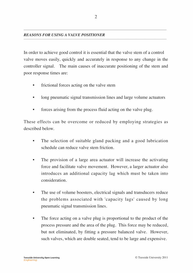
In order to achieve good control it is essential that the valve stem of a control

valve moves easily, quickly and accurately in response to any change in the

controller signal. The main causes of inaccurate positioning of the stem and

poor response times are:

• frictional forces acting on the valve stem

• long pneumatic signal transmission lines and large volume actuators

• forces arising from the process fluid acting on the valve plug.

These effects can be overcome or reduced by employing strategies as

described below.

• The selection of suitable gland packing and a good lubrication

schedule can reduce valve stem friction.

• The provision of a large area actuator will increase the activating

force and facilitate valve movement. However, a larger actuator also

introduces an additional capacity lag which must be taken into

consideration.

• The use of volume boosters, electrical signals and transducers reduce

the problems associated with 'capacity lags' caused by long

pneumatic signal transmission lines.

• The force acting on a valve plug is proportional to the product of the

process pressure and the area of the plug. This force may be reduced,

but not eliminated, by fitting a pressure balanced valve. However,

such valves, which are double seated, tend to be large and expensive.

2



An effective method of improving valve performance involves the

employment of a valve positioner. Essentially, this forms a high gain closed

loop system centred on the control valve. The positioner can be designed as an

integral part of the valve actuator or can be mounted directly on the valve

itself.

A valve positioner accurately monitors the actual valve stem position,

compares it to the desired position as indicated by the signal from the

controller, then adjusts the valve actuator pressure accordingly. FIGURE 1(a)

shows the schematic arrangement of a valve positioner which is mounted

directly on a control valve. FIGURE 1(b) shows the valve positioner and

control valve represented in block diagram form.

FIG. 1(a)

Output to valve

Controlleroutputsignal

Bellows Actuator

Valvespindle

Valvebody

Force balance bar

Pivot

Flappernozzle

Airsupply

Directacting

pneumaticrelay

3



FIG. 1(b)

OPERATION OF THE VALVE POSITIONER

An increase in controller signal expands the bellows, compresses the spring

and pushes the flapper onto the nozzle. This increases the nozzle back-

pressure and hence the output pressure from the relay. This output pressure is

fed to the valve actuator which moves the valve stem downwards.

The downward movement of the valve stem is fed back to the valve positioner

by means of the force balance bar, which pivots clockwise and further

compresses the spring. The compressed spring tends to lift the flapper away

from the nozzle, causing the nozzle back-pressure to fall and reduce the

amplified output of the relay.

This activity continues until a point of equilibrium is reached and the actual

position of the valve stem matches the desired position, as indicated by the

input signal from the controller.

The employment of feedback is the key to rapid and precise valve positioning.

Insufficient valve movement, caused, for example, by excessive stem friction,

will result in reduced spring compression and flapper 'lift'. The relay output

Nozzle &relay

Actuator& stemBellows

Valveplug

Spring Forcebar

Gainadjustment

Flappermovement

Controllersignal

Process+

–

4



pressure will remain high, allowing an increase in actuator pressure sufficient

to re-position the valve.

Alternatively, excessive valve movement will produce an increase in spring

compression and flapper 'lift', resulting in a reduced actuator pressure.

The gain of the valve positioner, which is the relationship between valve stem

travel and the change in controller input signal, can easily be varied by moving

the pivot point of the force balance bar. This allows the valve positioner to be

adapted to different types of control valve involving different ranges of stem

travel.

Cam-Type Valve Positioner

A cam-type valve positioner employs a contoured cam to transmit movement

of the valve stem to the flapper mechanism, and carries out the same function

as the positioner already described. Refer to FIGURE 2 overleaf as you read

the explanation of its operation.

5



FIG. 2

Operation of the Cam-Type Valve Positioner

The cam, which forms an essential part of the feedback mechanism, can be

designed to have a profile which will produce a required feedback relationship.

The amount of feedback determines the gain of the positioner, and hence

governs the relationship between the controller output signal and the valve

stem movement. If the cam is non-linear, the relationship between the

controller input signal and the controlled flow will also be non-linear.

Hence, by reshaping the cam it is possible to change the apparent inherent flow

characteristics of a control valve. For example, a valve positioner can be used

to convert a 'linear' valve to one having equal percentage flow characteristics.

RelayAir supply

Flapper

Nozzle Feedbackspring

Inputbellows

Inputsignal

RollerCam

Pivots

Valvestem

6



________________________________________________________________________________________

CONTROL VALVE FAIL SAFE OPERATION________________________________________________________________________________________

In selecting a control valve for a particular application, the parameters which

must be considered include those listed below.

• The force available from the actuator to position the valve.

• The size of the valve body.

• The materials of construction and the fluid being regulated.

• The flow characteristics required.

• The effect on the plant and process fluid of an air supply failure.

We have already referred to the spring of a control valve returning the valve to

a rest position, which is described as the fail safe position.

A valve which is designed to fail in the open position is called an "open air

failure valve" (OAF valve). In certain situations the terms "air to close" (ATC)

or air fail valve open (AFVO) are used.

A valve which is designed to fail in the closed position is called a "closed air

failure valve" (CAF valve). In certain situations the terms "air to open" (ATO)

or air fail valve closed (AFVC) are used.

Selection of the correct air failure action, appropriate to the particular process,

is essential to address safety issues.

FIGURE 3 shows part of a process in which a reaction vessel fluid is being

heated by means of a steam coil. Let’s look at this process to see why

selection of the correct air failure action is important.

7



FIG. 3

Valve TCV regulates the flow of steam and is activated by the controlling

instrument, TIC. If a fault develops and the instrument air supply fails, TCV

can come to rest in either the open or closed position.

If the valve fails in the open position, the steam will continue to heat the

process fluid within the vessel, which might result in the fluid reaching a

dangerously high temperature and or pressure, resulting in possible damage to

the process equipment.

Alternatively, if an air supply failure sets the valve in the closed position, the

steam supply is shut off, causing the process fluid to cool down.

TIC 1

TCV 1Steamin

Steamout

Process inflow

Processoutflow

Reaction vessel

8



Can we conclude that the fail safe position for the steam valve is the closed position?

...................................................................................................................................................

...................................................................................................................................................

...................................................................................................................................................

...................................................................................................................................................

...................................................................................................................................................

...................................................................................................................................................

...................................................................................................................................................

...................................................................................................................................................

...................................................................................................................................................

...................................................................................................................................................

________________________________________________________________________________________

The above conclusion is acceptable if the avoidance of overheating of the process fluid is

the overriding safety criterion. However, if there is a danger of the fluid solidifying at

ambient temperature, it may be necessary to opt for an open air failure valve.

Before a valve specification can be concluded, therefore, it is important to consider the

characteristics of the process fluid in the context of the operation of the plant.

9



FIGURE 4 shows two methods of controlling the level of water within a tank

by means of a control valve.

FIG. 4

In FIGURE 4(a) the required level is maintained by controlling the inflow to

the tank. A fall in level due to an increase in demand at the outflow will be

detected by controller LIC 1 causing the valve LCV 1 to open.

In FIGURE 4(b), a fall in level due to a reduction in the inflow will be detected

by LIC 2 causing valve LCV 2 to close. Thus, although both control strategies

maintain the fluid level in the tank. one causes a valve to open and the other

causes a valve to close.

If the main safety criterion is the avoidance of tank overflow, LCV 1 will need

to be a CAF type of valve and LCV 2 will need to be an OAF type

At this stage, it is worth again emphasising the importance of correct valve

selection in achieving the safe operation of a process plant.

LCV1

CAF

InflowLIC 1

Outflow

Inflow

Outflow

LCV2OAF

LIC 2

(a) (b)

10



________________________________________________________________________________________

VALVE ACTION CONFIGURATION________________________________________________________________________________________

There are many configurations of spring diaphragm actuator, employing

different methods of achieving the same fail safe result. FIGURE 5 shows a

selection of configurations.

FIG. 5

Actuator

Yoke

Valveseat

Valveplug

(a) (b)

(c) (d)

Air in

Air in

Air in

Air inOAF CAF

11



The 'rest position' of the valve plug shown in FIGURE 5(a) is off the seat. As

air is applied, the diaphragm and valve stem move downwards compressing

the spring and closing the valve. Failure of the air supply causes the spring to

expand, lifting the plug from its seat.

The 'rest position' of the valve plug shown in FIGURE 5(b) is on the seat. As

air is applied, the diaphragm and the valve stem rise, extending the spring and

opening the valve. Removal of the air supply causes the spring to contract and

force the plug onto its seat.

See if you can describe the operation of the valve actuators illustrated in FIGURE 5(c)

and 5(d), and designate them as OAF or CAF.

...................................................................................................................................................

...................................................................................................................................................

...................................................................................................................................................

...................................................................................................................................................

...................................................................................................................................................

...................................................................................................................................................

...................................................................................................................................................

...................................................................................................................................................

...................................................................................................................................................

...................................................................................................................................................

________________________________________________________________________________________

The valve shown in FIGURE 5(c) operates on the OAF principle. The diaphragm pushes

down the stem, closing the valve and compressing the spring. Removal of the air pressure

allows the stem to lift and the plug to rise from its seat.

FIGURE 5(d) illustrates a CAF type valve. Air lifts the diaphragm causing extension of the

return spring and opening the valve. Removal of the air pressure allows the spring to force

the valve plug back onto its seat.

12



In many designs the valve body construction allows the valve action to be

reversed. For example, the design shown in FIGURE 6 permits reversal of the

valve plug and seat to reverse the OAF and CAF valve actions.

FIG. 6

13



________________________________________________________________________________________

VARIABLE GAIN FACILITY________________________________________________________________________________________

Most valve positioners are designed to have a variable 'gain' facility. In the

case of force balance positioners, this is achieved by either moving the pivot

point or by changing the position of the nozzle.

The provision of this variable gain facility meets two particular requirements:

• the need for amplified control signals to meet certain valve

operational specifications

• to facilitate 'split range' operation.

Split Range Operation

Split range operation is employed to enable a single controller to operate two

control valves. The requirement of the system shown in FIGURE 7 is for

controller TIC to maintain a constant temperature in the reaction vessel.

This is achieved by governing the action of valves TCV 1A and TCV 1B

which control the flow of steam and cooling water into the vessel.

14



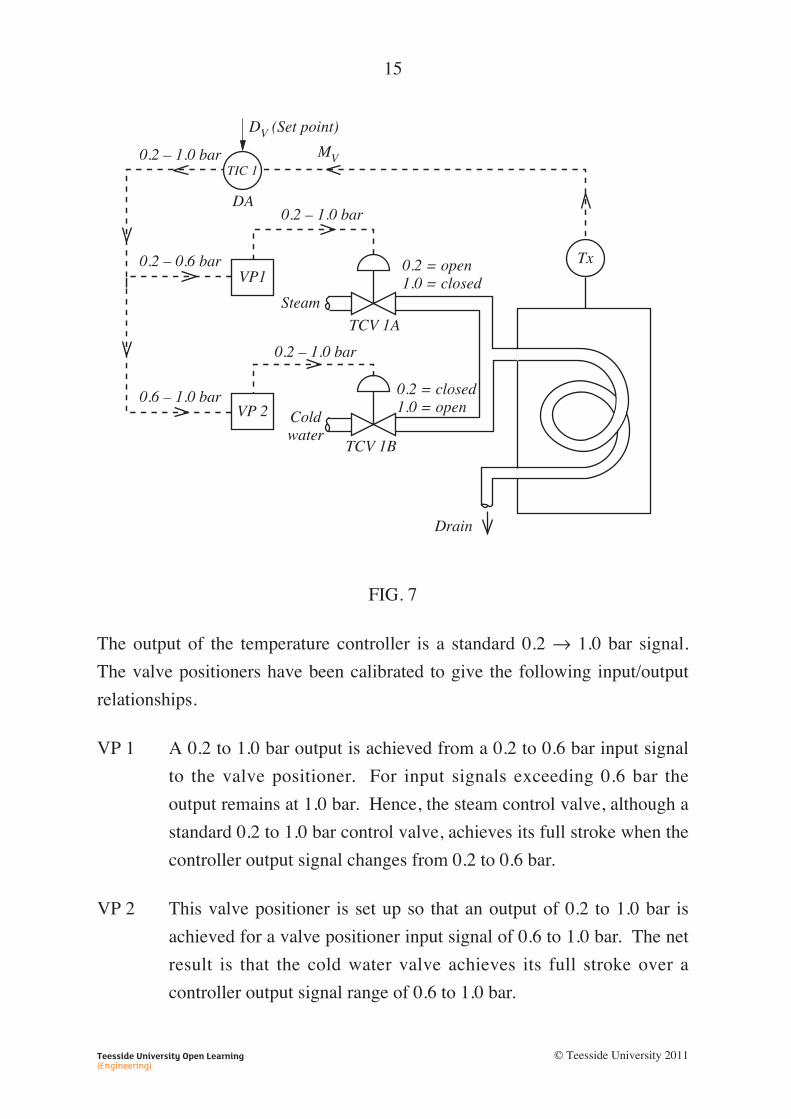
FIG. 7

The output of the temperature controller is a standard 0.2 → 1.0 bar signal.

The valve positioners have been calibrated to give the following input/output

relationships.

VP 1 A 0.2 to 1.0 bar output is achieved from a 0.2 to 0.6 bar input signal

to the valve positioner. For input signals exceeding 0.6 bar the

output remains at 1.0 bar. Hence, the steam control valve, although a

standard 0.2 to 1.0 bar control valve, achieves its full stroke when the

controller output signal changes from 0.2 to 0.6 bar.

VP 2 This valve positioner is set up so that an output of 0.2 to 1.0 bar is

achieved for a valve positioner input signal of 0.6 to 1.0 bar. The net

result is that the cold water valve achieves its full stroke over a

controller output signal range of 0.6 to 1.0 bar.

Tx

Drain

DV (Set point)

MV0.2 – 1.0 bar

0.2 – 1.0 bar

0.2 – 0.6 bar

0.6 – 1.0 bar

0.2 – 1.0 bar

0.2 = open1.0 = closed

0.2 = closed1.0 = open

VP1

VP 2

Steam

Coldwater

TCV 1A

TCV 1B

DA

TIC 1

15



The system operates in the following manner.

• If the measured value of the process temperature is exactly at the

desired value, the controller output will be 0.6 bar, which represents a

50% bias output. This means that the output of VP 1 will be 1.0 bar

and the steam valve will be closed. The output of VP 2 will be

0.2 bar which means that the cold water valve will also be closed.

These valve states are correct for the stated conditions because there

is no heating or cooling requirement.

• If the process temperature rises above the desired value, the

controller output will exceed 0.6 bar. This will not affect the position

of the steam valve, but positioner VP2 will respond to give an

increased output and open the cold water valve. This action will, of

course, reduce the process fluid temperature.

• If the process temperature drops below the desired value the

controller output will fall below 0.6 bar. The water valve will remain

closed but VP 1 will come into operation to open the steam valve and

raise the process fluid temperature.

Note that when split range valves are employed, only one valve is in operation

at any particular time. The obvious exception to this occurs when the

controller output is 0.6 bar, putting both control valves into the closed position.

16



Advantages of using a Valve Positioner

• An increased pressure is supplied to the valve actuator, thereby

ensuring the following outcomes:

(a) the valve always reaches its correct position corresponding to

the applied input signal

(b) compensation for the effect of valve stem friction is achieved

(c) any high process line pressures affecting the actuator are

overcome.

• The use of a cam permits variation of the control signal/flow

characteristic relationship.

• Faster positioning with less overshoot is achieved.

• Split range control valves can be used.

• Control valves of different operating ranges can be used.

• Reverse or direct valve action can be employed in order to change

the "apparent action" of a valve while retaining the original air failure

action.

17



________________________________________________________________________________________

CONTROL VALVE SIZING________________________________________________________________________________________

We now need to consider how the size of a control valve is determined.

It is extremely important to select a valve of the correct size. A valve which is

too small to deliver the required flow will probably need to be replaced at a

later date. A valve which is too large for its application incurs unnecessary

expense and will provide inferior control.

Despite careful selection of the correct controller and correct calibration of the

instrument system, effective process control will be difficult to achieve using

incorrectly sized valves.

The correct sizing of a control valve should ensure the selection of a valve

capable of passing a desired maximum flow. The flow through a control valve,

which can be regarded as a restriction, is given by the expression:

Representing all other constants by the single constant C, the relationship can

be expressed in the following form:

Q Cp= ∆

ρ

where, flow ratedifferential pres

Qp

==∆ ssure across the restriction

fluid densityρ =AAA

1

2

==

area of pipearea of restriction.

QA A

A A

p=( )

×1 2

1 2

2

–

∆ρ

18



The value of C can be determined experimentally. Normally, the constant C is

represented by Cv which is termed the valve flow coefficient. Hence, the

expression becomes:

British Standards (Industrial-process control valves BS EN 60534-2-1) defines

a valve’s flow coefficient for when the liquid is water as:

The volume flow of water through a valve measured in cubic metres per

hour with a pressure drop of 1 bar across the valve and at a water

temperature in the range of 5ºC to 40° C.

As the liquid is water and the temperature range is small we can assume that

density (ρ) is constant and we can incorporate it into the constant. We can thus

use the above definition to define a new valve flow coefficient for water (Kv)

as:

where: is the volumetric flow througQ hh the valve in cubic metres per hour is∆p the measured differential pressure drop accross the valve in bar

is the pressure v

∆pK lloss of 1 bar.

K Qp

pK

vv=

∆

∆

Q Cp

C Qp

=

=

v

vor

∆

∆

ρ

ρ

19



Determine the units of KV.

...................................................................................................................................................

...................................................................................................................................................

...................................................................................................................................................

...................................................................................................................................................

...................................................................................................................................................

________________________________________________________________________________________

If a liquid other than water is used to determine the flow coefficient, then the

equation needs to take account of the different densities of the water and the

new liquid, and can be modified to:

where: is the measured differential pr∆p eessure drop across the valve in bar is ρ tthe density of the liquid in kg m is t

–3

wρ hhe density of water in kg m

is the rel

–3

RD aative density of the liquid =

has beew

v

ρρ

∆pK nn replaced by 1 bar.

K Qp

p

K Qp

R

Kv

w

v

v

OR

=⎛

⎝⎜⎞

⎠⎟×

=⎛⎝⎜

⎞⎠⎟

×

∆

∆

∆

ρρ

1DD

Since the term inside the squarevvK Q

p

pK=

∆∆

root is dimensionless, and thus has

thevK

same units as namely m h3 –1Q, .

20



Thus, if we know the value of Kv, then the volumetric flow through a valve can

be found by transforming this equation to make Q the subject, i.e.

Alternative flow coefficient Cv

Kv is the metric value of valve flow coefficient. The United States still uses

flow coefficients based upon the US gallon (0.833 of the imperial gallon) and

pressure measured in pounds per square inch (p.s.i.). Such is the prevalence of

US instrumentation that British Standards actually define an alternative flow

coefficient in ‘US’ units. When defined as such, the flow coefficient is given

the symbol Cv.

The US valve flow coefficient Cv is therefore defined as:

The volume flow in US gallons per minute through the valve with a pressure

drop of 1 p.s.i. across the valve and at a water temperature in the range of

40°F to 100ºF.

Using this definition, Cv is given by:

Cv will have units of US gallons per minute.

where, is the volumetric flow throughQ the valve in US gallons per minute is t∆p hhe measured differential pressure drop acrooss the valve in p.s.i.is the pressure

v∆pC loss of 1 p.s.i.

C Qp

pC

vv=

∆

∆

Q Kp

RD= v

∆

21



(These alternative definitions of flow coefficients reveal why the standard has

had to define the parameters ∆pKvand ∆pCv

so that they have the different

values of 1 bar and 1 p.s.i. respectively.)

Installed Conditions

In a practical industrial application the installed flow performance of a valve

can be greatly affected by:

• the type of valve

• the presence of other fittings such as reducers and trims

• the piping arrangements surrounding the valve.

BS EN 60534-2-1 allows for the modifying effects of valve type, fixtures and

piping in installed conditions by including correction factors in the design

equations. For example, the equations can be modified by using correction

factors Fd and FP (valve design and piping geometry factors respectively). The

application of these factors is quite complex and will not be pursued any

further in this lesson. For more information, refer to the standard.

On another practical point, the differential pressure across a valve varies with

where the two measuring points are made along the pipework. FIGURE 8

shows the BS recommended tapping points on the pipeline at which the

differential pressure measurements should be made. For a pipe of diameter D,

the upstream measurement point should be made at a distance of 2D from the

flange of the valve and the downstream measurement point should be made at

a distance of 6D.

22



FIG. 8

VALVE SIZING FOR LIQUID FLOW

Knowing the value of Kv, we can refer to manufacturers' tables to determine

the valve size required. TABLE 1 shows a typical set of manufacturer’s

empirical data for a particular type of valve, relating valve size to flow

coefficient. Many valve manufacturers also produce charts and web-based

software to aid in valve sizing.

TABLE 1

Valve nominal size (dia) Flow co-efficient

mm

6

10

15

20

25

40

50

60

75

100

inches

1

1

2

2

3

4

KV

0.70

1.45

2.75

5.85

11.1

24.2

41.3

60.1

86.1

142

CV

0.81

1.68

3.19

6.79

12.88

28.07

47.91

69.72

99.88

164.72

14381234

12

12

Valve

2D 6D

D

1 2

Flow

23



We can determine the Kv value of a valve when given the required flow rate Q

(in m3 h–1), the relative density RD of the process liquid and the pressure drop

∆p across the valve in bar.

All of the above equations are valid when:

• the flow is turbulent

• the nominal diameter of the valve is matched to that of the pipe

• cavitation or flashing does not occur.

The equations have to be modified however, if the flow is laminar or if

cavitation or flashing occur.

Example 1

When a valve passes a water flow of 1 litre per second the pressure drop across

it is 0.5 bar. Calculate the Kv of the valve.

Solution

Q

K QRD

p

= =

= =

136001000

36001

litre s m h–1 3 –1

v ∆ 00001

0 5

5 1

.

.Kv =

24



________________________________________________________________________________________

RANGEABILITY AND TURNDOWN RATIO________________________________________________________________________________________

It is impossible for a control valve to maintain control over a process fluid

whilst the valve stem is at an extreme point of its travel. The term

rangeability, as applied to a control valve, is the ratio of the maximum

controllable flow to the minimum controllable flow, and is indicative of the

range over which the inherent characteristics of the valve are maintained.

In most applications, control valves do not normally function at their

maximum rated flow conditions. The normal rated flow is, in practice, about

70% of the maximum rated flow rate. Turndown ratio is the ratio of normal

rated flow rate to the minimum controllable flow rate.

25



________________________________________________________________________________________

PROCESS PROBLEMS________________________________________________________________________________________

Noise

Control valves handling fluids, especially at high flow rates and pressures, are

often subject to 'noise' production. This unwanted 'noise' is produced as a

result of the random pressure fluctuations within the valve body and/or the

impingement of fluid on valve components. It may be loud enough to present

a health hazard, or it may possess a resonant frequency, leading to vibration

within the valve trim and possible early failure of the valve.

Flashing and Cavitation

If the pressure drop across a valve is too great, the downstream pressure of the

fluid might fall below the vapour pressure of the liquid. In such circumstances

some of the liquid will vaporise, producing a phenomenon known as flashing

as illustrated in FIGURE 9.

The fluid passing through the valve becomes a mixture of vapour and liquid.

The vapour is normally in the form of bubbles, which results in two

undesirable effects.

• The calculated flow will be incorrect for the liquid and vapour

mixture.

• Cavitation can result as the downstream pressure rises above the

vapour pressure, causing the bubbles to collapse. The bubbles

normally collapse on the valve trim or body or in the pipe, creating

large localised pressures which cause rapid wear in addition to excess

noise.

26



FIG. 9

OVERCOMING THE PROBLEMS OF NOISE, FLASHING AND CAVITATION

Excessive 'noise' can cause damage to plant, personnel or equipment. Its

effects can be reduced by fitting lagging and pipe silencers similar to those

found on vehicles. These measures deal with most of the damaging

frequencies, and reduce the effects of the noise problem. Care must be

exercised when using pipe silencers as they tend to act as pressure reducers

and fluid flow restrictors.

Cavitation is the end result of flashing caused by high pressure drops across

the valve. Reducing the pressure drop, or increasing the inlet pressure to

prevent the pressure falling below the vapour pressure, removes the risks of

flashing and cavitation occurring. The inlet pressure may be increased by

installing the valve at a lower location in the pipe system. If this is not

Pressure

Maximum peak velocity

Stream velocity

Fluid pressure

CavitationBubblescollapse

Flashing

Bubblesform

Vapourpressure

Distance

Flow

Flashing and Cavitation

27



possible then the use of an anti-cavitation trim as shown in FIGURE 10 is

recommended.

FIG. 10

This type of valve trim reduces the likelihood of flashing, cavitation and noise

in the following ways.

• Division of the flow into several streams induces several smaller

velocity peaks occurring at slightly different times. The maximum

peak velocity is also reduced and, because the line pressure is

maintained above the vapour pressure, flashing is prevented.

• The flow path through the small orifices reduces the potential energy

of the fluid, leaving less energy available for noise conversion.

You should now be able to attempt the following Self-Assessment Questions.

28



________________________________________________________________________________________

NOTES________________________________________________________________________________________

...................................................................................................................................................

...................................................................................................................................................

...................................................................................................................................................

...................................................................................................................................................

...................................................................................................................................................

...................................................................................................................................................

...................................................................................................................................................

...................................................................................................................................................

...................................................................................................................................................

...................................................................................................................................................

...................................................................................................................................................

...................................................................................................................................................

...................................................................................................................................................

...................................................................................................................................................

...................................................................................................................................................

...................................................................................................................................................

...................................................................................................................................................

...................................................................................................................................................

...................................................................................................................................................

...................................................................................................................................................

...................................................................................................................................................

...................................................................................................................................................

...................................................................................................................................................

...................................................................................................................................................

...................................................................................................................................................

...................................................................................................................................................

...................................................................................................................................................

...................................................................................................................................................

...................................................................................................................................................

...................................................................................................................................................

29



________________________________________________________________________________________

SELF-ASSESSMENT QUESTIONS________________________________________________________________________________________

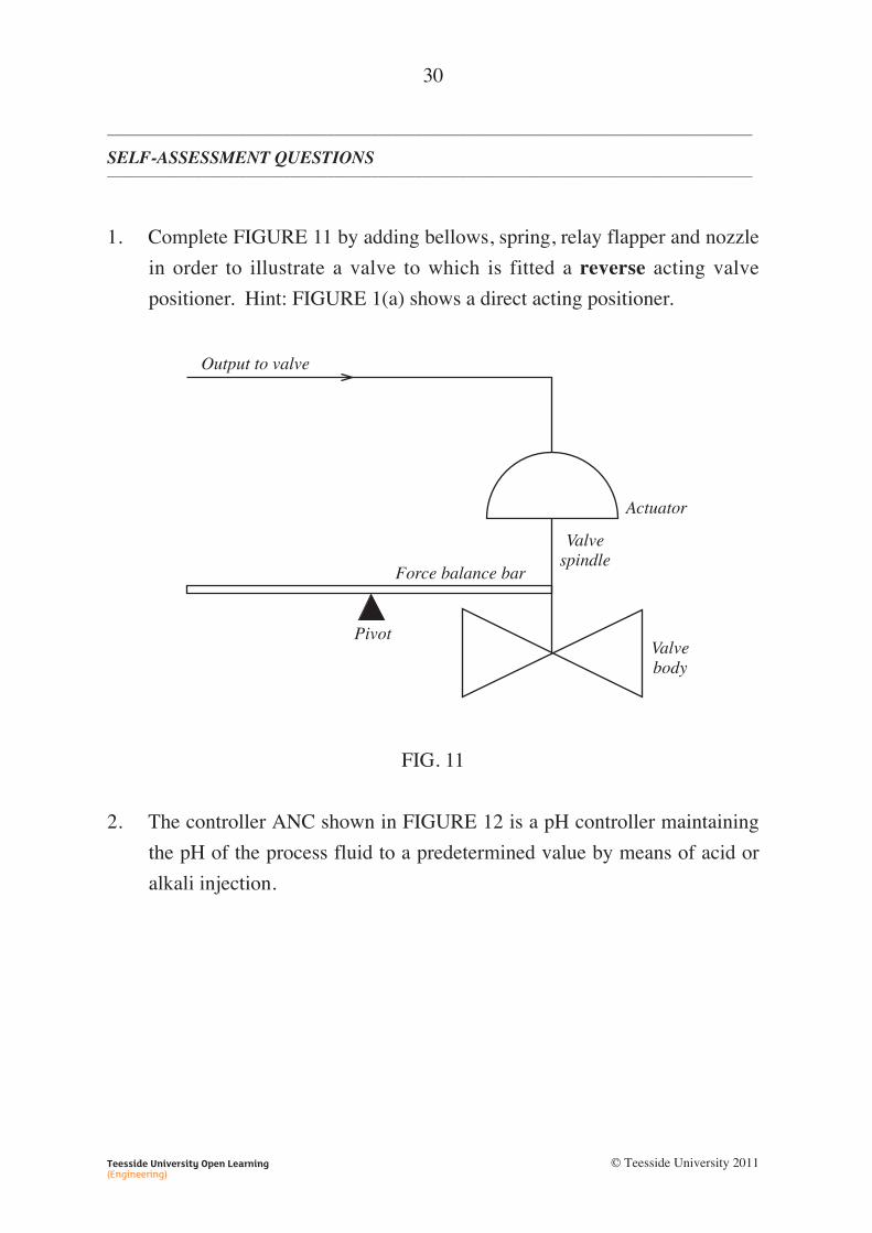
1. Complete FIGURE 11 by adding bellows, spring, relay flapper and nozzle

in order to illustrate a valve to which is fitted a reverse acting valve

positioner. Hint: FIGURE 1(a) shows a direct acting positioner.

FIG. 11

2. The controller ANC shown in FIGURE 12 is a pH controller maintaining

the pH of the process fluid to a predetermined value by means of acid or

alkali injection.

Output to valve

Actuator

Valvespindle

Force balance bar

PivotValvebody

30



FIG. 12

The output of ANC is 0.2 bar when the process fluid is too alkaline and

1.0 bar when too acidic. Valves A and B both work on a standard

0.2 → 1.0 bar signal. Show the piping arrangement and stipulate the

ranges of the valve positioners. Also state the fail safe position for each

valve to ensure the process fluid remains acidic in the event of an

Instrument Air Supply failure.

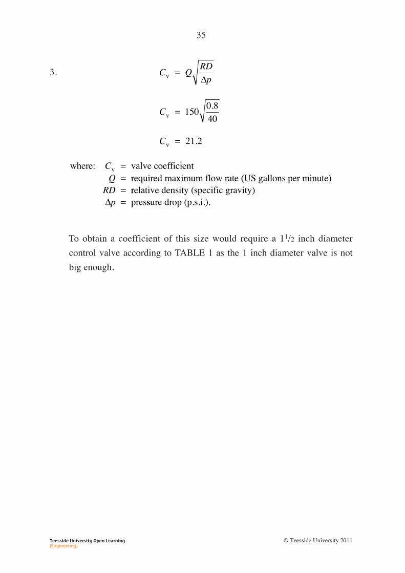
3. Determine the Cv value for a valve required to pass a maximum of

150 US gallons of ethyl alcohol per minute which has a relative density of

0.8, at a maximum pressure drop of 40 psi. Use TABLE 1 in the lesson to

determine the required valve size.

Process flow

ANCV B

ANCV A

Acid injection

Alkali injection

ANC 1

31



________________________________________________________________________________________

ANSWERS TO SELF-ASSESSMENT QUESTIONS________________________________________________________________________________________

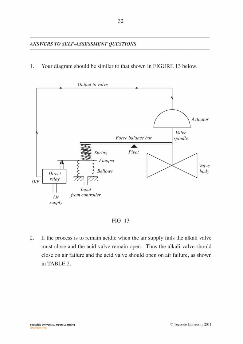
1. Your diagram should be similar to that shown in FIGURE 13 below.

FIG. 13

2. If the process is to remain acidic when the air supply fails the alkali valve

must close and the acid valve remain open. Thus the alkali valve should

close on air failure and the acid valve should open on air failure, as shown

in TABLE 2.

Output to valve

Force balance bar

Pivot

Actuator

Valvespindle

Valvebody

Spring

Flapper

Bellows

Inputfrom controller

O/P

Airsupply

Directrelay

32



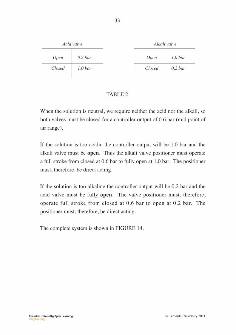
TABLE 2

When the solution is neutral, we require neither the acid nor the alkali, so

both valves must be closed for a controller output of 0.6 bar (mid point of

air range).

If the solution is too acidic the controller output will be 1.0 bar and the

alkali valve must be open. Thus the alkali valve positioner must operate

a full stroke from closed at 0.6 bar to fully open at 1.0 bar. The positioner

must, therefore, be direct acting.

If the solution is too alkaline the controller output will be 0.2 bar and the

acid valve must be fully open. The valve positioner must, therefore,

operate full stroke from closed at 0.6 bar to open at 0.2 bar. The

positioner must, therefore, be direct acting.

The complete system is shown in FIGURE 14.

Alkali valve

Open

Closed

1.0 bar

0.2 bar

Acid valve

Open

Closed

0.2 bar

1.0 bar

33



FIG. 14

O.A.F.

C.A.F.

VPDirectacting

VPDirectacting0.6 bar

1.0 bar

0.2 bar0.6 bar

Output

0.2 baropen Air to

close

Air toopenOpen

1.0 bar

Process flow

ANCV B

ANCV A

Acid injection

Alkali injection

ANC 1

1.0 barclosed

Closed0.2 bar

0.2 Too alkali0.6 Neutral1.0 Too acid

34



3.

To obtain a coefficient of this size would require a 11/2 inch diameter

control valve according to TABLE 1 as the 1 inch diameter valve is not

big enough.

where: valve coefficientrequired ma

vCQ

== xximum flow rate (US gallons per minute)

RD = rrelative density (specific gravity)pres∆p = ssure drop (p.s.i.).

C QRD

p

C

C

v

v

v

=

=

=

∆

1500 840

21 2

.

.

35



________________________________________________________________________________________

SUMMARY________________________________________________________________________________________

A valve positioner ensures that the valve stem is positioned accurately and

rapidly.

Valve positioners can be either reverse or direct acting.

The gain of a valve positioner can be adjusted to achieve split range operation.

Split range operation occurs when different ranges of the output from a

controller control different valves via individual valve positioners. The valve

positioners are calibrated so that they are actuated by different sub-ranges of

the controller signal.

The spring location in a control valve determines the position the valve stem

assumes in the event of an air failure occurring. In conjunction with the

arrangement of the valve trim, it determines whether the valve is Open Air

Failure (OAF) or Close Air Failure (CAF).

The flow coefficient Cv is used in control valve sizing. By definition, the Cv

has a value equal to 1.0 when a fully open valve will pass a flow rate of 1

US gall min–1 of water when a pressure drop of 1 psi occurs across the valve.

The metric equivalent is Kv (1 m3 h–1 when pressure drop is 1 bar).

Rapid flow of fluids through valves can cause problems due to noise and

vibration. When large pressure drops occur across valves in liquid flow

applications it is possible for "flashing" to occur. 'Flashing' occurs when a

rapid reduction in pressure allows vapour bubbles to form within the liquid.

When these bubbles collapse due to the extremely high local pressures that can

be created, 'cavitation', which can lead to rapid erosion of valve internals, can

result. The correct selection of valve trim can reduce the likelihood of these

problems occurring.

36



Documents

MODULE TITLE : CONTROL SYSTEMS AND AUTOMATION TOPIC … · LESSON 2 : VALVE POSITIONERS AND VALVE SIZING CSA - 4 - 2 ... the pivot point of the force balance bar. This allows the