MODULE I. SAMPLING METHODOLOGY

2

Chapter 1. GENERAL INTRODUCTION Decision makers make better decisions when they use all available information in an effective and meaningful way. The primary role of statistics is to provide decision makers with methods for obtaining and analyzing information to help make these decisions. Statistics is used to answer long-range planning questions, such as when and where to locate facilities to handle future sales. Definition Statistics is defined as the science of collecting, organizing, presenting, analyzing and interpreting numerical data for the purpose of assisting in making a more effective decision. Types of Statistics There are two types of statistics. 1. Descriptive Statistics is concerned with summary calculations, graphs, charts and tables. 2. Inferential Statistics is a method used to generalize from a sample to a population. For example, the average income of all families (the population) in the US can be estimated from figures obtained from a few hundred (the sample) families. Statistical Population Is the collection of all possible observations of a specified characteristic of interest. An example is all of the REMA staff. Note that a sample is a subset of the population. Variable A variable is an item of interest that can take on many different numerical values. Types of Variables or Data 1. Qualitative Variables are nonnumeric variables and can't be measured. Examples include gender, religious affiliation, state of birth. 2. Quantitative Variables are numerical variables and can be measured. Examples include balance in your checking account, number of children in your family. Note that quantitative variables are either discrete (which can assume only certain values, and there are usually "gaps" between the values, such as the number of bedrooms in your house) or continuous (which can assume any value within a specific range, such as the air pressure in a tire.) Types of Quantitative Data: There are four (4) types of quantitative data: 1. Nominal Data: The weakest data measurement. Numbers are used to represent an item or characteristic. Example: designating male=1 and female=2

3

2. Ordinal or Rank Data: Numbers are used to rank. Example is excellent, good, fair and poor. The main difference between ordinal data and nominal data is that ordinal data contain both an equality (=) and a greater-than (>) relationship, whereas the nominal data contain only an equality (=) relationship. 3. Interval Data: If we have data with ordinal properties (> & =) and can also measure the distance between two data items, we have an interval measurement. Interval data are preferred over ordinal data because, with them, decision makers can precisely determine the difference between two observations, i.e., distances between numbers can be measured. For example, frozen-food packagers have daily contact with a common interval measurement--temperature. 4. Ratio Data: Is the highest level of measurement and allows for all basic arithmetic operations, including division and multiplication. Data measured on a ratio scale have a fixed or no arbitrary zero point. Examples include business data, such as cost, revenue and profit. Sources of Data: 1. Secondary Data: Data which are already available. An example: statistical abstract of USA. Advantage: less expensive. Disadvantage: may not satisfy your needs. 2. Primary Data: Data which must be collected. Methods of Collecting Primary Data: 1. Focus Group; 2. Telephone Interview; 3. Mail Questionnaires; 4. Door-to-Door Survey; 5. Mall Intercept; 6. New Product Registration; 7. Personal Interview; and 8. Experiments are some of the sources for collecting the primary data. 1.1 Sampling Methods There are many ways to collect a sample. The most commonly used methods are: A. Statistical Sampling: 1. Simple Random Sampling: Is a method of selecting items from a population such that every possible sample of specific size has an equal chance of being selected. In this case, sampling may be with or without replacement. 2. Stratified Random Sampling: Is obtained by selecting simple random samples from strata (or mutually exclusive sets). Some of the criteria for dividing a population into strata are: Sex (male, female); Age (under 18, 18 to 28, 29 to 39); Occupation (blue-collar, professional, other). 3. Cluster Sampling: Is a simple random sample of groups or cluster of elements. Cluster sampling is useful when it is difficult or costly to generate a simple random sample. For example, to estimate the average annual household income in a large city we use cluster sampling, because to use simple random sampling we need a complete list of households in the city from which to sample. To use stratified random sampling, we would again need the list of households. A less expensive way is to let each block within the city represent a cluster.

4

A sample of clusters could then be randomly selected, and every household within these clusters could be interviewed to find the average annual household income. B. Nonstatistical Sampling: 1. Judgment Sampling: In this case, the person taking the sample has direct or indirect control over which items are selected for the sample. 2. Convenience Sampling: In this method, the decision maker selects a sample from the population in a manner that is relatively easy and convenient. 3. Quota Sampling: In this method, the decision maker requires the sample to contain a certain number of items with a given characteristic. Many political polls are, in part, quota sampling. SAMPLING Sampling is that part of statistical practice concerned with the selection of a subset of individual observations within a population of individuals intended to yield some knowledge about the population of concern, especially for the purposes of making predictions based on statistical inference. Sampling is an important aspect of data collection. Researchers rarely survey the entire population for two reasons: the cost is too high, and the population is dynamic in that the individuals making up the population may change over time. The three main advantages of sampling are that the cost is lower, data collection is faster, and since the data set is smaller it is possible to ensure homogeneity and to improve the accuracy and quality of the data. Each observation measures one or more properties (such as weight, location, color) of observable bodies distinguished as independent objects or individuals. In survey sampling, survey weights can be applied to the data to adjust for the sample design. Results from probability theory and statistical theory are employed to guide practice. In business and medical research, sampling is widely used for gathering information about a population. SAMPLING PROCESS The sampling process comprises several stages: 1. Defining the population of concern 2. Specifying a sampling frame, a set of items or events possible to measure 3. Specifying a sampling method for selecting items or events from the frame 4. Determining the sample size 5. Implementing the sampling plan 6. Sampling and data collecting POPULATION DEFINITION Successful statistical practice is based on focused problem definition. In sampling, this includes defining the population from which our sample is drawn. A population can be defined as including all people or items with the characteristic one wishes to understand. Because there is very rarely enough time or money to gather information from everyone or

5

everything in a population, the goal becomes finding a representative sample (or subset) of that population. Sometimes that which defines a population is obvious. For example, a manufacturer needs to decide whether a batch of material from production is of high enough quality to be released to the customer, or should be sentenced for scrap or rework due to poor quality. In this case, the batch is the population. Although the population of interest often consists of physical objects, sometimes we need to sample over time, space, or some combination of these dimensions. For instance, an investigation of supermarket staffing could examine checkout line length at various times, or a study on endangered penguins might aim to understand their usage of various hunting grounds over time. For the time dimension, the focus may be on periods or discrete occasions. SAMPLING FRAME In the most straightforward case, such as the sentencing of a batch of material from production (acceptance sampling by lots), it is possible to identify and measure every single item in the population and to include any one of them in our sample. However, in the more general case this is not possible. There is no way to identify all rats in the set of all rats. Where voting is not compulsory, there is no way to identify which people will actually vote at a forthcoming election (in advance of the election). These imprecise populations are not amenable to sampling in any of the ways below and to which we could apply statistical theory. As a remedy, we seek a sampling frame which has the property that we can identify every single element and include any in our sample. The most straightforward type of frame is a list of elements of the population (preferably the entire population) with appropriate contact information. For example, in an opinion poll, possible sampling frames include: • Electoral register • Telephone directory Not all frames explicitly list population elements. For example, a street map can be used as a frame for a door-to-door survey; although it doesn't show individual houses, we can select streets from the map and then visit all houses on those streets. (One advantage of such a frame is that it would include people who have recently moved and are not yet on the list frames discussed above.) The sampling frame must be representative of the population and this is a question outside the scope of statistical theory demanding the judgment of experts in the particular subject matter being studied. All the above frames omit some people who will vote at the next election and contain some people who will not; some frames will contain multiple records for the same person. People not in the frame have no prospect of being sampled. Statistical theory tells us about the uncertainties in extrapolating from a sample to the frame. In extrapolating from frame to population, its role is motivational and suggestive. To the scientist, however, representative sampling is the only justified procedure for choosing individual objects for use as the basis of generalization, and is therefore usually the only acceptable basis for ascertaining truth.

6

BASIC PROBLEM OF SAMPLING FRAMES: Missing elements: Some members of the population are not included in the frame. Foreign elements: The non-members of the population are included in the frame. Duplicate entries: A member of the population is surveyed more than once. Groups or clusters: The frame lists clusters instead of individuals.

A frame may also provide additional 'auxiliary information' about its elements; when this information is related to variables or groups of interest, it may be used to improve survey design. For instance, an electoral register might include name and sex; this information can be used to ensure that a sample taken from that frame covers all demographic categories of interest. (Sometimes the auxiliary information is less explicit; for instance, a telephone number may provide some information about location.) Having established the frame, there are a number of ways for organizing it to improve efficiency and effectiveness. It's at this stage that the researcher should decide whether the sample is in fact to be the whole population and would therefore be a census. PROBABILITY AND NON PROBABILITY SAMPLING A probability sampling scheme is one in which every unit in the population has a chance (greater than zero) of being selected in the sample, and this probability can be accurately determined. The combination of these traits makes it possible to produce unbiased estimates of population totals, by weighting sampled units according to their probability of selection. Example: We want to estimate the total income of adults living in a given street. We visit each household in that street, identify all adults living there, and randomly select one adult from each household. (For example, we can allocate each person a random number, generated from a uniform distribution between 0 and 1, and select the person with the highest number in each household). We then interview the selected person and find their income. People living on their own are certain to be selected, so we simply add their income to our estimate of the total. But a person living in a household of two adults has only a one-in-two chance of selection. To reflect this, when we come to such a household, we would count the selected person's income twice towards the total. (In effect, the person who is selected from that household is taken as representing the person who isn't selected.) In the above example, not everybody has the same probability of selection; what makes it a probability sample is the fact that each person's probability is known. When every element in the population does have the same probability of selection, this is known as an 'equal probability of selection' (EPS) design. Such designs are also referred to as 'self-weighting' because all sampled units are given the same weight. PROBABILITY SAMPLING Probability sampling includes: Simple Random Sampling, Systematic Sampling, Stratified Sampling, Probability Proportional to Size Sampling, and Cluster or Multistage Sampling. These various ways of probability sampling have two things in common: • Every element has a known nonzero probability of being sampled and • Involves random selection at some point.

7

NON PROBABILITY SAMPLING Nonprobability sampling is any sampling method where some elements of the population have no chance of selection (these are sometimes referred to as 'out of coverage'/'undercovered'), or where the probability of selection can't be accurately determined. It involves the selection of elements based on assumptions regarding the population of interest, which forms the criteria for selection. Hence, because the selection of elements is nonrandom, nonprobability sampling does not allow the estimation of sampling errors. These conditions give rise to exclusion bias, placing limits on how much information a sample can provide about the population. Information about the relationship between sample and population is limited, making it difficult to extrapolate from the sample to the population. Example: We visit every household in a given street, and interview the first person to answer the door. In any household with more than one occupant, this is a nonprobability sample, because some people are more likely to answer the door (e.g. an unemployed person who spends most of their time at home is more likely to answer than an employed housemate who might be at work when the interviewer calls) and it's not practical to calculate these probabilities. Nonprobability Sampling includes: Quota Sampling and Purposive Sampling. In addition, nonresponse effects may turn any probability design into a nonprobability design if the characteristics of nonresponse are not well understood, since nonresponse effectively modifies each element's probability of being sampled. SAMPLING METHODS Within any of the types of frame identified above, a variety of sampling methods can be employed, individually or in combination. Factors commonly influencing the choice between these designs include: • Nature and quality of the frame • Availability of auxiliary information about units on the frame • Accuracy requirements, and the need to measure accuracy • Whether detailed analysis of the sample is expected • Cost/operational concerns

8

Chapter 2. SIMPLE RANDOM SAMPLING In a simple random sample ('SRS') of a given size, all such subsets of the frame are given an equal probability. Each element of the frame thus has an equal probability of selection: the frame is not subdivided or partitioned. Furthermore, any given pair of elements has the same chance of selection as any other such pair (and similarly for triples, and so on). This minimizes bias and simplifies analysis of results. In particular, the variance between individual results within the sample is a good indicator of variance in the overall population, which makes it relatively easy to estimate the accuracy of results. However, SRS can be vulnerable to sampling error because the randomness of the selection may result in a sample that doesn't reflect the makeup of the population. For instance, a simple random sample of ten people from a given country will on average produce five men and five women, but any given trial is likely to over represent one sex and under represent the other. Systematic and stratified techniques, discussed below, attempt to overcome this problem by using information about the population to choose a more representative sample. SRS may also be cumbersome and tedious when sampling from an unusually large target population. In some cases, investigators are interested in research questions specific to subgroups of the population. For example, researchers might be interested in examining whether cognitive ability as a predictor of job performance is equally applicable across racial groups. SRS cannot accommodate the needs of researchers in this situation because it does not provide subsamples of the population. Stratified sampling, which is discussed below, addresses this weakness of SRS. II.1. Sampling distribution The sampling distribution of a statistic is a fundamental concept of statistical inference. In this chapter we will focus on the average sample and sampling distribution. We first present some definitions of terms and important relations in determining the sampling distribution.

• Expected Value The expected value is the average value of a feature from all possible samples of the same size. Mathematically, we define the expected value or average of a random variable Y as follows:

∑=y

ypyyE )(.)( where 1)( =∑y

yp

The expected value is the sum of products of all possible values of variable Y and their associated probabilities p(y). For example, consider the following table data from a census where the variable Y is the size of a randomly selected household:

Size Number of Households

Percentage

1 Person 2 persons 3 persons 4 persons

17 816 24 734 13 845 12 470

0,225 0,313 0,175 0,157

9

5 persons 6 persons 7 persons or more

5 996 2 499 1 748

0,076 0,032 0,022

Total 79 108 1,00 E(y) = 1. (0,225) + 2. (0,313) + 3. (0,175) + 4. (0,157) + 5. (0,076) + 6. (0,032) + 7,7. (0,022) = 2,75 This means that the average of these different sizes of household is 2.75. Note that the size of household "7 or more" is the aggregation of data for households where Y = 7, 8, 9 ... We determined the average size of all households with 7 or more persons, or 7.7.

• Unbiased estimator An estimator is unbiased when its expected value is equal to the parameter that it is advantageous to estimate. Thus, the bias is the difference between the expected value of an estimate and the true population-value (or parameter) is zero.

• Consisting Estimator

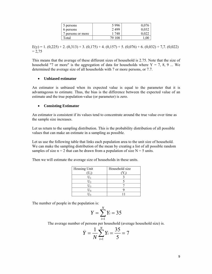
An estimator is consistent if its values tend to concentrate around the true value over time as the sample size increases. Let us return to the sampling distribution. This is the probability distribution of all possible values that can make an estimate in a sampling as possible. Let us use the following table that links each population area to the unit size of household. We can make the sampling distribution of the mean by creating a list of all possible random samples of size n = 2 that can be drawn from a population of size N = 5 units. Then we will estimate the average size of households in these units.

Housing Unit (Ui)

Household size (Yi)

U1 3 U2 5 U3 7 U4 9 U5 11

The number of people in the population is:

351

== ∑=

N

i

iYY

The average number of persons per household (average household size) is.

75

3511

_=== ∑

=

N

iiY

NY

10

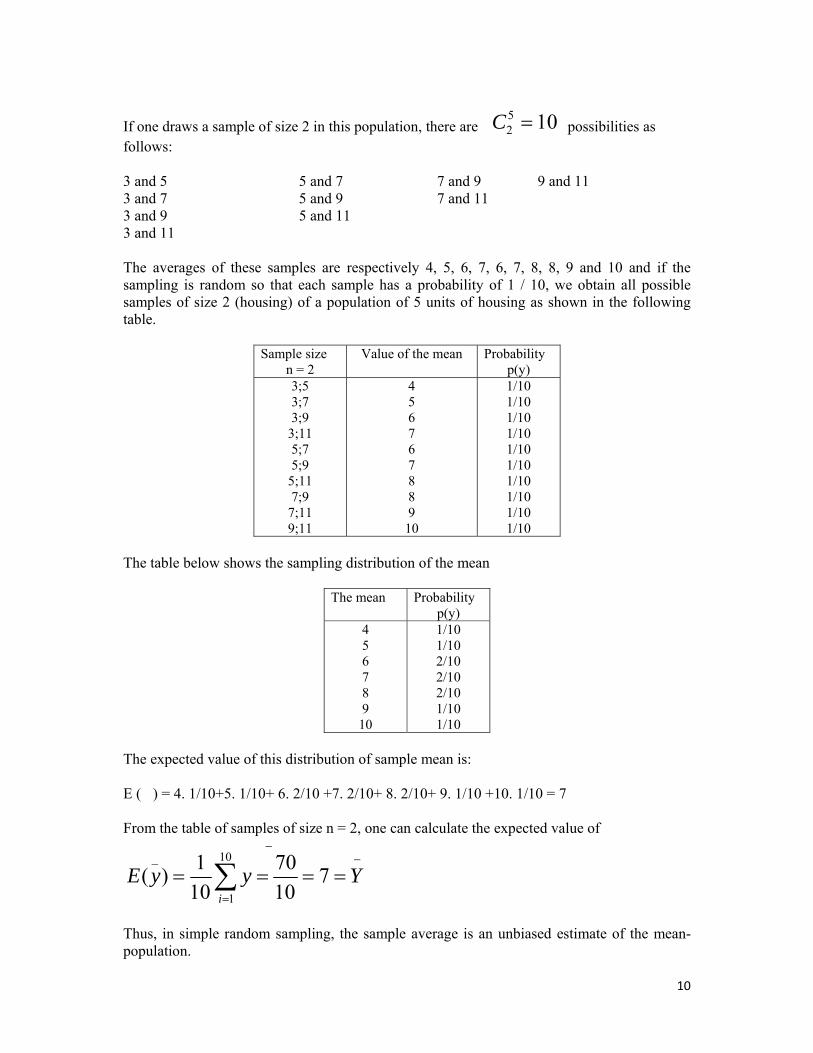
If one draws a sample of size 2 in this population, there are 1052 =C possibilities as

follows: 3 and 5 5 and 7 7 and 9 9 and 11 3 and 7 5 and 9 7 and 11 3 and 9 5 and 11 3 and 11 The averages of these samples are respectively 4, 5, 6, 7, 6, 7, 8, 8, 9 and 10 and if the sampling is random so that each sample has a probability of 1 / 10, we obtain all possible samples of size 2 (housing) of a population of 5 units of housing as shown in the following table.

Sample size n = 2

Value of the mean

Probability p(y)

3;5 3;7 3;9

3;11 5;7 5;9

5;11 7;9

7;11 9;11

4 5 6 7 6 7 8 8 9 10

1/10 1/10 1/10 1/10 1/10 1/10 1/10 1/10 1/10 1/10

The table below shows the sampling distribution of the mean

The mean

Probability p(y)

4 5 6 7 8 9 10

1/10 1/10 2/10 2/10 2/10 1/10 1/10

The expected value of this distribution of sample mean is: E () = 4. 1/10+5. 1/10+ 6. 2/10 +7. 2/10+ 8. 2/10+ 9. 1/10 +10. 1/10 = 7 From the table of samples of size n = 2, one can calculate the expected value of

−

=

−

==== ∑ YyyEi

71070

101)(

10

1

_

Thus, in simple random sampling, the sample average is an unbiased estimate of the mean-population.

11

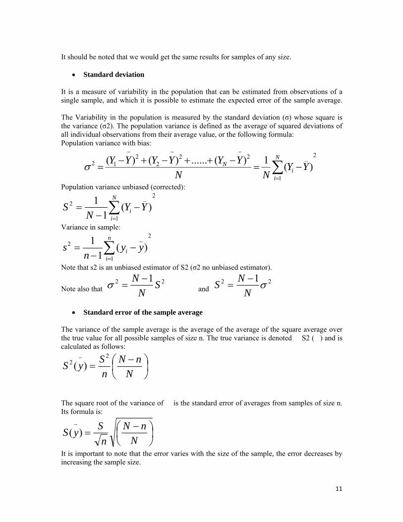
It should be noted that we would get the same results for samples of any size.

• Standard deviation It is a measure of variability in the population that can be estimated from observations of a single sample, and which it is possible to estimate the expected error of the sample average. The Variability in the population is measured by the standard deviation (σ) whose square is the variance (σ2). The population variance is defined as the average of squared deviations of all individual observations from their average value, or the following formula: Population variance with bias:

2

1

_222

212 )(1)(......)()( ∑

=

−−−

−=−++−+−

=N

ii

N YYNN

YYYYYYσ

Population variance unbiased (corrected): 2

1

_2 )(

11 ∑

=

−−

=N

ii YY

NS

Variance in sample: 2

1

_2 )(

11 ∑

=

−−

=n

ii yy

ns

Note that s2 is an unbiased estimator of S2 (σ2 no unbiased estimator).

Note also that 22 1 S

NN −

=σ and 22 1σ

NNS −

=

• Standard error of the sample average

The variance of the sample average is the average of the average of the square average over the true value for all possible samples of size n. The true variance is denoted S2 () and is calculated as follows:

⎟⎠⎞

⎜⎝⎛ −

=−

NnN

nSyS

22 )(

The square root of the variance of is the standard error of averages from samples of size n. Its formula is:

⎟⎠⎞

⎜⎝⎛ −

=−

NnN

nSyS )(

It is important to note that the error varies with the size of the sample, the error decreases by increasing the sample size.

12

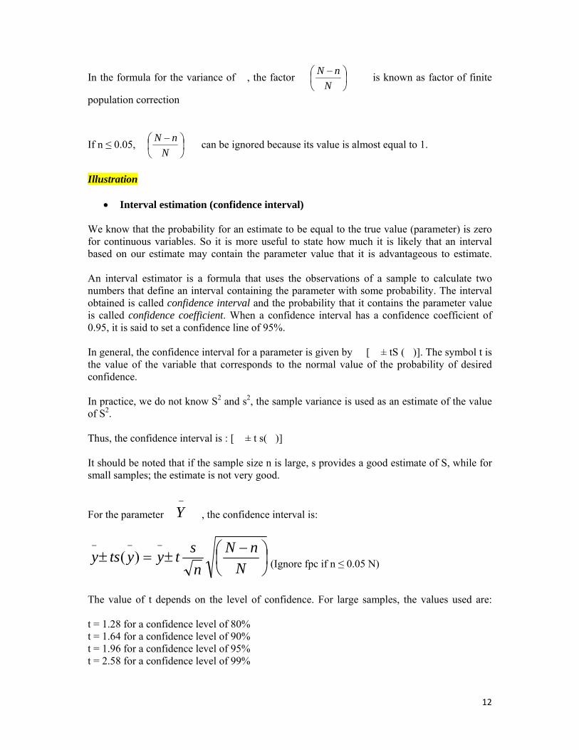
In the formula for the variance of , the factor ⎟⎠⎞

⎜⎝⎛ −

NnN is known as factor of finite

population correction

If n ≤ 0.05, ⎟⎠⎞

⎜⎝⎛ −

NnN can be ignored because its value is almost equal to 1.

Illustration

• Interval estimation (confidence interval) We know that the probability for an estimate to be equal to the true value (parameter) is zero for continuous variables. So it is more useful to state how much it is likely that an interval based on our estimate may contain the parameter value that it is advantageous to estimate. An interval estimator is a formula that uses the observations of a sample to calculate two numbers that define an interval containing the parameter with some probability. The interval obtained is called confidence interval and the probability that it contains the parameter value is called confidence coefficient. When a confidence interval has a confidence coefficient of 0.95, it is said to set a confidence line of 95%. In general, the confidence interval for a parameter is given by [ ± tS ()]. The symbol t is the value of the variable that corresponds to the normal value of the probability of desired confidence. In practice, we do not know S2 and s2, the sample variance is used as an estimate of the value of S2. Thus, the confidence interval is : [ ± t s()] It should be noted that if the sample size n is large, s provides a good estimate of S, while for small samples; the estimate is not very good.

For the parameter −

Y , the confidence interval is:

⎟⎠⎞

⎜⎝⎛ −

±=±−−−

NnN

nstyytsy )( (Ignore fpc if n ≤ 0.05 N)

The value of t depends on the level of confidence. For large samples, the values used are: t = 1.28 for a confidence level of 80% t = 1.64 for a confidence level of 90% t = 1.96 for a confidence level of 95% t = 2.58 for a confidence level of 99%

13

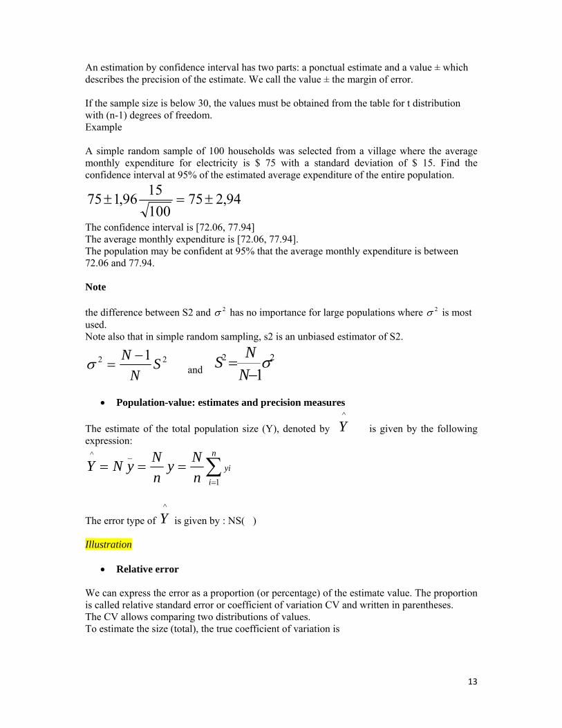
An estimation by confidence interval has two parts: a ponctual estimate and a value ± which describes the precision of the estimate. We call the value ± the margin of error. If the sample size is below 30, the values must be obtained from the table for t distribution with (n-1) degrees of freedom. Example A simple random sample of 100 households was selected from a village where the average monthly expenditure for electricity is $ 75 with a standard deviation of $ 15. Find the confidence interval at 95% of the estimated average expenditure of the entire population.

94,2751001596,175 ±=±

The confidence interval is [72.06, 77.94] The average monthly expenditure is [72.06, 77.94]. The population may be confident at 95% that the average monthly expenditure is between 72.06 and 77.94. Note the difference between S2 and 2σ has no importance for large populations where 2σ is most used. Note also that in simple random sampling, s2 is an unbiased estimator of S2.

22 1 SN

N −=σ and

22

1σ

−=

NNS

• Population-value: estimates and precision measures

The estimate of the total population size (Y), denoted by ^Y is given by the following

expression:

∑=

===n

iyi

nNy

nNyNY

1

_^

The error type of ^Y is given by : NS()

Illustration

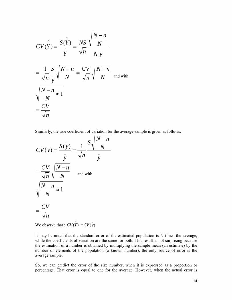
• Relative error We can express the error as a proportion (or percentage) of the estimate value. The proportion is called relative standard error or coefficient of variation CV and written in parentheses. The CV allows comparing two distributions of values. To estimate the size (total), the true coefficient of variation is

14

_^

^^ )()(

yN

NnN

nNS

Y

YSYCV

−

==

NnN

nCV

NnN

y

Sn

−=

−= _

1 and with

1≈−N

nN

nCV

=

Similarly, the true coefficient of variation for the average-sample is given as follows:

__

__ 1)()(

y

NnNS

ny

ySyCV

−

==

NnN

nCV −

= and with

1≈−N

nN

nCV

=

We observe that : )(^YCV = )(

_

yCV It may be noted that the standard error of the estimated population is N times the average, while the coefficients of variation are the same for both. This result is not surprising because the estimation of a number is obtained by multiplying the sample mean (an estimate) by the number of elements of the population (a known number), the only source of error is the average sample. So, we can predict the error of the size number, when it is expressed as a proportion or percentage. That error is equal to one for the average. However, when the actual error is

15

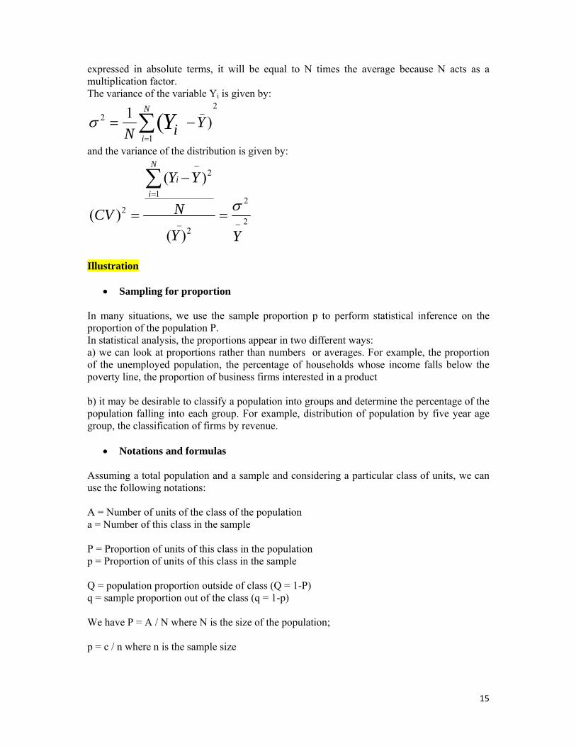
expressed in absolute terms, it will be equal to N times the average because N acts as a multiplication factor. The variance of the variable Yi is given by:

2

1

_2 )1 (∑

=

−=N

iYiN Yσ

and the variance of the distribution is given by:

2

2

_2

2

1

2

)(

)(

)(−

−

=

=

−

=

∑

YY

N

YY

CV

N

ii

σ

Illustration

• Sampling for proportion In many situations, we use the sample proportion p to perform statistical inference on the proportion of the population P. In statistical analysis, the proportions appear in two different ways: a) we can look at proportions rather than numbers or averages. For example, the proportion of the unemployed population, the percentage of households whose income falls below the poverty line, the proportion of business firms interested in a product b) it may be desirable to classify a population into groups and determine the percentage of the population falling into each group. For example, distribution of population by five year age group, the classification of firms by revenue.

• Notations and formulas Assuming a total population and a sample and considering a particular class of units, we can use the following notations: A = Number of units of the class of the population a = Number of this class in the sample P = Proportion of units of this class in the population p = Proportion of units of this class in the sample Q = population proportion outside of class (Q = 1-P) q = sample proportion out of the class (q = 1-p) We have P = A / N where N is the size of the population; p = c / n where n is the sample size

16

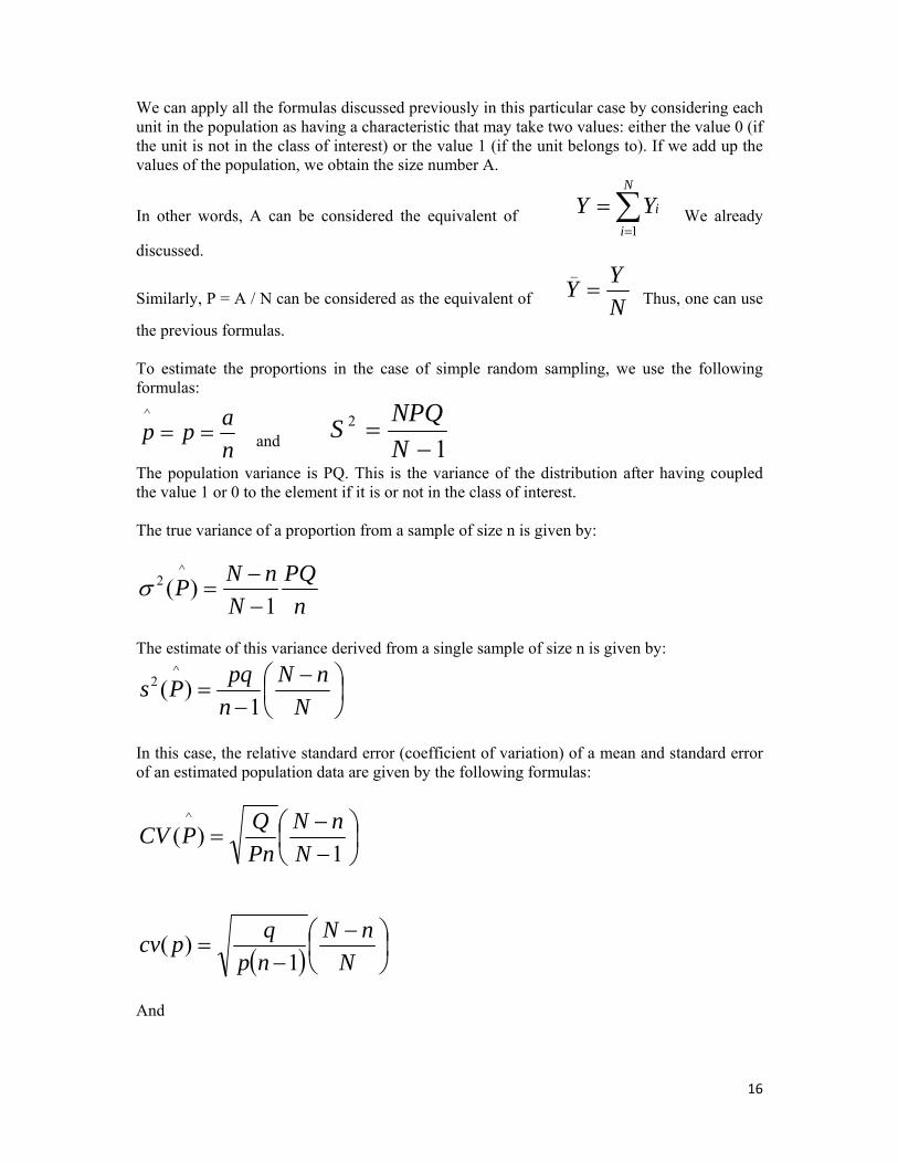
We can apply all the formulas discussed previously in this particular case by considering each unit in the population as having a characteristic that may take two values: either the value 0 (if the unit is not in the class of interest) or the value 1 (if the unit belongs to). If we add up the values of the population, we obtain the size number A.

In other words, A can be considered the equivalent of ∑=

=N

i

iYY1

We already

discussed.

Similarly, P = A / N can be considered as the equivalent of NYY =

_

Thus, one can use

the previous formulas. To estimate the proportions in the case of simple random sampling, we use the following formulas:

napp ==

^

and 12

−=

NNPQS

The population variance is PQ. This is the variance of the distribution after having coupled the value 1 or 0 to the element if it is or not in the class of interest. The true variance of a proportion from a sample of size n is given by:

nPQ

NnNP1

)(^

2

−−

=σ

The estimate of this variance derived from a single sample of size n is given by:

⎟⎠⎞

⎜⎝⎛ −

−=

NnN

npqPs

1)(

^2

In this case, the relative standard error (coefficient of variation) of a mean and standard error of an estimated population data are given by the following formulas:

⎟⎠⎞

⎜⎝⎛

−−

=1

)(^

NnN

PnQPCV

( ) ⎟⎠⎞

⎜⎝⎛ −

−=

NnN

npqpcv

1)(

And

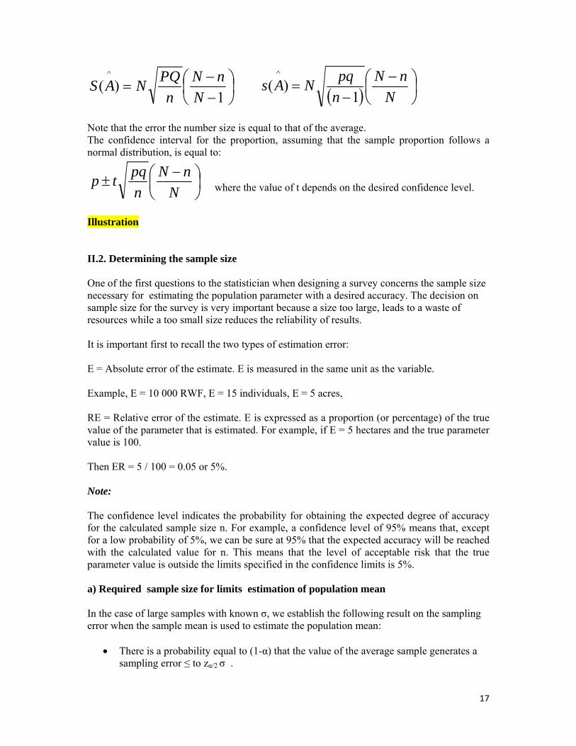
17

⎟⎠⎞

⎜⎝⎛

−−

=1

)(^

NnN

nPQNAS ( ) ⎟

⎠⎞

⎜⎝⎛ −

−=

NnN

npqNAs

1)(

^

Note that the error the number size is equal to that of the average. The confidence interval for the proportion, assuming that the sample proportion follows a normal distribution, is equal to:

⎟⎠⎞

⎜⎝⎛ −

±N

nNnpqtp where the value of t depends on the desired confidence level.

Illustration II.2. Determining the sample size One of the first questions to the statistician when designing a survey concerns the sample size necessary for estimating the population parameter with a desired accuracy. The decision on sample size for the survey is very important because a size too large, leads to a waste of resources while a too small size reduces the reliability of results. It is important first to recall the two types of estimation error: E = Absolute error of the estimate. E is measured in the same unit as the variable. Example, E = 10 000 RWF, E = 15 individuals, E = 5 acres, RE = Relative error of the estimate. E is expressed as a proportion (or percentage) of the true value of the parameter that is estimated. For example, if E = 5 hectares and the true parameter value is 100. Then ER = 5 / 100 = 0.05 or 5%. Note: The confidence level indicates the probability for obtaining the expected degree of accuracy for the calculated sample size n. For example, a confidence level of 95% means that, except for a low probability of 5%, we can be sure at 95% that the expected accuracy will be reached with the calculated value for n. This means that the level of acceptable risk that the true parameter value is outside the limits specified in the confidence limits is 5%. a) Required sample size for limits estimation of population mean In the case of large samples with known σ, we establish the following result on the sampling error when the sample mean is used to estimate the population mean:

• There is a probability equal to (1-α) that the value of the average sample generates a sampling error ≤ to zα/2 σ.

18

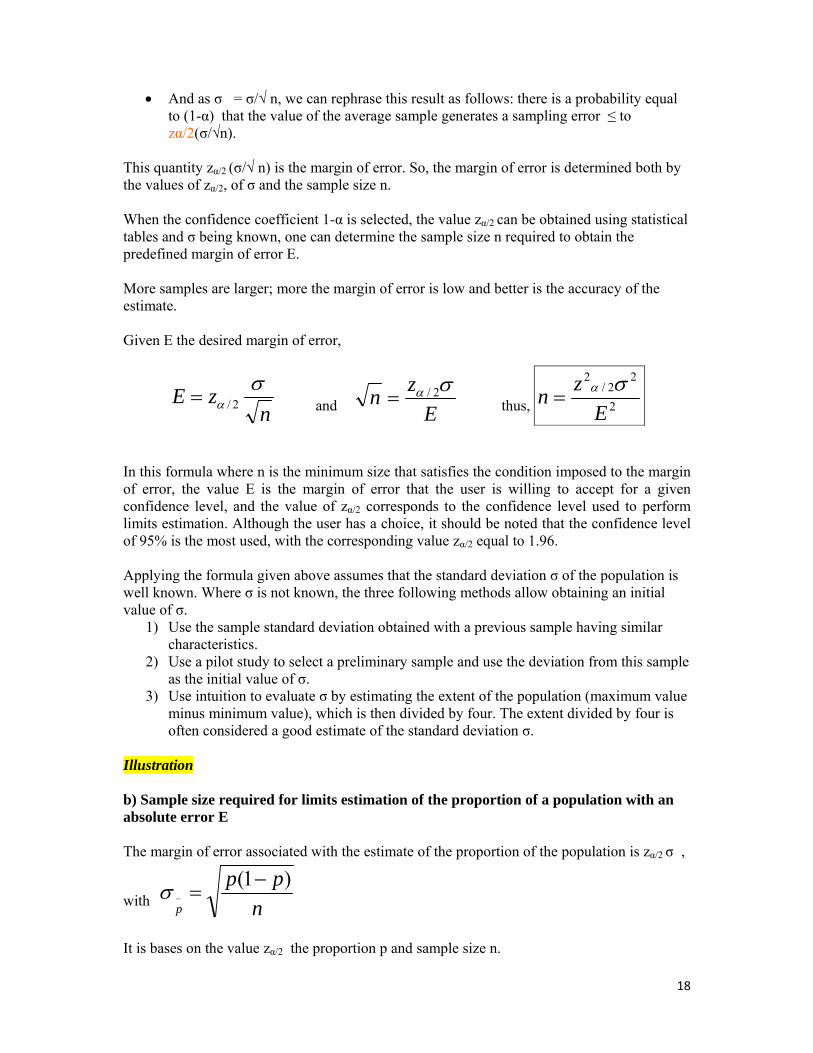
• And as σ = σ/√ n, we can rephrase this result as follows: there is a probability equal to (1-α) that the value of the average sample generates a sampling error ≤ to zα/2(σ/√n).

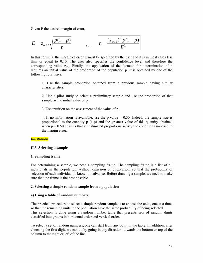
This quantity zα/2 (σ/√ n) is the margin of error. So, the margin of error is determined both by the values of zα/2, of σ and the sample size n. When the confidence coefficient 1-α is selected, the value zα/2 can be obtained using statistical tables and σ being known, one can determine the sample size n required to obtain the predefined margin of error E. More samples are larger; more the margin of error is low and better is the accuracy of the estimate. Given E the desired margin of error,

nzE σα 2/= and E

zn σα 2/= thus, 2

22/

2

Ezn σα=

In this formula where n is the minimum size that satisfies the condition imposed to the margin of error, the value E is the margin of error that the user is willing to accept for a given confidence level, and the value of zα/2 corresponds to the confidence level used to perform limits estimation. Although the user has a choice, it should be noted that the confidence level of 95% is the most used, with the corresponding value zα/2 equal to 1.96. Applying the formula given above assumes that the standard deviation σ of the population is well known. Where σ is not known, the three following methods allow obtaining an initial value of σ.

1) Use the sample standard deviation obtained with a previous sample having similar characteristics.

2) Use a pilot study to select a preliminary sample and use the deviation from this sample as the initial value of σ.

3) Use intuition to evaluate σ by estimating the extent of the population (maximum value minus minimum value), which is then divided by four. The extent divided by four is often considered a good estimate of the standard deviation σ.

Illustration b) Sample size required for limits estimation of the proportion of a population with an absolute error E The margin of error associated with the estimate of the proportion of the population is zα/2 σ,

with npp

p

)1( −=−σ

It is bases on the value zα/2 the proportion p and sample size n.

19

Given E the desired margin of error,

nppzE )1(

2/−

= α so, 2

22/ )1()(

Eppzn −

= α

In this formula, the margin of error E must be specified by the user and it is in most cases less than or equal to 0.10. The user also specifies the confidence level and therefore the corresponding value zα/2. Finally, the application of the formula for determination of n requires an initial value of the proportion of the population p. It is obtained by one of the following four ways:

1. Use the sample proportion obtained from a previous sample having similar characteristics. 2. Use a pilot study to select a preliminary sample and use the proportion of that sample as the initial value of p. 3. Use intuition on the assessment of the value of p. 4. If no information is available, use the p-value = 0.50. Indeed, the sample size is proportional to the quantity p (1-p) and the greatest value of this quantity obtained when p = 0.50 ensures that all estimated proportions satisfy the conditions imposed to the margin error.

Illustration II.3. Selecting a sample 1. Sampling frame For determining a sample, we need a sampling frame. The sampling frame is a list of all individuals in the population, without omission or duplication, so that the probability of selection of each individual is known in advance. Before drawing a sample, we need to make sure that the frame is the best possible. 2. Selecting a simple random sample from a population a) Using a table of random numbers The practical procedure to select a simple random sample is to choose the units, one at a time, so that the remaining units in the population have the same probability of being selected. This selection is done using a random number table that presents sets of random digits classified into groups in horizontal order and vertical order. To select a set of random numbers, one can start from any point in the table. In addition, after choosing the first digit, we can do by going in any direction: towards the bottom or top of the column to the right or left of the line

20

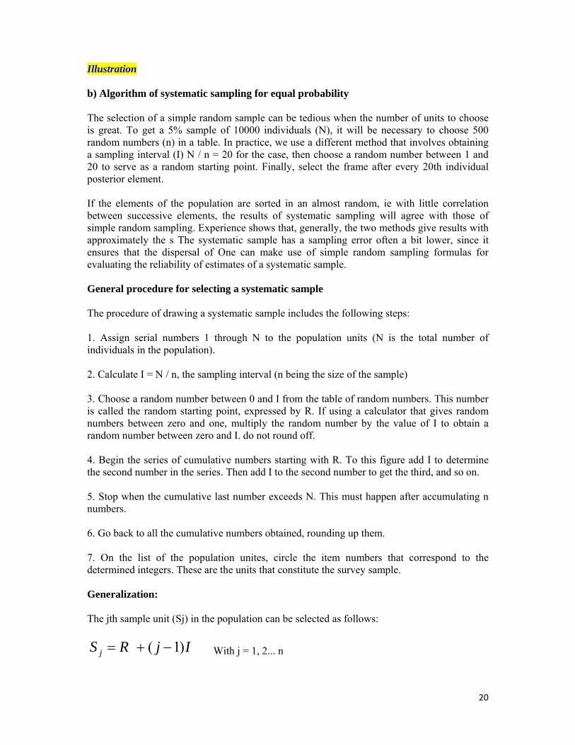
Illustration b) Algorithm of systematic sampling for equal probability The selection of a simple random sample can be tedious when the number of units to choose is great. To get a 5% sample of 10000 individuals (N), it will be necessary to choose 500 random numbers (n) in a table. In practice, we use a different method that involves obtaining a sampling interval (I) N / n = 20 for the case, then choose a random number between 1 and 20 to serve as a random starting point. Finally, select the frame after every 20th individual posterior element. If the elements of the population are sorted in an almost random, ie with little correlation between successive elements, the results of systematic sampling will agree with those of simple random sampling. Experience shows that, generally, the two methods give results with approximately the s The systematic sample has a sampling error often a bit lower, since it ensures that the dispersal of One can make use of simple random sampling formulas for evaluating the reliability of estimates of a systematic sample. General procedure for selecting a systematic sample The procedure of drawing a systematic sample includes the following steps: 1. Assign serial numbers 1 through N to the population units (N is the total number of individuals in the population). 2. Calculate I = N / n, the sampling interval (n being the size of the sample) 3. Choose a random number between 0 and I from the table of random numbers. This number is called the random starting point, expressed by R. If using a calculator that gives random numbers between zero and one, multiply the random number by the value of I to obtain a random number between zero and I. do not round off. 4. Begin the series of cumulative numbers starting with R. To this figure add I to determine the second number in the series. Then add I to the second number to get the third, and so on. 5. Stop when the cumulative last number exceeds N. This must happen after accumulating n numbers. 6. Go back to all the cumulative numbers obtained, rounding up them. 7. On the list of the population unites, circle the item numbers that correspond to the determined integers. These are the units that constitute the survey sample. Generalization: The jth sample unit (Sj) in the population can be selected as follows:

IjRS j )1( −+= With j = 1, 2... n

21

where: Sj = selected number of jth individual in the population R = random starting point; I = drawing line (interval) n = sample size

Illustration (Karongi case study)

CHAP. 3. STRATIFIED SAMPLING

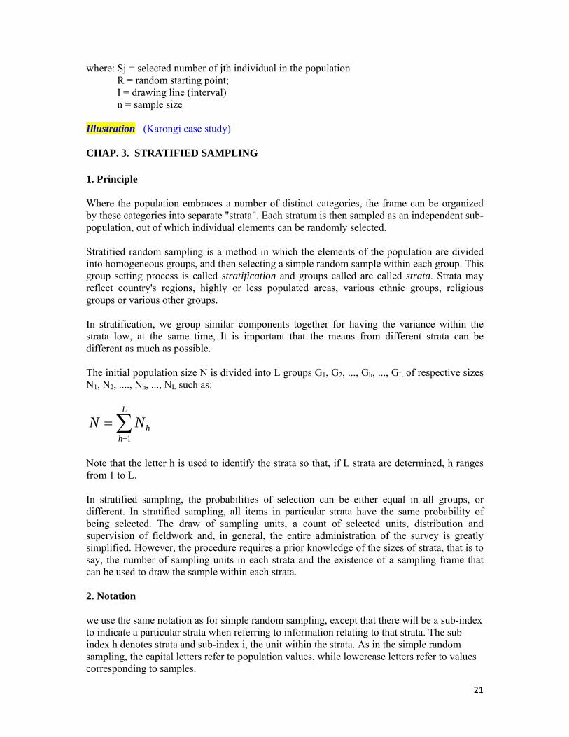
1. Principle Where the population embraces a number of distinct categories, the frame can be organized by these categories into separate "strata". Each stratum is then sampled as an independent sub-population, out of which individual elements can be randomly selected. Stratified random sampling is a method in which the elements of the population are divided into homogeneous groups, and then selecting a simple random sample within each group. This group setting process is called stratification and groups called are called strata. Strata may reflect country's regions, highly or less populated areas, various ethnic groups, religious groups or various other groups. In stratification, we group similar components together for having the variance within the strata low, at the same time, It is important that the means from different strata can be different as much as possible. The initial population size N is divided into L groups G1, G2, ..., Gh, ..., GL of respective sizes N1, N2, ...., Nh, ..., NL such as:

∑=

=L

hhNN

1

Note that the letter h is used to identify the strata so that, if L strata are determined, h ranges from 1 to L. In stratified sampling, the probabilities of selection can be either equal in all groups, or different. In stratified sampling, all items in particular strata have the same probability of being selected. The draw of sampling units, a count of selected units, distribution and supervision of fieldwork and, in general, the entire administration of the survey is greatly simplified. However, the procedure requires a prior knowledge of the sizes of strata, that is to say, the number of sampling units in each strata and the existence of a sampling frame that can be used to draw the sample within each strata. 2. Notation we use the same notation as for simple random sampling, except that there will be a sub-index to indicate a particular strata when referring to information relating to that strata. The sub index h denotes strata and sub-index i, the unit within the strata. As in the simple random sampling, the capital letters refer to population values, while lowercase letters refer to values corresponding to samples.

22

Illustration 3. Estimation

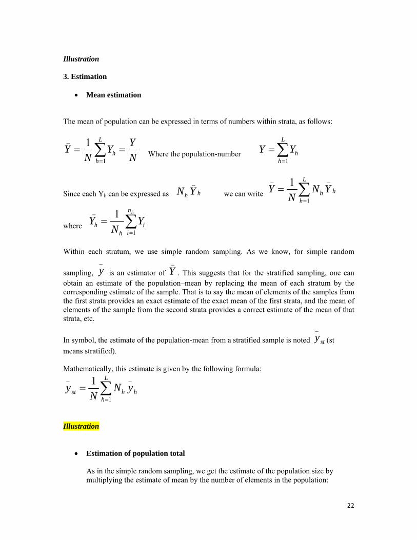
• Mean estimation The mean of population can be expressed in terms of numbers within strata, as follows:

NYY

NY

L

hh == ∑

=1

_ 1 Where the population-number ∑

=

=L

hhYY

1

Since each Yh can be expressed as hh YN_

we can write h

L

hh YN

NY

_

1

_ 1 ∑=

=

where ∑=

=hn

ii

hh Y

NY

1

_ 1

Within each stratum, we use simple random sampling. As we know, for simple random

sampling, _

y is an estimator of _

Y . This suggests that for the stratified sampling, one can obtain an estimate of the population–mean by replacing the mean of each stratum by the corresponding estimate of the sample. That is to say the mean of elements of the samples from the first strata provides an exact estimate of the exact mean of the first strata, and the mean of elements of the sample from the second strata provides a correct estimate of the mean of that strata, etc.

In symbol, the estimate of the population-mean from a stratified sample is noted sty_

(st means stratified). Mathematically, this estimate is given by the following formula:

h

L

hhst yN

Ny

_

1

_ 1 ∑=

=

Illustration

• Estimation of population total As in the simple random sampling, we get the estimate of the population size by multiplying the estimate of mean by the number of elements in the population:

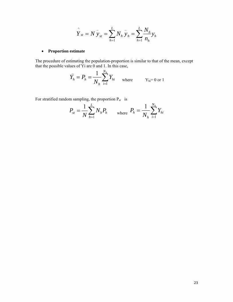
23

h

L

h h

hh

L

hhstst y

nNyNyNY ∑∑

==

===1

_

1

_^

• Proportion estimate

The procedure of estimating the population-proportion is similar to that of the mean, except that the possible values of Yi are 0 and 1. In this case,

∑=

==hN

ihi

hhh Y

NPY

1

_ 1 where Yhi= 0 or 1

For stratified random sampling, the proportion Pst is

h

L

hhst PN

NP ∑

=

=1

1 where ∑

=

=hN

ihi

hh Y

NP

1

1

24

CHAPITRE IV. SONDAGE PAR GRAPPES La présente méthode de tirage consiste à diviser d’abord la population en groupes d’éléments séparés, appelés grappes, de manière à ce que chaque élément de la population appartienne à une et une seule grappe. L’une des applications principales de l’échantillonnage par grappes est l’échantillonnage des régions géographiques, où les grappes sont notamment les quartiers d’une ville ou d’autres régions bien définies. Au Rwanda, les grappes sont notamment les Villages/Imidugudu ou les Cellules. Après ce regroupement, un échantillon aléatoire simple des grappes est ensuite sélectionné. L’échantillonnage par grappes tend à fournir de meilleurs résultats lorsque les éléments contenus dans les grappes sont hétérogènes et, dans le cas idéal, chaque grappe est une représentation à petite échelle de la population entière. La valeur de l’échantillonnage par grappes dépend du degré de représentativité de la population entière, de chaque grappe. Si toutes les grappes sont semblables dans ce sens, échantillonner un petit nombre de grappes fournira de bonnes estimations des paramètres de la population. Après la sélection des grappes échantillons, celles-ci déterminent à leur tour les unités à inclure. La détermination peut s’effectuer de deux façons suivantes : a) l’échantillon peut comprendre toutes les unités à l’intérieur des grappes choisies. Cette procédure est appelée généralement « sondage par grappes à un degré) ». b) on peut tirer un sous-échantillon des unités des grappes échantillonnées. Ceci s’appelle « sondage par grappes à plusieurs degrés » ou simplement « sondage à plusieurs degrés ». Il y a deux raisons pour l’emploi du sondage par grappes. Fréquemment, il n’existe pas de base de sondage adéquate à partir de laquelle effectuer le tirage des éléments de la population, et le coût de la construction d’une telle base de sondage serait énorme. D’autre part, une telle base pourrait exister, mais l’épargne dans les coûts des travaux de terrain obtenue avec le sondage par grappes peut faire de cette méthode une alternative plus efficace qu’un échantillon aléatoire simple. Dans la plupart de cas pratiques, un échantillon d’un effectif quelconque d’unités choisies aléatoirement aura une variance plus faible qu’un échantillon de la même taille choisi en grappes. Cependant, quand il faut balancer le coût contre la fiabilité, l’échantillon par grappes pourrait être plus efficace. Quoique les unités d’analyse ne soient pas choisies directement, la probabilité de sélection d’une grappe et de chaque unité à l’intérieur de celle-ci est connue préalablement ; ainsi donc, le sondage par grappes satisfait le critère de sondage probabiliste.

25

IV.1. Sondage aréolaire Le sondage aréolaire (area sample) est un échantillonnage à plusieurs degrés, dont l’avant dernier degré s’appuie sur des aires géographiques faisant office de grappes. Il est très utile quand une ou toutes les deux conditions suivantes existent : a) quand on ne dispose pas d’inventaires complets d’unités de logement ou autres unités d’observations, mais on dispose des cartes des entités géographiques comportant une quantité suffisante d’informations. La liste de ces cartes constitue alors une base de sondage dans la zone considérée. b) quand les frais de déplacement sont élevés, c’est-à-dire il y a un coût élevé associé aux déplacements des enquêteurs d’une unité-échantillon choisie au hasard à une autre choisie aussi au hasard. Pour le tirage d’un échantillon aréolaire, on utilisera les pâtés d’une ville comme illustration (dans les zones rurales, on peut utiliser des segments administratifs ayant des limites identifiables). On pourra procéder de la manière suivante : 1) obtenir un plan raisonnablement fidèle de la ville, qui donne le plus possible de détails sur les pâtés. Si le plan n’est pas récent, il faut prendre certaines dispositions au moyen des renseignements au niveau local pour l’actualiser ; 2) numéroter tous les pâtés successivement, en plaçant les numéros directement sur le plan, un système serpentin est conseillé pour ne pas omettre un pâté ; 3) choisir un échantillon aléatoire simple ou systématique de pâtés ; 4) interviewer tous les ménages dans les pâtés-échantillons ou sélectionner quelques ménages à l’intérieur des pâtés-échantillons, soit avec une table de nombres aléatoires, soit par sondage systématique en utilisant les numéros affectés aux unités de logement. IV.2. Estimation Il existe une analogie étroite entre le sondage par grappes et le sondage stratifié. Dans les deux cas, on regroupe les éléments individuels ensemble avant de choisir l’échantillon. La différence est que dans le sondage stratifié, il faut prélever un échantillon à l’intérieur de chaque strate, tandis que dans le sondage par grappes, on prélève un échantillon des grappes avant de choisir les éléments individuels dans les grappes-échantillons. Il convient de noter toutefois que la combinaison des deux types de sondages est souvent utilisée.

• Notation Considérons un plan de sondage à deux étapes/degrés où on choisit aléatoirement les Unités Secondaires de Sondage (USS) dans des grappes choisies (Unités Primaires de Sondage ou UPS). On a les notations suivantes : N = effectif des UPS dans la population. n = nombre de UPS choisies dans l’échantillon.

∑=

=N

iiMM

1 = effectif des unités élémentaires dans la population, et

26

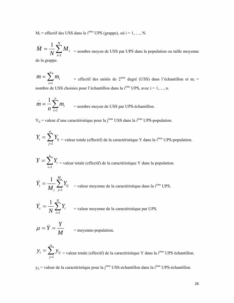
Mi = effectif des USS dans le ième UPS (grappe), où i = 1, …, N.

∑=

=N

iiM

NM

1

_ 1 = nombre moyen de USS par UPS dans la population ou taille moyenne

de la grappe.

∑=

=n

iimm

1 = effectif des unités de 2ème degré (USS) dans l’échantillon et mi =

nombre de USS choisies pour l’échantillon dans la ième UPS, avec i = 1,…, n.

∑=

=n

iim

nm

1

_ 1 = nombre moyen de USS par UPS-échantillon.

Yij = valeur d’une caractéristique pour la jème USS dans la ième UPS-population.

∑=

=iM

jiji YY

1= valeur totale (effectif) de la caractéristique Y dans la ième UPS-population.

∑=

=N

iiYY

1= valeur totale (effectif) de la caractéristique Y dans la population.

∑=

=iM

jij

ii Y

MY

1

_ 1 = valeur moyenne de la caractéristique dans la ième UPS.

∑=

=N

iic Y

NY

1

_ 1 = valeur moyenne de la caractéristique par UPS.

MYY ==

_µ = moyenne-population.

∑=

=im

jiji yy

1= valeur totale (effectif) de la caractéristique Y dans la ième UPS échantillon.

yij = valeur de la caractéristique pour la jème USS-échantillon dans la ième UPS-échantillon.

27

∑=

=im

jij

ii y

my

1

_ 1 = moyenne-échantillon de la caractéristique dans la ième UPS-

échantillon.

• Estimation des moyennes et des effectifs Les formules présentées au chapitre précédent (Stratification) pour estimer les moyennes-populations sont valables quand l’unité de sondage est identique à l’unité d’analyse. Or, une caractéristique particulière du sondage par grappes est que l’unité de sondage (au 1er degré) n’est pas l’unité d’analyse. Considérons un plan de sondage à deux étapes/degrés dans lequel les unités de la deuxième étape sont les unités d’analyse ; on choisit n grappes parmi N, par sondage aléatoire simple ; puis on choisit mi unités dans la ième UPS par sondage aléatoire simple avec i = 1, …, n. A l’intérieur de la ième grappe, la moyenne-population est donnée par :

∑=

=iM

jij

ii Y

MY

1

_ 1

Les unités à l’intérieur de la grappe étant choisies par sondage aléatoire simple, on sait qu’on peut estimer cette moyenne sans biais, à l’aide de la formule suivante :

∑=

=im

jij

ii y

my

1

_ 1

Ces estimations des moyennes au niveau de la grappe pour les n grappes-échantillons doivent être combinées pour estimer l’effectif-population global (Y) et la moyenne-population

MYY ==

_µ

Pour l’effectif-population de la caractéristique Y, on construit d’abord un estimateur non biaisé de Yi, l’effectif de la caractéristique Y dans la ième UPS, qui est donnée par :

ii

ii y

mMY =

^

Ainsi, un estimateur non biaisé pour l’effectif-population est :

∑ ∑∑∑∑= ====

====n

i

m

jij

i

ii

n

ii

n

ii

i

in

ii

i

ymM

nNyM

nNy

mM

nNY

nNY

1 1

_

111

^^

De la même façon, on peut estimer la moyenne-population ∑

∑

=

==== N

ii

N

ii

M

Y

MYY

1

1_

µ

28

Un estimateur de _Y est :

∑∑==

==im

j i

ijn

i

i

my

M

MnNy

11^

_^µ où ∑

=

=n

iiM

nNM

1

^

Il importe de noter que pour l’estimation d’une proportion, la formule est la même, sauf que l’on considère seulement les yij = 1, c’est-à-dire les unités possédant l’attribut. Illustration IV.3. Sondage à plusieurs degrés

On est par exemple dans une ville où l’on doit procéder à une enquête par grappes à plusieurs étapes/degrés. La ville est constituée de : Un quartier = UPS (Unité Primaire de Sondage) ; Un bloc = USS (Unité Secondaire de Sondage) ; Un immeuble = UTS (Unité Tertiaire de Sondage) ; Des ménages = UQS (Unité Quaternaire de Sondage). Parallèlement aux sondages à probabilités égales, il existe des plans de sondage où les individus ont des probabilités d’inclusion inégales. Généralement, les tirages stratifiés et les tirages à plusieurs degrés sont des tirages où les individus de la base de sondage n’ont pas tous la même probabilité d’être sélectionnés. Une sélection avec probabilité proportionnelle à la taille signifie, par exemple, qu’une grappe qui est 5 fois plus grande qu’une autre aura 5 fois de probabilité de tomber dans l’échantillon.

Comme résultat du tirage à plusieurs degrés, la possibilité que n’importe quelle unité de la dernière étape soit comprise dans l’échantillon est le produit des probabilités de sélection de toutes les toutes les étapes effectuées.

L’illustration du sondage à plusieurs degrés nous amènera au tirage systématique déjà évoqué, mais avec des probabilités égales. Pour le cas présent, l’algorithme du tirage systématique est appliqué avec des probabilités inégales.

Calcul des probabilités et facteurs d’extrapolation

1. Probabilité de tirage d’une UPS (grappe), au 1er degré

h

hihh M

MaP =1

avec Mh = nombre de ménages dans la strate h

ah = nombre d’UPS (grappes) tirées dans la strate h

29

Mhi = nombre de ménages dans l’UPS (grappe) i de la strate h

2. Probabilité de tirage d’un ménage, au 2ème degré

hi

hijh M

mP =2

avec mhij = nombre de ménages tirés dans l’UPS (grappe) i de la strate h

3. Probabilité globale de tirage d’un ménage dans la strate h

hhh PPP 21 .=

4. Facteur d’extrapolation dans une strate

hhhh PPPW 21 ./1/1 ==

5. Probabilité de tirage d’un ménage dans toutes les strates (niveau national, par exemple)

∏=h

hPP

6. Facteur d’extrapolation dans toutes les strates (niveau national, par exemple)

∏==h

hPPW /1/1

EXERCICE : Cas de l’enquête de Karongi

30

CHAPTER VI. SAMPLING IN TIME (Panel) Taking into account the time will add a dimension to the issue of the survey. The difference between the values of a variable Y on the individuals of a given population is likely to be not only spatial but also temporal. Indeed, the time will intervene in the definition of two fundamental concepts: population and variables. No one can deny that populations evolve over time, as the variables are affected by time. If we look at a complex parameter ∆ that compares two similar parameters, but set at two different times t and t +1. If both parameters are noted θt and θt+1 (∆ can be the difference θt+1- θt or the ratio θt+1/θt). One question will be raised about the reference population at time t Ωt or involve both population Ωt (where we define θ t) and population Ωt +1 (where we θ t +1) This duality of approaches will impact on the choice of sampling method, but it may also reconcile the two by opting for a rotating sample plan. If we study a population Ωt defined at time t and we measure the changes over time in this population, we are in presence of a longitudinal survey. In another case, when the study intends to describe the status of a population at one point, we talk about a cross-sectional survey. Whether the approach is longitudinal or transverse, we can use three types of surveys: samples drawn independently at each date, panels and rotating samples. However, we often use panels or rotating samples. VI.1. Panels in longitudinal approach When attempting to measure the evolution of a parameter over time, the population being that of the original date, it often happens that one chooses to take a sample from the original date, and follow the individuals in the sample as long as it is relevant for the purposes of the study. Such a sample when individuals are interviewed at least twice is called a panel. Panels can be used because the parameter we want to estimate explicitly involves the individual developments of the variable of interest. Example, for calculation of monthly price indexes, it is necessary to establish a range of products to estimate the index. The establishment of a panel can be done to minimize errors of observation which necessarily affect the results of surveys. IV.2. Panels in transverse approach Using a panel seems inconsistent with the estimation of a parameter to the current date. Indeed, a panel is a sample that represents the population set to its drawing. To move from an initial population (old) to the current one (contemporary),we need to take into account the new individuals. To move from the panel to the transverse sample, we must ensure that each individual of the current population can be sampled. The principle is to avoid probabilities of zero selection. For this, there are three methods:

31

• Making a stratum (or strata) gathering new individuals, defined as individuals who belong to the current population without being in the initial population. Then, we draw from this stratum to form the necessary complement. This method has the major drawback of being based on the knowledge of all new individuals. • Either you draw, regardless of the panel, a sample in the cross-sectional population. Thus, each individual will have a new non-zero probability of inclusion in the final sample. • Either we use a combination "natural" individuals and we decide to investigate the entire group if and only if it contains at least one individual of the panel. This methodology known as "indirect sampling" is not infallible, but significantly reduces the problem. For example, to conduct a physical survey of individuals, as individuals are grouped into units or households, they may decide to investigate the current date all the people who are in housing or households that contain at least one individual panel. IV.3. Ratational Sampling a) Principle The rotary rotational sampling consists of taking regular (quarterly or annual) samples panelized for a given period, common to all panels. Thus, at each survey date (called a "wave"), a panel enters the system while a panel comes out. The main advantages of the rotary sampling are those of the panel, namely the gain of accuracy in estimating the changes and the reduction of the observation error. However, this sampling has some drawbacks; including difficulties in monitoring field where a change of panel address of individuals (this is sometimes called "tracing" or "tracking" of individuals). b) Longitudinal exploitation In times of change between dates t and t +1, assume that each panel must be interviewed four times, eg every quarter for one year. The sample taken at the time α will be investigated to waves α, α +1, α+ 2 and α +3. c) Transverse exploitation In this approach, it is estimated, for example, the total Tt where t is the current date. At each date t, we practice an inference on the entire population Ωt. Regarding the protocol for the collection, we follow all the individuals of the panel in time and we question all individuals living in the same housing or household as the sample person.