Introduction — Analysis of Reservoir Performan ce Slide — 1(20 November 2002)

(Formation Evaluation and the Analys is of Reservoir Performance)

Modu le for:Analysis of Reservoir Performance

Introduction

T.A. Blasingame, Texas A&M U.Department of Petroleum Engineering

Texas A&M UniversityCollege Station, TX 77843-3116

(979) 845-2292 — t-blasingame@tamu.edu

Introduction — Analysis of Reservoir Performan ce Slide — 2(20 November 2002)

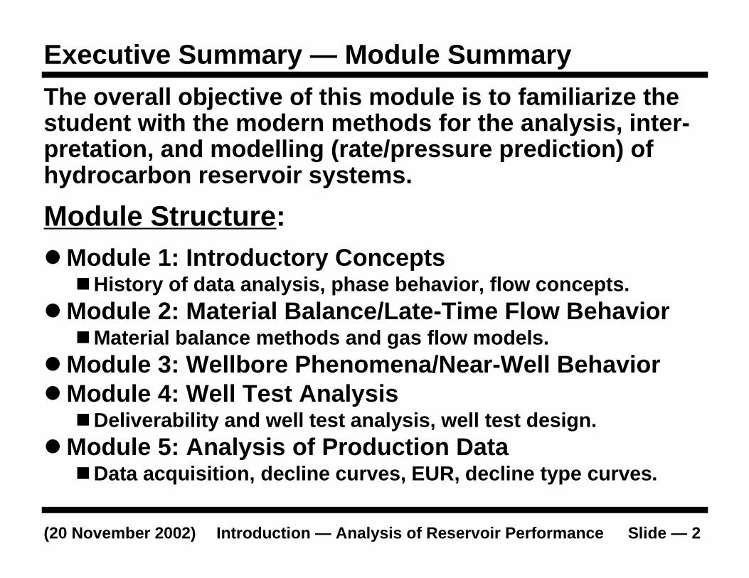
Executive Summary — Module Summary

�Module 1: Introdu ctory Concepts�History of data analys is , phase behavior, flow concepts.

�Module 2: Material Balance/Late-Time Flow Behavior�Material balance methods and gas flow models.

�Module 3: Wellbore Phenomena/Near-Well Behavior�Module 4: Well Test Analys is

�Deliverabili ty and well test analysis, well test design.�Module 5: Analys is of Produ ction Data

�Data acquis it ion, decline curves, EUR, decline type curves.

The overall ob jective of this modu le is to famili arize thestudent with the modern method s for the analys is , inter-pretation, and modelling (rate/pressure prediction) ofhydrocarbon reservoir systems.

Modu le Structure:

Introduction — Analysis of Reservoir Performan ce Slide — 3(20 November 2002)

Executive Summary — Modu le Objectives

�Course Objectives: (the student shoul d be able to ...)� Derive the steady-state and pse udosteady-state flow equations for horizontal linear and

radial flow of liquids and gases (including the pseudopressure and pressure-squaredformulations). Sketch pressure versus time and pressure versus distance t rends for areservoir sys tem exhibiting transient, pseudosteady-state, and steady-state flow behavior.

� Derive the "skin factor" variable from the steady-state flow equation and be able to descr ibethe conditions of damage and stimulation u sing this variable.

� Define and use dimensionless va riables and dimensionless solutions to il lustrate the genericperformance of a particular reservoir model.

� Derive the analys is and interpretation methodologies (i.e., "conventional plots" and typecurve analysis) for pressu re drawdown and pressure buildup tests , for liquid, gas, andmultiphase flow sys tems. This effo rt should incl ude t he use of pseudopressure andpseudotime concepts for the analys is of well test and pr oduction data from dry gas andsolution-gas drive oil reservoir systems).

� Apply dimensionless solutions (" type curves" ) and field var iable solutions ("specializedplots" ) for the foll owing "well test" cases: unfractured and fractured wells in i nfin ite andfinite-acting, homogeneous and d ual porosity reservoirs.

� Design and implement a well test sequence, as well as a long-term production/injectionsurveillance program.

� Analyze production data (rate-time or pressure-rate-time data) to o btain reservoir volumeand estimates of reservoir properties for gas and liquid reservoir syst ems. Also b e able topredict production performance using simplified solutions.

� Demonstrate the capabil ity to integrate, analyze, and interpret well test and production datato characterize a reservoir in terms of reservoir pr operties and performance potential (f ieldstudy project).

Introduction — Analysis of Reservoir Performan ce Slide — 4(20 November 2002)

�History of Data Analysis�Correlation p lots — cumulative-IP, rate-time, etc.�Rate-time correlations (log-log, semilog, etc.).�Arps rate-time relations (expon ential/hyperbolic).

�Phase Behavior�Gas z-factor (Standing-Katz correlation plot(s)).�Gas compressibili ty.�Gas visco sity.

�Fund amentals of Fluid Flow in Porous Media�General form of the gas diffusiv ity equation .�Pseudop ressure-pseudo time form.�Pressure-squared form.�Pseudotime and pressure-squared criteria plots.

Modu le 1: Introdu ctory Concepts

Introduction — Analysis of Reservoir Performan ce Slide — 5(20 November 2002)

Modu le 1: History of Data Analysis — Data Plots

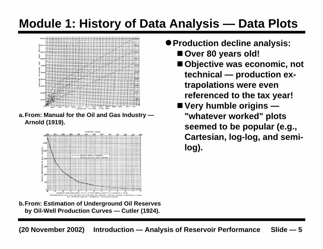
�Production decline analysi s:�Over 80 years old!�Objective was economic, not

technical — production ex-trapolations were evenreferenced to the tax year!

�Very humble origins —"whatever worked" plotsseemed to be pop ular (e.g.,Cartesian, log-log, and semi-log).

a.From: Manual for the Oil and Gas Industry —Arnold (1919).

b.From: Estimation of Undergroun d Oil Reservesby Oil-Well Production Curves — Cutler (1924).

Introduction — Analysis of Reservoir Performan ce Slide — 6(20 November 2002)

Modu le 1: History of Data Analysis — Rate Plots

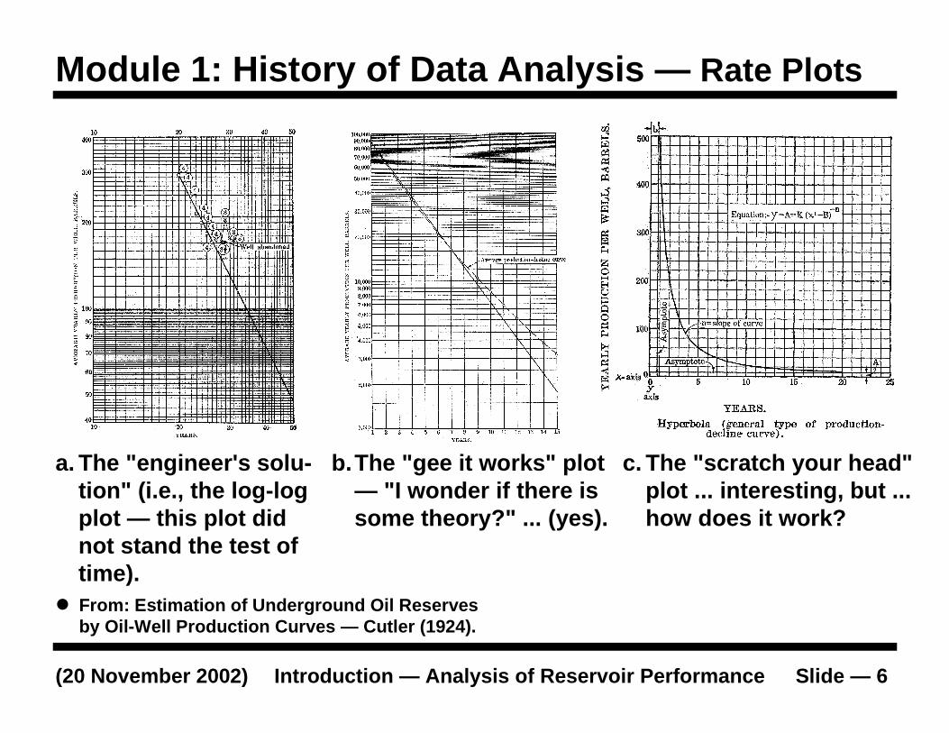
� From: Estimation of Underground Oil Reservesby Oil-Well Production Curves — Cutler (1924).

a. The "engineer's solu-tion" (i.e., the log-logplot — this plot didnot stand the test oftime).

b.The "gee it works" plot— " I wonder if there issome theory?" ... (yes).

c. The "scratch your head"plot ... interesting, but ...how does it work?

Introduction — Analysis of Reservoir Performan ce Slide — 7(20 November 2002)

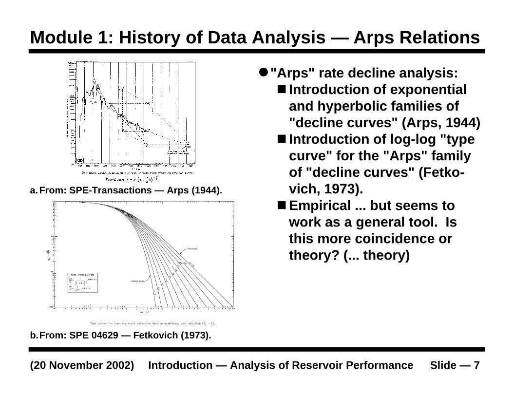
Modu le 1: History of Data Analysis — Arps Relations

�"Arps" rate decline analys is:� Introdu ction o f expon ential

and hyperbolic famili es of"decline curves" (Arps, 1944)

� Introdu ction o f log-log " typecurve" for the "Arps" familyof "decline curves" (Fetko-vich, 1973).

�Empirical ... but seems towork as a general tool. Isthis more coincidence ortheory? (... theory)

a.From: SPE-Transactions — Arps (1944) .

b.From: SPE 04629 — Fetkovich (1973).

Introduction — Analysis of Reservoir Performan ce Slide — 8(20 November 2002)

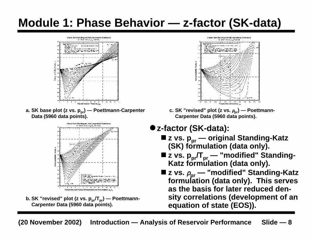
Modu le 1: Phase Behavior — z-factor (SK-data)

a. SK base plot (z vs. ppr) — Poettmann-CarpenterData (5960 data points).

b. SK " revised" plot (z vs. ppr/Tpr) — Poettmann-Carpenter Data (5960 data points).

�z-factor (SK-data):� z vs . ppr — original Standing-Katz

(SK) formulation (data only).� z vs . ppr/Tpr — "modified" Standi ng-

Katz formulation (data only).� z vs . ρρρρpr — "modified" Standing-Katz

formulation (data only). This servesas the basis for later reduced den-sity correlations (development of anequation of state (EOS)).

c. SK " revised" plot (z vs. ρρρρpr) — Poettmann-Carpenter Data (5960 data points).

Introduction — Analysis of Reservoir Performan ce Slide — 9(20 November 2002)

Modu le 1: Phase Behavior — z-factor (DAK-EOS)

a. SK base plot (z vs. ppr) — Original Dranchuk-Abou-Kassem data fit (DAK-EOS).

b. SK " revised" plot (z vs. ppr/Tpr) — OriginalDranchuk-Abou-Kassem data fit (DAK-EOS).

�z-factor (DAK-EOS):� z vs . ppr — Original Dranchuk-Abou-

Kassem data fit (DAK-EOS).� z vs . ppr/Tpr — "modified" Standi ng-

Katz formulation, original Dranchuk-Abou-Kassem data fit (DAK-EOS).

� z vs . ρρρρpr — "modified" Standing-Katzformulation, original Dranchuk-Abou-Kassem data fit (DAK-EOS).

c. SK " revised" plot (z vs. ρρρρpr) — Original Dranchuk-Abou-Kassem data fit (DAK-EOS).

Introduction — Analysis of Reservoir Performan ce Slide — 10(20 November 2002)

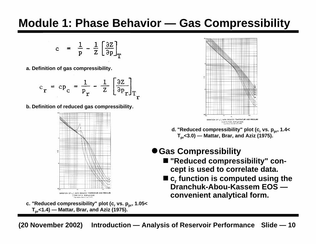
Module 1: Phase Behavior — Gas Compress ibility

a. Definition of gas compressib ili ty .

c. "Reduced compressibili ty" plot (cr vs . ppr, 1.05<Tpr<1.4) — Mattar, Brar, and Aziz (1975).

�Gas Compressibility� "Reduced compress ibil ity" con-

cept is used to correlate data.� cr function is computed using the

Dranchuk-Abou-Kassem EOS —convenient analytical form.

d. "Reduced compressibili ty" plot (cr vs . ppr, 1.4<Tpr<3.0) — Mattar, Brar, and Aziz (1975).

b. Definition of reduced gas compressib ili ty .

Introduction — Analysis of Reservoir Performan ce Slide — 11(20 November 2002)

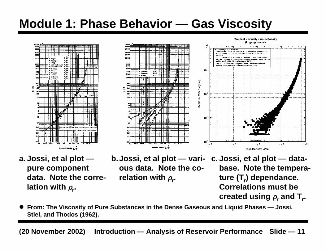
Modu le 1: Phase Behavior — Gas Viscosity

� From: The Viscosity of Pure Substances in the Dense Gaseous and Liquid Phases — Joss i,Stiel, and Thodos (1962).

a. Joss i, et al plot —pure componentdata. Note th e corre-lation wi th ρρρρr.

b.Joss i, et al plot — vari-ous data. Note the co-relation wi th ρρρρr.

c. Joss i, et al plot — data-base. Note the tempera -ture (Tr) dependance.Correlations must becreated using ρρρρr and Tr.

Introduction — Analysis of Reservoir Performan ce Slide — 12(20 November 2002)

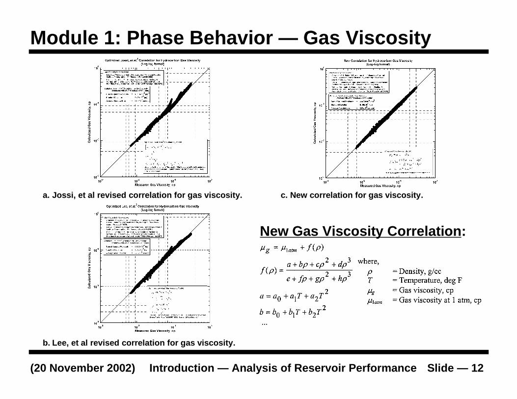
Modu le 1: Phase Behavior — Gas Viscosity

a. Jossi, et al revised correlation for gas viscosity.

b. Lee, et al revised correlation for gas viscosity.

c. New correlation for gas visco sity.

New Gas Viscosity Correlation :

Introduction — Analysis of Reservoir Performan ce Slide — 13(20 November 2002)

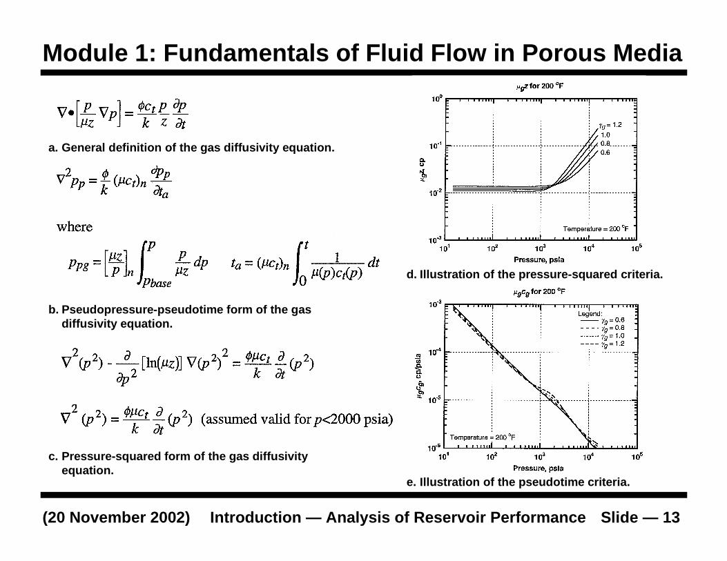
Module 1: Fundamentals of Fluid Flow i n Porous Media

a. General definition of the gas diffusivity equation.

c. Pressure-squared form of the gas diffusivityequation.

b. Pseudopressure-pseudotime form of the gasdiffusivity equation.

d. Illustration of the pressure-squared criteria.

e. Illustration of the pseudotime criteria.

Introduction — Analysis of Reservoir Performan ce Slide — 14(20 November 2002)

�Gas Material Balance�Dry gas reservoir sys tems.�Water drive gas reservoir sys tems.�"Abno rmally-pressured" gas reservoir systems.�Generalized gas material balance equation .

�Late-Time Flow Behavior�Simplified flow behavior (empirical relations).�Exponential decline (liquid flow solution).�Simplified (approximate) gas flow relation.

Modu le 2: Material Balance

Introduction — Analysis of Reservoir Performan ce Slide — 15(20 November 2002)

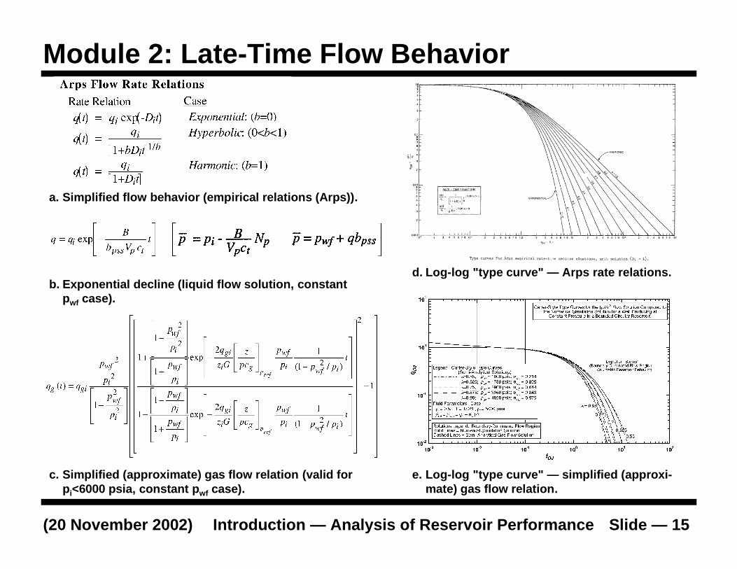
Modu le 2: Late-Time Flow Behavior

a. Simpli fied flow behavior (empirical relations (Arps)).

c. Simpli fied (approximate) gas flow relation (valid forpi<6000 psia, constant pwf case).

b. Exponential decline (liquid flow solution, constantpwf case).

d. Log-log " type curve" — Arps rate relations .

e. Log-log " type curve" — simpli fied (approxi-mate) gas flow relation .

Introduction — Analysis of Reservoir Performan ce Slide — 16(20 November 2002)

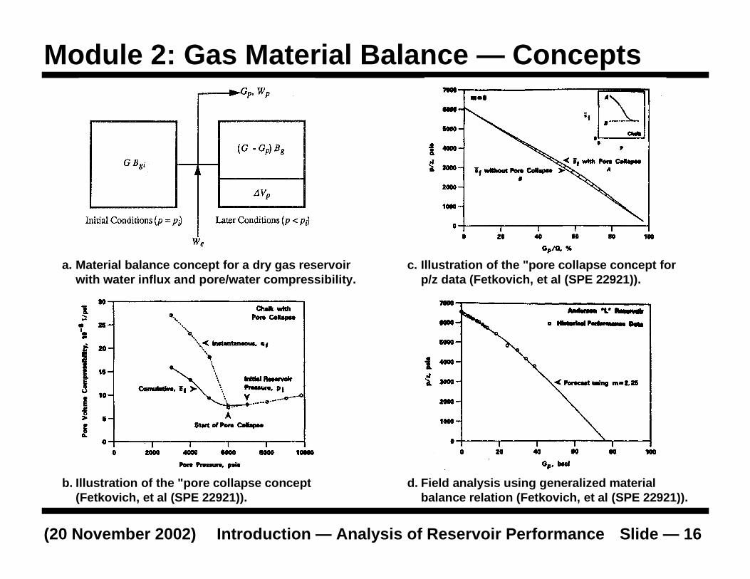
Modu le 2: Gas Material Balance — Concepts

a. Material balance concept for a dry gas reservoirwith water influx and p ore/water compress ib ili ty.

b. Illustration of the "pore collapse concept(Fetkovich, et al (SPE 22921)).

d. Field analysis using generalized materialbalance relation (Fetkovich, et al (SPE 22921)).

c. Illustration of the "pore collapse concept forp/z data (Fetkovich, et al (SPE 22921)).

Introduction — Analysis of Reservoir Performan ce Slide — 17(20 November 2002)

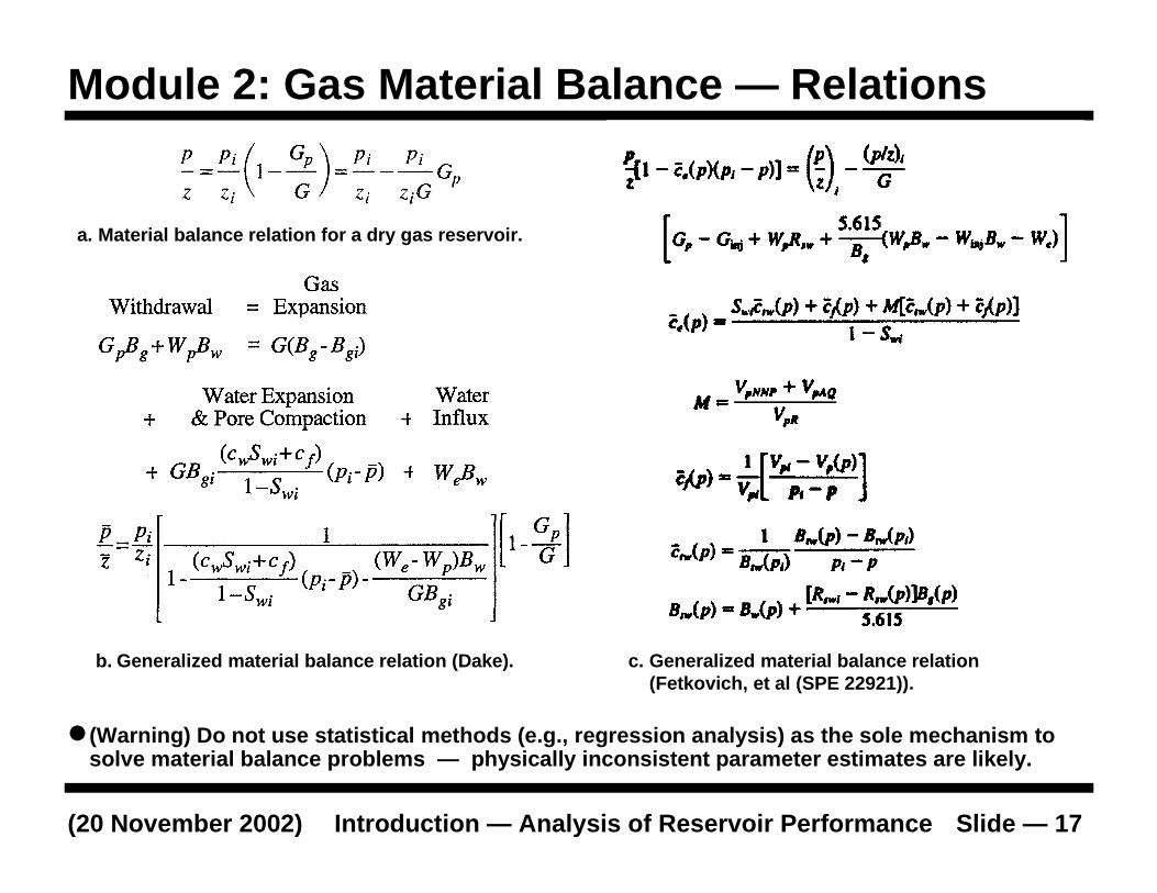
Modu le 2: Gas Material Balance — Relations

a. Material balance relation for a dry gas reservoir.

b. Generalized material balance relation (Dake). c. Generalized material balance relation(Fetkovich, et al (SPE 22921)).

�(Warning) Do not use statistica l methods (e.g., regression analysis) as the sole mechanism tosolve material balance problems — physically inconsistent parameter estimates are likely.

Introduction — Analysis of Reservoir Performan ce Slide — 18(20 November 2002)

�Calculation of Bott omhole Pressures�General relation (energy balance)�Static (non -flowing) bottomhole pressure (dry gas).�Flowing bo ttomhole pressure (dry gas).

�Near-Well Reservoir Flow Behavior�Steady-state "skin factor" concept used to represent

damage or stimulation in the near-well region.�"Variable" sk in effects: non -Darcy flow, well cleanup ,

and g as cond ensate banking.

Modu le 3: Wellbore Phenomena/Near-Well Behavior

Introduction — Analysis of Reservoir Performan ce Slide — 19(20 November 2002)

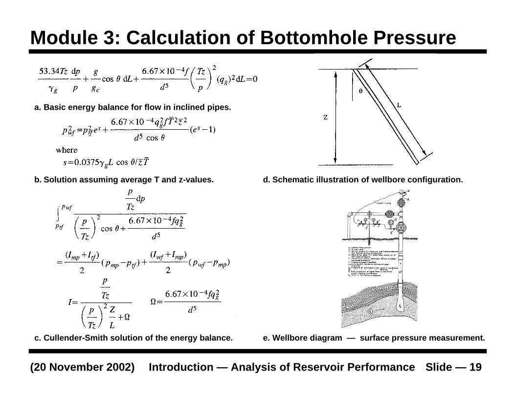
Modu le 3: Calculation of Bott omhole Pressure

a. Basic energy balance for flow in inclined pipes.

d. Schematic illustration of wellbore configuration.b. Solution assuming average T and z-values.

e. Wellbore diagram — surface pressure measurement.c. Cullender-Smith solution of the energy balance.

Introduction — Analysis of Reservoir Performan ce Slide — 20(20 November 2002)

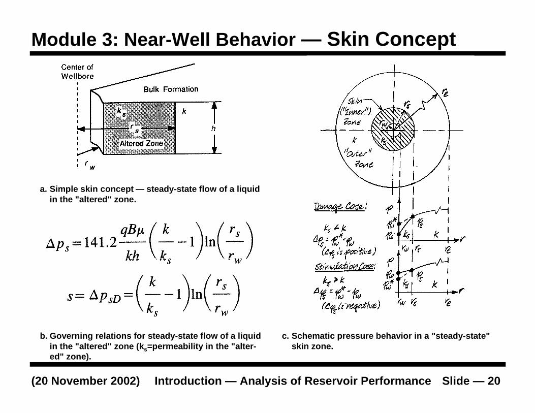
Modu le 3: Near-Well Behavior — Skin Concept

a. Simple sk in concept — steady-state flow of a liquidin the "altered" zone.

c. Schematic pressure behavior in a "steady-state"sk in zone.

b. Governing relations for steady-state flow of a liquidin the "altered" zone (ks=permeabili ty in the "alter-ed" zone).

Introduction — Analysis of Reservoir Performan ce Slide — 21(20 November 2002)

Modu le 3: Extensions of the Skin Concept

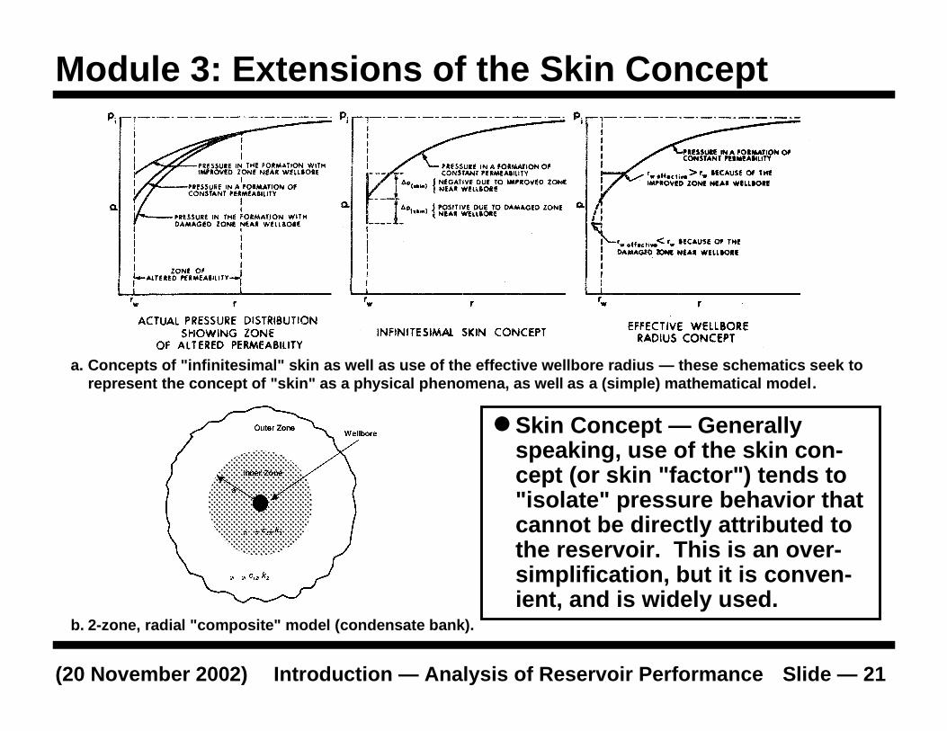
a. Concepts of " infinitesimal" skin as well as use of the effective wellbore radius — these sch ematics seek torepresent the concept o f "sk in" as a physical phenomena, as well as a (simple) mathematical model .

b. 2-zone, radial "composite" model (condensate bank).

�Skin Concept — Generallyspeaking, use of the skin con-cept (or sk in " factor" ) tends to" isolate" pressure behavior thatcannot be directly att ributed tothe reservoir. This is an over-simplification, but it is conven-ient, and is widely used.

Introduction — Analysis of Reservoir Performan ce Slide — 22(20 November 2002)

� Orientation — This modu le wil l focus speci-fically on the analysis and i nterpretation ofdeliverabili ty test data and pressu re transienttest data. The issues must be clear: test de-sign, data acquisit ion/ data quali ty cont rol, andtest execution are crit ical activ it ies .

� Deliverabili ty Testing:� Keep it simple — a "4-point" test is appropriate.� Isochronal testing is very diff icult to implement.

� Pressure Transient Test Analys is/Interpretation:� Conventional analysis is consistent/approp riate.� Model identification (log-log (or type curve) analysis).� Test design — keep it simple.

Modu le 4: Well Test Analys is

Introduction — Analysis of Reservoir Performan ce Slide — 23(20 November 2002)

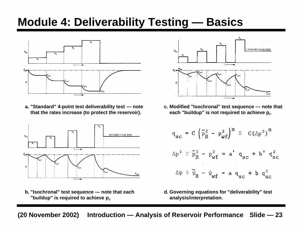
Modu le 4: Deliverabil ity Testing — Basics

a. "Standard" 4-point test deliverabili ty test — notethat the rates increase (to protect the reservoir).

b. " Isochronal" test sequence — note that each"buildup" is required to achieve p i.

c. Modified " Isochronal" test sequence — note thateach "buildup" is not required to achieve p i.

d. Governing equations for "deliverabili ty" testanalys is/interpretation.

Introduction — Analysis of Reservoir Performan ce Slide — 24(20 November 2002)

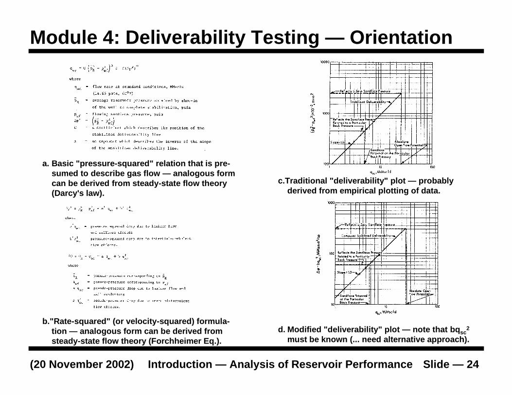
Modu le 4: Deliverabil ity Testing — Orientation

a. Basic "pressure-squared" relation that is pre-sumed to describe gas flow — analogous formcan be derived from steady-state flow theory(Darcy 's law).

b."Rate-squared" (or velocity-squared) formula-tion — analogous form can be derived fromsteady-state flow theory (Forchheimer Eq.).

d. Modified "deliverabili ty" plot — note that bqsc2

must be known (... need alternative approach).

c.Traditional "deliverabili ty" plot — probablyderived from empirical plotting of data.

Introduction — Analysis of Reservoir Performan ce Slide — 25(20 November 2002)

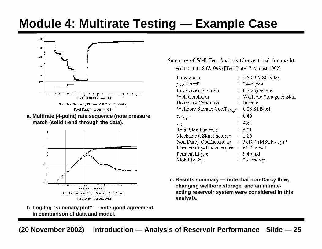
Modu le 4: Multirate Testing — Example Case

a. Multirate (4-point) rate sequence (note pressurematch (solid trend through the data).

b. Log-log "summary plot" — note good agreementin comparison of data and model.

c. Results summary — note that non-Darcy flow,changing wellbore storage, and an infin ite-acting reservoir sys tem were considered in thisanalys is.

Introduction — Analysis of Reservoir Performan ce Slide — 26(20 November 2002)

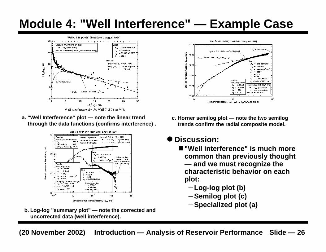
Modu le 4: "Well Interference" — Example Case

a. "Well Interference" plot — note the linear trendthrough the data functions (confirms interference) .

b. Log-log "summary plot" — note the corrected anduncorrected data (well i nterference).

c. Horner semilog plot — note the two semilogtrends confirm the radial composite model.

�Discuss ion:�"Well i nterference" is much more

common than previously thought— and we must recognize thecharacteristic behavior on eachplot:–Log-log plot (b)–Semilog plot (c)–Specialized plot (a)

Introduction — Analysis of Reservoir Performan ce Slide — 27(20 November 2002)

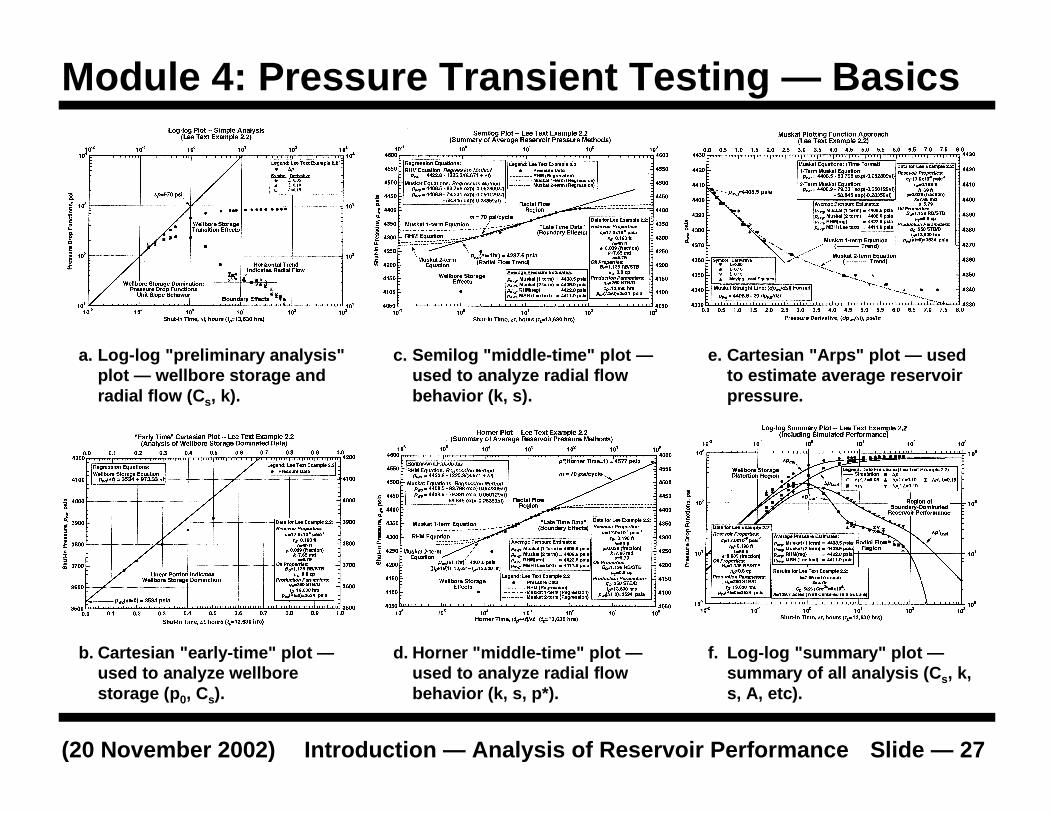
Modu le 4: Pressure Transient Testing — Basics

a. Log-log "preliminary analysis"plot — wellbore storage andradial flow (Cs, k).

b. Cartesian "early-time" plot —used to analyze wellborestorage (p0, Cs).

c. Semilog "middle-time" plot —used to analyze radial flowbehavior (k, s).

d. Horner "middle-time" plot —used to analyze radial flowbehavior (k, s, p*).

f. Log-log "summary" plot —summary of all analysis (Cs, k,s, A, etc).

e. Cartesian "Arps" plot — usedto estimate average reservoirpressure.

Introduction — Analysis of Reservoir Performan ce Slide — 28(20 November 2002)

� Produ ction data — " low frequen cy" (taken atlarge (or even rando m) intervals) and " lowresolution" (data quali ty (i.e., accuracy) isminimal).

� Simple Analysis:� Rate-time decline curve analys is .� EUR analysis (usually rate-cumulative or variation).� New stuff — advanced analys is based on a simple,

yet robust model (e.g., Knowles qg-Gp analysis)� Decline type curve analys is:

� Systematic, model-based analysis approach.� Model identification — transient data analys is .� Volume estimates — pseudosteady-stat e behavior is

dictated by material balance (very consistent).

Modu le 5: Analys is of Production Data

Introduction — Analysis of Reservoir Performan ce Slide — 29(20 November 2002)

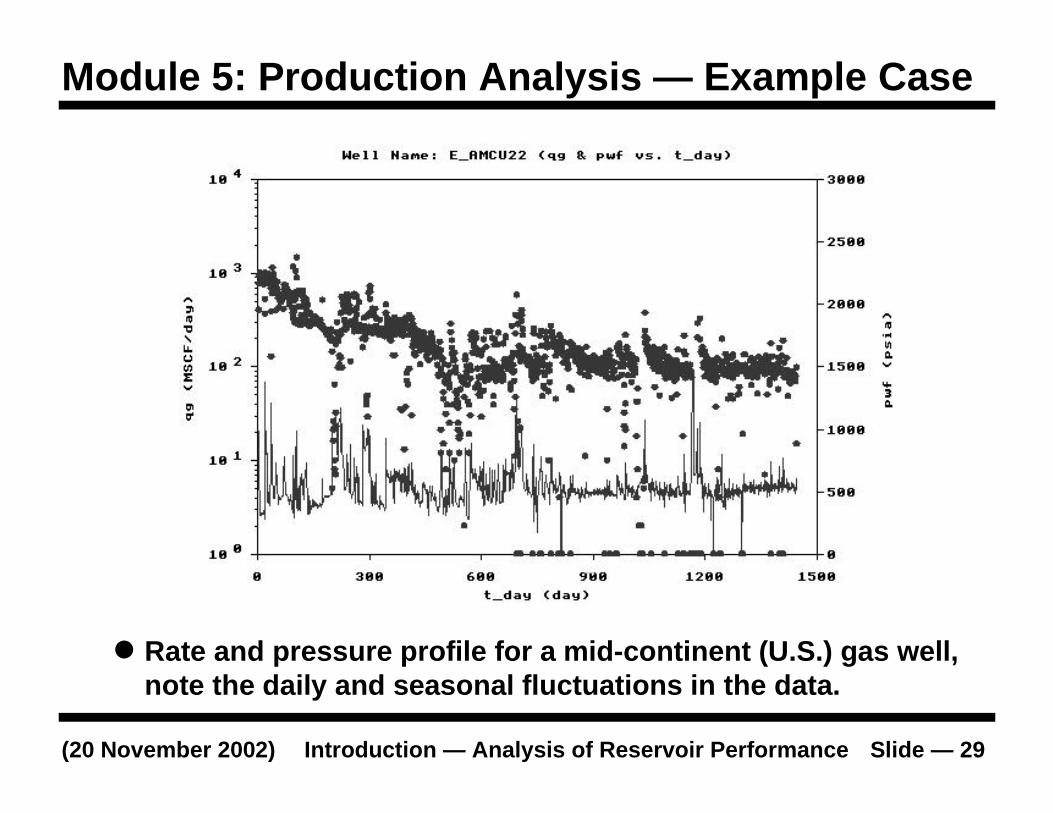
Modu le 5: Produ ction Analys is — Example Case

� Rate and pressure profile for a mid-continent (U.S.) gas well,note the daily and seasonal f luctuations in the data.

Introduction — Analysis of Reservoir Performan ce Slide — 30(20 November 2002)

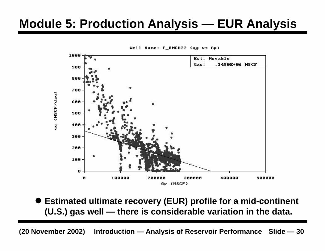
Modu le 5: Produ ction Analys is — EUR Analysis

� Estimated ultimate recovery (EUR) profile for a mid-continent(U.S.) gas well — there is considerable variation in the data.

Introduction — Analysis of Reservoir Performan ce Slide — 31(20 November 2002)

Module 5: Production Analys is — WPA Approac h

� Note that the WPA approach provides a un ique analysi s/interpretation of the well performance history.

Introduction — Analysis of Reservoir Performan ce Slide — 32(20 November 2002)

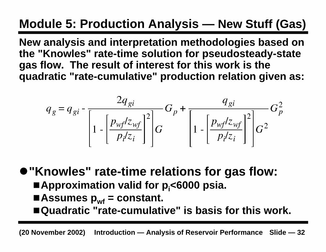
Modu le 5: Produ ction Analys is — New Stuff (Gas)

�"Knowles" rate-time relations for gas flow:�Approximation valid for pi<6000 psia.�Assumes pwf = constant.�Quadratic " rate-cumulative" is basis for this work.

New analys is and interpretation methodo logies based onthe "Knowles" rate-time solution for pseudo steady-stategas flow. The result of interest for this work is thequadratic " rate-cumulative" produ ction relation given as:

Introduction — Analysis of Reservoir Performan ce Slide — 33(20 November 2002)

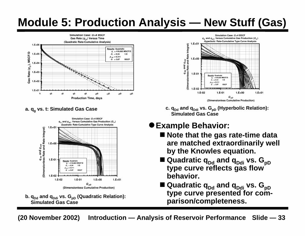
a. qg vs. t: Simulated Gas Case

b. qDd and qDdi vs . GpD (Quadratic Relation):Simulated Gas Case

�Example Behavior:� Note that the gas rate-time data

are matched extraordinarily wellby the Knowles equation.

� Quadratic qDd and qDdi vs . GpDtype curve reflects gas flowbehavior.

� Quadratic qDd and qDdi vs . GpDtype curve presented for com-parison/completeness.

c. qDd and qDdi vs . GpD (Hyperbolic Relation):Simulated Gas Case

Modu le 5: Produ ction Analys is — New Stuff (Gas)

Introduction — Analysis of Reservoir Performan ce Slide — 34(20 November 2002)

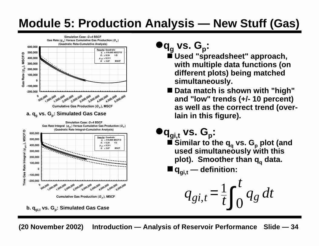
a. qg vs. Gp: Simulated Gas Case

b. qgi,t vs. Gp: Simulated Gas Case

�qgi,t vs. Gp:� Similar to the qq vs . Gp plot (and

used simultaneously with thisplot). Smoother than qq data.

�qgi,t — definition:

�qg vs . Gp:� Used "spreadsheet" approach,

with multiple data functions (ondifferent plots) being matchedsimultaneously.

� Data match is shown with " high"and " low" trends (+/- 10 percent)as well as the correct trend (over-lain in this figure).

dtqt

tq gtgi

0 1

, ∫=

Modu le 5: Produ ction Analys is — New Stuff (Gas)

Introduction — Analysis of Reservoir Performan ce Slide — 35(20 November 2002)

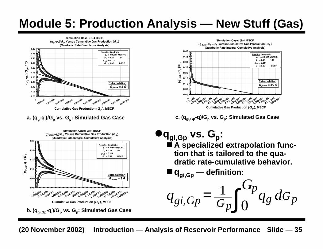
a. (qg-qi)/Gp vs. Gp: Simulated Gas Case

b. (qgi,Gp-qi)/Gp vs . Gp: Simulated Gas Case

�qgi,Gp vs. Gp:� A specialized extrapolation func-

tion that is tailored to the qua-dratic rate-cumulative behavior.

�qgi,Gp — definition:

pGgp

pGGpgi dqG

q

0

1, ∫=

c. (qgi,Gp-q)/Gp vs . Gp: Simulated Gas Case

Modu le 5: Produ ction Analys is — New Stuff (Gas)

Introduction — Analysis of Reservoir Performan ce Slide — 36(20 November 2002)

Modu le 5: Produ ction Analys is — the hard way...

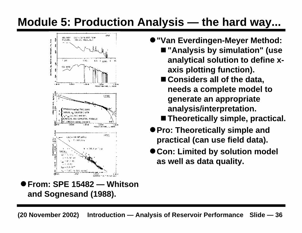
�From: SPE 15482 — Whitsonand Sognesand (1988).

�"Van Everdingen-Meyer Method:� "Analysis by simulation" (use

analytical solution to define x-axis plott ing function).

�Considers all of the data,needs a complete model t ogenerate an appropriateanalys is/interpretation .

�Theoretically simple, practical.�Pro: Theoretically simple and

practical (can use field data).�Con: Limited by solution model

as well as data quali ty.

Introduction — Analysis of Reservoir Performan ce Slide — 37(20 November 2002)

Modu le 5: Produ ction Analys is — History Lessons

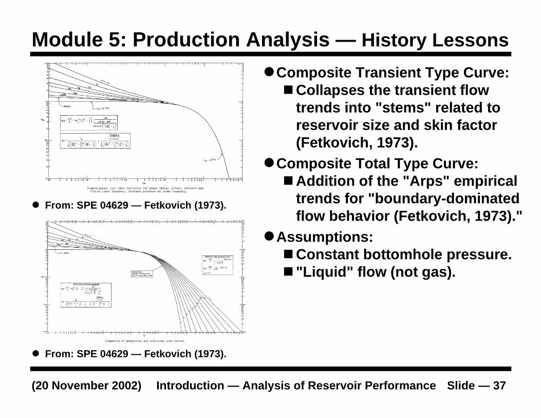
� From: SPE 04629 — Fetkovich (1973).

� From: SPE 04629 — Fetkovich (1973).

�Composite Transient Type Curve:�Collapses the transient flow

trends into "stems" related toreservoir size and sk in factor(Fetkovich, 1973).

�Composite Total Type Curve:�Addition of the "Arps" empirical

trends for "bou ndary-dominatedflow behavior (Fetkovich, 1973)."

�Assumptions:�Constant bottomhole pressure.� "Liqu id" flow (not gas).

Introduction — Analysis of Reservoir Performan ce Slide — 38(20 November 2002)

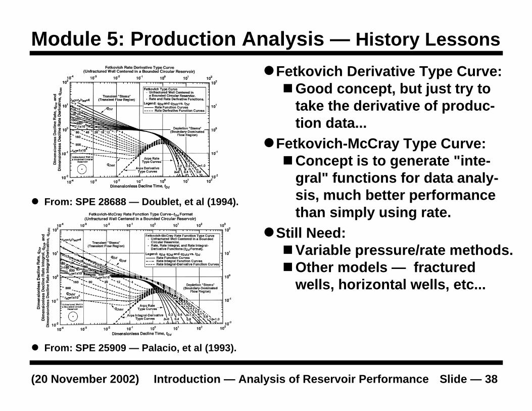
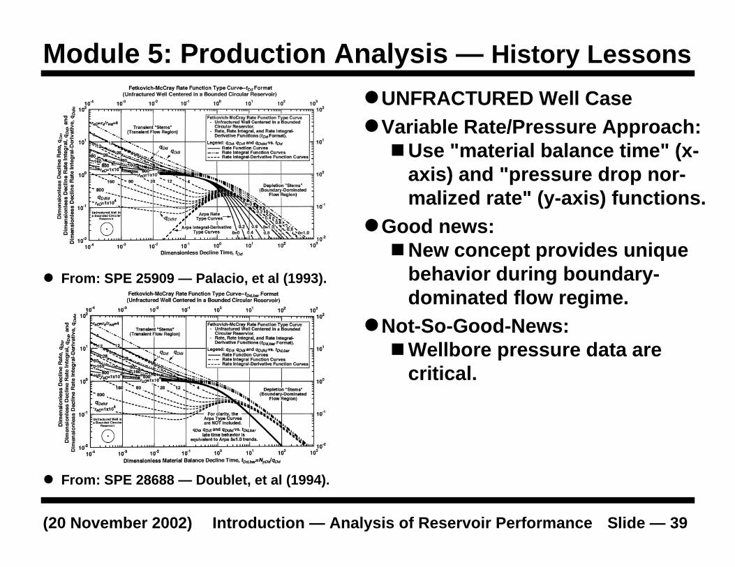
� From: SPE 25909 — Palacio, et al (1993).

� From: SPE 28688 — Doublet, et al (1994).

�Fetkovich Derivative Type Curve:�Good concept, but just try to

take the derivative of produ c-tion data...

�Fetkovich-McCray Type Curve:�Concept is to generate " inte-

gral" functions for data analy-sis, much better performancethan simply using rate.

�Still Need:�Variable pressure/rate methods.�Other models — fractured

wells, horizontal wells , etc...

Modu le 5: Produ ction Analys is — History Lessons

Introduction — Analysis of Reservoir Performan ce Slide — 39(20 November 2002)

� From: SPE 25909 — Palacio, et al (1993).

� From: SPE 28688 — Doublet, et al (1994).

�UNFRACTURED Well Case�Variable Rate/Pressure Approach:

�Use "material balance time" (x-axis) and "pressure drop nor-malized rate" (y-axis) functions.

�Good news:�New concept provides unique

behavior during bound ary-dominated flow regime.

�Not-So-Good -News:�Wellbore pressure data are

critical.

Modu le 5: Produ ction Analys is — History Lessons

Introduction — Analysis of Reservoir Performan ce Slide — 40(20 November 2002)

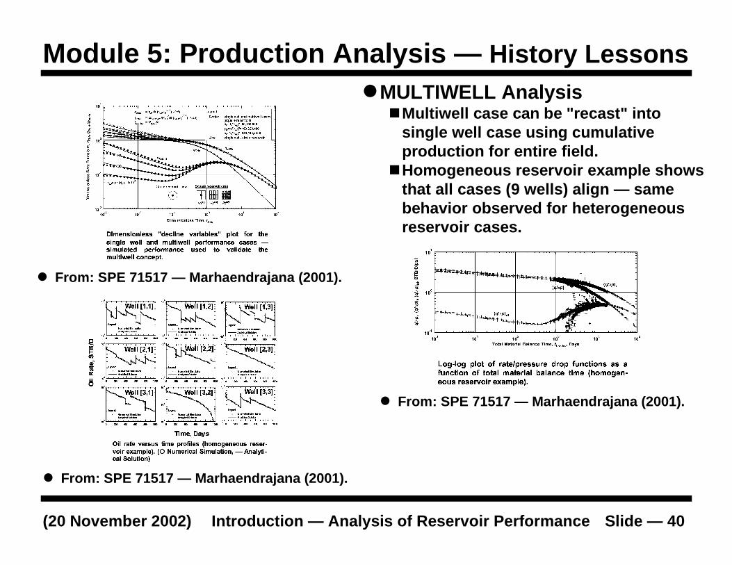
� From: SPE 71517 — Marhaendrajana (2001).

� From: SPE 71517 — Marhaendrajana (2001).

�MULTIWELL Analysis�Multiwell case can be " recast" into

single well case using cumulativeproduction for entire field.

�Homogeneous reservoir example showsthat all cases (9 wells) align — samebehavior observed for heterogeneousreservoir cases.

� From: SPE 71517 — Marhaendrajana (2001).

Modu le 5: Produ ction Analys is — History Lessons

Introduction — Analysis of Reservoir Performan ce Slide — 41(20 November 2002)

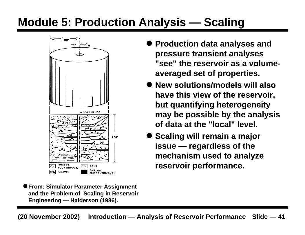
�From: Simulator Parameter Ass ignmentand the Problem of Scaling in ReservoirEngineering — Halderson (1986).

� Production data analyses andpressure transient analyses"see" the reservoir as a volume-averaged set of properties.

� New solutions/models will alsohave this view of t he reservoir ,but quantifying heterogeneitymay be poss ible by the analys isof data at the " local" level.

� Scaling will remain a majorissue — regardless of themechanism used to analyzereservoir performance.

Modu le 5: Produ ction Analys is — Scaling

Introduction — Analysis of Reservoir Performan ce Slide — 42(20 November 2002)

� Future of Produ ction Data Analys is:�Evolutionary changes:

– Better data acquisition (major issue).– Multiwell analys is (major issue).– Better software (major issue).– More reservoir/well solutions (minor issue).

�Revolutionary changes:– Direct dataflow into integrated packages for

analys is/simulation (5-10 years).– Real-time rate-pressure optimization, simul-

taneous monitoring and control (5-10 years).

Modu le 5: Produ ction Analys is — Future

Introduction — Analysis of Reservoir Performan ce Slide — 43(20 November 2002)

(Formation Evaluation and the Analys is of Reservoir Performance)

Modu le for:Analysis of Reservoir Performance

Introduction

T.A. Blasingame, Texas A&M U.Department of Petroleum Engineering

Texas A&M UniversityCollege Station, TX 77843-3116

(979) 845-2292 — t-blasingame@tamu.edu

End of Presentation